Fixed-Point Properties of the Bellman Operator in Discounted Stochastic Maintenance Optimization

Abstract

This paper investigates an infinite-horizon discounted stochastic maintenance optimization problem within the framework of dynamic programming. The system degradation is modeled by a discrete-time stochastic process affected by maintenance actions and random disturbances, while the objective is to minimize the expected discounted maintenance and degradation costs. The analysis is carried out on the Banach space of continuous functions equipped with the supremum norm. It is proved that the associated Bellman operator is well defined, maps the function space into itself, and is a contraction with contraction modulus equal to the discount factor. Consequently, the existence and uniqueness of the optimal value function follow from the Banach Fixed Point Theorem, and the convergence of value iteration is established. In addition, rigorous a priori and a posteriori error estimates are derived, providing theoretical stopping criteria for numerical computation. The theoretical results are complemented by numerical experiments illustrating the optimal stationary maintenance policy, the stability of the computed solution under grid refinement, and the influence of the discount factor on both the optimal policy and the convergence rate of value iteration.

1. Introduction

Maintenance optimization is an important problem in reliability engineering, operations research, and industrial asset management [1]. Maintenance decisions affect both current operating costs and the future condition of a system, and an effective maintenance policy must therefore balance the cost of intervention against the consequences of continued deterioration. Over the past several decades, maintenance planning has developed from predominantly corrective strategies toward systematic approaches based on reliability models, condition information, and optimization methods [2,3,4,5].

Uncertainty in the deterioration process is an important part of many maintenance problems. Over time, a system may be affected by operating conditions, environmental effects, and random disturbances, and in that case, maintenance decisions must follow the system condition changes. Stochastic dynamic programming gives a natural framework for these problems because it accounts for both the immediate cost of a maintenance action and its effect on future system behavior [6,7,8,9,10].

For discounted infinite-horizon problems, the optimal expected cost is characterized by the Bellman equation. The Bellman operator is central to the analysis because its properties determine whether the optimality equation has a unique solution and whether value iteration converges to that solution. In particular, if the Bellman operator is well defined on a complete function space and is a contraction, the Banach Fixed Point Theorem guarantees the existence and uniqueness of the fixed point, together with the convergence of successive approximations [8,9,11].

The literature on maintenance optimization is extensive. Classical surveys provide comprehensive overviews of maintenance models and their applications [4], while more recent reviews summarize developments in condition-based maintenance, stochastic deterioration models, and multi-component systems [5]. Recent studies continue to investigate stochastic maintenance optimization using Markov decision processes and dynamic programming in a variety of maintenance settings [12,13,14]. Maintenance theory and reliability-based decision problems are treated systematically in standard monographs [2,3], whereas the mathematical foundations of sequential stochastic decision problems are well established in the literature on dynamic programming and Markov decision processes [6,7,8,9].

Although these studies consider a variety of maintenance settings and optimization strategies, the present paper focuses on the mathematical properties of the Bellman operator associated with a discounted stochastic maintenance model. Rather than proposing a new maintenance strategy, the aim is to provide a rigorous fixed-point analysis of the model, establish the well-posedness and contraction properties of the Bellman operator, derive convergence and error estimates for value iteration, and illustrate these theoretical results through numerical experiments.

The model describes a system whose degradation state belongs to a compact interval. Maintenance actions are selected from a compact admissible set, and the state dynamics combine natural degradation growth, the effect of maintenance, and a bounded random disturbance. The objective is to minimize the expected discounted sum of maintenance and degradation-related costs over an infinite planning horizon.

The analysis is carried out on the Banach space of continuous real-valued functions on the compact state space, equipped with the supremum norm [15,16]. Under the assumptions imposed on the model, the Bellman operator is shown to map this space into itself and to be a contraction with modulus equal to the discount factor. These properties imply the existence and uniqueness of the optimal value function and the uniform convergence of value iteration. The contraction argument also yields a priori and a posteriori error estimates that can be used to assess the convergence of successive approximations [17,18,19]. The minimizing actions in the Bellman equation are then used to characterize the optimal stationary maintenance policy.

The theoretical results are complemented by a numerical study. Value iteration is implemented on finite state and action grids, and linear interpolation is used when the next state does not coincide with a grid point. The numerical experiments illustrate the optimal maintenance policy, examine the stability of the computed solution under grid refinement, and investigate the effect of the discount factor on the optimal policy and the convergence rate of value iteration. The observed convergence behavior is also compared with the contraction factors predicted by the theoretical analysis.

The contribution of the paper is therefore the complete analysis of the proposed stochastic maintenance model within a consistent theoretical and computational framework. The model assumptions are connected explicitly to the properties of the Bellman operator; the contraction argument is used to establish existence, uniqueness, convergence, and error estimates; and the resulting optimal maintenance problem is studied numerically. The numerical experiments provide additional insight into the structure of the optimal policy and illustrate the relationship between the theoretical contraction factor and the observed convergence behavior of value iteration.

The remainder of the paper is organized as follows. Section 2 introduces the fixed-point and functional-analytic concepts used in the analysis. Section 3 formulates the stochastic maintenance problem and defines the associated Bellman operator. Section 4 establishes the main theoretical results concerning the Bellman operator, the optimal value function, value iteration, error estimates, and the optimal stationary maintenance policy. Section 5 presents the numerical analysis, including the baseline solution, grid refinement, the influence of the discount factor, and convergence diagnostics. The final section summarizes the main conclusions and outlines possible directions for further work.

2. Preliminaries

This section provides the mathematical concepts that will be used in the paper. We focus only on the functional analysis necessary for the formulation of the stochastic maintenance optimization problem and the subsequent analysis of the associated Bellman operator.

2.1. Function Spaces

Let $(X,d)$ be a metric space. The space of all bounded and continuous real-valued functions defined on X is denoted by

$$C_b\left(X\right)=\left\{V:X\to \mathbb{R}:V\mathrm{is}\mathrm{bounded}\mathrm{and}\mathrm{continuous}\right\}.$$

The space $C_b\left(X\right)$ is endowed with the supremum norm

$${\parallel V\parallel }_{\infty }=\underset{x\in X}{sup}\left|V\left(x\right)\right|.$$

Equipped with this norm, $C_b\left(X\right)$ is a Banach space [15,16]. Note that, since X is compact, $C_b\left(X\right)$ coincides with the space of continuous functions $C\left(X\right)$.

In our paper, the value function will be observed in the space $C_b\left(X\right)$, which will provide the functional setting for the analysis of the Bellman operator associated with the discounted stochastic maintenance optimization problem.

2.2. Contraction Mappings and Banach Fixed Point Theorem

The notion of a contraction mapping plays a fundamental role in the analysis developed in this paper.

Definition 1.

Let $(Y,\parallel ·\parallel )$ be a Banach space. A mapping

$$T:Y\to Y$$

is called a contraction if there exists a constant $\beta \in (0,1)$ such that

$$\parallel Tv-Tw\parallel \le \beta \parallel v-w\parallel ,v,w\in Y.$$

The following classical result provides the theoretical foundation for the existence, uniqueness, and approximation of the value function.

Theorem 1

(Banach Fixed Point Theorem [20]). Let $(Y,\parallel ·\parallel )$ be a Banach space, and let

$$T:Y\to Y$$

be a contraction with contraction constant $\beta \in (0,1)$.

Then the following assertions hold:

1.

There exists a unique fixed point $v^{*}\in Y$ such that

$$T{v}^{*}=v^{*}.$$

2.

For every initial approximation $v_0\in Y$, the sequence defined recursively by

$$v_{n+1}=T{v}_n,n=0,1,2,\dots ,$$

converges to the unique fixed point $v^{*}$.

The Banach Fixed Point Theorem also provides quantitative estimates for the distance between the approximate solution $v_n$ and the unique fixed point $v^{*}$.

The a priori error estimate is given by

$$\parallel v_n-v^{*}\parallel \le {\displaystyle \frac{{\beta }^n}{1-\beta }}\parallel v_1-v_0\parallel ,n=0,1,2,\dots .$$

(1)

This estimate provides an upper bound for the approximation error in terms of the initial difference $\parallel v_1-v_0\parallel$ and the contraction constant $\beta$. To achieve a prescribed accuracy $\epsilon$, the required number of iterations satisfies

$$n\ge {\displaystyle \frac{ln\left({\displaystyle \frac{\epsilon (1-\beta )}{\parallel v_1-v_0\parallel }}\right)}{ln\left(\beta \right)}}.$$

(2)

The a posteriori error estimate is given by

$$\parallel v_n-v^{*}\parallel \le {\displaystyle \frac{\beta }{1-\beta }}\parallel v_n-v_{n-1}\parallel ,n=1,2,\dots .$$

(3)

This estimate allows termination of the numerical algorithm without knowing the exact solution. Unlike the a priori estimate, the a posteriori estimate depends only on two successive iterates and is therefore particularly useful for constructing rigorous stopping criteria in numerical implementations.

Finally, the geometric convergence estimate is

$$\parallel v_n-v^{*}\parallel \le {\beta }^n\parallel v_0-v^{*}\parallel ,n=0,1,2,\dots .$$

(4)

Thus, the sequence of successive approximations converges geometrically to the unique fixed point, with convergence rate determined by the contraction constant $\beta$. A smaller value of the parameter $\beta$ results in a stronger contraction of the operator and a smaller number of iterations.

While the Banach Fixed Point Theorem provides the theoretical foundation adopted in this paper, fixed-point theory has been substantially extended through the development of iterative algorithms for solving variational inequalities, equilibrium problems, and convex optimization problems. Recent studies have proposed efficient fixed-point iterations and parallel algorithms with strong convergence properties in real Hilbert spaces and demonstrated their applicability to systems of variational inequalities [21,22,23]. Although the present paper relies on the classical Banach contraction principle rather than on developing a new iterative scheme, these contributions highlight the broad applicability of fixed-point methods and further justify the mathematical framework employed in the analysis of the Bellman operator.

2.3. Discounted Cost Minimization and the Bellman Operator

We consider a discrete-time infinite-horizon discounted optimization problem. At each decision period, the system occupies a state $x\in X$, and an admissible action u is selected in order to minimize the expected total discounted cost.

For a value function $v\in C_b\left(X\right)$, the Bellman operator is introduced in the general form [6,11]

$$\left(Tv\right)\left(x\right)=\underset{u\in U\left(x\right)}{min}\left\{c(x,u)+\beta \mathbb{E}\left[v\left(x^{\prime }\right)\right]\right\},$$

(5)

where $x\in X$ is the current state, $U\left(x\right)$ is the set of admissible actions available at state x, $u\in U\left(x\right)$ is the selected action, $c(x,u)$ is the one-period cost associated with state x and action u, $\beta \in (0,1)$ is the discount factor, $x^{\prime }$ denotes the next state of the system, and $\mathbb{E}$ denotes expectation with respect to the random disturbance governing the state transition.

The specific form of the state space, the admissible action set, the running cost, and the stochastic transition equation used in this paper will be introduced in Section 3.

The Bellman operator transforms a candidate value function into a new function obtained by minimizing the sum of the current cost and the expected discounted continuation value.

The analytical results required for the subsequent application of the Banach Fixed Point Theorem consist of proving that the Bellman operator maps the chosen Banach space into itself and that it satisfies a contraction property. These properties will be established for the specific stochastic maintenance optimization model in Section 4.

3. Problem Formulation: Cost Function, Dynamics and Bellman Operator

In the context of infinite-horizon maintenance cost minimization, we consider the Bellman operator T introduced in (5) on the Banach space $C_b\left(X\right)$ equipped with the standard supremum norm ${\parallel ·\parallel }_{\infty }$.

The state space is defined by

$$X=[0,M],$$

where $x\in X$ denotes the current degradation state of the system, and $M>0$ denotes the maximum admissible degradation level.

The admissible action space is defined by

$$U=[0,u_{max}],$$

where $u\in U$ denotes the maintenance action, or maintenance intensity, and $u_{max}>0$ denotes the maximum admissible maintenance intensity. Since U is a closed and bounded interval of $\mathbb{R}$, it is compact.

For an arbitrary value function $v\in C_b\left(X\right)$, the Bellman operator is defined by

$$\left(Tv\right)\left(x\right)=\underset{u\in U}{min}\left\{A{u}^2+B{x}^2+Cx+\beta \mathbb{E}\left[v\left(x^{\prime }\right)\right]\right\},x\in X,u\in U.$$

(6)

The instantaneous maintenance cost is defined by

$$c(x,u)=A{u}^2+B{x}^2+Cx,$$

(7)

where $A,B,C>0$ are model parameters.

The coefficient A represents the weight assigned to the direct cost of maintenance effort. The quadratic term $A{u}^2$ penalizes large maintenance actions and reflects the increasing cost associated with higher maintenance intensity.

The coefficient B represents the weight assigned to the quadratic degradation cost. The term $B{x}^2$ penalizes high degradation levels more strongly as the degradation state increases.

The coefficient C represents the weight assigned to the linear degradation-related cost. The term $Cx$ accounts for the immediate cost associated with the current degradation level.

The assumptions $A,B,C>0$ ensure that all components of the instantaneous cost are nonnegative for $x\ge 0$ and $u\ge 0$. In particular,

$${\displaystyle \frac{{\partial }^{2}c}{\partial u^2}}(x,u)=2A>0,$$

so the instantaneous cost function is strictly convex with respect to the maintenance action u. Moreover,

$${\displaystyle \frac{\partial c}{\partial x}}(x,u)=2Bx+C>0$$

for every $x\ge 0$, which means that the degradation-related cost is strictly increasing with the degradation state.

The stochastic state transition equation is defined by

$$x^{\prime }=min\left\{(1-\eta u)x+d+\epsilon ,M\right\},$$

(8)

where

• $x^{\prime }$ denotes the degradation state in the next decision period;
• $\eta \in (0,1)$ is the maintenance efficiency parameter;
• $d>0$ denotes the deterministic degradation increment during one decision period;
• $\beta \in (0,1)$ is the discount factor (which also represents the contraction constant);
• $\epsilon$ is a real-valued random disturbance satisfying

  $$\mathbb{E}\left[\epsilon \right]=0$$

  and

  $$\epsilon \ge -d\mathrm{almost}\mathrm{surely}.$$

The condition $\epsilon \ge -d$ almost surely ensures that the random disturbance cannot offset more than the deterministic degradation increment d.

For the maintenance model to remain meaningful, the coefficient multiplying the current degradation state x, namely $1-\eta u$, must remain positive for every admissible maintenance action. Therefore, we impose

$$u_{max}<{\displaystyle \frac{1}{\eta }}.$$

(9)

Since $u\in U=[0,u_{max}]$, condition (9) implies

$$1-\eta u>0$$

for every admissible maintenance action.

From an engineering perspective, this condition ensures that maintenance reduces the contribution of the current degradation state to the next state without reversing its sign or producing an unrealistic negative degradation effect.

Moreover, since $x\ge 0$, $1-\eta u>0$, and $\epsilon \ge -d$ almost surely, it follows that

$$(1-\eta u)x+d+\epsilon \ge 0\mathrm{almost}\mathrm{surely}.$$

The upper truncation in (8) guarantees that

$$x^{\prime }\le M.$$

Consequently,

$$x^{\prime }\in X=[0,M]\mathrm{almost}\mathrm{surely},$$

for every $x\in X$ and every admissible maintenance action $u\in U$.

The theoretical upper bound on the admissible maintenance intensity can therefore be written as

$$0\le u\le u_{max}<{\displaystyle \frac{1}{\eta }}.$$

(10)

4. Main Results

To justify the application of the Banach Fixed Point Theorem, it is necessary to prove that the Bellman operator maps the Banach space $C_b\left(X\right)$ into itself.

Theorem 2

(Well-Posedness of the Bellman Operator). The Bellman operator T defined by (6) is well defined and satisfies

$$T:C_b\left(X\right)\to C_b\left(X\right).$$

Moreover, for every $v\in C_b\left(X\right)$ and every $x\in X$, the minimum in the definition of $\left(Tv\right)\left(x\right)$ is attained.

Proof. 

Let $v\in C_b\left(X\right)$ be arbitrary.

• Boundedness. The running cost

$$c(x,u)=A{u}^2+B{x}^2+Cx$$

is continuous on the compact set $X\times U$. Therefore, there exists a constant $K_c<\infty$ such that

$$\left|c(x,u)\right|\le K_c$$

for every $(x,u)\in X\times U$. Since $v\in C_b\left(X\right)$ and $x^{\prime }\in X$ almost surely,

$$|v\left(x^{\prime }\right){|\le \parallel v\parallel }_{\infty }\mathrm{almost}\mathrm{surely}.$$

Hence,

$$\left|\mathbb{E}\left[v\left(x^{\prime }\right)\right]\right|\le \mathbb{E}\left[\right|v\left(x^{\prime }\right)\left|\right]\le {\parallel v\parallel }_{\infty }.$$

Consequently,

$$\left|\left(Tv\right)\left(x\right)\right|\le K_c+\beta {\parallel v\parallel }_{\infty },$$

and therefore $Tv$ is bounded.

• Continuity. For $v\in C_b\left(X\right)$, define

$$F_v(x,u)=c(x,u)+\beta \mathbb{E}\left[v\left(min\left\{(1-\eta u)x+d+\epsilon ,M\right\}\right)\right].$$

Let $(x_n,u_n)\to (x,u)$ in $X\times U$. For every realization of $\epsilon$,

$$min\left\{(1-\eta u_n)x_n+d+\epsilon ,M\right\}\to min\left\{(1-\eta u)x+d+\epsilon ,M\right\}.$$

Since v is continuous and bounded, the Dominated Convergence Theorem gives

$$F_v(x_n,u_n)\to F_v(x,u).$$

Thus, $F_v$ is continuous on the compact set $X\times U$ and therefore uniformly continuous. For $x,y\in X$,

$$\left|\underset{u\in U}{min}{F}_v(x,u)-\underset{u\in U}{min}{F}_v(y,u)\right|\le \underset{u\in U}{sup}|F_v(x,u)-F_v(y,u)|.$$

By uniform continuity, the right-hand side tends to zero as $y\to x$. Therefore, $Tv$ is continuous. Since U is compact and $F_v(x,·)$ is continuous, the minimum is attained. Hence,

$$Tv\in C_b\left(X\right),$$

and consequently

$$T:C_b\left(X\right)\to C_b\left(X\right)$$

is well defined. □

Theorem 3

(Contraction Property). The Bellman operator T defined by (6) is a contraction on $C_b\left(X\right)$ with contraction constant $\beta \in (0,1)$. In particular,

$${\parallel Tv-Tw\parallel }_{\infty }\le \beta {\parallel v-w\parallel }_{\infty }$$

for all $v,w\in C_b\left(X\right)$.

Proof. 

Let $v,w\in C_b\left(X\right)$ be arbitrary and fix $x\in X$. Using the elementary inequality for the minimum, we obtain

$$|\left(Tv\right)\left(x\right)-\left(Tw\right)\left(x\right)|\le \beta \underset{u\in U}{sup}\left|\mathbb{E}[v\left(x^{\prime }\right)-w\left(x^{\prime }\right)]\right|.$$

Since

$$\left|\mathbb{E}[v\left(x^{\prime }\right)-w\left(x^{\prime }\right)]\right|\le \mathbb{E}\left[\right|v\left(x^{\prime }\right)-w\left(x^{\prime }\right)\left|\right]\le {\parallel v-w\parallel }_{\infty },$$

it follows that

$$|\left(Tv\right)\left(x\right)-\left(Tw\right)\left(x\right)|\le {\beta \parallel v-w\parallel }_{\infty }.$$

Taking the supremum over $x\in X$ yields

$${\parallel Tv-Tw\parallel }_{\infty }\le \beta {\parallel v-w\parallel }_{\infty }.$$

Since $\beta \in (0,1)$, the Bellman operator is a contraction, so this theorem is proven. □

Theorem 2 establishes that the Bellman operator is well defined on $C_b\left(X\right)$, maps $C_b\left(X\right)$ into itself, and attains the minimum in the Bellman equation for every state $x\in X$.

Theorem 3 shows that the Bellman operator is a contraction with contraction modulus $\beta$. Since $C_b\left(X\right)$ is a Banach space, the Banach Fixed Point Theorem implies that the Bellman operator has a unique fixed point $v^{*}\in C_b\left(X\right)$. Moreover, value iteration converges uniformly to $v^{*}$ from any initial function $v_0\in C_b\left(X\right)$.

The fixed point $v^{*}$ represents the optimal value function of the discounted stochastic maintenance problem. Since the minimum in the Bellman equation is attained for every state, the corresponding minimizing maintenance actions determine an optimal stationary maintenance policy.

Thus, the theoretical analysis establishes the existence and uniqueness of the optimal value function, the uniform convergence of value iteration, and the existence of an optimal stationary maintenance policy.

5. Numerical Analysis

To complement the theoretical results, we present a numerical study of the discounted stochastic maintenance problem. The numerical experiments illustrate the structure of the optimal solution, examine the stability of the numerical approximation under grid refinement, and investigate the influence of the discount factor on both the optimal maintenance policy and the convergence behavior of value iteration. All numerical experiments were performed in MATLAB R2024b on a Lenovo IdeaPad Slim 5 laptop equipped with an AMD Ryzen 7 8845HS processor (8 cores, 16 threads), 32 GB RAM, running Microsoft Windows 11 Pro.

The numerical parameters are chosen as

$$M=5,u_{max}=5,\eta =0.15,$$

and

$$A=1,B=0.5,C=1,d=0.2.$$

To evaluate the expectation in the Bellman operator, the random disturbance is modeled by the discrete probability distribution

$$\epsilon \in \{-0.1,0,0.1\}$$

with corresponding probabilities

$$\mathbb{P}(\epsilon =-0.1)=0.25,\mathbb{P}(\epsilon =0)=0.50,\mathbb{P}(\epsilon =0.1)=0.25.$$

The selected parameter values are not intended to represent empirically calibrated physical constants; they define a benchmark configuration satisfying the assumptions of the theoretical model and generating a nontrivial trade-off between maintenance expenditure and degradation-related costs.

Unless otherwise stated, these parameter values are kept fixed throughout the numerical experiments. The discount factor $\beta$ is varied separately in the sensitivity analysis.

5.1. Numerical Approximation and Stopping Criterion

The state interval $[0,M]$ and the control interval $[0,u_{max}]$ are discretized using uniform grids. For the baseline computation, we use $N_x=405$ state grid points and $N_u=505$ control grid points. The discount factor is initially fixed at $\beta =0.90$.

At every iteration, the expectation appearing in the Bellman operator is evaluated using the prescribed discrete disturbance distribution. Since the next state does not generally coincide with a state grid point, the current approximation of the value function is evaluated by linear interpolation.

Starting from $v_0\equiv 0$, value iteration is performed until

$$\parallel v_n-v_{n-1}{\parallel }_{\infty }\le {\displaystyle \frac{1-\beta }{\beta }}{\epsilon }_{\mathrm{tol}},$$

(11)

where the numerical tolerance is set to ${\epsilon }_{\mathrm{tol}}={10}^{-4}$.

The stopping rule is motivated by the a posteriori estimate established in the theoretical analysis,

$$\parallel v_n-v^{*}{\parallel }_{\infty }\le {\displaystyle \frac{\beta }{1-\beta }}{\parallel v_n-v_{n-1}\parallel }_{\infty }.$$

In the numerical implementation, the stopping criterion in (11) controls the iterative error with respect to the fixed point of the numerically discretized Bellman operator. It does not, by itself, include the approximation error introduced by the discretization of the state and control spaces or by linear interpolation. The sensitivity of the computed solution to the grid resolution is therefore examined separately in the grid-refinement analysis.

For the baseline case $\beta =0.90$, the stopping threshold is $1.1111\times {10}^{-5}$, and the algorithm terminates after 122 iterations. The final successive difference is $1.0204\times {10}^{-5}$, which gives the a posteriori estimate $9.1834\times {10}^{-5}$.

Let $\widehat{v}$ denote the final numerical approximation obtained at termination of value iteration. As an additional convergence diagnostic, we compute the Bellman residual evaluated on the numerical grid,

$$\parallel T\widehat{v}-\widehat{v}{\parallel }_{\infty }.$$

For the baseline computation, the residual is $9.1834\times {10}^{-6}$. Together with the a posteriori estimate, this small residual confirms that the iterative procedure has been terminated at the prescribed accuracy.

5.2. Baseline Optimal Value Function and Maintenance Policy

For the baseline discount factor $\beta =0.90$, the computed optimal value function is increasing over the entire state interval. This behavior is consistent with the interpretation of the state variable as the degradation level: a system starting from a more degraded condition generates a larger expected discounted cost.

For example, the computed values at $x=0$, $x=3$, and $x=5$ are approximately

$$v^{*}\left(0\right)=18.4454,v^{*}\left(3\right)=49.4618,v^{*}\left(5\right)=70.2914.$$

The numerical solution is smooth and monotone on the computational grid. For the present parameter configuration, the value function is close to affine over a substantial part of the state interval. This behavior results from the interaction between the degradation cost, the maintenance cost, and the adjustment of the optimal action as the degradation state increases.

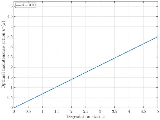
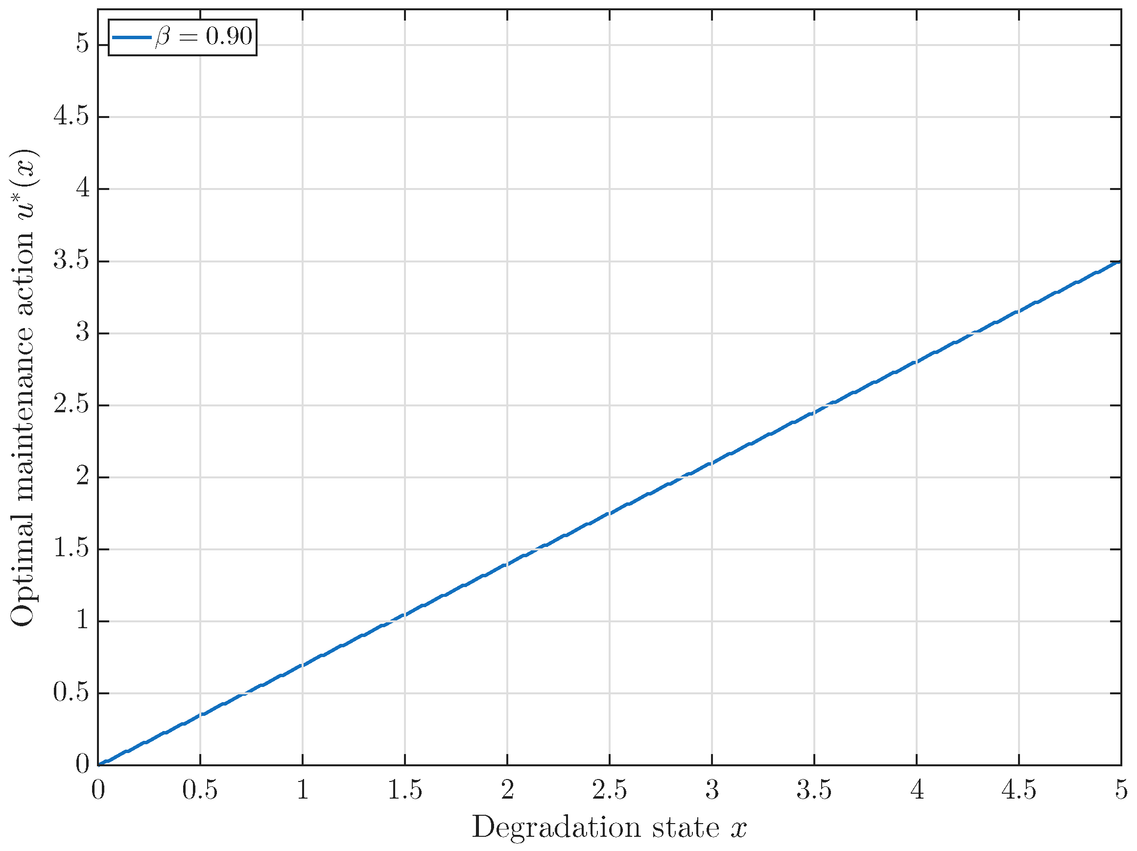
Figure 1 presents the corresponding optimal maintenance policy.

Figure 1. Optimal maintenance policy for the baseline discount factor $\beta =0.90$.

The optimal policy is nondecreasing with respect to the degradation state. For states close to zero, little or no maintenance is optimal. As degradation increases, the optimal maintenance action increases steadily.

The computed actions at several representative states are

$$\begin{array}{cccccc}\hfill u^{*}\left(0\right)& =0,\hfill & \hfill u^{*}\left(1\right)& \approx 0.6944,\hfill & \hfill u^{*}\left(2\right)& \approx 1.3988,\hfill \\ \hfill u^{*}\left(3\right)& \approx 2.0933,\hfill & \hfill u^{*}\left(4\right)& \approx 2.7976,\hfill & \hfill u^{*}\left(5\right)& \approx 3.5020.\hfill \end{array}$$

Thus, the numerical results exhibit a natural preventive-maintenance pattern. When the degradation level is low, the immediate cost of stronger intervention is not justified by the corresponding reduction in future costs. As the system deteriorates, future degradation becomes increasingly costly, and a larger maintenance action becomes optimal.

It is also worth noting that the upper control bound is not active in the baseline computation. Although $u_{max}=5$, the largest optimal action obtained on the state interval is approximately $3.502$. Hence, for the present parameter values, the optimal policy remains strictly below the imposed control constraint.

5.3. Grid-Refinement Analysis

To examine the influence of the numerical discretization, the problem was solved on three successively finer grids,

$$(N_x,N_u)=(101,101),(201,251),(405,505).$$

All computations were performed with $\beta =0.90$ and the same stopping tolerance. The results are presented in Table 1.

Table 1. Grid-refinement results and convergence diagnostics.

${\mathit{N}}_{\mathit{x}}$	${\mathit{N}}_{\mathit{u}}$	Iterations	Final Difference	A Posteriori Bound	Bellman Residual
101	101	122	$1.02035\times {10}^{-5}$	$9.18311\times {10}^{-5}$	$9.18311\times {10}^{-6}$
201	251	122	$1.02037\times {10}^{-5}$	$9.18331\times {10}^{-5}$	$9.18331\times {10}^{-6}$
405	505	122	$1.02038\times {10}^{-5}$	$9.18338\times {10}^{-5}$	$9.18338\times {10}^{-6}$

The number of value iterations is identical for all three discretizations. Moreover, the final successive differences, a posteriori error estimates, and Bellman residuals are nearly unchanged under grid refinement. This indicates that the convergence behavior of the iterative procedure is not sensitive to the selected state and control discretizations.

A more direct assessment of discretization stability is obtained by comparing solutions on consecutive grids. The sup-norm difference between the value functions computed on the first two grids is approximately $2.206\times {10}^{-3},$ whereas the corresponding difference between the two finest grids decreases to $3.558\times {10}^{-4}.$

The maximum difference between the corresponding discrete policies decreases from $3.0\times {10}^{-2}$ to approximately $1.73\times {10}^{-2}.$

These results show that both the value function and the optimal policy stabilize as the grids are refined. In particular, the differences between the value functions obtained on successive grids decrease substantially under refinement. The observed policy differences also decrease, although the policy convergence is affected by the finite resolution of the control grid. The finest grid $(405,505)$ is therefore used in the remaining numerical experiments.

5.4. Influence of the Discount Factor

We next examine the influence of the discount factor on the optimal solution. The numerical problem is solved for

$$\beta \in \{0.70,0.80,0.90,0.95\},$$

using the finest discretization.

The computed value functions increase substantially with the discount factor. For instance, at $x=5$,

$$v^{*}\left(5\right)=41.8268\mathrm{for}\beta =0.70,$$

whereas

$$v^{*}\left(5\right)=103.7804\mathrm{for}\beta =0.95.$$

A similar increase occurs at every selected state. This behavior is expected because a larger discount factor assigns more weight to future maintenance and degradation costs, thereby increasing the total expected discounted cost.

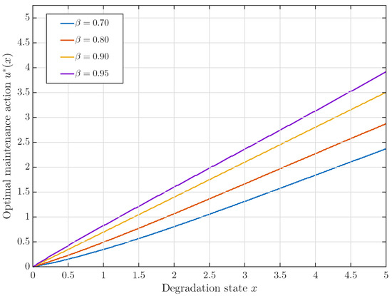
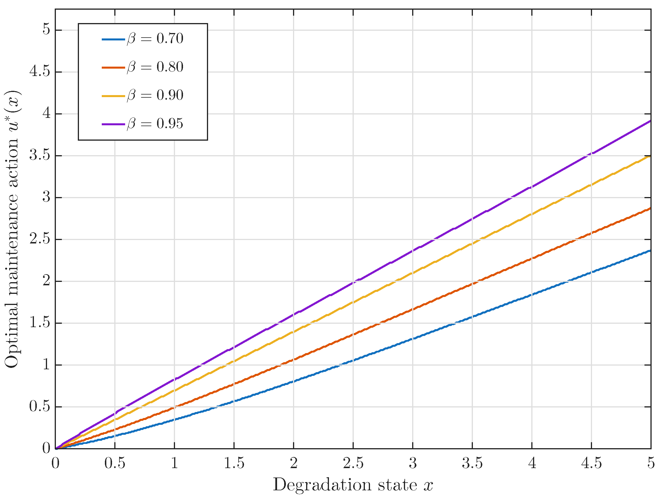
More importantly from the maintenance perspective, the discount factor also affects the optimal maintenance strategy. Figure 2 shows the optimal policies obtained for the four considered discount factors.

Figure 2. Effect of the discount factor on the optimal maintenance policy.

For every fixed degradation state $x>0$, the optimal maintenance action increases with the discount factor. At $x=5$, the computed optimal actions are approximately

$$2.3710,2.8770,3.5020,3.9187,$$

for $\beta =0.70$, $0.80$, $0.90$, and $0.95$, respectively.

This behavior has a natural interpretation. When the discount factor is relatively small, future costs have less influence on the current decision, and the optimal policy favors less intensive maintenance. As $\beta$ increases, future degradation costs become more important. The controller therefore applies stronger maintenance actions in the current period to reduce the expected cost associated with future degradation.

The numerical experiment thus shows that the discount factor affects not only the magnitude of the value function but also the optimal maintenance strategy. A larger discount factor leads to more intensive maintenance at a given degradation level.

For all considered values of $\beta$, the optimal policy remains below the upper bound $u_{max}=5$. Hence, the control constraint is not active on the state interval $[0,5]$ for the parameter configurations considered here.

5.5. Convergence Behavior of Value Iteration

Finally, we examine the convergence behavior of value iteration for different discount factors.

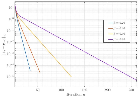
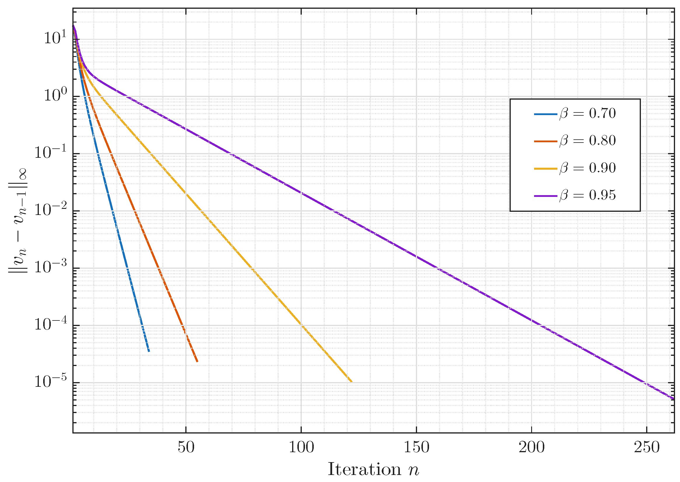
Figure 3 shows the successive differences

$$\parallel v_n-v_{n-1}{\parallel }_{\infty }$$

(12)

on a logarithmic scale.

Figure 3. Convergence histories of value iteration for different discount factors.

For every considered discount factor, the successive differences decrease approximately geometrically after a short initial transient. This behavior is consistent with the contraction property of the discounted Bellman operator.

The number of iterations required to satisfy the prescribed stopping criterion increases significantly with the discount factor. The algorithm terminates after 34 iterations for $\beta =0.70$, 55 iterations for $\beta =0.80$, 122 iterations for $\beta =0.90$, and 262 iterations for $\beta =0.95$.

This behavior is expected because the contraction modulus of the Bellman operator is $\beta$. Consequently, the contraction becomes weaker as $\beta$ approaches one, and more iterations are required to achieve the same prescribed iterative accuracy.

To examine this behavior numerically, we compute the median ratio of consecutive successive differences over the final 20 iterations. The resulting values are

$$0.6996,0.8000,0.9000,0.9500,$$

for $\beta =0.70$, $0.80$, $0.90$, and $0.95$, respectively.

The observed ratios are very close to the corresponding theoretical contraction moduli. Thus, the numerical convergence behavior agrees closely with the contraction estimate established in the theoretical analysis.

5.6. Discussion of the Numerical Results

The numerical experiments illustrate the theoretical properties of the model and provide additional information about the structure of the optimal maintenance strategy. For the baseline parameter configuration, the computed value function increases with the degradation state, while the optimal stationary policy prescribes stronger maintenance actions as degradation increases. At the same time, the upper control bound remains inactive, showing that the computed optimal actions are determined by the balance between maintenance and degradation costs rather than by the imposed action constraint.

The grid-refinement analysis indicates that the numerical approximation stabilizes with respect to refinement of the state and control grids. The differences between solutions obtained on successive grids decrease under refinement, while the convergence diagnostics remain essentially unchanged. This provides numerical evidence that the computed solution is not strongly sensitive to the selected discretization and supports the use of the finest grid in the sensitivity analysis.

The discount-factor experiment shows that placing greater weight on future costs leads to stronger maintenance actions at a given degradation level. It also shows that increasing the discount factor slows the convergence of value iteration. The observed ratios of consecutive iteration differences closely match the corresponding contraction moduli, providing a numerical illustration of the contraction behavior established in the theoretical analysis.

Overall, the numerical results are consistent with the theoretical properties of the discounted stochastic maintenance problem. The computations illustrate the structure of the optimal maintenance policy, the stability of the numerical approximation under grid refinement, and the influence of the discount factor on both the optimal solution and the convergence behavior of value iteration.

6. Conclusions

This paper presented a mathematical analysis of an infinite-horizon discounted stochastic maintenance optimization problem formulated within the framework of dynamic programming. The main contribution is the rigorous analysis of the Bellman operator associated with the proposed maintenance model. It was shown that the operator is well defined on the Banach space of continuous functions, maps this space into itself, and is a contraction. These properties lead directly to the existence and uniqueness of the optimal value function and guarantee the convergence of value iteration.

A further contribution of the paper is the derivation of a priori and a posteriori error estimates. Besides providing theoretical convergence results, these estimates establish practical stopping criteria for the numerical algorithm and therefore create a direct connection between the analytical results and their computational implementation.

The numerical experiments support the theoretical analysis. They demonstrate the stability of the numerical solution under grid refinement, illustrate the dependence of the optimal maintenance policy on the degradation level and the discount factor, and show that the observed convergence rates agree closely with those predicted by the contraction analysis.

The proposed framework combines a rigorous theoretical treatment with a straightforward numerical implementation. Although the model considered here is intentionally simple, the analytical approach can be extended to more general stochastic maintenance optimization problems. Future research may include multidimensional degradation models, state-dependent maintenance costs, and maintenance optimization for systems with multiple interacting components.

References

- Arts, J.; Boute, R.N.; Loeys, S.; van Staden, H.E. Fifty years of maintenance optimization: Reflections and perspectives. Eur. J. Oper. Res. 2025, 322, 725–739. [Google Scholar] [CrossRef] [Scilit]
- Nakagawa, T. Maintenance Theory of Reliability; Springer: London, UK, 2005. [Google Scholar]
- Jardine, A.K.S.; Tsang, A.H.C. Maintenance, Replacement, and Reliability, 2nd ed.; CRC Press: Boca Raton, FL, USA, 2013. [Google Scholar]
- Dekker, R. Applications of maintenance optimization models: A review and analysis. Reliab. Eng. Syst. Saf. 1996, 51, 229–240. [Google Scholar] [CrossRef] [Scilit]
- De Jonge, B.; Scarf, P.A. A review on maintenance optimization. Eur. J. Oper. Res. 2020, 285, 805–824. [Google Scholar] [CrossRef] [Scilit]
- Bellman, R. Dynamic Programming; Princeton University Press: Princeton, NJ, USA, 1957. [Google Scholar]
- Howard, R.A. Dynamic Programming and Markov Processes; MIT Press: Cambridge, MA, USA, 1960. [Google Scholar]
- Puterman, M.L. Markov Decision Processes: Discrete Stochastic Dynamic Programming; John Wiley & Sons: New York, NY, USA, 1994. [Google Scholar]
- Bertsekas, D.P. Dynamic Programming and Optimal Control, 4th ed.; Athena Scientific: Belmont, MA, USA, 2017; Volume I. [Google Scholar]
- Bertsekas, D.P.; Shreve, S.E. Stochastic Optimal Control: The Discrete-Time Case; Academic Press: New York, NY, USA, 1978. [Google Scholar]
- Denardo, E.V. Contraction Mappings in the Theory Underlying Dynamic Programming. SIAM Rev. 1967, 9, 165–177. [Google Scholar] [CrossRef] [Scilit]
- Leppinen, J.; Punkka, A.; Ekholm, T.; Salo, A. An optimization model for determining cost-efficient maintenance policies for multi-component systems with economic and structural dependencies. Omega 2025, 130, 103162. [Google Scholar] [CrossRef] [Scilit]
- Zhang, Z.; Li, H.; Li, T.; Zhang, J.; Si, X. An optimal condition-based maintenance policy for nonlinear stochastic degrading systems. Reliab. Eng. Syst. Saf. 2024, 251, 110349. [Google Scholar] [CrossRef] [Scilit]
- Forootani, A.; Ghaniee Zarch, M.; Tipaldi, M.; Iervolino, R. A stochastic dynamic programming approach for the machine replacement problem. Eng. Appl. Artif. Intell. 2023, 118, 105638. [Google Scholar] [CrossRef] [Scilit]
- Rudin, W. Functional Analysis, 2nd ed.; McGraw–Hill: New York, NY, USA, 1991. [Google Scholar]
- Kreyszig, E. Introductory Functional Analysis with Applications; John Wiley & Sons: New York, NY, USA, 1978. [Google Scholar]
- Boyd, D.W.; Wong, J.S.W. On Nonlinear Contractions. Proc. Am. Math. Soc. 1969, 20, 458–464. [Google Scholar] [CrossRef] [Scilit]
- Kirk, W.A.; Sims, B. Handbook of Metric Fixed Point Theory; Kluwer Academic Publishers: London, UK, 2001. [Google Scholar]
- Granas, A.; Dugundji, J. Fixed Point Theory; Springer: New York, NY, USA, 2003. [Google Scholar]
- Banach, S. Sur les opérations dans les ensambles abstrait et leur application aux équations intégrales. Fundam. Math. 1922, 3, 133–181. [Google Scholar] [CrossRef] [Scilit]
- Atalan, Y. On a new fixed point iterative algorithm for general variational inequalities. J. Nonlinear Convex Anal. 2019, 20, 2371–2386. [Google Scholar] [CrossRef] [Scilit]
- Maldar, S. New parallel fixed point algorithms and their application to a system of variational inequalities. Symmetry 2022, 14, 1025. [Google Scholar] [CrossRef] [Scilit]
- Hacıoğlu, E.; Ertürk, M.; Gürsoy, F.; Milovanović, G.V. Flexible and Efficient Iterative Solutions for General Variational Inequalities in Real Hilbert Spaces. Axioms 2025, 14, 288. [Google Scholar] [CrossRef] [Scilit]
Disclaimer/Publisher’s Note: The statements, opinions and data contained in all publications are solely those of the individual author(s) and contributor(s) and not of MDPI and/or the editor(s). MDPI and/or the editor(s) disclaim responsibility for any injury to people or property resulting from any ideas, methods, instructions or products referred to in the content. |
© 2026 by the authors. Licensee MDPI, Basel, Switzerland. This article is an open access article distributed under the terms and conditions of the Creative Commons Attribution (CC BY) license.