SIR Model with Dependent Infectivity and Death Rates

Abstract

This work constructs, analyzes and simulates a new general SIR epidemiological model for the spread of a generic long-time disease, in which the coefficients of infectivity and death rate are system variables. Diseases, such as COVID-19, have demonstrated clearly that infectivity and death rates can change over time, even for the same variant of the virus, due to vaccination, improved treatments, better analysis, better medications, etc. This motivates us to construct the SIR-ID model for a generic disease in which the rate coefficients are state variables as a part of the systems’s evolution in time. The model consists of a coupled system of five differential equations, where the equations for the infectivity and death rate have general source functions. The analysis shows the existence, positivity and boundedness of the solutions. A discussion of the Endemic (EE) and Disease-Free (DFE) equilibria and their stability is provided. A bifurcation analysis of the DFE and EE is conducted, as well as a sensitivity analysis. Then, computer simulations depict two typical cases of dynamic behavior, one when the DFE is stable and attracting, and one in which the EE is stable and attracting. These also show the way the system approaches the steady states.

1. Introduction

We develop, analyze and simulate the SIR-ID model, a new extended version of the standard SIR model for the spread of a communicable disease, in which both infectivity and death rates are system variables. The motivation for including system-dependent infectivity and death rates comes from observations on the evolution of the COVID-19 epidemic. It seems that by allowing for such extension of the basic SIR model, a more realistic and more accurate description is provided for certain long-lasting diseases. The model here is generic and needs to be updated with infectivity and death rate source functions, that are tailored to each specific disease. In part, this model may have more accurate predictions than models with curve-fitting of infectivity and death-rate.

This work considerably extends [1], which constructs, analyzes and simulates the SIR-IH model, a modified SIR model in which the infectivity rate and hospitalization ratio are system variables. There, the infective population was split into those with a mild version of the disease and those needing hospitalization, with simple ad hoc source terms. Here, we develop a general SIR-ID model with general source functions. The aim in [1] was to develop a mathematical tool that would allow the authorities to estimate the needed hospitalization resources in case of a long-time mass disease. Here, we consider a substantially more general model. This concept of having some of the system coefficients as state variables was already considered in [2] as well as in [1].

A recent work, [3], constructed an epidemiological model for cancer in which, to account for the adaptive nature of the tumor’s PD-L1 expression, the authors introduced an additional ordinary differential equation governing the dynamics of the state variable $\epsilon$, which describes the rate of change in the tumor PD-L1 expression level over time.

A basic and comprehensive review of the SIR-type compartmental models can be found in the survey by Heathcote in [4]. We note that the literature on various aspects of SIR models is very large, and in addition to [4], many references can be found in [5,6] and also those in [7].

It is known, see, e.g., [8,9,10] and the references therein, that the death rate for COVID-19 did vary over time, even for a the same variant. Factors such as vaccination, new treatments (antiviral and steroids), and post-infection immunity evolved alongside the virus, altering the infectivity rate and death rate of infected individuals. These rates reflect the complex interaction between a variant’s virulence and the body’s and health responses. For example, vaccination significantly reduced severe outcomes and deaths, even for highly transmissible variants such as the Omicron [10]. Development and deployment of antivirals (such as Paxlovid) lowered death rates [9]. Repeated infections built up population-level immunity, making subsequent waves less deadly [11]. These are some examples of the many factors that affected the death and infectivity rates for COVID-19. These observations, which apply to most other longer term contagious diseases, and noting that similar factors affect the infectivity rate, motivate our general model.

In later stages of this work, we intend to attempt to compare the predictions of this model with those of a model in which the infectivity and death rate were curve-fitted from real data. However, currently, we are looking in the literature for a paper of this type.

Following this introduction, we derive the model in detail in Section 2. There, the compartmental flow chart and the model equations can be found. The model consists of five rate equations, the basic equation of the SIR model for the Susceptibles, Infected and Recovered, and the addition of two equations for the death rate due to the disease and the infectivity rate. As noted above, the novelty in this work lies in the introduction of differential equations for the disease-related death rate $\tilde{\alpha }$ and the infectivity rate $\tilde{\beta }$, which are treated as unknowns, with source functions ${\Psi }_{\alpha }$ and ${\Psi }_{\beta }$ that are very general. However, these variables are constrained to avoid unreasonable values that the differential equations may produce. Since each specific disease has its own dynamics, the source functions ${\Psi }_{\alpha }$ and ${\Psi }_{\beta }$ need to be tailored to each case based on observations, if possible. Related explanations can be found in Remarks 1 and 2.

Section 3 establishes the positivity and boundedness of the solutions, which makes them biologically viable, and then states the theorem on the global existence of the solution.

The steady states of the system and their stability are studied in Section 4. The Disease-Free Equilibrium (DFE) is described in Theorem 3, and a sensitivity analysis conducted in Section 4.2, shows-that the system is most sensitive to the infectivity $\beta$. The global stability of the DFE, when the stability number ${\mathcal{R}}_0<1$, is established in Section 4.3. Section 4.4 describes, in Theorem 5, the transcritical bifurcation of the steady states when ${\mathcal{R}}_0=1$. Result 1 and Theorem 6 characterize the Endemic Equilibrium (EE) when ${\mathcal{R}}_0>1$. Finally, Theorem 7 states that the system does not have Hopf bifurcations, hence no oscillations.

Section 5 describes a simple explicit finite difference algorithm for the computer simulations of the model and shows two typical solutions. The first depicts the DFE, with system constants that make it stable and attracting. The second simulation is in the case when the DFE is unstable, and then the EE is stable and attracting. Furthermore, the simulations show the system’s approach to these steady states. To obtain confidence in the simulations, Section 6 presents a numerical argument for the convergence of the numerical method. The conclusions of the work and some ideas for future study can be found in Section 7.

2. The Model

We present a general SIR model of disease transmission, modified so it includes dependent rates of infectivity and death. We use the terminology of a generic disease in a large city in which the disease is spreading. Modifications to the model for a specific disease and location need to be tailored to the disease. We follow, in part, the presentation and ideas in [1].

We deal with whole populations, do not consider their spatial spread, and assume that the populations are large enough to justify the use of ordinary differential equations (ODEs). As  noted in the introduction, we describe the dynamics of three populations consisting of individuals: susceptible (S), infected (I), and  recovered (R). These are functions of time, and the rate of change of each population is described in the model. For simplicity, we consider the time unit to be a day. The novelty in this work is the assumption that the disease-induced death rate function $\left(\alpha =\alpha \left(t\right)\right)$ and the infectivity rate function $\left(\beta =\beta \left(t\right)\right)$ are dependent variables. The infectivity rate function $\beta$ is the probability that one susceptible person who comes into contact with one infected becomes sick. This measures how rapidly the disease may spread.

We assume that the death rate function $\alpha$ and the infectivity rate function $\beta$ are only mildly related. We use a differential equation for each one that depends on the infected and recovered populations. Moreover, we assume that the fraction r of those who have recovered can lose their immunity and be reinfected.

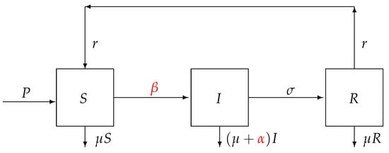
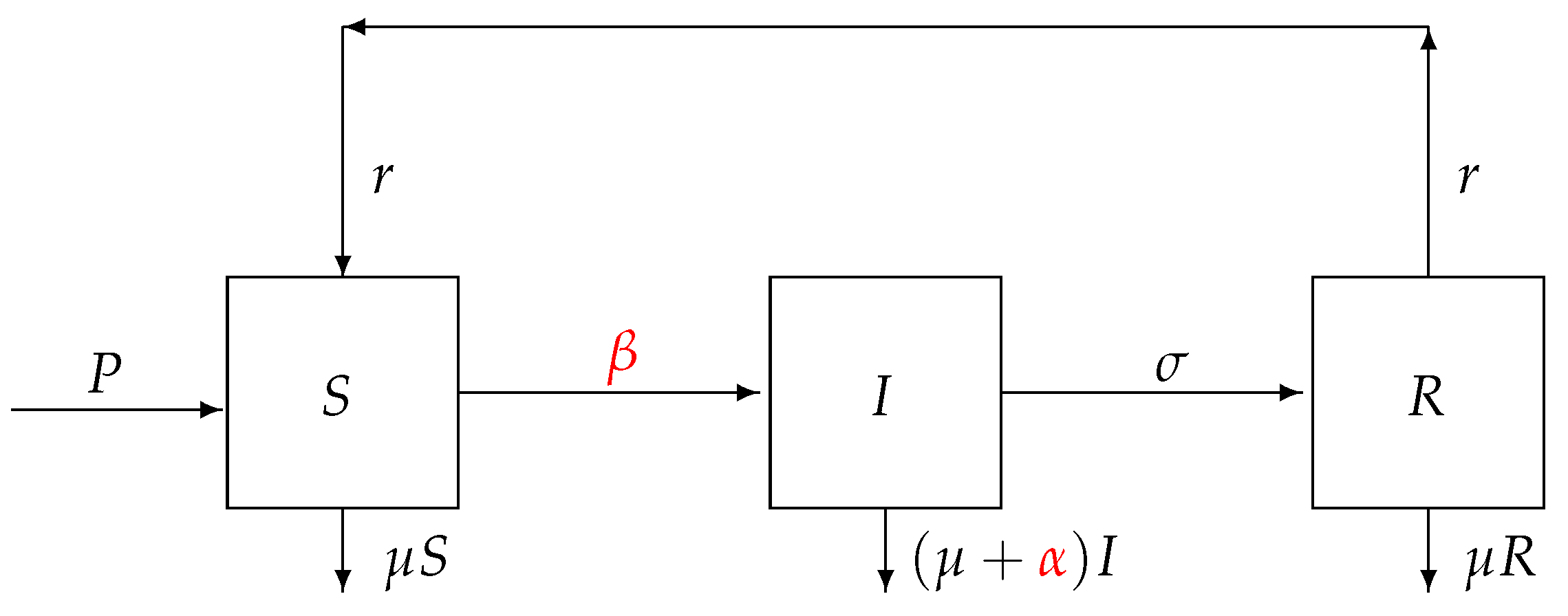
The compartmental structure of the model, see, e.g., [7], is depicted in Figure 1.

Figure 1. Compartmental structure and flow chart; $\alpha =\alpha \left(t\right)$ and $\beta =\beta \left(t\right)$ (red) are dependent variables, too.

The susceptible population $S=S\left(t\right)$ consists of all individuals who are healthy and can become sick. The infected population $I=I\left(t\right)$ consists of individuals infected with the disease. Individuals in $I\left(t\right)$ may or may not present clinical symptoms of the disease. The population $R=R\left(t\right)$ denotes those who recovered from the disease.

We denote by $P\left(t\right)$ the net number of susceptible individuals that are added to the city per day, either by birth or outside arrivals. We let $\mu (1/\mathrm{day})$ denote the death rate in the absence of the disease, and then the death rate for the infected is $\mu +\alpha (1/\mathrm{day})$.

The disease recovery constant is $\sigma$ and the number of recovered (per day) is $\sigma I$. We let $r\in (0,1]$ denote the fraction of recovered that become susceptible again. For the sake of simplicity, we assume that $\sigma$ and r are constants. It is straightforward to make them dependent variables, however, at the expense of making the model more complex.

Remark 1.

The equations for the changes in α and β are of the general form

$${\displaystyle \frac{d\alpha }{dt}}={\Psi }_{\alpha }(I,R,\alpha ,\beta ),{\displaystyle \frac{d\beta }{dt}}={\Psi }_{\beta }(I,R,\alpha ,\beta ),$$

(1)

for given source functions ${\Psi }_{\alpha }$ and ${\Psi }_{\beta }$, which need to be established for each disease, based on field data. However, in this work, we just impose mathematical constraints on these functions. Also, these may be set as set-inclusions, which we will comment on in Remark 2, and are also likely to depend on the disease history.

For simplicity and lack of specific information, in the simulations in Section 5, we assume that

$${\Psi }_{\alpha }(I,R,\alpha ,\beta )={\delta }^{+}I-{\delta }^{-}\alpha R,{\Psi }_{\beta }(I,R,\alpha ,\beta )={\gamma }^{+}I-{\gamma }^{-}\beta R.$$

Here, ${\delta }^{+},{\delta }^{-},{\gamma }^{+},{\gamma }^{-}$ are positive constants, to be determined from field data. The dependence on R is due to population immunity from prior infections, while the dependence on I seems to be natural.

Since $\alpha$ and $\beta$ are dependent variables, we need to make sure that their values remain within reasonable intervals, no matter what the populations are. To that end, let $0<{\alpha }_{-}<{\alpha }_{+}$ and $0<{\beta }_{-}<{\beta }_{+}\le 1$ be the limits for the allowed values of $\alpha$ and $\beta$, respectively, and we want to guarantee that for $0\le t\le T$,

$$\alpha \left(t\right)\in [{\alpha }_{-},{\alpha }_{+}],\beta \left(t\right)\in [{\beta }_{-},{\beta }_{+}].$$

(2)

To that end, we introduce the restriction or cutoff operators ${\Phi }_{\alpha },{\Phi }_{\beta }$, acting on $s\in \mathbb{R}$, as follows,

$${\Phi }_{\alpha }\left(s\right)=\left\{\begin{array}{cc}{\alpha }_{-},\hfill & s\le {\alpha }_{-},\hfill \\ s,\hfill & {\alpha }_{-}<s<{\alpha }_{+},\hfill \\ {\alpha }_{+}\hfill & s\ge {\alpha }_{+}.\hfill \end{array}\right.{\Phi }_{\beta }\left(s\right)=\left\{\begin{array}{cc}{\beta }_{-},\hfill & s\le {\beta }_{-},\hfill \\ s,\hfill & {\beta }_{-}<s<{\beta }_{+},\hfill \\ {\beta }_{+}\hfill & s\ge {\beta }_{+},\hfill \end{array}\right.$$

(3)

Both operators are bounded, piecewise linear and Lipschitz continuous, and are used in the model below.

The total living population, at time t, is given by

$$N\left(t\right)=S\left(t\right)+I\left(t\right)+R\left(t\right),$$

(4)

and is not assumed to be constant.

These assumptions lead to the following mathematical model for SIR-ID, a modified SIR disease dynamical system with system-dependent infectivity and death rates.

Model 1.

SIR-ID Find five functions$(S,I,R,\tilde{\alpha },\tilde{\beta })$, defined on $[0,T]$, such that the following equations hold, for $0<t\le T$:

$$\begin{array}{cc}\hfill {\displaystyle \frac{dS}{dt}}& =P-\beta I{\displaystyle \frac{S}{N}}-\mu S+rR,\hfill \end{array}$$

(5)

$$\begin{array}{cc}\hfill {\displaystyle \frac{dI}{dt}}& =\beta I{\displaystyle \frac{S}{N}}-(\mu +\alpha +\sigma )I,\hfill \end{array}$$

(6)

$$\begin{array}{cc}\hfill {\displaystyle \frac{dR}{dt}}& =\sigma I-\mu R-rR,\hfill \end{array}$$

(7)

$$\begin{array}{cc}\hfill {\displaystyle \frac{d\tilde{\alpha }}{dt}}& ={\Psi }_{\alpha },\hfill \end{array}$$

(8)

$$\begin{array}{cc}\hfill {\displaystyle \frac{d\tilde{\beta }}{dt}}& ={\Psi }_{\beta },\hfill \end{array}$$

(9)

where

$$\alpha \left(t\right)={\Phi }_{\alpha }\left(\widetilde{\alpha \left(t\right)}\right),\beta \left(t\right)={\Phi }_{\beta }\left(\widetilde{\beta \left(t\right)}\right)$$

(10)

and N is given in (4). The initial conditions are

$$S\left(0\right)=S_0,I\left(0\right)=I_0,R\left(0\right)=R_{init},\alpha \left(0\right)={\alpha }_0,\beta \left(0\right)={\beta }_0.$$

(11)

Equations (5)–(7) form the usual SIR model. The mathematical assumptions on the source functions ${\Psi }_{\alpha }$ and ${\Psi }_{\beta }$ are specified in the theorems in Section 3. Moreover, $\tilde{\alpha }$ and $\tilde{\beta }$ are the unrestricted auxiliary dependent variables. Everywhere below, we refer to the restricted variables $\alpha$ and $\beta$ as the disease-induced death and infectivity rates, respectively. We denote by $R_{init}$ the initial value of R, since in mathematical epidemiology ${\mathcal{R}}_0$ usually denotes the basic stability number, or the basic reproduction number, see [4] and Section 4.

Furthermore, $S_0>0$ is the initial population before the outbreak of the disease, and $I_0\ge 0$, $R_{init}\ge 0$ are the initial populations at $t=0$. Additionally, $\alpha \left(0\right)={\alpha }_0\in [{\alpha }_{-},{\alpha }_{+}]$ is the initial disease-induced death rate and $\beta \left(0\right)={\beta }_0\in [{\beta }_{-},{\beta }_{+}]$ is the initial infectivity rate.

In practice, one typically assumes that initially $S_0=N\left(0\right)>0$, so that at the outbreak, the population is only of susceptibles, and all the other populations vanish. However, for the sake of generality, we allow for them to be nonnegative but satisfying $N\left(0\right)=S_0+I_0+R_{init}$, so that (4) holds at $t=0$.

Next, Equations (8) and (9) represent the general form of the dynamics of the death rate and infectivity. The general assumptions on the functions are presented in Section 3. As was noted above, in the simulations section for simplicity and lack of specific information, we assume that

$${\Psi }_{\alpha }(I,R,\alpha ,\beta )={\delta }^{+}I-{\delta }^{-}\alpha R,{\Psi }_{\beta }(I,R,\alpha ,\beta )={\gamma }^{+}I-{\gamma }^{-}\beta R.$$

We assume that the infectivity of the disease increases with the number of infected, I, as the disease agent has more options to grow and possibly mutate, and decreases with the number of recovered, as more individuals are immune. It may be of interest to study the question of the form of ${\Psi }_{\alpha }$ and ${\Psi }_{\beta }$ in the future, as it deserves a thorough investigation.

The following remark can be found in [1].

Remark 2.

Instead of using the restriction operators ${\Phi }_{\alpha },{\Phi }_{\beta }$, we may use the notion of the subdifferential. To that end, we let $I_{\alpha },I_{\beta }$ be the indicator functions of $[{\alpha }_{-},{\alpha }_{+}]$ and $[{\beta }_{-},{\beta }_{+}]$, that is, $I_{\alpha }\left(\alpha \right)=0$ if $\alpha \in [{\alpha }_{-},{\alpha }_{+}]$ and $I_{\alpha }=+\infty$ otherwise, and similarly, $I_{\beta }\left(\beta \right)=0$ if $\beta \in [{\beta }_{-},{\beta }_{+}]$ and $I_{\beta }=+\infty$ otherwise. Let $\partial I_{\alpha },\partial I_{\beta }$ be the subdifferentials,

$$\partial I_{\alpha }\left(s\right)=\left\{\begin{array}{cc}(-\infty ,0],\hfill & s={\alpha }_{-},\hfill \\ 0\hfill & {\alpha }_{-}<s<{\alpha }_{+},\hfill \\ [0,\infty )\hfill & s={\alpha }_{+},\hfill \end{array}\right.$$

and similarly for $\partial I_{\beta }$, with β replacing α.

Then, instead of using the restriction operators, we may use the set-valued inclusions for α and β, which are

$${\displaystyle \frac{d\alpha }{dt}}\in {\Psi }_{\alpha }(I,R,\alpha ,\beta )-\partial I_{\alpha }\left(\alpha \right),{\displaystyle \frac{d\beta }{dt}}\in {\Psi }_{\beta }(I,R,\alpha ,\beta )-\partial I_{\beta }\left(\beta \right).$$

The subdifferentials guarantee that the variables cannot leave the designated intervals.

A summary of the definitions of the model parameters is given in Table 1.

Table 1. Symbols and description of parameters used in the model; the dimensional quantities are per day.

Parameter	Description
P	recruitment rate of susceptible individuals
$\alpha$	(restricted) disease-induced death rate (10)
$\beta$	(restricted) infectivity rate (10)
$\mu$	natural death rate
$\sigma$	recovery rate of infected
r	loss of immunity rate of recovered
${\delta }^{-},{\delta }^{+}$	disease-induced death limits
${\gamma }^{-},{\gamma }^{+}$	infectivity limits
${\alpha }_{-},{\alpha }_{+}$	restriction intervals values for $\tilde{\alpha }$
${\beta }_{-},{\beta }_{+}$	restriction intervals values for $\tilde{\beta }$
$S_0,I_0,R_{init}$	initial populations
${\alpha }_0,{\beta }_0$	initial rates

3. Positivity, Boundedness and Existence

This section establishes the nonnegativity, boundedness and existence of global solutions to the model. These are important factors in ensuring that the model makes sense both mathematically and biologically. We note that the local existence is guaranteed by the general theory of dynamical systems, since the system is locally Lipschitz continuous.

Outside of this section, we take the recruitment rate P of susceptible individuals to be constant with respect to time. However, here, for the sake of generality, we allow P to be a bounded, Lipschitz continuous and nonnegative function of time, with upper bound $P_{\max }$.

To proceed, we need the following assumptions on the functions ${\Psi }_{\alpha }$ and ${\Psi }_{\beta }$:

Assumption 1.

The source functions ${\Psi }_{\alpha }={\Psi }_{\alpha }(I,R,\tilde{\alpha },\tilde{\beta })$ and ${\Psi }_{\beta }$$={\Psi }_{\beta }(I,R,\tilde{\alpha },\tilde{\beta })$ are locally Lipschitz continuous. That is, there exist two positive constants $C_{\alpha }^{\ast }$ and $C_{\beta }^{\ast }$, such that in the box

$$B_b=\{(I,R,\tilde{\alpha },\tilde{\beta })\in {\mathbb{R}}_{+}^4:\left|I\right|,\left|R\right|,|\tilde{\alpha }|,|\tilde{\beta }|\le b^{\ast }\}$$

where $C_{\alpha }^{\ast }$ and $C_{\beta }^{\ast }$ depend on $b^{\ast }$, which are such that

$$\begin{gathered} |{\Psi }_{\alpha }(I_1,R_1,{\tilde{\alpha }}_1,{\tilde{\beta }}_1)-{\Psi }_{\alpha }(I_2,R_2,{\tilde{\alpha }}_2,{\tilde{\beta }}_2)| \le C_{\alpha }^{\ast }\left(\right|I_1-I_2|+|R_1-R_2| \\ +|{\tilde{\alpha }}_1-{\tilde{\alpha }}_2|+|{\tilde{\beta }}_1-{\tilde{\beta }}_2\left|\right), \end{gathered}$$

and similarly for ${\Psi }_{\beta }$. Moreover, we assume that

$${\Psi }_{\alpha }(I,R,\tilde{\alpha },\tilde{\beta })\ge -{\delta }^{+}\tilde{\alpha }R,{\Psi }_{\beta }(I,R,\tilde{\alpha },\tilde{\beta })\ge -{\delta }^{+}\tilde{\beta }R,$$

(12)

for all $(I,R,\tilde{\alpha },\tilde{\beta })\in {\mathbb{R}}_{+}^4$.

We note that these conditions hold for the choice of ${\Psi }_{\alpha }$ and ${\Psi }_{\beta }$ in the simulations.

Theorem 1 (Positivity and boundedness).

Let $S_0>0, I_0\ge 0,$ and $R_{init}\ge 0$, and assume that $\Psi \alpha$ and ${\Psi }_{\beta }$ satisfy Assumptions 1. If $z\left(t\right)=\left(S\right(t),I(t),R(t\left)\right)$ is any solution to the system, then all of the components of z are nonnegative and uniformly bounded on each interval [0, T] on which they exist, for $0<T\le \infty$. Then, for $0\le t\le T$,

$$0\le S\left(t\right),I\left(t\right),R\left(t\right)\le N_0+{\displaystyle \frac{P_{max}}{\mu }}$$

where $0\le P\left(t\right)\le P_{\max }$.

We note that this estimate is on $[0,\infty )$, and clearly $\alpha ,\beta$ are bounded and positive.

Proof. 

We first assume, in addition, that $I_0>0$ and $R_{init}>0$, and because of the continuity of the solutions, there exists a time interval $[0,T^{\ast }]$, with $T^{\ast }>0$, such that $S\left(t\right),I\left(t\right),R\left(t\right)>0$ for $0\le t<T^{\ast }$. Let $0<t<T<T^{\ast }$. Then, since $0<I,N$ and $I/N<1$, it follows from (5) and (2) that

$${\displaystyle \frac{dS}{dt}}=P-{\displaystyle \frac{\beta IS}{N}}-\mu S+rR\ge -\left({\displaystyle \frac{\beta I}{N}}+\mu \right)S\ge -({\beta }_{+}+\mu )S.$$

Using the separation of variables and integration on $[0,t]$ together with the initial conditions, we obtain

$$S\left(t\right)\ge S_0{e}^{-({\beta }_{+}+\mu )t}>0,$$

since $S_0>0$. Thus, the solution is positive for all $0<t\le T$. Similarly, from (5) and (6), we have

$$\begin{gathered} I\left(t\right)\ge I_0{e}^{-(\mu +{\alpha }_{+}+\sigma )t}\ge 0, \\ R\left(t\right)\ge R_{init}{e}^{-(\mu +r)t}\ge 0. \end{gathered}$$

Consequently, since $0<{\alpha }_{-}\le \alpha \le {\alpha }^{+}$ and similarly for $\beta$, the solution z is nonnegative on $[0,T]$, for all T for which the solution exists.

We note that the last two estimates are positive, unless $I_0=R_{init}=0$. These inequalities allows us to remove the restriction $T<T^{\ast }$ and, also using continuity, we may assume that $I_0,R_{init}\ge 0$. This means that the system will be nonnegative on every interval on which it exists. Moreover, we have $S\left(t\right)+I\left(t\right)+R\left(t\right)=N\left(t\right)>0$.

Next, we show the boundedness of the solutions. By adding Equations (5)–(7) and using (4), we find

$${\displaystyle \frac{dN}{dt}}=P-\mu N-\alpha I.$$

Hence,

$${\displaystyle \frac{dN}{dt}}\le P_{\max }-\mu N.$$

Next, we rearrange and use the usual manipulations to get

$$\begin{array}{c}\hfill 0<N\left(t\right)\le N_0+{\displaystyle \frac{P_{max}}{\mu }},\end{array}$$

showing $N\left(t\right)$ is bounded from above. Since N is bounded and each of its components (S, I, R) are nonnegative, we have that all of these components are bounded as well. This completes the proof of boundedness of the populations.

Furthermore, because of the cutoff functions ${\Phi }_{\alpha }$ and ${\Phi }_{\beta }$, we know that $\alpha ,\beta$ are nonnegative and bounded. For the sake of completeness, we show that $\widetilde{\alpha \left(t\right)}$ and $\widetilde{\beta \left(t\right)}$ are also positive and bounded on every finite time interval. First, we have the initial conditions of ${\tilde{\alpha }}_0,{\tilde{\beta }}_0>0$. Using Equation (8) and the upper bound for R, and Assumption 1, we obtain

$${\displaystyle \frac{d\tilde{\alpha }}{dt}}={\Psi }_{\alpha }\ge -{\delta }^{+}\tilde{\alpha }R\ge -{\delta }^{+}\tilde{\alpha }(N_0+P_{max}/\mu ).$$

Using separation of variables, integration on $[0,t]$, and the initial conditions, we obtain

$$\tilde{\alpha }\left(t\right)\ge {\tilde{\alpha }}_0{e}^{-{\delta }^{+}(N_0+P_{max}/\mu )t}>0.$$

Thus, $\tilde{\alpha }\left(t\right)>0$ on the interval $[0,t]$, since ${\tilde{\alpha }}_0>0$, and it extends to $[0,T]$. Now, for an upper bound, we take the same Equation (8) and find

$${\displaystyle \frac{d\tilde{\alpha }}{dt}}\le \left|{\Psi }_{\alpha }\right|\le C_{\alpha }^{\ast }\left(b^{\ast }\right)b^{\ast },$$

where we may choose $b^{\ast }=N_0+P_{max}/\mu$.

Again using separation of variables and integrating both sides on $[0,T]$ gives

$$\tilde{\alpha }\left(t\right)\le {\tilde{\alpha }}_0+C_{\alpha }^{\ast }\left(b^{\ast }\right)(N_0+P_{max}/\mu )T.$$

So, we have $\tilde{\alpha }\left(t\right)$ bounded from above of finite T. We follow similar steps for $\tilde{\beta }\left(t\right)$ and get the following two inequalities:

$$\begin{array}{c}\hfill 0\le {\tilde{\alpha }}_0+C_{\alpha }^{\ast }\left(b^{\ast }\right)(N_0+P_{max}/\mu )T,\\ \hfill 0\le {\tilde{\beta }}_0+C_{\beta }^{\ast }\left(b^{\ast }\right)(N_0+P_{max}/\mu )T.\end{array}$$

Thus, these variables are also nonnegative and bounded on every finite time interval $[0,T]$.    □

In addition to proving that the solutions are positive and bounded, we need to establish their global existence. Using the estimates above, having bounded parameters, and knowing that the right-hand-sides of the system are Lipschitz, we infer the existence of a unique solution from standard results for dynamical system (see [12]).

Let $\mathit{x}=\mathit{x}\left(t\right)={(S,I,R,\tilde{\alpha },\tilde{\beta })}^T$, then the model can be written in the condensed form

$${\displaystyle \frac{d\mathit{x}}{dt}}=\mathit{F}(\mathit{x},t),$$

(13)

where

$$\mathit{F}=\left[\begin{array}{c}P-\beta I{\displaystyle \frac{S}{N}}-\mu S+rR\\ \beta I{\displaystyle \frac{S}{N}}-(\mu +\alpha +\sigma )I\\ \sigma I-\mu R-rR\\ {\delta }^{+}I-{\delta }^{-}\tilde{\alpha }R\\ {\gamma }^{+}I-{\gamma }^{-}\tilde{\beta }R\end{array}\right].$$

(14)

Here, $\alpha \left(t\right)={\Phi }_{\alpha }\left(\widetilde{\alpha \left(t\right)}\right),\beta \left(t\right)={\Phi }_{\beta }\left(\widetilde{\beta \left(t\right)}\right)$. It follows from the estimates in Theorem 1 that, for $0<T<\infty$,

$$\left|\right|\mathit{x}\left(t\right)\left|\right|\le L(N_0,P,T),$$

where L depends only on $N_0,P,T$ and the system parameters.

Remark 3.

We note that the bound $L=L(N_0,P,T)$ depends on T via the dependence of  $\tilde{\alpha }$ and $\tilde{\beta }$ on T. This restricts the existence of the solution $\mathit{x}\left(t\right)$ to every finite time interval $[0,T]$ for $T<\infty$. However, even when $\tilde{\alpha }$ or $\tilde{\beta }$ tend to infinity, α and β remain bounded and, therefore, the solution $\left(S\right(t),I(t),R(t\left)\right)$ exists on the interval $[0,\infty )$.

We summarize our results as follows.

Theorem 2 (Existence and uniqueness). 

Let $S_0>0,I_0\ge 0$, $R_{init}\ge 0$,  ${\alpha }_0\in [{\alpha }_{-},{\alpha }_{+}]$, ${\beta }_0\in [{\beta }_{-},{\beta }_{+}]$, Assumption 1 hold, and let all the coefficients be positive constants. Then, there exists a unique solution to Model 1on every time interval $[0,T]$ for $T<\infty$. Furthermore, the solution $\left(S\right(t),I(t),R(t\left)\right)$ exists on the interval $[0,\infty )$.

Proof. 

It is straightforward to show that given bounded coefficients and functions (see Theorem 1), the system is locally Lipschitz continuous. Then, it follows from the estimates above that it is Lipschitz on every finite time interval. Therefore, the result follows from standard results for dynamical systems (see, e.g.,  [12]).    □

4. Steady States

This section studies the equilibrium points of the system and their stability. We have the Disease-Free Equilibrium (DFE) and the Endemic Equilibrium (EE). We assume that $P>0$ is constant, and denote the steady states as follows: $\overline{S},\overline{I},\overline{R},\overline{\alpha },\overline{\beta }$. We first compute the Jacobian and then the eigenvalues of the system, thus establishing the stability of the steady states.

To compute the Jacobian, we find in turn the partial derivatives with respect to S, I and R in Equations (5)–(7). We note that since $N=S+I+R$:

$${\displaystyle \frac{\partial (S/N)}{\partial S}}={\displaystyle \frac{I+R}{N^2}},{\displaystyle \frac{\partial (I/N)}{\partial I}}={\displaystyle \frac{S+R}{N^2}},{\displaystyle \frac{\partial (1/N)}{\partial R}}=-{\displaystyle \frac{1}{N^2}}.$$

For simplicity, we removed the bars in the following. The Jacobian of the right-hand-side of (5)–(7) has the form

$$J_{\mathbf{f}}(S,I,R):=\left[\begin{array}{ccc}-\mu +\beta I{\displaystyle \frac{I+R}{N^2}}& -\beta \left({\displaystyle \frac{S}{N}}-{\displaystyle \frac{SI}{N^2}}\right)& r+\beta I{\displaystyle \frac{SI}{N^2}}\\ \beta I{\displaystyle \frac{I+R}{N^2}}& \beta \left({\displaystyle \frac{S}{N}}-{\displaystyle \frac{SI}{N^2}}\right)-(\mu +\alpha +\sigma )& -\beta {\displaystyle \frac{SI}{N^2}}\\ 0& \sigma & -(\mu +r)\end{array}\right].$$

(15)

Next, we consider the equilibrium points and their stability.

4.1. Disease-Free Equilibrium

We begin with the DFE, which is $(\overline{S},0,0)$, i.e., a boundary equilibrium for all parameter values

$${\mathfrak{E}}^0:=(S^0,I^0,R^0):=\left({\displaystyle \frac{P}{\mu }},0,0\right).$$

We have the following result:

Theorem 3.

The equilibrium ${\mathfrak{E}}^0$ is

• asymptotically stable when

  $$\beta <\mu +\alpha +\sigma ;$$

  (16)
• unstable for

  $$\beta >\mu +\alpha +\sigma .$$

  (17)

Proof. 

It follows from (15) that at ${\mathfrak{E}}^0$,

$$J_{\mathbf{f}}\left({\mathfrak{E}}^0\right)=\left[\begin{array}{ccc}-\mu & -\beta & r\\ 0& \beta -(\mu +\alpha +\sigma )& 0\\ 0& \sigma & -(\mu +r)\end{array}\right].$$

The characteristic polynomial is

$${\chi }_{{\mathfrak{E}}^0}\left(z\right):=det(z{I}_3-J_{\mathbf{f}}\left({\mathfrak{E}}^0\right))=(z+\mu )\left(z-\beta +(\mu +\alpha +\sigma )\right)(z+\mu +r).$$

Clearly, $J_{\mathbf{f}}\left({\mathfrak{E}}^0\right)$ has the eigenvalues

$${\lambda }_1:=-\mu ,{\lambda }_2:=\beta -(\mu +\alpha +\sigma ),{\lambda }_3:=-(\mu +r).$$

Thus, in the first case, (16), $J_{\mathbf{f}}\left({\mathfrak{E}}^0\right)$ is a stable matrix, in the second, (17), it is unstable.    □

In the critical case, i.e., when

$$\beta =\mu +\alpha +\sigma ,$$

(18)

the Jacobian $J_{\mathbf{f}}\left({\mathfrak{E}}^0\right)$ has two negative eigenvalues and zero as the third eigenvalue. We have the following equivalence:

$$\beta =(\mu +\alpha +\sigma )⟺{\displaystyle \frac{\beta }{\mu +\alpha +\sigma }}=1.$$

Therefore, it is natural to identify the fraction on the right-hand-side with the basic reproduction number ${\mathcal{R}}_0$ see, e.g., [13,14,15]. To prove that this is indeed valid, we rewrite system (5)–(7) as

$$(S^{\prime },I^{\prime },R^{\prime })=\mathcal{F}(S,I,R)-\mathcal{V}(S,I,R),$$

where

$$\mathcal{F}(S,I,R):=\left[\begin{array}{c}0\\ \beta I{\displaystyle \frac{S}{N}}\\ 0\end{array}\right]\mathrm{and}\mathcal{V}(S,I,R):=\left[\begin{array}{c}-P+\beta I{\displaystyle \frac{S}{N}}-\mu S-rR,\\ -\beta I{\displaystyle \frac{S}{N}}+(\mu +\alpha +\sigma )I\\ \sigma I-\mu R-rR\end{array}\right].$$

Then, we have the two Jacobians evaluated at the equilibrium ${\mathfrak{E}}^0$,

$$F:={\left[\begin{array}{ccc}0& 0& 0\\ \beta I{\displaystyle \frac{N-S}{N^2}}& \beta {\displaystyle \frac{S}{N}}-\beta I{\displaystyle \frac{S}{N^2}}& 0\\ 0& 0& 0\end{array}\right]}_{{\mathfrak{E}}^0}=\left[\begin{array}{ccc}0& 0& 0\\ 0& \beta & 0\\ 0& 0& 0\end{array}\right],$$

and

$$V:={\left[\begin{array}{ccc}\beta I{\displaystyle \frac{N-S}{N^2}}+\mu & \beta {\displaystyle \frac{S}{N}}-\beta I{\displaystyle \frac{S}{N^2}}& \rho \\ 0& \mu +\alpha +\sigma & 0\\ 0& -\sigma & \mu +\rho \end{array}\right]}_{{\mathfrak{E}}^0}=\left[\begin{array}{ccc}0+\mu & \beta & \rho \\ 0& \mu +\alpha +\sigma & 0\\ 0& -\sigma & \mu +\rho \end{array}\right],$$

giving

$$V^{-1}={\displaystyle \frac{1}{\mu (\mu +\alpha +\sigma )(\mu +\rho )}}\left[\begin{array}{ccc}(\mu +\alpha +\sigma )(\mu +\rho )& 0& 0\\ -\sigma \rho -\beta (\mu +\rho )& \mu (\mu +\rho )& \mu \sigma \\ -\rho (\mu +\alpha +\sigma )& 0& \mu (\mu +\alpha +\sigma )\end{array}\right].$$

Thus, the spectral abscissa of the next generation matrix $F{G}^{-1}$ is

$${\mathcal{R}}_0:=\rho \left(F{V}^{-1}\right)=\rho \left[\begin{array}{ccc}0& 0& 0\\ 0& {\displaystyle \frac{\beta }{\mu +\alpha +\sigma }}& 0\\ 0& 0& 0\end{array}\right]={\displaystyle \frac{\beta }{\mu +\alpha +\sigma }}.$$

(19)

In the simulations, we first considered a case of a stable and attracting DFE. Starting with initial conditions $S_0=\mathrm{40,000},I_0=2000$ and $R_{init}=200$, the numerical simulations produced the following steady-state values:

$$\overline{S}=\mathrm{41,926},\overline{I}=0,\overline{R}=0,\overline{\alpha }=0.0204,\overline{\beta }=0.1618,$$

and the eigenvalues are

$${\lambda }_1=-3.4\times {10}^{-5},{\lambda }_2=-0.7500,{\lambda }_3=-0.359.$$

Since ${\lambda }_3<0,$ in this case, the DFE is stable and attracting or asymptotically stable.

4.2. Sensitivity Analysis

To better understand the influence of the parameters of system (5)–(7) on the value of ${\mathcal{R}}_0$, we perform a sensitivity analysis of ${\mathcal{R}}_0$ with respect to all model parameters. More precisely, we examine how variations in the parameters affect the value of ${\mathcal{R}}_0$. We recall that the sensitivity index of a variable z, depending differentiably on a parameter p, is defined by (cf. [16])

$${\Psi }_p^z:={\displaystyle \frac{p}{z}}·{\displaystyle \frac{\partial z}{\partial p}}.$$

Thus,

$$\begin{array}{c}{\Psi }_P^{{\mathcal{R}}_0}={\displaystyle \frac{P}{{\mathcal{R}}_0}·\frac{\partial {\mathcal{R}}_0}{\partial P}}={\displaystyle \frac{P(\mu +\alpha +\sigma )}{\beta }·0=0,}\hfill \\ {\Psi }_{\alpha }^{{\mathcal{R}}_0}={\displaystyle \frac{\alpha }{{\mathcal{R}}_0}·\frac{\partial {\mathcal{R}}_0}{\partial \alpha }}={\displaystyle \frac{\alpha (\mu +\alpha +\sigma )}{\beta }·\left(-\frac{\beta }{{(\mu +\alpha +\sigma )}^2}\right)=-\frac{\alpha }{\mu +\alpha +\sigma },}\hfill \\ {\Psi }_{\beta }^{{\mathcal{R}}_0}={\displaystyle \frac{\beta }{{\mathcal{R}}_0}·\frac{\partial {\mathcal{R}}_0}{\partial \beta }}={\displaystyle (\mu +\alpha +\sigma )·\frac{1}{\mu +\alpha +\sigma }=1,}\hfill \end{array}$$

$$\begin{array}{c}{\Psi }_{\mu }^{{\mathcal{R}}_0}={\displaystyle \frac{\mu }{{\mathcal{R}}_0}·\frac{\partial {\mathcal{R}}_0}{\partial \mu }}={\displaystyle \frac{\mu (\mu +\alpha +\sigma )}{\beta }·\left(-\frac{\beta }{{(\mu +\alpha +\sigma )}^2}\right)=-\frac{\mu }{\mu +\alpha +\sigma },}\hfill \\ {\Psi }_{\sigma }^{{\mathcal{R}}_0}={\displaystyle \frac{\sigma }{{\mathcal{R}}_0}·\frac{\partial {\mathcal{R}}_0}{\partial \sigma }}={\displaystyle \frac{\sigma (\mu +\alpha +\sigma )}{\beta }·\left(-\frac{\beta }{{(\mu +\alpha +\sigma )}^2}\right)=-\frac{\sigma }{\mu +\alpha +\sigma },}\hfill \\ {\Psi }_r^{{\mathcal{R}}_0}={\displaystyle \frac{r}{{\mathcal{R}}_0}·\frac{\partial {\mathcal{R}}_0}{\partial r}}={\displaystyle \frac{r(\mu +\alpha +\sigma )}{\beta }·0=0.}\hfill \end{array}$$

For the values of the parameters used in (5)–(7) the following statements hold:

• The sensitivity index ${\Psi }_{\beta }^{{\mathcal{R}}_0}$ is one, which means that an increase in the coefficient by $1\%$ results in an increase by $1\%$ of ${\mathcal{R}}_0$;
• The sensitivity indices ${\Psi }_P^{{\mathcal{R}}_0}$ and ${\Psi }_r^{{\mathcal{R}}_0}$ are zero, which reflect the fact that ${\mathcal{R}}_0$ does not depend on the parameter P and r;
• The sensitivity indices ${\Psi }_{\alpha }^{{\mathcal{R}}_0}$, ${\Psi }_{\mu }^{{\mathcal{R}}_0}$ and ${\Psi }_{\sigma }^{{\mathcal{R}}_0}$ are negative, which means that ${\mathcal{R}}_0$ decreases with increase in the parameters: the disease-induced death rate $\alpha$, the natural death rate $\mu$ and the recovery rate of infected $\mu$.

By considering the above sensitivity indices, we conclude that the most sensitive parameter is the infectivity rate $\beta$.

4.3. Global Stability of the DFE

We establish the global stability of the Disease-Free Equilibrium ${\mathfrak{E}}^0$.

Theorem 4.

For ${\mathcal{R}}_0<1$ the DFE ${\mathfrak{E}}^0$ is globally asymptotically stable.

Proof. 

We demonstrate the global asymptotic stability of the disease-free equilibrium using the method described in [17]. We rewrite system (5)–(7) in the form of

$${\displaystyle (S^{\prime },R^{\prime })=\mathbf{F}(S,I,R),I^{\prime }=G(S,I,R),}$$

(20)

where

$$\mathbf{F}(S,I,R):\equiv \left[\begin{array}{c}P-\beta I{\displaystyle \frac{S}{N}}-\mu S+rR\\ \sigma I-\mu R-rR\end{array}\right],G(S,I,R):\equiv \beta I{\displaystyle \frac{S}{N}}-(\mu +\alpha +\sigma )I.$$

Clearly,

• $G(S^0;0,0)=0$;
• $(S^0,0)$ is the globally asymptotically stable equilibrium of

  $$(\dot{S},\dot{R})=\mathbf{F}(S,0,R)=\left[\begin{array}{c}P-\mu S+rR\\ -(\mu +r)R\end{array}\right],$$

  because by solving these first-order linear differential equations, we get

  $$R\left(t\right)⟶0t\to +\infty ,$$

  exponentially, and 

  $$\underset{t\to +\infty }{lim}S\left(t\right)={\displaystyle \frac{P}{\mu }}=S^0;$$
• the second component of the right-hand-side of (20) has the form

  $$G(S,I,R)=\mathcal{A}·I-\widehat{G}(S,I,R),$$

  where

  $$\mathcal{A}:={\partial }_{I}G(S^0;0,0)={\left[\beta {\displaystyle \frac{S}{N}}+\beta I{\displaystyle \frac{S}{N^2}}-(\mu +\alpha +\sigma )\right]}_{{\mathfrak{E}}^0}=\beta -(\mu +\alpha +\sigma ).$$
  Therefore,

  $$\widehat{G}(S,I,R)=\beta I-(\mu +\alpha +\sigma )I-\left\{\beta I{\displaystyle \frac{S}{N}}-(\mu +\alpha +\sigma )I\right\}=\beta \left(1-{\displaystyle \frac{S}{N}}\right).$$

  Since

  $$0\le S\le N⟹1-{\displaystyle \frac{S}{N}}\ge 0,$$
  $\widehat{G}(S,I,R)\ge 0$ and we observe that $\mathcal{A}$ is a Metzler-matrix as $\beta <\mu +\alpha +\sigma$, for ${\mathcal{R}}_0<1$. Hence, the conditions $\left(H1\right)$ and $\left(H2\right)$ of the Theorem in [17] are fulfilled, which means the global asymptotic stability of the DFE ${\mathfrak{E}}^0$.

Consequently, the DFE ${\mathfrak{E}}^0$ is globally asymptotically stable with respect to the interior of the positive octant in ${\mathbb{R}}^3$ and all the solutions with positive initial values tend towards this point as time tends to infinity.    □

4.4. Transcritical Bifurcation

We now determine whether there is an endemic equilibrium, EE, and what stability properties it possesses. We demonstrate this by showing that the system (5)–(7) undergoes a forward transcritical bifurcation when the basic reproduction number crosses the value ${\mathcal{R}}_0=1$.

Theorem 5.

A transcritical bifurcation takes place at ${\mathcal{R}}_0=1$, which is forward, meaning that the DFE loses its stability and a local stable EE emerges.

Proof. 

We use $\beta$ as the bifurcation parameter and by ${\mathcal{R}}_0=1$, it is easy to se that $\beta ={\beta }^{\ast }:=\mu +\alpha +\sigma$. Thus, the Jacobian at $({\mathfrak{E}}^0,{\beta }^{\ast })$ is given by

$$J_{\mathbf{f}}\left({\mathfrak{E}}^0\right)=\left[\begin{array}{ccc}-\mu & -{\beta }^{\ast }& r\\ 0& {\beta }^{\ast }-{\beta }^{\ast }& 0\\ 0& \sigma & -(\mu +r)\end{array}\right]=\left[\begin{array}{ccc}-\mu & -{\beta }^{\ast }& r\\ 0& 0& 0\\ 0& \sigma & -(\mu +r)\end{array}\right].$$

This Jacobian has two negative eigenvalues $-\mu$ and $-(\mu +r)$ and a simple zero. We calculate the the right and left nullvectors $\mathbf{q}$ and $\mathbf{p}$ of $J_{\mathbf{f}}\left({\mathfrak{E}}^0\right)$ (right and left eigenvectors corresponding to the zero eigenvalue), i.e.,

$$J_{\mathbf{f}}\left({\mathfrak{E}}^0\right)\mathbf{q}=\mathbf{0},J_{\mathbf{f}}{\left({\mathfrak{E}}^0\right)}^T\mathbf{p}=\mathbf{0}\mathrm{satisfying}{\mathbf{p}}^T\mathbf{q}=⟨\mathbf{p},\mathbf{q}⟩=1.$$

From the second row of $J_{\mathbf{f}}\left({\mathfrak{E}}^0\right)$, we have

$$\sigma q_2-(\mu +r)q_3=0⟺q_3={\displaystyle \frac{\sigma q_2}{\mu +r}}.$$

Choosing $q_2=1$, then the third component of $\mathbf{q}$ has the form $q_3=\sigma /(\mu +r).$ From the first row, we find

$$-\mu q_1-{\beta }^{\ast }{q}_2+r{q}_3=0,$$

hence,

$$q_1={\displaystyle \frac{r{q}_3-{\beta }^{\ast }{q}_2}{\mu }}={\displaystyle \frac{r\frac{\sigma }{\mu +r}-{\beta }^{\ast }}{\mu }}={\displaystyle \frac{r\sigma }{\mu +r}}-{\displaystyle \frac{{\beta }^{\ast }}{\mu }}.$$

Thus, the right eigenvector is

$$\mathbf{q}\sim \left[\begin{array}{c}{q}_1\\ 1\\ q_3\end{array}\right]=\left[\begin{array}{c}{\displaystyle \frac{r\sigma }{\mu +r}}-{\displaystyle \frac{{\beta }^{\ast }}{\mu }}\\ 1\\ {\displaystyle \frac{\sigma }{\mu +r}}\end{array}\right].$$

Clearly, the vector $\mathbf{p}:={(0,1,0)}^T$ is a suitable left eigenvector of $J_{\mathbf{f}}\left({\mathfrak{E}}^0\right)$. Let

$$a:={\displaystyle \frac{⟨\mathbf{p},\mathbf{B}(\mathbf{q},\mathbf{q})⟩}{2}},b:=⟨\mathbf{p},\mathbf{L}\left(\mathbf{q}\right)⟩,$$

where the functions $\mathbf{B}:{\mathbb{R}}^3\times {\mathbb{R}}^3\to {\mathbb{R}}^3,\mathbf{L}:{\mathbb{R}}^3\to {\mathbb{R}}^3$ are given by

$$B_i(\mathbf{x},\mathbf{y}):={\left.{\displaystyle \sum _{j,k=1}^3}{\displaystyle \frac{{\partial }^2{F}_i(\mathit{\xi },{\beta }^{\ast })}{\partial {\xi }_j\partial {\xi }_k}}\right|}_{\mathit{\xi }={\mathfrak{E}}^0}{x}_j{y}_k(i\in \{1,2,3\}),$$

$$L_i\left(\mathbf{x}\right):={\left.{\displaystyle \sum _{j=1}^3}{\displaystyle \frac{{\partial }^2{F}_i(\mathit{\xi },{\beta }^{\ast })}{\partial {\xi }_j\partial \beta }}\right|}_{\mathit{\xi }={\mathfrak{E}}^0}{x}_j(i\in \{1,2,3\}),$$

where the right-hand-side of the system is denoted by $(F_1,F_2,F_3)(S,I,R,\beta )$ instead of $(f_1,f_2,f_3)(S,I,R)$ in order to emphasize the dependence on the bifurcation parameter $\beta$. Because $p_1=0=p_3$, the derivatives of $F_1$ and $F_3$ are not needed. Since

$$F_2(S,I,R,\beta )\equiv \beta \Phi (S,I,R)-(\mu +\alpha +\sigma )I,$$

where

$$\Phi (S,I,R):\equiv {\displaystyle \frac{SI}{N}}={\displaystyle \frac{SI}{S+I+R}},$$

the second-order derivatives of $F_2$ are the same as the second-order derivatives of $\Phi$, which can be calculated as follows (the second-order derivatives of the linear terms in $F_2$):

• The first-order derivatives of $\Phi$ have the form

  $${\displaystyle \frac{\partial \Phi }{\partial S}}={\displaystyle \frac{I(N-S)}{N^2}}={\displaystyle \frac{I(I+R)}{N^2}},{\displaystyle \frac{\partial \Phi }{\partial S}}={\displaystyle \frac{I(N-S)}{N^2}}={\displaystyle \frac{I(I+R)}{N^2}},{\displaystyle \frac{\partial \Phi }{\partial R}}=-{\displaystyle \frac{SI}{N^2}}.$$
• The second-order derivatives of $\Phi$ at ${\mathfrak{E}}^0$ are

  $$\begin{array}{ccc}{\displaystyle \frac{{\partial }^2\Phi }{\partial S^2}\left({\mathfrak{E}}^0\right)}\hfill & =\hfill & {\displaystyle {\left[-2\frac{I(I+R)}{N^3}\right]}_{{\mathfrak{E}}^0}=1,}\hfill \\ {\displaystyle \frac{{\partial }^2\Phi }{\partial S\partial R}\left({\mathfrak{E}}^0\right)}\hfill & =\hfill & {\displaystyle {\left[\frac{I}{N^2}-2\frac{I(I+R)}{N^3}\right]}_{{\mathfrak{E}}^0}=0,}\hfill \\ {\displaystyle \frac{{\partial }^2\Phi }{\partial S\partial I}\left({\mathfrak{E}}^0\right)}\hfill & =\hfill & {\displaystyle {\left[\frac{2I+R}{N^2}-2\frac{I(I-R)}{N^3}\right]}_{{\mathfrak{E}}^0}=0,}\hfill \\ {\displaystyle \frac{{\partial }^2\Phi }{\partial I^2}\left({\mathfrak{E}}^0\right)}\hfill & =\hfill & {\displaystyle {\left[-2\frac{S(S+R)}{N^3}\right]}_{{\mathfrak{E}}^0}=-\frac{2\mu }{P},}\hfill \\ {\displaystyle \frac{{\partial }^2\Phi }{\partial I\partial R}\left({\mathfrak{E}}^0\right)}\hfill & =\hfill & {\displaystyle {\left[\frac{S}{N^2}-2\frac{S(S+R)}{N^3}\right]}_{{\mathfrak{E}}^0}=-\frac{\mu }{P},}\hfill \\ {\displaystyle \frac{{\partial }^2\Phi }{\partial R^2}\left({\mathfrak{E}}^0\right)}\hfill & =\hfill & {\displaystyle {\left[2\frac{SI}{N^3}\right]}_{{\mathfrak{E}}^0}=0.}\hfill \end{array}$$

Furthermore (since only $F_1$, $F_2$ contain terms with $\beta$), we obtain

• The first-order derivatives are

  $${\displaystyle \frac{\partial F_1}{\partial \beta }}=-{\displaystyle \frac{IS}{N}}=-\Phi (S,I,R),{\displaystyle \frac{\partial F_2}{\partial \beta }}={\displaystyle \frac{IS}{N}}=\Phi (S,I,R);$$
• The second-order derivatives are

  $$\begin{array}{ccc}{\displaystyle {\left.\frac{{\partial }^2{F}_1(\mathit{\xi },{\beta }^{\ast })}{\partial S\partial \beta }\right|}_{\mathit{\xi }={\mathfrak{E}}^0}}\hfill & =\hfill & {\displaystyle {\left[\frac{\partial }{\partial S}(-\Phi (S,I,R))\right]}_{{\mathfrak{E}}^0}={\left[\frac{I(S-N)}{N^2}\right]}_{{\mathfrak{E}}^0}=0,}\hfill \\ {\displaystyle {\left.\frac{{\partial }^2{F}_1(\mathit{\xi },{\beta }^{\ast })}{\partial I\partial \beta }\right|}_{\mathit{\xi }={\mathfrak{E}}^0}}\hfill & =\hfill & {\displaystyle {\left[\frac{\partial }{\partial I}(-\Phi (S,I,R))\right]}_{{\mathfrak{E}}^0}={\left[\frac{S(I-N)}{N^2}\right]}_{{\mathfrak{E}}^0}=-1,}\hfill \\ {\displaystyle {\left.\frac{{\partial }^2{F}_1(\mathit{\xi },{\beta }^{\ast })}{\partial R\partial \beta }\right|}_{\mathit{\xi }={\mathfrak{E}}^0}}\hfill & =\hfill & {\displaystyle {\left[\frac{\partial }{\partial R}(-\Phi (S,I,R))\right]}_{{\mathfrak{E}}^0}={\left[\frac{SI}{N^2}\right]}_{{\mathfrak{E}}^0}=0,}\hfill \end{array}$$

  $$\begin{array}{ccc}{\displaystyle {\left.\frac{{\partial }^2{F}_2(\mathit{\xi },{\beta }^{\ast })}{\partial S\partial \beta }\right|}_{\mathit{\xi }={\mathfrak{E}}^0}}\hfill & =\hfill & {\displaystyle {\left[\frac{\partial }{\partial S}\Phi (S,I,R)\right]}_{{\mathfrak{E}}^0}={\left[\frac{I(N-S)}{N^2}\right]}_{{\mathfrak{E}}^0}=0,}\hfill \\ {\displaystyle {\left.\frac{{\partial }^2{F}_2(\mathit{\xi },{\beta }^{\ast })}{\partial I\partial \beta }\right|}_{\mathit{\xi }={\mathfrak{E}}^0}}\hfill & =\hfill & {\displaystyle {\left[\frac{\partial }{\partial I}\Phi (S,I,R)\right]}_{{\mathfrak{E}}^0}={\left[\frac{N-I}{N^2}\right]}_{{\mathfrak{E}}^0}=1,}\hfill \\ {\displaystyle {\left.\frac{{\partial }^2{F}_2(\mathit{\xi },{\beta }^{\ast })}{\partial R\partial \beta }\right|}_{\mathit{\xi }={\mathfrak{E}}^0}}\hfill & =\hfill & {\displaystyle {\left[\frac{\partial }{\partial R}\Phi (S,I,R)\right]}_{{\mathfrak{E}}^0}={\left[\frac{SI}{N^2}\right]}_{{\mathfrak{E}}^0}=0.}\hfill \end{array}$$

Clearly,

$$H_{F_2}={\beta }^{\ast }{H}_{\Phi }={\beta }^{\ast }\left[\begin{array}{ccc}0& 0& 0\\ 0& -2\mu /P& -\mu /P\\ 0& -\mu /P& 0\end{array}\right].$$

Hence,

$$\begin{array}{ccc}{\displaystyle a}\hfill & =\hfill & {\displaystyle \frac{1}{2}·p_2·B_2(\mathbf{q},\mathbf{q})=\frac{1}{2}·1·{\beta }^{\ast }{\mathbf{q}}^T{H}_{\Phi }\mathbf{q}=\frac{{\beta }^{\ast }}{2}·{\mathbf{q}}^T{H}_{\Phi }\mathbf{q}}\hfill \\ \hfill & =\hfill & {\displaystyle \frac{{\beta }^{\ast }}{2}·\left\{0-\frac{2\mu }{P}·1^2+0+0+\frac{2\mu }{P}·\frac{\sigma }{\mu +r}+0\right\}-\frac{2\mu {\beta }^{\ast }}{P}\left(1+\frac{\sigma }{\mu +r}\right)<0}\hfill \end{array}$$

and

$$\begin{array}{ccc}{\displaystyle b}\hfill & =\hfill & {\displaystyle p_2{q}_1{\left.\frac{{\partial }^2{F}_2(\mathit{\xi },{\beta }^{\ast })}{\partial S\partial \beta }\right|}_{\mathit{\xi }={\mathfrak{E}}^0}+p_2{q}_2{\left.\frac{{\partial }^2{F}_2(\mathit{\xi },{\beta }^{\ast })}{\partial I\partial \beta }\right|}_{\mathit{\xi }={\mathfrak{E}}^0}+p_2{q}_3{\left.\frac{{\partial }^2{F}_2(\mathit{\xi },{\beta }^{\ast })}{\partial R\partial \beta }\right|}_{\mathit{\xi }={\mathfrak{E}}^0}}\hfill \\ \hfill & =\hfill & {\displaystyle 1·q_1·0+1·1·1+1·q_3·0=1>0.}\hfill \end{array}$$

As a consequence (cf. Theorem 4 in [18]), there exists $\delta >1$ such that for $1<{\mathcal{R}}_0<\delta$, the system (5)–(7) has at least one locally asymptotically stable EE, i.e., a transcritical bifurcation takes place which is forward, meaning that there is a transfer of stability from the DFE to the EE and vice versa (cf. [19]).    □

4.5. The Endemic Equilibrium

We find the conditions for the existence of an endemic equilibrium state, and denote its populations by $\overline{z}=(\overline{S},\overline{I},\overline{R})$, where $\overline{I}>0$. Then, $\overline{z}$ is the solution of the system,

$$\begin{array}{cc}\hfill 0& =P-\left(\overline{\beta }{\displaystyle \frac{\overline{I}}{\overline{N}}}+\mu \right)\overline{S}+r\overline{R},\hfill \end{array}$$

(21)

$$\begin{array}{cc}\hfill 0& =\overline{\beta }\overline{I}{\displaystyle \frac{\overline{S}}{\overline{N}}}-(\mu +\overline{\alpha }+\sigma )\overline{I},\hfill \end{array}$$

(22)

$$\begin{array}{cc}\hfill 0& =\sigma \overline{I}-\left(\mu +r\right)\overline{R}.\hfill \end{array}$$

(23)

Here, $\overline{N}=\overline{S}+\overline{I}+\overline{R}$.

Next, it follows from (8) and (9) that

$$0={\delta }^{+}\overline{I}-{\delta }^{-}\tilde{\alpha }\overline{R},0={\gamma }^{+}\overline{I}-{\gamma }^{-}\tilde{\beta }\overline{R},$$

hence,

$$\tilde{\alpha }={\displaystyle \frac{{\delta }^{+}\overline{I}}{{\delta }^{-}\overline{R}}},\tilde{\beta }={\displaystyle \frac{{\gamma }^{+}\overline{I}}{{\gamma }^{-}\overline{R}}}.$$

Then,

$$\overline{\alpha }={\Phi }_{\alpha }\left(\tilde{\alpha }\right),\overline{\beta }={\Phi }_{\beta }\left(\tilde{\beta }\right).$$

(24)

It follows from (23) that

$$\overline{R}={\displaystyle \frac{\sigma }{(\mu +r)}}\overline{I}.$$

Next, since $\overline{I}>0$, we get from (22),

$$\overline{\beta }{\displaystyle \frac{\overline{S}}{\overline{N}}}={\gamma }_0,$$

(25)

where, ${\gamma }_0=\mu +\overline{\alpha }+\sigma$. Next, we let

$${\gamma }_1={\displaystyle \frac{1}{\mu }}\left({\gamma }_0-{\displaystyle \frac{r\sigma }{\mu +r}}\right),$$

then, it follows from (21), that

$$\overline{S}={\displaystyle \frac{P}{\mu }}-{\gamma }_1\overline{I},$$

Furthermore,

$$\overline{N}=\overline{S}+\overline{I}+\overline{R}={\displaystyle \frac{P}{\mu }}-{\gamma }_2\overline{I},$$

(26)

where

$${\gamma }_2={\gamma }_1-1-{\displaystyle \frac{\sigma }{\mu +r}}.$$

Using these expressions in (25), we obtain

$$\left({\displaystyle \frac{P}{\mu }}-{\gamma }_1\overline{I}\right)={\displaystyle \frac{{\gamma }_0}{\overline{\beta }}}\left({\displaystyle \frac{P}{\mu }}-{\gamma }_2\overline{I}\right).$$

Therefore,

$$\overline{I}={\displaystyle \frac{P}{\mu {\gamma }_3}}\left(1-{\displaystyle \frac{{\gamma }_0}{\overline{\beta }}}\right),$$

(27)

where

$${\gamma }_3={\gamma }_1-{\displaystyle \frac{{\gamma }_0{\gamma }_2}{\overline{\beta }}}.$$

The Jacobian evaluated at the EE is

$$J(\overline{S},\overline{I},\overline{R})=\left(\begin{array}{ccc}-\mu -\overline{\beta }\lambda {\gamma }_4{\left(\overline{I}\right)}^2& -\overline{\beta }\lambda {\gamma }_5{\gamma }_6& r+\overline{\beta }\lambda \overline{I}{\gamma }_5\\ \overline{\beta }\lambda {\gamma }_4{\left(\overline{I}\right)}^2& -{\gamma }_0+\overline{\beta }\lambda {\gamma }_5{\gamma }_6& -\overline{\beta }\lambda \overline{I}{\gamma }_5\\ 0& \sigma & -\mu -r\end{array}\right).$$

(28)

Here, using (26), we set

$$\begin{array}{cc}\hfill & \lambda ={\displaystyle \frac{1}{{\overline{N}}^2}}={\displaystyle \frac{1}{{\left({\displaystyle \frac{P}{\mu }}-{\gamma }_2\overline{I}\right)}^2}},{\gamma }_4=\left(1+{\displaystyle \frac{\sigma }{\mu +r}}\right)\hfill \\ \hfill & {\gamma }_5=\left({\displaystyle \frac{P}{\mu }}-{\gamma }_1\overline{I}\right),{\gamma }_6=\left({\displaystyle \frac{P}{\mu }}-({\gamma }_2+1)\overline{I}\right).\hfill \end{array}$$

Collecting these results yields the following result.

Result 1.

The endemic equilibrium $(\overline{S},\overline{I},\overline{R})$ exists only when (17) holds, and is given by

$$\overline{S}={\displaystyle \frac{P}{\mu }}-{\gamma }_1\overline{I},\overline{I}={\displaystyle \frac{P}{\mu {\gamma }_3}}\left(1-{\displaystyle \frac{{\gamma }_0}{\overline{\beta }}}\right),\overline{R}={\displaystyle \frac{\sigma }{(\mu +r)}}\overline{I},$$

(29)

where $\overline{\alpha }$ and $\overline{\beta }$ are given in (24).

We recall that ${\gamma }_0=\mu +\overline{\alpha }+\sigma$; therefore, condition (17) shows that the DFE is unstable, and then (29) guarantees that $\overline{I}>0$ and then that $\overline{R}>0$.

Next, in our simulations, we found a case in which the EE exists. Starting with the initial conditions $S_0=9500,I_0=400$ and $R_{init}=100$, numerical simulations produced the following EE steady-state values:

$$\overline{S}=2183,\overline{I}=310,\overline{R}=43,\overline{\alpha }=0.0107,\overline{\beta }=0.1345.$$

Indeed, (17) holds, i.e., $R_0>1$. Then, the eigenvalues of $J(\overline{S},\overline{I},\overline{R})$, (28), were found numerically to be

$${\lambda }_1=-0.7477,{\lambda }_2=-0.0174,{\lambda }_3=-0.0014,$$

confirming that the EE is stable and attracting.

Next, we characterize the EE.

Theorem 6.

When the basic reproduction number satisfies ${\mathcal{R}}_0>1$, the system (5)–(7) admits a unique EE

$${\mathfrak{E}}^{\ast }=(\overline{S},\overline{I},\overline{R})$$

where $\overline{S}>0,\overline{I}>0,\overline{R}>0,$ and $f_i(\overline{S},\overline{I},\overline{R})=0,(i\in \{1,2,3\}),$ which satisfies the following properties:

$${\displaystyle \frac{\overline{S}}{\overline{N}}}={\displaystyle \frac{1}{{\mathcal{R}}_0}},$$

(30)

where

$$\overline{N}:=\overline{S}+\overline{I}+\overline{R}={\displaystyle \frac{\beta P(\mu +r+\sigma )}{\mu \beta (\mu +r+\sigma )+\alpha (\mu +r)(\beta -\mu -\alpha -\sigma )}},$$

furthermore,

$$\begin{array}{ccc}{\displaystyle \overline{S}}\hfill & =\hfill & {\displaystyle \frac{P(\mu +\alpha +\sigma )(\mu +r+\sigma )}{\mu \beta (\mu +r+\sigma )+\alpha (\mu +r)(\beta -\mu -\alpha -\sigma )},}\hfill \\ {\displaystyle \overline{I}}\hfill & =\hfill & {\displaystyle \frac{P(\mu +r)(\beta -\mu -\alpha -\sigma )}{\mu \beta (\mu +r+\sigma )+\alpha (\mu +r)(\beta -\mu -\alpha -\sigma )},}\hfill \\ {\displaystyle \overline{R}}\hfill & =\hfill & {\displaystyle \frac{P\sigma (\beta -\mu -\alpha -\sigma )}{\mu \beta (\mu +r+\sigma )+\alpha (\mu +r)(\beta -\mu -\alpha -\sigma )}.}\hfill \end{array}$$

Proof. 

At an endemic equilibrium ${\mathfrak{E}}^{\ast }$, all time derivatives vanish. Hence,

$$\begin{array}{ccc}{\displaystyle 0}\hfill & =\hfill & {\displaystyle f_1(\overline{S},\overline{I},\overline{R})=P-\beta \overline{I}\frac{\overline{S}}{\overline{N}}-\mu \overline{S}+r\overline{R},}\hfill \\ {\displaystyle 0}\hfill & =\hfill & {\displaystyle f_2(\overline{S},\overline{I},\overline{R})=\beta \overline{I}\frac{\overline{S}}{\overline{N}}-(\mu +\alpha +\sigma )\overline{I},}\hfill \\ {\displaystyle 0}\hfill & =\hfill & {\displaystyle f_3(\overline{S},\overline{I},\overline{R})=\sigma \overline{I}-\mu \overline{R}-r\overline{R}.}\hfill \end{array}$$

(31)

Since $\overline{I}>0$, from the second equation of (31), we obtain

$$\beta {\displaystyle \frac{\overline{S}}{\overline{N}}}=\mu +\alpha +\sigma ,\mathrm{i}.\mathrm{e}.{\displaystyle \frac{\overline{S}}{\overline{N}}}={\displaystyle \frac{\mu +\alpha +\sigma }{\beta }}={\displaystyle \frac{1}{{\mathcal{R}}_0}}.$$

(32)

From the third equation of (31), it is easy to see that

$$\overline{R}={\displaystyle \frac{\sigma }{\mu +r}}·\overline{I}.$$

(33)

Since

$$\overline{N}=\overline{S}+\overline{I}+\overline{R},$$

it follows that

$$\overline{N}={\displaystyle \frac{\overline{N}}{{\mathcal{R}}_0}}+\overline{I}+{\displaystyle \frac{\sigma }{\mu +r}}·\overline{I},$$

which yields

$$\overline{N}\left(1-{\displaystyle \frac{1}{{\mathcal{R}}_0}}\right)=\overline{I}\left(1+{\displaystyle \frac{\sigma }{\mu +r}}\right)$$

and consequently

$$\overline{I}={\displaystyle \frac{1-\frac{1}{{\mathcal{R}}_0}}{1+\frac{\sigma }{\mu +r}}}·\overline{N}={\displaystyle \frac{1-\frac{\mu +\alpha +\sigma }{\beta }}{1+\frac{\sigma }{\mu +r}}}·\overline{N}={\displaystyle \frac{(\mu +r)\left[\beta -(\mu +\alpha +\sigma )\right]}{\beta (\mu +r+\sigma )}}·\overline{N}.$$

(34)

Summing the three equations in (31) yields

$$N^{\prime }=P-\mu N-\alpha I.$$

Hence, at equilibrium ${\mathfrak{E}}^{\ast }=(\overline{S}.\overline{I},\overline{R})$, we have

$$P=\mu \overline{N}+\alpha \overline{I}.$$

(35)

Substituting (34) into (35) gives

$$P=\overline{N}·\left(\mu +\alpha ·{\displaystyle \frac{1-\frac{\mu +\alpha +\sigma }{\beta }}{1+\frac{\sigma }{\mu +r}}}\right)=\overline{N}·\left(\mu +\alpha ·{\displaystyle \frac{(\mu +r)\left[\beta -(\mu +\alpha +\sigma )\right]}{\beta (\mu +r+\sigma )}}\right).$$

Therefore,

$$\overline{N}={\displaystyle \frac{\beta P(\mu +r+\sigma )}{\mu \beta (\mu +r+\sigma )+\alpha (\mu +r)(\beta -\mu -\alpha -\sigma )}}.$$

(36)

Substituting (36) into (34) yields

$$I^{\ast }={\displaystyle \frac{P(\mu +r)(\beta -\mu -\alpha -\sigma )}{\mu \beta (\mu +r+\sigma )+\alpha (\mu +r)(\beta -\mu -\alpha -\sigma )}}.$$

Using (33), we obtain

$$\overline{R}={\displaystyle \frac{P\sigma (\beta -\mu -\alpha -\sigma )}{\mu \beta (\mu +r+\sigma )+\alpha (\mu +r)(\beta -\mu -\alpha -\sigma )}}.$$

Finally, from (32),

$$\overline{S}={\displaystyle \frac{\mu +\alpha +\sigma }{\beta }}·\overline{N},$$

which, together with (36), gives

$$\overline{S}={\displaystyle \frac{P(\mu +\alpha +\sigma )(\mu +r+\sigma )}{\mu \beta (\mu +r+\sigma )+\alpha (\mu +r)(\beta -\mu -\alpha -\sigma )}}.$$

This completes the proof.    □

Considering the form of the basic reproduction number (19), it is easy to see (by dividing with $\mu +\alpha +\sigma$)

$$\begin{array}{ccc}{\displaystyle \overline{S}}\hfill & =\hfill & {\displaystyle \frac{P(\mu +r+\sigma )}{\mu {\mathcal{R}}_0(\mu +r+\sigma )+\alpha (\mu +r)({\mathcal{R}}_0-1)},}\hfill \\ {\displaystyle \overline{I}}\hfill & =\hfill & {\displaystyle \frac{P(\mu +r)({\mathcal{R}}_0-1)}{\mu {\mathcal{R}}_0(\mu +r+\sigma )+\alpha (\mu +r)({\mathcal{R}}_0-1)},}\hfill \\ {\displaystyle \overline{R}}\hfill & =\hfill & {\displaystyle \frac{P\sigma ({\mathcal{R}}_0-1)}{\mu {\mathcal{R}}_0(\mu +r+\sigma )+\alpha (\mu +r)({\mathcal{R}}_0-1)}.}\hfill \end{array}$$

Finally, we have the following result, which is supported by our simulations.

Theorem 7.

There are no non-trivial periodic solutions emerging by the Hopf bifurcation from the EE.

Proof. 

Assuming ${\mathcal{R}}_0>1$, we introduce the notations

$$\gamma :=\mu +\alpha +\sigma ,\mathrm{furthermore},a:=\beta ·{\displaystyle \frac{I^{\ast }+R^{\ast }}{{\left(N^{\ast }\right)}^2}}\mathrm{and}b:=\beta I^{\ast }{\displaystyle \frac{S^{\ast }}{{\left(N^{\ast }\right)}^2}}=\gamma ·{\displaystyle \frac{I^{\ast }}{N^{\ast }}}.$$

From (15), it follows that at the endemic equilibrium ${\mathfrak{E}}^{\ast }$, the Jacobian matrix has the form

$$J_{\mathbf{f}}\left({\mathfrak{E}}^{\ast }\right):=\left[\begin{array}{ccc}{j}_{11}& j_{12}& j_{13}\\ j_{21}& j_{22}& j_{23}\\ j_{31}& j_{32}& j_{33}\end{array}\right]:=\left[\begin{array}{ccc}-\mu -a& -\gamma +b& r+b\\ a& -b& -b\\ 0& \sigma & -(\mu +r)\end{array}\right].$$

The characteristic polynomial associated with $J\left({\mathfrak{E}}^{\ast }\right)$ is

$$\Delta \left(z\right):=det(z{I}_3-J\left({\mathfrak{E}}^{\ast }\right))=z^3+a_2{z}^2+a_{1}z+a_0(z\in \mathbb{C})$$

where

$$\begin{array}{ccc}{\displaystyle a_2}\hfill & :=\hfill & {\displaystyle -Tr\left(J\left({\mathfrak{E}}^{\ast }\right)\right)=-\left(j_{11}+j_{22}+j_{33}\right)=2\mu +r+a+b,}\hfill \\ {\displaystyle }\hfill & =\hfill & {\displaystyle A+2\mu +\gamma q+r>0,}\hfill \\ {\displaystyle a_1}\hfill & :=\hfill & {\displaystyle \frac{1}{2}\left\{Tr{\left(J\left({\mathfrak{E}}^{\ast }\right)\right)}^2-Tr\left(J{\left({\mathfrak{E}}^{\ast }\right)}^2\right)\right\}=}\hfill \\ \hfill & =\hfill & {\displaystyle \left|\begin{array}{cc}{j}_{11}& j_{12}\\ j_{21}& j_{22}\end{array}\right|+\left|\begin{array}{cc}{j}_{11}& j_{13}\\ j_{31}& j_{33}\end{array}\right|+\left|\begin{array}{cc}{j}_{22}& j_{23}\\ j_{32}& j_{33}\end{array}\right|=,}\hfill \\ {\displaystyle }\hfill & =\hfill & {\displaystyle b(\mu +a)-a(b-\gamma )+(\mu +a)(\mu +r)+b(\mu +r)+b\sigma }\hfill \\ {\displaystyle }\hfill & =\hfill & {\displaystyle b\mu +a\gamma +(\mu +a)(\mu +r)+b(\mu +r+\sigma )=}\hfill \\ {\displaystyle }\hfill & =\hfill & {\displaystyle a\gamma +(\mu +a)(\mu +r)+b(2\mu +r+\sigma )>0,}\hfill \end{array}$$

 

$$\begin{array}{ccc}{\displaystyle a_0}\hfill & :=\hfill & {\displaystyle -det\left(J\left({\mathfrak{E}}^{\ast }\right)\right)}\hfill \\ {\displaystyle }\hfill & =\hfill & {\displaystyle (\mu +a)\left\{b(\mu +r)+b\sigma \right\}+a\left\{-(b-\gamma )(\mu +r)-\sigma (r+b)\right\}}\hfill \\ {\displaystyle }\hfill & =\hfill & {\displaystyle (\mu +a)b(\mu +r+\sigma )+a\left\{-(b-\gamma )(\mu +r)-\sigma r-\sigma b\right\}}\hfill \\ {\displaystyle }\hfill & =\hfill & {\displaystyle (\mu +a)b(\mu +r+\sigma )+a\left\{(\mu +r)\gamma -b(\mu +r+\sigma )-\sigma r\right\}}\hfill \\ {\displaystyle }\hfill & =\hfill & {\displaystyle \mu b(\mu +r+\sigma )+a\left\{(\mu +r)\gamma -\sigma r\right\}}\hfill \\ {\displaystyle }\hfill & =\hfill & {\displaystyle \mu b(\mu +r+\sigma )+a\left\{(\mu +r)(\mu +\alpha )+\mu \sigma \right\}>0.}\hfill \end{array}$$

The characteristic polynomial can have a pair of imaginary roots if and only if the quantity $a_1{a}_2-a_3$ vanishes at some parameter values.To verify this condition, define

$$A:=2\mu +r+\alpha +\sigma ,B:=2\mu +r+\sigma .$$

Then,

$$a_2=\mu (\mu +r)+aA+bB,$$

and a direct computation yields

$$\begin{array}{cc}{\displaystyle a_1{a}_2-a_3=}\hfill & {\displaystyle (2\mu +r)\mu (\mu +r)+a\left(4{\mu }^2+4\mu r+r^2+\mu \alpha +r\alpha +\mu \sigma +r\sigma \right)}\hfill \\ & {\displaystyle +b\left(4{\mu }^2+4\mu r+r^2+3\mu \sigma +r\sigma \right)+a^{2}A+b^{2}B+ab(A+B)>0.}\hfill \end{array}$$

This result has two consequences. First, the endemic equilibrium is locally asymptotically stable; second, from the EE, no non-trivial periodic solution emerges by Hopf bifurcation.    □

5. Simulations

To obtain insight into the model predictions, an explicit time-stepping algorithm was constructed, and the related program was written in MATLAB, R2025b. This provided quantitative approximations of the model solutions. The code performed very well, and the runs typically took a few seconds on a laptop. We first present the numerical scheme and then two typical simulation results. The first deals with the DFE and the second with the EE. In the next section, we show the numerical convergence of the algorithm.

5.1. Numerical Scheme

The time interval $[0,T]$ is discretized into N subintervals of length $\Delta t=T/N$. Typically, in simulations, $\Delta t={10}^{-4}$ is used. Denoting the value of a function f at time $t_n=n\Delta t$ by $f^n$, the discretized system, for $n=0,1,\dots N-1$, is as follows:

$$\begin{array}{ccc}\hfill S^{n+1}& =& S^n+\left(P^n-{\beta }^n{I}^n{\displaystyle \frac{S^n}{N^n}}-\mu S^n+r{R}^n\right)\Delta t,\hfill \end{array}$$

(37)

$$\begin{array}{ccc}\hfill I^{n+1}& =& I^n+\left({\beta }^n{I}^n{\displaystyle \frac{S^{n+1}}{N^n}}-(\mu +{\alpha }^n)I^n-\sigma I^n\right)\Delta t,\hfill \end{array}$$

(38)

$$\begin{array}{ccc}\hfill R^{n+1}& =& R^n+\left(\sigma I^{n+1}-\mu R^n-r{R}^n\right)\Delta t,\hfill \end{array}$$

(39)

$$\begin{array}{ccc}\hfill {\tilde{\alpha }}^{n+1}& =& {\tilde{\alpha }}^n+\left({\delta }^{+}{I}^{n+1}-{\delta }^{-}{\tilde{\alpha }}^n{R}^{n+1}\right)\Delta t.\hfill \end{array}$$

(40)

$$\begin{array}{ccc}\hfill {\tilde{\beta }}^{n+1}& =& {\tilde{\beta }}^n+\left({\gamma }^{+}{I}^{n+1}-{\gamma }^{-}{\tilde{\beta }}^n{R}^{n+1}\right)\Delta t,\hfill \end{array}$$

(41)

$$\begin{array}{ccc}\hfill {\alpha }^{n+1}& =& {\Phi }_{\alpha }\left({\tilde{\alpha }}^{n+1}\right),{\beta }^{n+1}={\Phi }_{\beta }\left({\tilde{\beta }}^{n+1}\right).\hfill \end{array}$$

(42)

Together with the initial conditions,

$$S^0=S_0,I^0=I_0,R^0=R_{init},{\tilde{\alpha }}^0={\alpha }_0,{\tilde{\beta }}^0={\beta }_0.$$

(43)

We note that in this algorithm, we use the updated values of the functions when they are available. Using the above discretization of the model equations, we have the following algorithm.

Algorithm 1: Explicit time-stepping

Set $S^0,I^0,R^0,{\alpha }^0$ and ${\beta }^0$; using (43)    for n = 0 to N − 1 do Calculate, in this order, $S^{n+1},I^{n+1},R^{n+1},{\tilde{\alpha }}^{n+1}$ and ${\tilde{\beta }}^{n+1}$ according to (37)–(41) Calculate ${\alpha }^{n+1}$ and ${\beta }^{n+1}$ according to (42)    end for

5.2. DFE and EE Simulations

We show two examples of numerical simulations: one in which the DFE is attained and the other one with an EE. These examples were produced using Algorithm 1 and the parameters in Table 2.

Table 2. DFE and EE parameters.

Parameter	DFE	EE
P	1.400	3.400
${\alpha }_0$	$0.002$	$0.005$
${\beta }_0$	$0.300$	$0.110$
r	$0.750$	$0.750$
$\mu$	$3.4\times {10}^{-5}$	$3.4\times {10}^{-5}$
$\sigma$	$0.500$	$0.105$
${\delta }^{-},{\delta }^{+}$	$4.0\times {10}^{-3},1.0\times {10}^{-3}$	$8.0\times {10}^{-5},1.2\times {10}^{-7}$
${\gamma }^{-},{\gamma }^{+}$	$5.0\times {10}^{-3},1.0\times {10}^{-3}$	$8.5\times {10}^{-5},1.6\times {10}^{-6}$
${\alpha }_{-},{\alpha }_{+},{\beta }_{-},{\beta }_{+},$	$0.010,0.400,0.100,0.400$	$0.005,0.030,0.020,0.150$
$S_0,I_0,R_{init}$	$\mathrm{40,000};2000;200;$	$9500;400;100$

Remark 4.

In the simulations below, we use the term day for a unit of time; however, it is a rather arbitrary unit. We have conducted a number of simulations and we present those that are rather typical, with the associated values of the coefficients in Table 2. The values of the parameters were chosen as ‘reasonable,’ but not taken from any real examples; that we plan to do when we address a real disease.

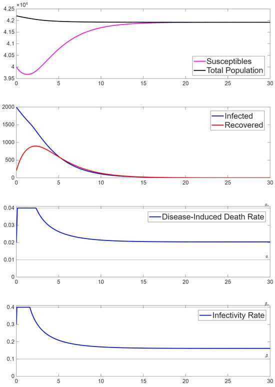
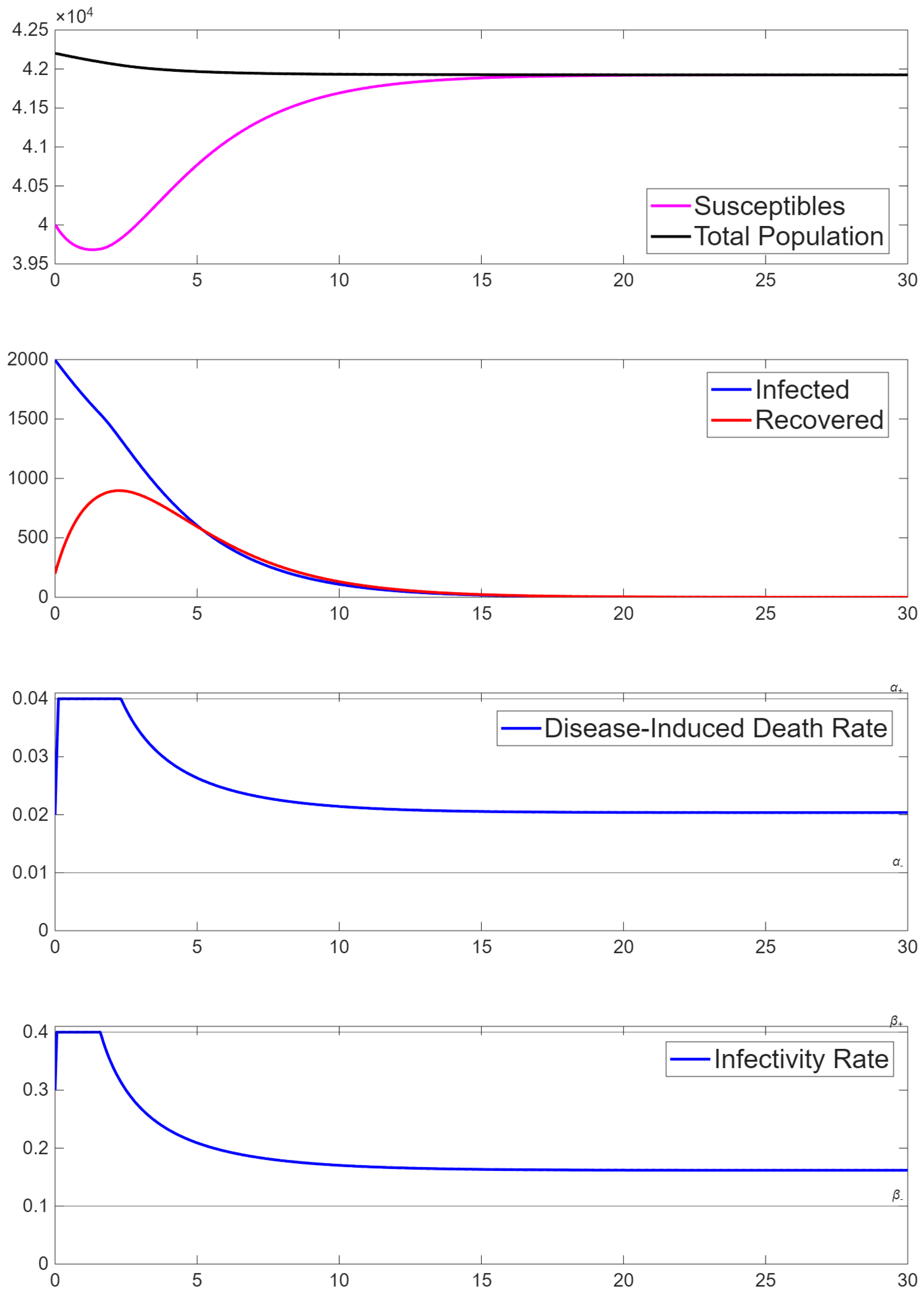
The first example, depicted in Figure 2, begins with $S^0=\mathrm{40,000}$ susceptibles, $I^0=2000$ infected and $R^0=200$ already recovered from the disease. Since the parameters satisfy condition (16), the solution tends to the DFE. The infected and recovered populations decrease to zero after about 20 days, at which point, we have $S=\mathrm{41,926}$ susceptibles making up the total population. We see that the infected population gradually decreases over time, indicating that infected individuals are dying or recovering faster than the rate at which susceptibles are becoming infected. The recovered population increases to almost $R=1000$ before decreasing to zero, showing that most of the previously infected individuals recovered from the disease. The susceptible population takes a small dip, showing that some individuals moved from the susceptible to the infected group before the disease dies off and the populations reach their DFE. In this simulation, the death rate from the disease initially jumps to the upper bound, but after 3 days it decreases until leveling off between the upper and lower bounds. The infectivity rate changes similarly over the same time period. The curves of $\alpha \left(t\right)$ and $\beta \left(t\right)$ are interesting as both rates approach the upper limits quickly and then decrease to their equilibrium values. This shows that in the system both the death rate and the infectivity actually are system-dependent.

Figure 2. Example 1: Convergence to the stable and attracting DFE.

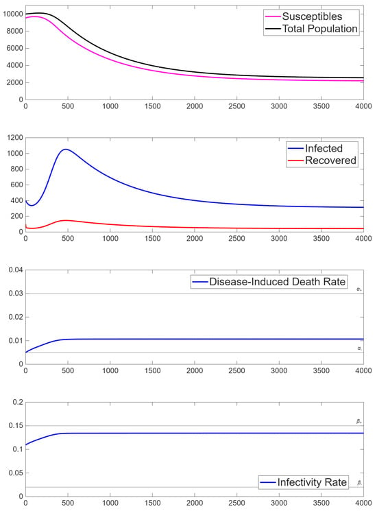
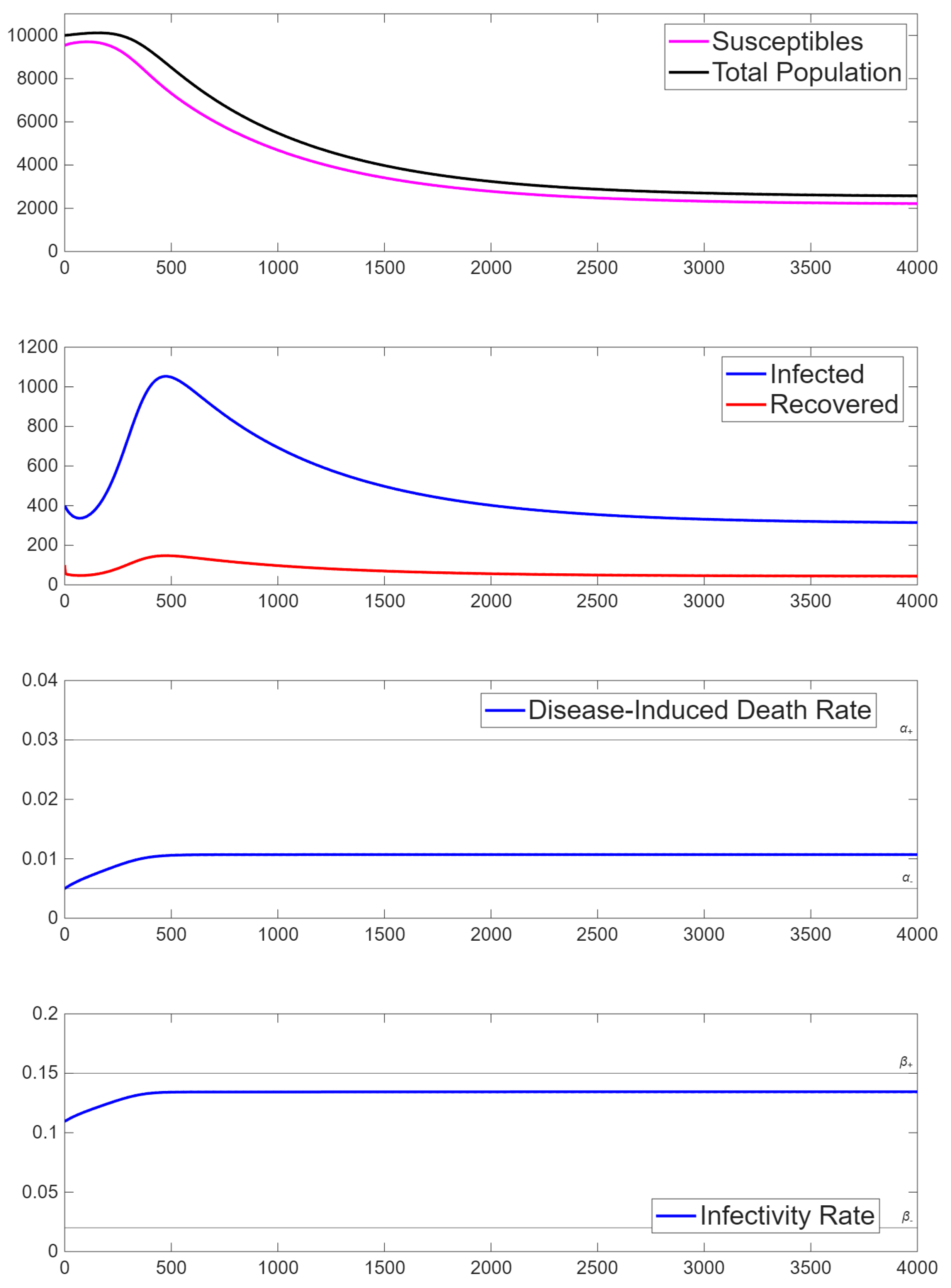
The second simulation outcomes, when the system converges to the EE, are shown in Figure 3.The initial populations are $S^0=9500$ susceptibles, $I^0=400$ infected and $R^0=200$ recovered. Since $\overline{\beta }>(\mu +\overline{\alpha }+\sigma )$, the disease remains in the population as $t\to \infty$. When $0\le t\le 300$, we see that both $\alpha$ and $\beta$ are increasing. This results in a significant decline in the susceptible population and a steep increase in the infected population. When $100\le t\le 500$, the infected and recovered populations increase until they reach their maximum values at around $t=500$. After this time, they decrease to their EE values of $\overline{I}\approx 310$ and $\overline{R}\approx 43$. Both $\alpha$ and $\beta$ reach equilibrium at $t\approx 600$, while the populations $S,I$ and R stabilize when $t\approx 3500$.

Figure 3. Example 2: Convergence to the stable and attracting EE.

6. Numerical Convergence

To obtain confidence in the numerical method, we show the convergence of the algorithm numerically. Since we do not have the exact solution in closed form, we assume that the numerical solution obtained on the finest refinement is the reference ‘exact’ solution. Thus, the exact or reference solution ($\tilde{S},\tilde{I},\tilde{R}$) is the one obtained using Algorithm 1 with $\Delta t={10}^{-6}$. The parameters are as in Table 2. We calculate the numerical solution $u_k$ with $\Delta t={10}^{-k}$, for $k=2,\dots ,5$, and calculate the ${\ell }^{\infty }$ norm of the error up to the final time $T=20$. The rate of convergence is calculated as

$$R_{conv}={\displaystyle \frac{1}{log\left(0.1\right)}}log\left({\displaystyle \frac{\parallel \tilde{u}-u_k{\parallel }_{{\ell }^{\infty }}}{\parallel \tilde{u}-u_{k-1}{\parallel }_{{\ell }^{\infty }}}}\right).$$

The results are presented in Table 3, where we observe that the subsequent numerical solutions converge to the reference solution, and the error decays at a rate of at least 1. This result provides substantial confidence in the numerical method and, therefore, in the numerical solutions.

Table 3. Rates of convergence for the DFE case.

$\mathbf{\Delta }\mathit{t}$	$\parallel \tilde{\mathit{S}}-{\mathit{S}}_{\mathit{k}}{\parallel }_{{\mathit{\ell }}^{\mathit{\infty }}}$	${\mathit{S}}_{\mathbf{rate}}$	$\parallel \tilde{\mathit{I}}-{\mathit{I}}_{\mathit{k}}{\parallel }_{{\mathit{\ell }}^{\mathit{\infty }}}$	${\mathit{I}}_{\mathbf{rate}}$	$\parallel \tilde{\mathit{R}}-{\mathit{R}}_{\mathit{k}}{\parallel }_{{\mathit{\ell }}^{\mathit{\infty }}}$	${\mathit{R}}_{\mathbf{rate}}$
${10}^{-2}$	$9.58$	-	$2.29$	-	$2.58$	-
${10}^{-3}$	$1.41\times {10}^{-1}$	$1.83$	$1.66\times {10}^{-1}$	$1.14$	$5.79\times {10}^{-2}$	$1.65$
${10}^{-4}$	$7.12\times {10}^{-3}$	$1.30$	$8.47\times {10}^{-3}$	$1.29$	$3.15\times {10}^{-3}$	$1.26$
${10}^{-5}$	$2.15\times {10}^{-4}$	$1.52$	$2.60\times {10}^{-4}$	$1.51$	$3.53\times {10}^{-5}$	$1.95$

7. Conclusions

This work describes a new augmented version of the SIR model that mathematically studies the spread of a generic long-term disease. Our SIR-ID model incorporates, in addition, system-dependent variables for the rate of death, $\alpha$, and the rate of infectivity, $\beta$. The motivation behind this model comes from observing the COVID-19 pandemic. As noted in the Introduction, various factors cause changes over time in the death rate and similarly the infectivity rate, such as improved health care, vaccinations and partial immunity to subsequent infections. Also, the limits of the healthcare system to treat infected populations, thus straining hospitals, is another factor.

To make the model applicable to a specific disease, the death and infectivity source functions need be determined from field data. For the model to make epidemiological sense, the differential equations for the death rate ($\tilde{\alpha }$) and the infectivity rate ($\tilde{\beta }$) are incorporated and modified so that they do not fall below or exceed certain ‘realistic’ threshold values.

Following the detailed derivation of the model, we establish the positivity and boundedness of the solutions, which leads to the proof of their existence. This shows that the model makes sense both biologically and mathematically. Then, we study the system’s steady states and show that the DFE is stable and attracting (asymptotically stable) when condition (16) holds. Following the DFE, we study the conditions for the emergence of the endemic equilibrium. Similarly to the DFE, we find the eigenvalues of the Jacobian matrix at the EE when (17) holds. We find that when (16) holds, i.e., ${\mathcal{R}}_0<1$, the DFE is globally asymptotically stable, or stable and attracting. We then show that there is a transcritical bifurcation when ${\mathcal{R}}_0=1$, where the DFE looses its stability and the EE appears and is asymptotically stable, when ${\mathcal{R}}_0>1$. Finally, we state in Theorem 7 that there is no Hopf-type bifurcation and the system does not have oscillatory solutions.

Section 5 presents a simple time-stepping algorithm for the numerical approximations of the solutions. The algorithm has been incorporated in a computer code and two sets of simulations performed. In the first, the system parameters are such that it converges, as $t\to \infty$, to the DFE, showing that in this case, the DFE is stable and attracting (asymptotically stable). In the second simulation, the system parameters are such that it converges to the EE state, since the DFE is unstable. Indeed, the simulations of the model support the DFE and EE, and show how the system approaches them. As noted above, condition (17) guarantees that when the DFE is unstable then in the EE $\overline{I}>0$, and therefore $\overline{R}>0$, too.

We emphasize that in both simulations, the values of $\alpha$ and $\beta$ eventually differ from the constraints, allowing them to be determined by the system. This shows that in these cases imposing their values would lead to different results, which is one of the main motivations of this research.

Now that the basic structure and the behavior of the model have been investigated, there are related issues that warrant further study. Indeed, there is some interest in the study of related extensions of our model, some of which we mention below.

It may be of interest to compare the solutions of our model to solutions of the SIR model in which $\alpha \left(t\right),\beta \left(t\right)$ are given functions, say obtained from curve-fitting experimental data.

One of the main open questions is to model certain disease-informed functional forms of ${\Psi }_{\alpha }$ and ${\Psi }_{\beta }$. This would make it necessary to find the relevant information and see if we can fit the functions to the data. This would make our model applicable to disease-specific results. It seems to us that if for a specific disease one can find an appropriate pair of functions ${\Psi }_{\alpha },{\Psi }_{\beta }$, it may be useful for all applications of the model to this particular disease. This should provide a more accurate predictive tool for those responsible for disease prevention. Moreover, it may be of practical interest to make the recovery rate $\sigma$ a state variable, too.

Since our analysis suggests the possibility of multiple steady-state solutions, the question is of the existence and reachability of such steady states. Reachability refers to the question of given a steady state, how to find the initial conditions that guarantee that the time-dependent solution converges to this steady state as $t\to \infty$. To better understand the model, reachability would be an area of interest.

Another area of interest may be the extension of the model that allows for the sudden appearance of new variants of the disease agents, as was the case with COVID-19. This could be done by introducing randomness to some of the system coefficients.

Furthermore, our model could be used in optimization analysis, leading to applications in vaccination/treatment, general public health or economic studies. Additional simulations are always of interest, together with a comparison to the given information one may have on current diseases.

We note that ways to obtain the system parameters, or find reasonable approximations, are rather complicated, and will be the topics of further research.

Thus, this work is a contribution to the rapidly growing discipline of mathematical epidemiology.

References

- Moore, J.; Shillor, M. A Modified SIR Model with Dependent Infection and Hospitalization Rates. Biomath 2024, 13, 2411146. [Google Scholar] [CrossRef] [Scilit]
- Cesmelioglu, A.; Kuttler, K.L.; Shillor, M.; Spagnuolo, A.M. A Mathematical Model of the COVID-19 Pandemic Dynamics with Dependent Variable Infection Rate: Application to the Republic of Korea. arXiv 2020, arXiv:2008.03248. [Google Scholar]
- Pell, B.; Kalizhanova, A.; Tursynkozha, A.; Dengi, D.; Kashkynbayev, A.; Kuang, Y. Dynamic PD-L1 regulation shapes tumor immune escape and response to immunotherapy. Cancers 2025, 17, 3803. [Google Scholar] [CrossRef] [Scilit] [PubMed]
- Hethcote, H.W. The Mathematics of Infectious Diseases. SIAM Rev. 2000, 42, 599–653. [Google Scholar] [CrossRef] [Scilit]
- Jahedi, S.; Yorke, J.A. When the Best Pandemic Models Are the Simplest. Biology 2020, 9, 353. [Google Scholar] [CrossRef] [Scilit] [PubMed]
- Allen, L.J.S. An Introduction to Mathematical Biology; Pearson: London, UK; Prentice Hall: Saddle River, NJ, USA, 2007. [Google Scholar]
- Wikipedia. Compartmental Models (Epidemiology). Wikipedia, Wikimedia Foundation, 11 May 2025. Available online: https://en.wikipedia.org/wiki/Compartmental_model_(epidemiology) (accessed on 12 June 2026).
- Atherstone, C.J.; Guagliardo, S.A.J.; Hawksworth, A.; O’Laughlin, K.; Wong, K.; Sloan, M.L.; Henao, O.; Rao, C.Y.; McElroy, P.D.; Bennett, S.D. COVID-19 Epidemiology during Delta Variant Dominance Period in 45 High-Income Countries, 2020–2021. Emerg. Infect. Dis. 2023, 29, 1757–1764. [Google Scholar] [CrossRef] [Scilit] [PubMed]
- Coppock, D.; Baram, M.; Chang, A.M.; Henwood, P.; Kubey, A.; Summer, R.; Zurlo, J.; Li, M.; Hess, B. COVID-19 Treatment Combinations and Associations with Mortality in a Large Multi-Site Healthcare System. PLoS ONE 2021, 16, e0252591. [Google Scholar] [CrossRef] [Scilit] [PubMed]
- Liu, J.; Wei, H.; He, D. Differences in Case-Fatality-Rate of Emerging SARS-CoV-2 Variants. Public Health Pract. 2022, 5, 100350. [Google Scholar] [CrossRef] [Scilit] [PubMed]
- Kojima, N.; Klausner, J.D. Protective Immunity after Recovery from SARS-CoV-2 Infection. Lancet Infect. Dis. 2022, 22, 12–14. [Google Scholar] [CrossRef] [Scilit] [PubMed]
- Kloeden, P.; Rasmussen, M. Nonautonomous Dynamical Systems. In Mathematical Surveys; American Mathematical Society: Providence, RI, USA, 2011. [Google Scholar] [CrossRef] [Scilit]
- Allen, L.J.S.; van den Driessche, P. The basic reproduction number in some discrete-time epidemic models. J. Differ. Equ. Appl. 2008, 14, 1127–1147. [Google Scholar] [CrossRef] [Scilit]
- Diekmann, O.; Heesterbeek, J.A.P.; Metz, J.A.J. On the definition and the computation of the basic reproduction ratio R0 in models for infectious diseases in heterogeneous populations. J. Math. Biol. 1990, 28, 365–382. [Google Scholar] [CrossRef] [Scilit] [PubMed]
- Diekmann, O.; Heesterbeek, J.A.P.; Roberts, M.G. The construction of next–generation matrices for compartmental epidemic models. J. R. Soc. Interface 2010, 7, 873–885. [Google Scholar] [CrossRef] [Scilit] [PubMed]
- Ndione, A.B.; Mendy, A.; Onana, C.A. Economic development process: A compartmental analysis of a model with two delays. In Trends in Biomathematics: Chaos and Control in Epidemics, Ecosystems, and Cells; Mondaini, R., Ed.; Springer: Berlin/Heidelberg, Germany, 2021; pp. 355–390. [Google Scholar] [CrossRef] [Scilit]
- Castillo-Chavez, C.; Feng, Z.; Huang, W. On the computation of R0 and its role on global stability. In Mathematical Approaches for Emerging and Reemerging Infectious Diseases: An Introduction; The IMA Volumes in Mathematics and its Applications; Springer: New York, NY, USA, 2002; Volume 125, pp. 229–250. [Google Scholar] [CrossRef] [Scilit]
- van den Driessche, P.; Watmough, J. Reproduction numbers and sub-threshold endemic equilibria for compartmental models of disease transmission. Math. Biosci. 2002, 180, 29–48. [Google Scholar] [CrossRef] [Scilit] [PubMed]
- Castillo-Chavez, C.; Song, B. Dynamical models of tuberculosis and their applications. Math. Biosci. Eng. 2004, 1, 361–404. [Google Scholar] [CrossRef] [Scilit] [PubMed]
Disclaimer/Publisher’s Note: The statements, opinions and data contained in all publications are solely those of the individual author(s) and contributor(s) and not of MDPI and/or the editor(s). MDPI and/or the editor(s) disclaim responsibility for any injury to people or property resulting from any ideas, methods, instructions or products referred to in the content. |
© 2026 by the authors. Licensee MDPI, Basel, Switzerland. This article is an open access article distributed under the terms and conditions of the Creative Commons Attribution (CC BY) license.