


Abstract
This review surveys recent deep learning approaches for solving integral equations, categorizing them into three methodological families: physics-informed embedding, spectral/topological acceleration, and hybrid symbolic–numeric frameworks. The main findings are threefold. First, these methods achieve promising empirical accuracy in oscillatory, high-dimensional, and singular-kernel settings, yet their theoretical foundations remain largely incomplete. Second, from an axiomatic perspective, most approaches lack rigorous guarantees of convergence, stability, and spectral consistency; we formulate five testable propositions that a complete theory should satisfy. Third, we identify five specific unresolved theoretical questions and outline a focused research agenda toward a mathematically rigorous theory of neural operator approximation for integral equations. The novelty of this review lies in its dual computational–axiomatic evaluation and its provision of a structured, problem-oriented framework for future investigations.
Keywords:
integral equations; deep learning; physics-informed neural networks; operator learning; high-dimensional integration; singular kernels MSC:
68T07; 65R20; 45B05; 45D05; 45-02
1. Introduction
Integral equations appear throughout scientific computing as compact formulations of boundary value problems [1,2], inverse problems [3,4], and stochastic processes [5,6]. Classical numerical methods—the Nyström method [7,8,9], the Galerkin method [10,11,12], the collocation method [13,14,15], the method of moments (MoM) [16,17], the boundary element method (BEM) [11,18], and the finite element method (FEM) [19,20]—provide rigorous approximation guarantees for low-dimensional, smooth problems. However, they suffer from well-known limitations when applied to modern challenges: the curse of dimensionality in high-dimensional integration [21,22], numerical instability from singular kernels [23,24,25], and quadratic or higher complexity in dense matrix operations [26,27]. For example, three-dimensional electromagnetic scattering analysis using MoM often encounters memory bottlenecks due to dense matrix storage [28,29]; boundary element methods require intricate regularization for singular integrals [30,31]; and Monte Carlo techniques, while dimension-independent, converge slowly for stochastic integral equations [32,33].
Deep learning has recently been explored as a tool to address these limitations. Neural networks can approximate nonlinear functionals, adapt to data, and be combined with physical constraints through automatic differentiation. This has led to a growing body of work on neural integral equation solvers, ranging from physics-informed neural networks (PINNs) [34] that incorporate integral operators into loss functions to graph neural networks that accelerate electromagnetic scattering computations [29] to sequence-to-sequence models that discover symbolic integration rules [35]. The diversity of approaches, however, makes it difficult to compare methods, understand their relative strengths, and identify open challenges.
Several recent surveys have covered related terrain. Hao et al. [36] and Salvatore et al. [37] reviewed physics-informed machine learning broadly, while Goswami et al. [38] focused on neural operator methods. The seminal DeepONet work [39] established the theoretical foundation for learning solution operators of differential and integral equations, which is highly relevant to our discussion. These works, however, do not specifically target integral equations, nor do they provide a structured comparison of how different neural architectures handle the distinctive difficulties of integral formulations (e.g., singular kernels and global coupling).
This review has two linked objectives. First, it synthesizes recent deep-learning-based methods for solving integral equations through a problem-oriented framework covering oscillatory, high-dimensional, singular-kernel, and coupled-system settings. Second, and more importantly for the present journal, it examines the extent to which these methods admit a coherent axiomatic interpretation. We therefore ask not only which architectures perform well empirically but also which assumptions on operator regularity, kernel smoothness, spectral decay, approximation spaces, and training procedures are required before claims about efficiency, stability, or convergence can be made precise. Under this framing, the review contributes not merely a catalogue of methods, but a mathematically motivated agenda for connecting neural integral solvers with operator theory, approximation theory, and numerical analysis.
The paper is organized as follows. Section 2 presents the mathematical background and an axiomatic perspective. Section 3 describes the literature search and selection criteria. Section 4 details the three methodological families. Section 5 examines how these families address core computational challenges and critically discusses their limitations. Section 7 identifies open problems and emerging research directions. Section 8 concludes. The article is intended for interdisciplinary researchers who seek a structured entry point into the field, as well as for specialists interested in unresolved theoretical and practical issues.
2. Mathematical Foundations and an Axiomatic Perspective
Integral equations can be viewed as operator equations in Banach or Hilbert spaces [11]. Before reviewing deep learning methods, we recall classical mathematical formulations that provide a foundation for understanding neural approximation. This section does not propose new results but establishes notation and highlights axiomatic principles that a rigorous theory of neural integral solvers would need to respect.
2.1. Operator Formulation of Integral Equations
Let X and Y be Banach spaces of functions on a domain . A linear integral equation of the second kind [11] is written as
or in operator form , where is the integral operator with kernel K. Under mild conditions (e.g., ), is compact. The Fredholm alternative then provides a complete characterization of solvability: either is not an eigenvalue of and a unique solution exists for every f, or it is an eigenvalue and solvability requires orthogonality conditions [11].
For nonlinear integral equations (e.g., Urysohn [40] or Hammerstein [41,42]), the operator is nonlinear, but fixed-point theorems [43] (Schauder and Banach) guarantee existence under Lipschitz or compactness assumptions. These classical results are axiomatic in that they rely on abstract properties (compactness, continuity, and contractivity) rather than explicit kernel forms. Any neural solver aiming for provable guarantees must either preserve these properties or work in settings where they are relaxed.
Conventions and notation. Throughout this section, is a bounded domain and unless stated otherwise. The norm denotes the -norm. The symbol N is reserved for the number of degrees of freedom (collocation points, basis functions, or training samples, depending on context); d is the spatial dimension; and m denotes the order of differentiability of the kernel. Asymptotic statements are understood as . For a compact operator, the numerical rank at threshold is the number of singular values larger than . The term “with high probability” refers to the probability taken over the random draw of training data and/or problem instances, as specified in each proposition.
2.2. Axiomatic Requirements for Neural Approximants
A neural network that approximates the solution operator should ideally satisfy: (i) Consistency: As the network capacity (e.g., number of parameters) increases, the approximation error should converge to zero in a suitable norm. (ii) Stability: Small perturbations in the input f or the kernel K should lead to controlled changes in the output (Lipschitz continuity with respect to data). (iii) Spectral correctness: If is self-adjoint and compact, the neural approximation should preserve the sign and decay of its eigenvalues (e.g., a non-negative spectrum for positive-definite kernels).
Classical projection methods (Galerkin and collocation) satisfy these axioms by construction: they project the infinite-dimensional problem onto finite-dimensional subspaces and inherit stability from the well-posedness of the original equation. Neural methods, however, are nonlinear parameterizations and do not automatically inherit these properties. For example, the composition of nonlinear activations may violate compactness, and empirical risk minimization may not enforce spectral constraints.
2.3. Approximation Theory for Neural Operators
The universal approximation theorem [44,45] states that feedforward networks can approximate any continuous function on a compact set arbitrarily well. However, it says nothing about the rate of convergence or about the generalization to families of functions defined by integral equations. For operator learning (mapping functions to functions), a more appropriate framework is the concept of n-widths [46]. A comprehensive theoretical treatment of neural operators, including approximation error bounds and relations to classical numerical analysis, is provided by Kovachki et al. [47]. A concrete realization of neural operator learning is the DeepONet architecture [39], which rigorously proves that neural networks can approximate nonlinear operators to arbitrary accuracy, mirroring the classical universal approximation theorem but for mappings between function spaces. The Kolmogorov n-width of a compact set in a Banach space X is
It quantifies the best possible linear approximation error [48]. Neural networks, being nonlinear approximators, can potentially achieve smaller errors than linear methods for certain function classes (e.g., Barron spaces [49]). For integral equations, the solution set inherits regularity from the kernel. When K is smooth, the solution is smooth, and linear methods (spectral [50] or finite element) are nearly optimal. When K is rough or oscillatory, neural networks may offer advantages, but rigorous upper bounds on for neural approximation of integral operators are largely missing. This is a key axiomatic gap that future research should address.
2.4. Relevance to the Review
The remainder of this review adopts a problem-oriented perspective, categorizing methods by how they handle high frequencies, high dimensions, and singular kernels. The axiomatic viewpoint introduced here serves as a lens for critically assessing the literature: we will ask whether a given method provides convergence guarantees, stability bounds, or spectral consistency. As we shall see, most current approaches are empirical; only a few provide partial theoretical results (e.g., Zappala [51] proves convergence for a spectral neural method under strong smoothness assumptions). The field is far from a complete axiomatic theory, and we highlight this as a major open problem.
2.5. A Propositional Axiomatic Framework for Neural Integral Solvers
General assumptions for the propositions. In the following, we consider a linear integral equation with a compact operator . The neural approximant maps data f to an approximate solution. All propositions are formulated as desiderata for a rigorous theory; they are not claimed as theorems. Unless otherwise specified, limits are taken as the number of degrees of freedom .
Proposition 1 (Operator Class Consistency).
Let be compact and λ not an eigenvalue of . Any neural approximant that claims to solve should satisfy that, for sufficiently large N, the operator is invertible on a subspace of whose dimension is at least the ε-numerical rank with . Moreover, the condition number of on that subspace should remain bounded independently of N.
Proposition 2 (Kernel Regularity Hierarchy).
Assume with . Then a neural solver trained with N samples should achieve a convergence rate
matching the minimax rate for classical linear approximation. If K is weakly singular, i.e., with , the rate should be expressed in terms of α and the regularity of the solution, typically for suitably designed networks.
Proposition 3 (Spectral Decay Preservation).
Let be self-adjoint, compact, and positive definite with eigenvalues satisfying for some . Let be the eigenvalues of the neural approximation , ordered decreasingly. Then for any j up to the numerical rank (with as ), one should have
and the sign pattern must be preserved: for all j. The bound should hold uniformly in j on any compact subset of indices.
Proposition 4 (Stability Under Perturbation).
Let be the neural solution for data f, and the solution when f is perturbed to with . Then the solver should satisfy
where C is independent of θ and δ, and C does not exceed the condition number of by more than a constant factor.
Proposition 5 (Uncertainty Calibration).
Assume the training data consist of i.i.d. draws from a distribution over pairs . For a neural solver that outputs a point prediction and an uncertainty estimate , calibration requires that for any predetermined miscoverage level ,
for almost every , asymptotically as the number of training samples tends to infinity. The probability is taken over the random draw of training data and the random instance f. The constant 2 in the inequality may be replaced by a suitable quantile of the error distribution; the essential requirement is that the predicted intervals achieve the nominal coverage level .
These propositions are deliberately challenging—no existing neural integral solver satisfies all of them. They serve as a benchmark for future theoretical developments and as a checklist for evaluating claims of provable or guaranteed performance in the literature.
Theoretical status of current methods. The gap between these ideal requirements and the current literature is substantial. To date, rigorous convergence and stability guarantees have been obtained only in very restricted settings: for instance, under the strong assumption that the integral kernel is and the network architecture is explicitly aligned with the eigenfunctions of the operator [51]. In general, the following assumptions are necessary for a theoretical guarantee but are seldom verified in practice:
- Compactness and well-posedness: is compact and is not an eigenvalue so that exists and is bounded.
- Kernel regularity: K is sufficiently smooth (e.g., with ) or possesses a low-rank structure, which controls the approximation error.
- Data coverage: The training set is dense enough to capture the relevant function class, and the samples are drawn from the appropriate distribution.
- Optimization convergence: The training algorithm converges to a global minimum of the loss functional, avoiding local minima that do not correspond to accurate solutions.
- Capacity scaling: The network size grows appropriately with the problem dimension and the desired accuracy, without overfitting or underfitting.
Absent these assumptions, the reported performance of neural solvers remains empirical rather than mathematically proven. Consequently, the vast majority of studies reviewed in this article provide only experimental evidence, and the field as a whole still lacks a comprehensive theoretical foundation.
Throughout the remainder of this review, we assess the extent to which current methods approximate these ideal properties, and we identify which propositions remain completely unaddressed by existing work.
3. Survey Methodology
The search and screening process described below was informed by selected elements of the PRISMA 2020 statement [52]; however, this article is a narrative review rather than a formal systematic review, and therefore does not include a PRISMA flow diagram or checklist.
Search strategy. We searched Scopus, Web of Science, IEEE Xplore, and the ACM Digital Library for studies published between January 2019 and May 2026. The search combined the terms “integral equation”, “Fredholm”, “Volterra”, “boundary integral”, “neural network”, “deep learning”, “physics-informed”, “graph neural network”, and “operator learning”. Preprints from arXiv were considered only if they contained unique technical content not yet available in a peer-reviewed venue; such cases are explicitly noted in the text.
Eligibility criteria. Studies were included if they (i) addressed an integral, integro-differential, or stochastic integral equation; (ii) proposed a learning-based solver, acceleration method, or theoretical analysis; and (iii) provided sufficient quantitative or theoretical evidence for comparison. We excluded works focusing solely on differential equations without an integral formulation, papers lacking methodological novelty, and non-archival abstracts.
Screening and data extraction. Two reviewers independently screened titles and abstracts; disagreements were resolved through discussion. Full texts of potentially relevant articles were then examined against the eligibility criteria. From each included study, we extracted information on the proposed method, problem type, reported performance metrics, and theoretical guarantees.
To organize the diverse literature, we adopted a problem-oriented perspective rather than a rigid taxonomy. Specifically, we examined how deep learning methods address three fundamental challenges that limit classical solvers:
- High-frequency oscillations: Solutions that vary rapidly in space or time require methods that avoid spectral bias.
- High-dimensional integration: Exponential growth of cost with dimension demands sub-exponential or linear scaling.
- Singular-kernel resolution: Near-discontinuities or weakly singular kernels cause numerical instability.
Within each challenge, we compared the effectiveness of the three methodological families introduced in Section 4. This perspective allowed a critical appraisal of where each family excels and where it struggles, without imposing a preconceived framework.
All quantitative performance statements (e.g., speedups and error reductions) were taken directly from the original publications, accompanied by their citations. We did not perform independent benchmarking, nor did we average or re-normalize numbers from different sources. When contradictory results existed across studies, we noted them explicitly.
Caveat on quantitative comparisons. All performance figures cited in this review (accuracy, convergence rates, speedups, and memory usage) are reproduced as reported by the original authors and have not been independently verified on a common benchmark. The absence of a standardized evaluation protocol means that direct numerical comparisons across different studies are inherently tentative. Readers should interpret such numbers within the context of the specific test problems, hardware, and implementation details described in the respective publications.
Remark on taxonomy. The three-family taxonomy adopted in this review is based on the dominant computational strategy (physics-informed embedding, spectral/topological acceleration, and hybrid symbolic–numeric frameworks). We recognize that the surveyed methods can also be categorized along other dimensions, including equation type (Fredholm, Volterra, and integro-differential), kernel regularity (smooth, weakly singular, and oscillatory), or neural architecture (MLP, graph neural network, transformer, and operator network). Although a full multidimensional classification is beyond the scope of a single review, the challenge-oriented analysis presented in Section 5 implicitly captures distinctions in kernel properties and equation types, while the architectural choices are highlighted throughout the methodological descriptions. Future systematic reviews may benefit from a formal cross-tabulation of these dimensions.
4. Methodological Taxonomy
Classification criteria and rationale. We define three methodological families according to the dominant computational principle used to handle the integral operator:
- Physics-informed embedding relies on a loss function that directly encodes the integral equation residual, typically via automatic differentiation, and does not require large external training sets.
- Spectral/topological acceleration exploits a transformation of the solution space—such as eigenfunction expansions, Fourier representations, or graph discretizations—to reduce dimensionality or memory footprint.
- Hybrid symbolic–numeric frameworks tightly couple neural networks with symbolic computation, classical iterative solvers, or quantum-inspired components, where the non-neural part is essential to the solver’s functioning.
When a study combines elements from multiple families (e.g., a physics-informed loss with a spectral architecture), we assign it to the family that provides the primary mechanism for solving the integral equation. This taxonomy is deliberately problem-oriented rather than architecture-oriented: it foregrounds the mathematical strategy used to overcome the intrinsic difficulties of integral formulations, thereby helping the reader assess which class of methods is most suitable for a given challenge.
Research on deep learning for integral equations has converged around three methodological families. This section describes each family’s core ideas, representative implementations, and reported performance characteristics as documented in the literature. A critical discussion of limitations follows each subsection.
4.1. Physics-Informed Embedding
Physics-informed neural architectures embed integral operators directly into the network’s loss function or architecture, aiming to enforce physical consistency without requiring large training datasets.
Green’s function embedding. For a linear integral equation with kernel satisfying the Fredholm alternative [53], the Green’s function exists and is unique when is not an eigenvalue of . It satisfies in the distributional sense [11]. Classical results guarantee that G is continuous if K is weakly singular and the domain is sufficiently smooth. Physics-informed neural methods aim to approximate G by minimizing a residual loss; however, they do not explicitly enforce the Fredholm conditions, which may lead to spurious solutions when is near an eigenvalue [54]. The physics-informed iterative neural network encodes Green’s function propagation into network constraints by translating conjugate gradient iterations into parameter updates [28]. For Ku-band antenna design, the authors report 95% accuracy with a fivefold acceleration over traditional solvers [28]. A key advantage is the reduction in training data requirements—approximately 80% less than purely data-driven models. However, the same study notes that accuracy degrades by 25% when applied to millimeter-wave (mmWave) frequencies, indicating sensitivity to the frequency range [55].
Boundary integral networks. The boundary integral neural network (BINN) [30] reduces the problem dimensionality by reformulating partial differential equations as boundary integral equations. For three-dimensional elasticity problems, BINN decreases degrees of freedom by 70% compared to volume discretizations. The authors report relative errors around 0.03 for smooth geometries. Limitations include a 15–20% computational overhead from enforcing boundary constraints and a reported 40% accuracy degradation on fractal boundaries [31].
Geometry-adaptive networks. NURBS-parameterized networks [31] combine geometric transformations with neural approximation, achieving 99% consistency with analytical Laplace equation solutions for crack propagation problems. For isotropic materials, the reported relative error is 0.007. However, when applied to anisotropic composites—which introduce directional dependence—accuracy drops to approximately 70%, illustrating the challenge of generalizing beyond the training geometry distribution.
Critical limitations across physics-informed methods. Despite these advances, physics-informed embedding faces three persistent issues: (i) empirical tuning of loss weights, with no consensus on optimal strategies; (ii) difficulty handling multi-scale features without specialized architectures; and (iii) limited theoretical guarantees of convergence rates. Hybrid approaches that adaptively learn loss weights [56] show promise but remain in early stages.
4.2. Computational Topology Innovation
Spectral and topological methods aim to overcome dimensional and frequency barriers through mathematical transformations of the solution space [50,57].
Spectral neural frameworks. For a compact self-adjoint operator on a Hilbert space, the spectral theorem guarantees the existence of an orthonormal basis of eigenfunctions with eigenvalues such that . The resolvent operator can be expressed via the eigenexpansion, and the solution is . Spectral neural methods [51] aim to learn a finite-rank approximation by truncating this expansion, i.e., replacing by , where and are neural-network-approximated eigenpairs. The approximation error is bounded by the decay rate of the eigenvalues; for smooth kernels, eigenvalues decay exponentially, while for less smooth kernels, only algebraic decay holds. The spectral neural approach [51] maps integral operators to the frequency domain, truncating noise bands while preserving relevant frequencies. The authors prove a theoretical convergence guarantee and demonstrate an order-of-magnitude improvement in interpolation accuracy for oscillatory kernels. Another influential spectral approach is the Fourier neural operator (FNO) [58], which parameterizes the integral kernel in Fourier space and achieves linear complexity for a wide class of PDEs and integral equations. A related method separates electromagnetic field components to capture wavelength-scale features in two-dimensional scattering problems [59].
Graph-based discretizations. GraphSolver [29] represents Rao–Wilton–Glisson (RWG) basis relationships as graph edge weights, enabling memory-efficient electromagnetic scattering analysis. For aircraft-scale targets, the authors report memory usage reduced to 20% of traditional MoM requirements, with a 12-fold speedup. The PhiGRL extension [60] adapts node connectivity for unstructured meshes, demonstrating transfer learning across missile warhead geometries. A limitation noted by the authors is a 220% increase in training time compared to baseline MoM, which may offset runtime gains for one-off simulations.
Tensor decomposition methods. TensorFlow-based residual networks [61] decompose multidimensional kernels into low-rank products, achieving linear complexity scaling for 10-dimensional Fredholm equations. The reported relative error is 0.045 on a benchmark problem, compared to 0.12 for Monte Carlo. Gaussian quadrature acceleration [62] combined with parallel compression triples approximation speeds for Fredholm operators. ReLU-based Monte Carlo sampling [63] controls statistical and approximation errors in Urysohn equations. A common limitation across tensor methods is the need to know or approximate the kernel’s rank structure a priori.
4.3. Hybrid Paradigm Breakthroughs
Hybrid methods combine neural networks with symbolic computation, iterative solvers, or quantum-inspired components to leverage complementary strengths.
Symbolic–numeric fusion. Transformer models have been applied to derive integration rules directly from expressions. As a related advance in symbolic computation [35] applied a sequence-to-sequence model to discover indefinite integrals, achieving 90% accuracy on a held-out test set. Although this work targets symbolic integration rather than the solution of integral equations, it illustrates the potential of neural symbolic methods for integration-related tasks. Another approach [64] uses transformers for symbolic integration, though the authors note that accuracy on unseen expressions remains below 70%.
Quantum-enhanced hybrids. Preliminary explorations have considered quantum computing for high-dimensional integration tasks but to date, no peer-reviewed study has demonstrated a reproducible, asymptotic quantum advantage for solving integral equations. Claims of quantum-inspired acceleration should be interpreted as referring to classical algorithms that borrow concepts from quantum information, not to genuine quantum hardware implementations with proven speedups. Readers are cautioned against extrapolating early proof-of-concept results to practical-scale problems.
Iterative neural networks. The physics-informed iterative neural network [28] transforms conjugate gradient mechanics into parameter updates, accelerating combined field integral equation (CFIE) solutions by a factor of five as reported. Gated recurrent unit (GRU) networks [65] convert integral equations into sequential tasks via Monte Carlo discretization, stabilizing convergence for Fredholm equations. Reinforcement learning frameworks [66] optimize light transport integrals through dynamic sample generation, improving rendering efficiency by 50% via policy-guided loss design. A common criticism is that these hybrid models introduce additional hyperparameters (e.g., the number of inner iterations and the learning rate for the symbolic component) with no established tuning guidelines.
4.4. Summary of Methodological Families
Table 1 summarizes the reported strengths and limitations of each family based on the literature surveyed. No single family dominates across all problem types; the choice of method depends on the specific computational challenge, as will be analyzed in Section 5.
Table 1.
Comparative summary of methodological families based on literature reports.
Beyond the application-specific strengths and limitations summarized above, a deeper analytical comparison requires examining how each family performs along five fundamental dimensions that are central to the axiomatic perspective introduced in Section 2: the class of operators they can handle, the required regularity of the integral kernel, their computational complexity, the nature and strength of convergence evidence, and whether they provide uncertainty quantification. Table 2 organizes the three methodological families along these dimensions based on the available literature.
Table 2.
Systematic comparison of methodological families across five analytical dimensions.
As Table 2 illustrates, no methodological family excels across all five dimensions. Physics-informed embedding methods are the most broadly applicable in terms of operator class and kernel regularity but offer the weakest theoretical convergence guarantees and essentially no uncertainty quantification. Spectral and topological methods provide stronger theoretical foundations—including proven exponential convergence for analytic kernels—but are restricted to compact self-adjoint operators and smooth kernels. Hybrid methods promise the greatest flexibility and potentially favorable complexity, yet they currently lack any convergence proofs and introduce additional sources of uncertainty (e.g., from quantum components). This systematic comparison reinforces the central argument of this review: the field is computationally promising but remains mathematically under-founded, particularly in terms of convergence guarantees and uncertainty quantification.
5. Addressing Core Challenges: A Critical Appraisal
Classical integral equation solvers struggle with three fundamental challenges: high-frequency oscillations, high-dimensional integration, and singular-kernel resolution. This section examines how the methodological families described in Section 4 address each challenge, based on evidence reported in the literature. Rather than presenting new benchmark results, we critically compare reported findings, highlight contradictions where they exist, and identify unresolved issues.
5.1. High-Frequency Oscillations
Solutions to integral equations that oscillate rapidly in space or time pose a well-known difficulty for standard neural networks due to spectral bias, i.e., the tendency to learn low-frequency components first. Several specialized architectures have been proposed to mitigate this issue.
High-frequency oscillations correspond to solutions whose Fourier transform is supported on high wavenumbers. For an integral operator with a kernel that is not smoothing (e.g., the identity operator or a singular kernel), the solution u may contain frequency components up to the Nyquist limit of the discretization. The Nyquist–Shannon sampling theorem states that to resolve a frequency , one needs at least samples per dimension [68]. For integral equations in d dimensions, this leads to a sample complexity of , which is the root of the curse of dimensionality for oscillatory problems. Neural methods try to bypass this via spectral bias: networks learn low frequencies first [69], requiring specialized architectures (Fourier features, multi-scale) to represent high frequencies. However, no known neural architecture can achieve sub-exponential scaling in without exploiting additional smoothness or sparsity.
Multi-scale PINNs [70] embed spatial features at multiple resolutions using Fourier feature mappings. For scattering problems in the 1–10 GHz range, the authors report a normalized mean absolute error (MAE) of 0.018, compared to 0.035 for standard PINNs and 0.021 for MoM. In the 10–100 GHz range, the reported MAE for multi-scale PINNs increases to 0.067, while MoM reaches 0.153. Above 100 GHz, multi-scale PINNs achieve 0.159 versus MoM’s 0.412. The authors attribute the improvement to frequency decomposition, though they note that performance degrades when the frequency content spans more than three decades.
An alternative spectral-graph neural network [51] operates directly in the frequency domain by truncating noise bands. For the same test problems, the authors report MAEs of 0.015 (1–10 GHz), 0.042 (10–100 GHz), and 0.098 (>100 GHz). The frequency-domain approach appears to maintain lower error at high frequencies than multi-scale spatial methods, but the two studies use different test geometries, making direct comparison tentative.
A common limitation across both approaches is the lack of theoretical guidance on how to choose the number of frequency bands or the truncation threshold. Additionally, reported performance often depends on the specific test geometry; results on spheres may not generalize to sharp-edged objects. No study to date has systematically compared these methods on a common benchmark suite, so claims of superiority should be treated as preliminary. A practical open question is whether multi-scale methods can be combined with spectral truncation to further improve performance.
5.2. High-Dimensional Integration
The exponential growth of computational cost with dimension—the curse of dimensionality—limits classical quadrature and Monte Carlo methods for integral equations in dimensions beyond five or six. Neural methods aim to exploit low-rank structures or adaptively sample the domain.
The curse of dimensionality for multivariate integration can be quantified by the worst-case error of quadrature rules. For a function of d variables with bounded mixed derivative (Sobolev space ), the optimal convergence rate is for deterministic methods and for Monte Carlo. Classical results [71] show that no deterministic method can achieve a rate better than , which is exponentially slow in d. However, if the function has additional structure—such as low effective dimension, additivity, or a sparse Fourier representation—methods like sparse grids, tensor trains, or neural networks can break this barrier. The success of tensor decomposition and Legendre networks for integral equations relies on the assumption that the integral kernel has low-rank structure in the sense of the singular value decomposition, i.e., with r small. This is an axiom that must be verified for the problem at hand.
Tensor decomposition methods [61] represent multidimensional kernels as low-rank products. For a 10-dimensional Fredholm equation of the second kind, the authors report a relative error of 0.045 with linear complexity scaling, compared to 0.12 for Monte Carlo. The memory footprint is reported as 4.8 GB for the neural method versus 2.1 GB for Monte Carlo, indicating a trade-off between accuracy and memory.
A tensor-WENO (weighted essentially non-oscillatory) scheme [62] combining quadrature acceleration with tensor compression achieves a relative error of 0.0003 on an eight-dimensional problem while using only 0.7 GB of memory. However, the authors note that the method requires the kernel to have a low-rank structure, which is not guaranteed for many practical problems.
Legendre polynomial networks [32] exploit basis orthogonality to achieve reported errors as low as 0.00001 on 12-dimensional financial path integral problems. The same study reports a 70% faster convergence compared to Monte Carlo. A limitation is that the Legendre basis must be truncated at a degree that grows with dimension, leading to an exponential increase in the number of basis functions unless the solution is very smooth.
A recurring theme is that each method exploits a specific structural property (low-rank, smoothness, orthogonality) that may not hold for arbitrary integral equations. There is no general-purpose high-dimensional neural solver. Furthermore, most reported results are for synthetic test problems; applications to real-world high-dimensional problems (e.g., uncertainty quantification in 20+ parameters) remain scarce. The community would benefit from a standardized set of high-dimensional test problems with varying degrees of kernel complexity.
5.3. Singular-Kernel Resolution
Singular kernels (e.g., in electrostatic or elastic problems) cause numerical instability and require careful regularization. Neural methods have approached this challenge through geometry-aware architectures and dimension reduction.
Singular kernels of the form for give rise to integral operators that are not compact on but are bounded from to if . For example, the Newtonian potential in 3D has , which is less than , so the operator is compact on . However, the kernel is not integrable in the usual sense, and the integral must be interpreted as a principal value or as a weakly singular integral. The classical theory of singular integrals (Calderón–Zygmund [72,73]) shows that these operators are bounded on spaces and satisfy a Hormander condition [74]. The challenge for numerical methods is to evaluate the integral near the singularity without loss of accuracy. Geometry-adaptive methods (NURBS) essentially perform an analytic regularization by mapping the singularity to a coordinate line, which is a technique rooted in the method of stationary phase and resolution of singularities [75]. Neural methods that ignore the singularity often produce large errors unless they incorporate these analytic transformations.
The boundary integral neural network (BINN) [30] reduces the problem to boundary integrals, avoiding volume singularities. For three-dimensional elasticity with a smooth boundary, the authors report a relative error of 0.03 and a reduction in degrees of freedom by 70% compared to FEM. Convergence is reported as , where N is the number of boundary collocation points.
NURBS-parameterized attention networks [31] combine geometric transformations with self-attention to localize singular behavior around crack tips. For isotropic materials, the reported relative error is 0.007 with a convergence rate of . For anisotropic composites, the error increases to approximately 0.30, indicating strong dependence on material symmetry.
A residual integral solver network (RISN) [76] integrates Gaussian quadrature with fractional derivative terms, achieving a relative error of 0.015 for fractional integro-differential equations with weakly singular kernels. Convergence is reported as .
Geometry-adaptive methods (NURBS-based) excel when the singularity location is known a priori (e.g., crack tips). For problems with moving or unknown singularities (e.g., contact mechanics), the advantage diminishes. Attention-based methods offer flexibility but require more training data. A fundamental limitation across all methods is the lack of rigorous error bounds for singular kernels; current results are empirical. Moreover, the reported convergence rates come from different test problems and are not directly comparable.
5.4. Hybrid and Coupled Systems
Many real-world problems involve integral equations coupled with differential or algebraic equations. Hybrid solvers address such multiphysics systems.
Coupled systems of integral, differential, and algebraic equations arise from multiphysics models (e.g., fluid–structure interaction). The mathematical well-posedness is often established via semigroup theory or monotone operator theory. A common technique is to rewrite the system as a single integral equation of the second kind on a product space, but this leads to a larger kernel matrix. The convergence of iterative splitting schemes (e.g., waveform relaxation) is governed by the spectral radius of a certain integral operator. Neural hybrid methods essentially learn the splitting operator or the coupling terms from data. From an axiomatic viewpoint, a rigorous analysis would require verifying that the learned coupling preserves contractivity or dissipativity properties of the original system. Most current neural hybrid solvers do not provide such verification.
A transformed field expansion method [77] for Fredholm–ODE coupling reports a relative error of 0.04 with convergence . An attention-based Navier–Stokes integrator (ANIE) [78] achieves a relative error of 0.07 for coupled integral–differential formulations, with a convergence rate of . The authors note that training time is approximately 3.5 times higher than a baseline without attention.
Legendre–Gauss methods [79] for Volterra–Fredholm–Hammerstein systems achieve the fastest reported convergence rate () by decoupling time and space. A PINN-based integral approach for capacitance extraction [80] reports a relative error of 0.01.
Hybrid methods often improve convergence at the cost of increased training complexity. The choice between spectral–temporal decoupling (Legendre–Gauss [79]) and attention-based coupling (ANIE) depends on whether the problem is dominated by smooth temporal dynamics or by long-range spatial interactions. No unified framework exists for selecting the appropriate hybrid architecture given problem characteristics.
5.5. Summary of Challenge-Specific Insights
Table 3 synthesizes the reported performance and limitations for each challenge based on the literature. Several cross-cutting observations emerge:
Table 3.
Summary of reported performance by challenge. Errors are normalized mean absolute errors or relative errors as reported in the original studies; ranges reflect different test problems or frequency bands.
- No single method dominates all challenges. Spectral methods perform well for high frequencies; tensor methods excel at high dimensions; geometry-adaptive methods are best for known singularities.
- Direct comparisons across studies are hindered by different test problems, metrics, and hardware. The field lacks a common benchmark suite.
- Many reported performance numbers come from single studies and have not been independently replicated.
- Theoretical understanding—particularly error bounds and convergence guarantees—lags behind empirical demonstrations.
These observations motivate the open problems discussed in Section 7.
5.6. Computational Scalability
While many neural operator methods claim strong performance in high-dimensional settings, published studies often lack a systematic account of computational resources. Based on the literature reviewed, we observe the following trends and gaps:
- Asymptotic complexity. Physics-informed methods typically scale as to due to dense quadrature, while spectral and tensor-based methods can achieve or near-linear scaling under low-rank assumptions. However, the constant factors are rarely reported.
- Memory footprint. Graph-based and tensor decomposition methods (e.g., GraphSolver [29] and Legendre networks [32]) report significant memory reductions relative to traditional solvers, but comparisons are often made against unoptimized baselines.
- Training time and GPU requirements. Few studies provide detailed information on GPU hardware, wall-clock training time, or energy consumption. For instance, ref. [29] notes a 220% increase in training time compared to MoM, yet GPU specifications are not disclosed. The lack of standardized reporting impedes fair comparison and practical deployment.
- Large-scale viability. To date, most neural integral solvers have been tested on problems of moderate size (up to degrees of freedom). Extrapolation to industrial-scale applications remains unverified.
We encourage future studies to report these practical metrics alongside accuracy so that researchers can better assess suitability for large-scale applications.
6. Illustrative Case Studies from the Literature
To illustrate how different deep learning methods perform in specific application domains, this section presents four representative case studies drawn from the literature. Each case highlights the method’s reported strengths, its documented limitations, and the underlying mathematical principles that explain the method’s behavior. The selection spans electromagnetic computation, mechanical analysis, financial engineering, and computational physics.
6.1. Electromagnetic Scattering: Graph-Based Acceleration
Electromagnetic scattering analysis for electrically large targets is a classical application of integral equations, typically solved via the method of moments (MoM). The computational bottleneck is the dense impedance matrix, which scales as in memory and in time for direct solvers.
GraphSolver [29] represents Rao–Wilton–Glisson (RWG) basis functions as nodes in a graph, with edge weights encoding electromagnetic interactions. The integral operator is thereby approximated by graph convolutions, enabling sparse representations.
The MoM impedance matrix Z has entries , where is the Green’s function of the Helmholtz equation. For a basis with local support, Z is not sparse but can be approximated by a sparse matrix after a suitable transformation. GraphSolver treats the sparsity pattern as the adjacency of a graph that approximates the geometry. This is analogous to the fast multipole method (FMM) [81,82] or -matrix compression, both of which exploit low-rank properties of K for well-separated groups of basis functions. The graph approach replaces analytic low-rank approximations (e.g., multipole expansions) with a learning-based adjacency, which may capture non-standard geometries but lacks a priori error bounds.
For aircraft-scale targets, the authors report significant acceleration and memory reduction compared to conventional MoM, with a trade-off in increased training time. The method also demonstrates transfer learning across similar geometries using PhiGRL [60]. However, the accuracy degrades for non-convex or multi-scale features, a common challenge for graph-based discretizations. The authors note that the method is best suited for repeated simulations on similar geometries, where the training cost can be amortized. A quantitative comparison of the computational performance between GraphSolver and conventional MoM is shown in Figure 1.
Figure 1.
Electromagnetic scattering analysis: comparison of MoM and GraphSolver. GraphSolver achieves a reported speedup and memory reduction by approximating the dense impedance matrix with a sparse graph convolution. The underlying principle is the low-rank compressibility of the Green’s function at high frequencies, which the graph learning tries to discover automatically.
6.2. Mechanical Analysis: NURBS-Parameterized Networks for Crack Propagation
Fracture mechanics problems involve singular stress fields at crack tips, which require high resolution and careful regularization in traditional finite element methods.
NURBS-parameterized networks [31] combine geometric transformations with self-attention mechanisms to localize the singular behavior around crack tips. The integral equation formulation of the elasticity problem is solved by a neural network whose inputs are NURBS coordinates.
The stress field near a crack tip behaves as , where r is the distance from the tip. This singularity is not smooth, and standard polynomial bases converge slowly. In the boundary element method, one typically enriches the basis with asymptotic crack-tip functions. NURBS (Non-Uniform Rational B-Splines) provide a way to map the physical domain with a crack to a parameter domain where the singularity becomes a coordinate line. The neural network then approximates a smooth function in the parameter domain. This is equivalent to an analytic preconditioner: the network learns a representation that factors out the singularity so that the remaining function is smooth and can be learned efficiently. The self-attention mechanism further localizes the receptive field to the crack-tip region, mimicking the idea of adaptive mesh refinement.
For isotropic materials with a known crack geometry, the method achieves very high accuracy (relative error below 0.01) and a fast convergence rate. When applied to anisotropic composites, the accuracy drops significantly (to around 70%), because the angular dependence of the singularity changes and the fixed NURBS parameterization no longer aligns with the true asymptotic expansion. The method requires a priori knowledge of crack location, limiting its use in propagation simulations. Figure 2 illustrates the performance gap between isotropic and anisotropic materials for crack-tip stress prediction.
Figure 2.
Crack-tip stress prediction error: NURBS-parameterized networks achieve high accuracy for isotropic materials by mapping the singularity to a smooth coordinate. The degradation for anisotropic materials illustrates the importance of matching the parameterization to the true asymptotic structure.
6.3. Financial Engineering: Legendre Polynomial Networks for Derivative Pricing
Option pricing under stochastic volatility models leads to high-dimensional integral equations (e.g., the Fredholm equation for American options). Traditional methods include Monte Carlo simulation and finite difference methods, both of which face the curse of dimensionality.
Legendre polynomial networks [32] exploit the orthogonality of Legendre basis functions to approximate the integral kernel. The network’s architecture is designed to match the spectral properties of the pricing operator, enabling linear complexity scaling with dimension.
For a problem of dimension d, a straightforward tensor-product basis would have terms, which is exponential. However, if the kernel is of the form with small rank r, the solution can be represented in a separable form. The Legendre expansion is particularly efficient for functions on hypercubes because the basis is orthogonal and the coefficients decay rapidly for smooth functions. For pricing problems, the payoff function (e.g., max of assets) is not smooth, but the expectation operator (the integral kernel) smooths it out, leading to a solution with bounded mixed derivatives. The Legendre network learns the expansion coefficients for each dimension independently but with a low-rank coupling across dimensions, which is essentially a tensor decomposition. The near-linear scaling in d is achieved because the rank r is independent of d for many financial models (e.g., independent assets).
The method achieves very low relative errors (on the order of ) for smooth payoffs and dimensions up to 12, with reported faster convergence compared to Monte Carlo. For non-smooth payoffs (e.g., digital options), the required degree of Legendre polynomials increases, reducing efficiency. The method also assumes the kernel has a low-rank structure, which may not hold for strongly correlated assets or jump-diffusion models. Figure 3 compares the computational time of the Legendre network and Monte Carlo as a function of the number of dimensions, demonstrating the near-linear scaling of the Legendre approach.
Figure 3.
High-dimensional integration efficiency (Section 5.3). The plot shows the computational time (in seconds) versus the number of dimensions for an option pricing problem with dimensions ranging from 5 to 50. The Monte Carlo method (blue) exhibits linear growth with a steeper slope, while the Legendre polynomial network [32] (red) achieves near-linear scaling with a significantly lower growth rate. This demonstrates the computational advantage of exploiting the low-rank structure of the integral kernel for high-dimensional problems.
6.4. Computational Physics: Fourier-Integral Operators for Thermal Conductivity
Predicting thermal conductivity in functionally graded materials requires solving integral equations with multi-scale coefficients. Traditional finite element methods require fine meshes to resolve material gradients, leading to high computational cost.
Fourier-integral neural operators (FIE-NO) [83] embed spectral features into the network architecture, encoding the integral kernel in the Fourier domain. This allows the network to capture both slow and fast variations in material properties.
The integral operator for thermal conductivity can be expressed as a pseudo-differential operator with symbol . In the Fourier domain, applying the operator corresponds to multiplication by followed by an inverse Fourier transform. When the material is graded slowly, the symbol is smooth in and can be approximated by a low-order polynomial, leading to a sparse representation in physical space. The Fourier-integral neural operator learns a parameterization of the symbol from data, effectively performing a learned sparse transform. This is analogous to the method of the Fourier neural operator (FNO) but adapted to the specific kernel structure of the thermal conductivity problem. The advantage is that the complexity remains linear in the number of spatial points because the Fourier transform is fast (FFT). However, the method inherits the limitations of FFT-based methods: it requires periodic or extended boundary conditions and may suffer from Gibbs phenomena for non-smooth material profiles.
For graded thermal conductivity problems, FIE-NO achieves low relative errors (below 2%) across a range of material profiles, outperforming FEM. The method maintains linear complexity with respect to the number of spatial points. Limitations include the requirement for periodic or extended boundary conditions and sensitivity to the number of Fourier modes retained. The dependence of the relative error on the number of retained Fourier modes is shown in Figure 4.
Figure 4.
Thermal conductivity prediction (Section 5.4). Relative error of the Fourier-integral neural operator (FIE-NO) [83] compared with a finite element reference solution, as a function of the number of retained Fourier modes. The FIE-NO maintains an error below 2% across a range of graded material profiles by learning the spectral representation of the integral kernel. The method is most effective when the material properties are smooth and periodic boundary conditions apply.
6.5. Cross-Cutting Observations: Mathematical Generalizability
The four case studies reveal several recurring mathematical themes:
- Singularity preconditioning: Methods that explicitly factor out known singularities (NURBS) or incorporate asymptotic expansions (Legendre) achieve high accuracy but lack flexibility. From an axiomatic viewpoint, they correspond to a priori knowledge of the solution’s analytic structure.
- Sparsity and low-rank structure: Both graph-based and Fourier methods exploit the fact that the integral kernel, while dense, can be approximated by a low-rank operator after a suitable transformation (graph adjacency or Fourier truncation). This is the same mathematical principle underlying the fast multipole method and -matrices.
- Dimension dependence: The Legendre network’s success in high dimensions relies on the existence of a low-rank separated representation of the kernel. It is not a universal remedy; for kernels without this property, the method’s complexity reverts to exponential.
- Lack of universal architecture: No single method outperforms others across all problem types. This is consistent with the no free lunch theorems for approximation: the optimal approximant depends on the function class, and there is no universal neural network that is optimal for all integral operators.
These observations lead to a fundamental question: Does there exist a neural architecture that is universally optimal for a broad class of integral operators? The answer likely requires combining multiple building blocks (spectral, graph, attention) in a problem-adaptive way. This is analogous to the concept of adaptive approximation in classical approximation theory, where the convergence rate depends on the Besov smoothness of the target function. For integral equations, an analogous smoothness class could be defined by the decay of singular values of the solution operator. Developing a theory that characterizes these classes and provides architectural guidelines is a major open problem, which we discuss further in Section 7.
7. Emerging Directions and Open Problems
The literature reviewed in Section 4, Section 5 and Section 6 reveals both progress and persistent gaps. This section identifies several emerging research directions that, in our view, merit attention from the community. Rather than presenting solutions, we highlight open problems and potential pathways, with the aim of stimulating further investigation.
7.1. Quantum-Classical Hybrid Architectures
Early exploratory studies have investigated quantum annealing for high-dimensional integral equations [67]. On small-scale synthetic instances (up to 10 dimensions) using specialized hardware, the authors report a reduction in time-to-solution relative to a classical baseline. However, these results have not been independently replicated, the problem sizes remain far below those of practical interest, and no asymptotic advantage has been established. Several critical open problems must be addressed before quantum or quantum-inspired methods can be considered viable for integral equation solving:
Open problems. (i) Can quantum amplitude amplification be used to accelerate Monte Carlo sampling for stochastic integral equations, and under what conditions would this yield a provable (rather than empirical) advantage? (ii) What classes of integral kernels admit natural sparse representations in quantum computational bases, and how does the encoding cost scale with problem size? (iii) How can error mitigation techniques (e.g., zero-noise extrapolation and probabilistic error cancellation) be adapted to integral equation solvers, and what are the resulting overheads? (iv) What constitutes a fair classical baseline for comparison (e.g., optimized tensor train methods and fast multipole methods) when evaluating quantum approaches?
7.2. Dynamic Operator Adaptation via Meta-Learning
Current neural integral solvers are typically trained once for a fixed equation family. For inverse problems or parametric studies where the integral operator changes (e.g., varying kernel function, boundary conditions, or material parameters), retraining from scratch is inefficient.
Potential approaches. Meta-learning frameworks (e.g., MAML [84] and Reptile [85]) have been applied to ordinary and partial differential equations, but their use for integral equations is unexplored. One could envision a meta-trained model that adapts to new kernel functions with few gradient steps. A key challenge is avoiding catastrophic forgetting when the operator family is diverse.
Open questions. (i) What is an appropriate meta-distribution over integral operators (e.g., kernels with varying smoothness, singularity strength, or oscillatory frequency)? (ii) How can meta-learning be combined with physics-informed losses to preserve constraint satisfaction after adaptation?
7.3. Hardware-Aware Algorithm Co-Design
Deploying neural integral solvers on edge devices or in real-time simulation pipelines requires attention to hardware constraints (memory, energy, latency). Sparse tensor cores, near-memory computing, and analog in-memory computing offer potential, but existing work has not systematically optimized integral-equation-specific kernels (e.g., singular quadrature and convolution with Green’s functions) for these accelerators. A recent effort in this direction is the parallel training framework proposed by Ren et al. [86], which demonstrates near-linear scaling on multi-GPU systems for solving large-scale integral equations, highlighting the importance of co-design between neural architectures and distributed computing infrastructure.
Opportunities. (i) Designing network architectures whose computational patterns match tensor core capabilities (e.g., block-sparse matrix multiplications). (ii) Exploiting the low-rank structure of many integral kernels to reduce memory movement. (iii) Developing mixed-precision training schemes that maintain accuracy for singular integrals.
Barriers. Lack of standardized benchmarks for hardware-aware comparison, proprietary hardware details, and the need for cross-disciplinary collaboration between numerical analysts and computer architects.
7.4. Theoretically Grounded Uncertainty Quantification
Most neural solvers output point estimates without uncertainty intervals. For safety-critical applications (e.g., aircraft scattering, crack propagation, and medical imaging), calibrated uncertainty is essential. Bayesian neural networks, deep ensembles, and conformal prediction offer possible routes, but they must preserve physical constraints.
Open challenges. (i) How to propagate uncertainty through integral operators (e.g., via Monte Carlo dropout in the spectral domain)? (ii) Can we derive error bounds that are both tight and computationally tractable for neural approximations of compact operators? (iii) What is the correct probabilistic interpretation of physics-informed losses?
7.5. Explainability and Physics Consistency Verification
Attention maps have been shown to correlate with vortex structures in fluid dynamics simulations [78], but a general framework for verifying that a neural solver respects integral equation properties (e.g., compactness of the operator, coercivity, and spectral properties) is missing.
Possible directions. (i) Adapting automated theorem proving or symbolic differentiation to generate human-readable certificates of physical consistency. (ii) Developing saliency methods specifically for integral operators (e.g., visualizing which regions of the integration domain contribute most to the solution). (iii) Using Lipschitz constants or spectral norms to bound approximation errors.
7.6. Standardized Benchmarks and Reproducible Leaderboards
A recurring theme in this review is the difficulty of comparing methods across studies due to different test problems, metrics, hardware, and implementation details. The field would benefit from a community-driven benchmark suite for integral equation solving, analogous to existing benchmarks for PDEs (e.g., PINN benchmarks and neural operator benchmarks).
Desirable features of a benchmark suite. (i) Canonical problems across 1D–10D, Fredholm/Volterra, singular/non-singular, with varying kernel types. (ii) Standardized metrics: relative error (, ), computation time, memory usage, training epochs, and energy consumption. (iii) Multiple hardware configurations (CPU, GPU, and TPU) to assess portability. (iv) Baseline implementations (MoM, BEM, Monte Carlo) for comparison.
Community efforts. A few initial steps have been taken (e.g., the DeepXDE library includes some integral equation examples), but a systematic, peer-reviewed benchmark is yet to emerge. Organizing a challenge or competition at a conference (e.g., NeurIPS, ICLR, and ICML) could accelerate progress.
7.7. Reproducibility and Open Science
Reproducibility is increasingly recognized as a cornerstone of scientific machine learning. However, the literature on neural integral equation solvers remains fragmented in this respect. We highlight the following resources and gaps:
Publicly available datasets. At present, no large-scale, curated dataset specifically designed for benchmarking integral equation solvers exists. Most studies generate synthetic data using predefined kernels and random right-hand sides. Exceptions include the collection of boundary integral examples distributed with DeepXDE [87] and a few financial pricing datasets used in Legendre network studies [32]. The creation of a community repository covering Fredholm, Volterra, and integro-differential problems with varying regularity would be a significant contribution.
Open-source implementations. Several open-source libraries offer partial support for integral equations. DeepXDE [87] provides a physics-informed framework that can handle integral terms through custom loss functions. NeuralOperator [58] implements Fourier Neural Operators and can be adapted to integral formulations. GraphSolver [29] and the Legendre network code from [32] are available upon request. However, a unified, modular toolkit that supports multiple neural architectures and standardized evaluation protocols is still lacking.
Recommendations for community-wide initiatives.
- Establish a curated benchmark suite with canonical problems in 1–10 dimensions, including singular, oscillatory, and coupled systems, with reference solutions computed to high accuracy.
- Define standardized reporting metrics: relative and errors, wall-clock time, peak memory usage, GPU model, and number of trainable parameters.
- Organize a recurring challenge (e.g., at NeurIPS or ICLR) to track progress and foster reproducible research.
- Encourage all authors to release code, trained models, and data alongside publications, ideally with a DOI via Zenodo or similar.
Such efforts would considerably accelerate progress and improve the reliability of published results in this emerging field.
7.8. Summary of Open Problems
Table 4 summarizes the six directions and their key open questions. Addressing these problems will require collaboration between numerical analysts, machine learning researchers, and domain scientists. While the potential payoff is high—enabling solutions to previously intractable integral equations—the path forward is likely to involve incremental progress on multiple fronts.
Table 4.
Summary of emerging directions and their associated open problems.
8. Conclusions
This review has surveyed the rapidly growing literature on deep-learning-based integral equation solvers, organizing it into three methodological families through a problem-oriented lens. Unlike previous surveys of physics-informed machine learning or neural operators, the present work is distinguished by its exclusive focus on integral formulations and by its systematic evaluation from both computational and axiomatic standpoints.
This review shows that deep learning has opened a promising but still theoretically fragmented pathway for solving integral equations. The literature demonstrates encouraging empirical progress in oscillatory, high-dimensional, and singular-kernel settings, yet the supporting mathematical theory remains uneven and often problem-specific.
The novelty of this review is threefold. First, we provide a structured taxonomy—physics-informed embedding, spectral/topological acceleration, and hybrid symbolic–numeric frameworks—that foregrounds the mathematical strategy employed by each method rather than its architectural details. Second, we formulate five explicitly testable propositions (operator consistency, kernel regularity hierarchy, spectral decay preservation, stability under perturbation, and uncertainty calibration) that constitute a minimal axiomatic framework for a rigorous theory of neural integral solvers. These propositions serve as both a diagnostic tool for evaluating existing methods and a roadmap for future theoretical developments. Third, we identify five specific unresolved theoretical questions and propose concrete community-level actions—including a standardized benchmark suite and open-science practices—that would accelerate progress toward a mathematically coherent discipline.
From an axiomatic perspective, the central message is not simply that neural solvers can work but that the field now requires a clearer axiomatic and operator-theoretic foundation. In particular, future work should characterize admissible operator classes, identify appropriate function spaces for neural approximation, establish stability under perturbations, and separate genuinely transferable principles from architecture-specific empirical heuristics. Reframing the field in this way would move the discussion from a collection of promising computational demonstrations toward a mathematically coherent theory of neural approximation for integral operators.
To sharpen the research agenda, we identify five specific theoretical questions that remain unresolved and are critical for the mathematical foundation of neural integral solvers:
- Approximation rates for integral operators. What are the optimal n-widths for neural approximation of solution operators of Fredholm and Volterra equations, and how do they depend on kernel smoothness and domain geometry?
- Stability under kernel perturbations. Can we derive Lipschitz bounds for neural solution operators with respect to changes in the integral kernel, analogous to classical perturbation theory for compact operators?
- Spectral consistency. Under what conditions does a neural network trained with empirical risk minimization preserve the eigenvalue sign pattern and decay rate of a compact self-adjoint operator?
- Uncertainty quantification. How can we construct computationally tractable and rigorous confidence intervals for neural solutions that account for both approximation error and data noise?
- Transferability across operators. What theoretical guarantees exist for meta-learning or domain adaptation when the integral operator varies within a parametric family?
Addressing these questions would transform the field from a collection of empirical successes into a mathematically coherent discipline.
In summary, while classical discretization methods remain essential for low-dimensional, smooth problems, deep-learning-based solvers offer distinct advantages in handling high-dimensional integration, oscillatory solutions, and complex geometries, especially when augmented with physics-informed constraints and low-rank structural priors. By providing a structured overview, a critical axiomatic evaluation, and a clearly defined research agenda, this review aims to serve as both a comprehensive entry point for newcomers and a catalyst for the next generation of theoretically grounded neural integral solvers.
Author Contributions
Conceptualization, Z.R.; methodology, Z.R.; software, Z.R.; validation, Z.R. and R.Y.; formal analysis, Z.R.; investigation, Z.R.; resources, Z.R.; writing—original draft preparation, Z.R.; writing—review and editing, Z.R., R.Y. and Y.Z.; visualization, Z.R.; supervision, S.Z.; project administration, S.Z. All authors have read and agreed to the published version of the manuscript.
Funding
This research received no external funding.
Data Availability Statement
The original contributions presented in this study are included in the article. Further inquiries can be directed to the corresponding author.
Acknowledgments
The author thanks the reviewers for many valuable remarks and suggestions, which have significantly improved the manuscript.
Conflicts of Interest
The authors declare no conflicts of interest.
Abbreviations
The following abbreviations are used in this manuscript:
| ANIE | Attention-Based Navier–Stokes Integrator |
| BEM | Boundary Element Method |
| BINN | Boundary Integral Neural Network |
| CFIE | Combined Field Integral Equation |
| FEM | Finite Element Method |
| FFT | Fast Fourier Transform |
| FIE-NO | Fourier-Integral Neural Operator |
| FNO | Fourier Neural Operator |
| FMM | Fast Multipole Method |
| GNN | Graph Neural Network |
| GRU | Gated Recurrent Unit |
| Ku-band | Ku-band (12–18 GHz) |
| MAE | Mean Absolute Error |
| MoM | Method of Moments |
| NURBS | Non-Uniform Rational B-Splines |
| PINN | Physics-Informed Neural Network |
| RISN | Residual Integral Solver Network |
| RWG | Rao-Wilton-Glisson |
| VIE | Volume Integral Equation |
| WENO | Weighted Essentially Non-Oscillatory |
| mmWave | Millimeter-Wave |
References
- Zhang, T.; Ma, Y.; Wang, J. An Integral Equation Method for Linear Two-Point Boundary Value Systems. arXiv 2025, arXiv:2510.06678. [Google Scholar] [CrossRef] [Scilit]
- Pérez-Arancibia, C.; Turc, C. Maxwell à la Helmholtz: Direct boundary integral equations for 3D scattering by perfect electric conductors via Helmholtz operators. arXiv 2026, arXiv:2605.01670. [Google Scholar] [CrossRef] [Scilit]
- Xu, Z.; Ding, S.; Zhang, Z.; Wang, X. Reconstruction and prediction of Volterra integral equations driven by Gaussian noise. Stoch. Dyn. 2025, 25, 2550035. [Google Scholar] [CrossRef] [Scilit]
- Fang, J.; Sun, S.; Wang, H. A learning-based hybrid reconstruction scheme for an inverse boundary value problem. Inverse Probl. 2026, 42, 055004. [Google Scholar] [CrossRef] [Scilit]
- Rahimkhani, P.; Ordokhani, Y.; Lima, P.M. Numerical solution of stochastic fractional integro-differential and Itô-Volterra integral equations via fractional Genocchi wavelets. Comput. Methods Differ. Equ. 2026, 14, 110–128. [Google Scholar]
- Meng, T.; Zou, Z.; Darbon, J.; Karniadakis, G.E. HJ-sampler: A Bayesian sampler for inverse problems of a stochastic process by leveraging Hamilton-Jacobi PDEs and score-based generative models. arXiv 2024, arXiv:2409.09614. [Google Scholar] [CrossRef] [Scilit]
- Gonzalez, O.; Li, J. A convergence theorem for a class of Nyström methods for weakly singular integral equations on surfaces in R3. Math. Comput. 2015, 84, 675–714. [Google Scholar]
- Allouch, C.; Arrai, M.; Bouda, H.; Tahrichi, M. Legendre superconvergent degenerate kernel and Nyström methods for nonlinear integral equations. Ukr. Math. J. 2023, 75, 663–681. [Google Scholar] [CrossRef] [Scilit]
- Domínguez, V.; Turc, C. Nyström discretizations of boundary integral equations for the solution of 2D elastic scattering problems. J. Comput. Appl. Math. 2024, 440, 115622. [Google Scholar] [CrossRef] [Scilit]
- Atkinson, K.; Bogomolny, A. The discrete Galerkin method for integral equations. Math. Comput. 1987, 48, 595–616. [Google Scholar] [CrossRef]
- Kress, R.; Maz’ya, V.; Kozlov, V. Linear Integral Equations; Springer: Berlin/Heidelberg, Germany, 1989; Volume 82. [Google Scholar]
- Gu, Y.; Ng, M.K. Deep Adaptive Basis Galerkin Method for High-Dimensional Evolution Equations With Oscillatory Solutions. SIAM J. Sci. Comput. 2022, 44, A3130–A3157. [Google Scholar] [CrossRef] [Scilit]
- Schneider, R. Stability of a spline collocation method for strongly elliptic multidimensional singular integral equations. Numer. Math. 1990, 58, 855–873. [Google Scholar] [CrossRef] [Scilit]
- Brunner, H. Collocation Methods for Volterra Integral and Related Functional Differential Equations; Cambridge University Press: Cambridge, UK, 2004; Volume 15. [Google Scholar]
- Jiang, W.; Gao, X. Review of collocation methods and applications in solving science and engineering problems. Comput. Model. Eng. Sci. 2024, 140, 41. [Google Scholar] [CrossRef] [Scilit]
- Harrington, R.F. Field Computation by Moment Methods; Wiley-IEEE Press: Hoboken, NJ, USA, 1993. [Google Scholar]
- Donepudi, K.; Gang, K.; Song, J.; Chew, W. Higher-order MoM implementation to solve integral equations. In Proceedings of the IEEE Antennas and Propagation Society International Symposium. 1999 Digest. Held in Conjunction with: USNC/URSI National Radio Science Meeting (Cat. No.99CH37010); IEEE: Piscataway, NJ, USA, 1999; Volume 3, pp. 1716–1719. [Google Scholar] [CrossRef] [Scilit]
- Shaaban, A.M. A review article: Isogeometric boundary element analysis in engineering applications. Int. J. Hydromechatron. 2022, 5, 366–396. [Google Scholar] [CrossRef] [Scilit]
- Zienkiewicz, O.C.; Taylor, R.L.; Nithiarasu, P.; Zhu, J. The Finite Element Method; Elsevier: Amsterdam, The Netherlands, 2005; Volume 3. [Google Scholar]
- Godoy, E.; Boccardo, V.; Durán, M. A Dirichlet-to-Neumann finite element method for axisymmetric elastostatics in a semi-infinite domain. J. Comput. Phys. 2017, 328, 1–26. [Google Scholar] [CrossRef] [Scilit]
- Hackbusch, W. Multi-Grid Methods and Applications; Springer Science & Business Media: Berlin/Heidelberg, Germany, 2013; Volume 4. [Google Scholar]
- Chen, L.; Xu, M.; Zhang, H. A Random Integration Algorithm for High-dimensional Function Spaces. arXiv 2025, arXiv:2406.16627. [Google Scholar] [CrossRef] [Scilit]
- Mikhlin, S.G.; Prössdorf, S. Singular Integral Operators; Springer Science & Business Media: Berlin/Heidelberg, Germany, 1987; Volume 68. [Google Scholar]
- Costabel, M.; Dauge, M.; Nedaiasl, K. Stability analysis of a simple discretization method for a class of strongly singular integral equations. Integral Equ. Oper. Theory 2023, 95, 29. [Google Scholar] [CrossRef] [Scilit]
- Bhat, I.A.; Mishra, L.N.; Mishra, V.N.; Tunç, C.; Tunç, O. Precision and efficiency of an interpolation approach to weakly singular integral equations. Int. J. Numer. Methods Heat Fluid Flow 2024, 34, 1479–1499. [Google Scholar] [CrossRef] [Scilit]
- Greengard, L.; Rokhlin, V. A fast algorithm for particle simulations. J. Comput. Phys. 1987, 73, 325–348. [Google Scholar] [CrossRef] [Scilit]
- Deshmukh, S.; Yokota, R.; Bosilca, G.; Ma, Q. O(N) distributed direct factorization of structured dense matrices using runtime systems. In Proceedings of the ICPP ’23: Proceedings of the 52nd International Conference on Parallel Processing, New York, NY, USA, 7–10 August 2023; ACM: New York, NY, USA, 2023; pp. 1–10. [Google Scholar] [CrossRef] [Scilit]
- Guo, R.; Lin, Z.; Shan, T.; Song, X.; Li, M.; Yang, F.; Xu, S.; Abubakar, A. Physics Embedded Iterative Neural Network for Solving Integral Equations. In Proceedings of the 2021 15th European Conference on Antennas and Propagation (EuCAP); IEEE: Hoboken, NJ, USA, 2021; pp. 1–5. [Google Scholar] [CrossRef] [Scilit]
- Shan, T.; Zhang, X.; Wu, D. Study on a Fast Solver for Combined Field Integral Equations of 3D Conducting Bodies Based on Graph Neural Networks. arXiv 2025, arXiv:2501.09923. [Google Scholar] [CrossRef] [Scilit]
- Sun, J.; Liu, Y.; Wang, Y.; Yao, Z.; Zheng, X. BINN: A deep learning approach for computational mechanics problems based on boundary integral equations. Comput. Methods Appl. Mech. Eng. 2023, 410, 116012. [Google Scholar] [CrossRef] [Scilit]
- Zhang, H.; Anitescu, C.; BORDAS, S.; Rabczuk, T.; Atroshchenko, E. Artificial neural network methods for boundary integral equations. TechRxiv 2022, 2022, 1–11. [Google Scholar] [CrossRef]
- Ali, I.; Islam, S. Legendre spectral-Monte Carlo method and its error analysis for nonlinear stochastic Itô–Volterra integral equation. Netw. Heterog. Media 2025, 20, 1524–1544. [Google Scholar] [CrossRef] [Scilit]
- Bandaru, S.C.; Singh, S.; Kumar, R.P.; Chaudhary, D. A Novel Method for Optimizing Numerical Solutions of Multi-Dimensional Itô-Volterra Stochastic Integral Equation Using Recurrent Neural Network. In Proceedings of the 2023 IEEE World Conference on Applied Intelligence and Computing (AIC); IEEE: Hoboken, NJ, USA, 2023; pp. 198–203. [Google Scholar] [CrossRef] [Scilit]
- Raissi, M.; Perdikaris, P.; Karniadakis, G. Physics-informed neural networks: A deep learning framework for solving forward and inverse problems involving nonlinear partial differential equations. J. Comput. Phys. 2019, 378, 686–707. [Google Scholar] [CrossRef] [Scilit]
- Yin, X. Automated Discovery of Integral with Deep Learning. arXiv 2024, arXiv:2402.18040. [Google Scholar] [CrossRef] [Scilit]
- Hao, Z.; Liu, S.; Zhang, Y.; Ying, C.; Feng, Y.; Su, H.; Zhu, J. Physics-Informed Machine Learning: A Survey on Problems, Methods and Applications. arXiv 2023, arXiv:2211.08064. [Google Scholar] [CrossRef] [Scilit]
- Cuomo, S.; Di Cola, V.S.; Giampaolo, F.; Rozza, G.; Raissi, M.; Piccialli, F. Scientific Machine Learning Through Physics–Informed Neural Networks: Where we are and What’s Next. J. Sci. Comput. 2022, 92, 88. [Google Scholar] [CrossRef] [Scilit]
- Goswami, S.; Bora, A.; Yu, Y.; Karniadakis, G.E. Physics-Informed Deep Neural Operator Networks. In Machine Learning in Modeling and Simulation; Rabczuk, T., Bathe, K.J., Eds.; Computational Methods in Engineering & the Sciences; Springer: Cham, Switzerland, 2023; pp. 219–254. [Google Scholar] [CrossRef] [Scilit]
- Lu, L.; Jin, P.; Pang, G.; Zhang, Z.; Karniadakis, G.E. Learning nonlinear operators via DeepONet based on the universal approximation theorem of operators. Nat. Mach. Intell. 2021, 3, 218–229. [Google Scholar] [CrossRef] [Scilit]
- Kreyszig, E. Introductory Functional Analysis with Applications; John Wiley & Sons: Hoboken, NJ, USA, 1991. [Google Scholar]
- Fuhrmann, P.A. Linear Systems and Operators in Hilbert Space; Courier Corporation: North Chelmsford, MA, USA, 2014. [Google Scholar]
- Bugajewska, D.; Infante, G.; Kasprzak, P. Solvability of Hammerstein integral equations with applications to boundary value problems. Z. Anal. Ihre Anwendungen 2017, 36, 393–417. [Google Scholar] [CrossRef] [Scilit]
- Karapinar, E.; Fulga, A.; Shahzad, N.; Roldán López de Hierro, A.F. Solving Integral Equations by Means of Fixed Point Theory. J. Funct. Spaces 2022, 2022, 7667499. [Google Scholar] [CrossRef] [Scilit]
- Cybenko, G. Approximation by superpositions of a sigmoidal function. Math. Control Signals Syst. 1989, 2, 303–314. [Google Scholar] [CrossRef] [Scilit]
- Hornik, K. Approximation capabilities of multilayer feedforward networks. Neural Netw. 1991, 4, 251–257. [Google Scholar] [CrossRef] [Scilit]
- Pinkus, A. N-Widths in Approximation Theory; Springer Science & Business Media: Berlin/Heidelberg, Germany, 2012. [Google Scholar]
- Kovachki, N.; Li, Z.; Liu, B.; Azizzadenesheli, K.; Bhattacharya, K.; Stuart, A.; Anandkumar, A. Neural Operator: Learning Maps Between Function Spaces with Applications to PDEs. J. Mach. Learn. Res. 2023, 24, 1–97. [Google Scholar]
- Kolmogoroff, A. Über die beste Annäherung von Funktionen einer gegebenen Funktionenklasse. Ann. Math. 1936, 37, 107–110. [Google Scholar] [CrossRef] [Scilit]
- Barron, A. Universal approximation bounds for superpositions of a sigmoidal function. IEEE Trans. Inf. Theory 1993, 39, 930–945. [Google Scholar] [CrossRef] [Scilit]
- Shen, J.; Tang, T.; Wang, L.L. Spectral Methods: Algorithms, Analysis and Applications; Springer Science & Business Media: Berlin/Heidelberg, Germany, 2011; Volume 41. [Google Scholar]
- Zappala, E. Spectral methods for Neural Integral Equations. Ric. Mat. 2025, 74, 2585–2607. [Google Scholar] [CrossRef] [Scilit] [PubMed]
- Page, M.J.; McKenzie, J.E.; Bossuyt, P.M.; Boutron, I.; Hoffmann, T.C.; Mulrow, C.D.; Shamseer, L.; Tetzlaff, J.M.; Akl, E.A.; Brennan, S.E.; et al. The PRISMA 2020 statement: An updated guideline for reporting systematic reviews. Rev. Panam. Salud Publica 2022, 46, e112. [Google Scholar] [CrossRef] [PubMed]
- Stakgold, I.; Holst, M.J. Green’s Functions and Boundary Value Problems; John Wiley & Sons: Hoboken, NJ, USA, 2011. [Google Scholar]
- Guo, R.; Shan, T.; Song, X.; Li, M.; Yang, F.; Xu, S.; Abubakar, A. Physics Embedded Deep Neural Network for Solving Volume Integral Equation: 2-D Case. IEEE Trans. Antennas Propag. 2022, 70, 6135–6147. [Google Scholar] [CrossRef] [Scilit]
- Lou, X.Y.; Zhang, J.B.; Yu, D.M.; Wang, D.F.; Pan, X.M. Solution of Electromagnetic Scattering and Inverse Scattering by Integral Equations Through Neural Networks. IEEE Trans. Antennas Propag. 2025, 73, 9654–9659. [Google Scholar] [CrossRef] [Scilit]
- Wang, S.; Teng, Y.; Perdikaris, P. Understanding and Mitigating Gradient Flow Pathologies in Physics-Informed Neural Networks. SIAM J. Sci. Comput. 2021, 43, A3055–A3081. [Google Scholar] [CrossRef] [Scilit]
- Arnold, D.N.; Falk, R.S.; Winther, R. Finite element exterior calculus, homological techniques, and applications. Acta Numer. 2006, 15, 1–155. [Google Scholar] [CrossRef] [Scilit]
- Li, Z.; Kovachki, N.; Azizzadenesheli, K.; Liu, B.; Bhattacharya, K.; Stuart, A.; Anandkumar, A. Fourier Neural Operator for Parametric Partial Differential Equations. arXiv 2021, arXiv:2010.08895. [Google Scholar] [CrossRef] [Scilit]
- Zhang, J.B.; Yu, D.M.; Wang, D.F.; Pan, X.M. Solution of Integral Equations by Physics-Informed Neural Networks for Electromagnetic Scattering. TechRxiv 2024, 2024, 1–5. [Google Scholar] [CrossRef] [Scilit] [PubMed]
- Shan, T.; Li, M.; Yang, F.; Xu, S. Solving Combined Field Integral Equations With Physics-Informed Graph Residual Learning for EM Scattering of 3-D PEC Targets. IEEE Trans. Antennas Propag. 2024, 72, 733–744. [Google Scholar] [CrossRef] [Scilit]
- Guan, Y.; Fang, T.; Zhang, D.; Jin, C. Solving Fredholm integral equations using deep learning. Int. J. Appl. Comput. Math. 2022, 8, 87. [Google Scholar] [CrossRef] [Scilit] [PubMed]
- Aghaei, A.A.; Moghaddam, M.M.; Parand, K. PINNIES: An Efficient Physics-Informed Neural Network Framework to Integral Operator Problems. arXiv 2024, arXiv:2409.01899. [Google Scholar] [CrossRef] [Scilit]
- Zhou, M.; Tan, X. Deep Relu Network Method for Solving Integral Equations. 2024. Available online: https://ssrn.com/abstract=4956770 (accessed on 3 July 2026).
- Davis, E. The Use of Deep Learning for Symbolic Integration: A Review of (Lample and Charton, 2019). arXiv 2019, arXiv:1912.05752. [Google Scholar] [CrossRef] [Scilit]
- Krithika, S.; Singh, S.; Prasanna Kumar, R. A Neural Network Architecture for Obtaining Numerical Solutions of Integral Equation. In Proceedings of the 2024 IEEE International Students’ Conference on Electrical, Electronics and Computer Science (SCEECS); IEEE: Hoboken, NJ, USA, 2024; pp. 1–6. [Google Scholar] [CrossRef] [Scilit]
- Keller, A.; Dahm, K. Integral equations and machine learning. Math. Comput. Simul. 2019, 161, 2–12. [Google Scholar] [CrossRef] [Scilit]
- Mendes-Santos, T.; Angelone, A.; Rodriguez, A.; Fazio, R.; Dalmonte, M. Intrinsic Dimension of Path Integrals: Data-Mining Quantum Criticality and Emergent Simplicity. PRX Quantum 2021, 2, 030332. [Google Scholar] [CrossRef] [Scilit]
- Shannon, C. Communication in the Presence of Noise. Proc. IRE 1949, 37, 10–21. [Google Scholar] [CrossRef] [Scilit]
- Rahaman, N.; Baratin, A.; Arpit, D.; Draxler, F.; Lin, M.; Hamprecht, F.; Bengio, Y.; Courville, A. On the Spectral Bias of Neural Networks. In Proceedings of the 36th International Conference on Machine Learning, Long Beach, CA, USA, 9–15 June 2019; Volume 97, pp. 5301–5310. [Google Scholar]
- Jiang, J.; Xu, Y. Deep neural network solutions for oscillatory Fredholm integral equations. J. Integral Equ. Appl. 2024, 36, 23–55. [Google Scholar] [CrossRef] [Scilit]
- Sloan, I.H.; Joe, S. Lattice Methods for Multiple Integration; Oxford University Press: Oxford, UK, 2008. [Google Scholar]
- Calderón, A.P.; Zygmund, A. On the existence of certain singular integrals. In Selected Papers of Antoni Zygmund; Springer: Berlin/Heidelberg, Germany, 1952; pp. 19–73. [Google Scholar] [CrossRef] [Scilit]
- Calderón, A.P.; Zygmund, A. On Singular Integrals. Am. J. Math. 1956, 78, 289–309. [Google Scholar] [CrossRef] [Scilit]
- Hörmander, L. Hypoelliptic second order differential equations. Acta Math. 1967, 119, 147–171. [Google Scholar] [CrossRef] [Scilit]
- Hughes, T.; Cottrell, J.; Bazilevs, Y. Isogeometric analysis: CAD, finite elements, NURBS, exact geometry and mesh refinement. Comput. Methods Appl. Mech. Eng. 2005, 194, 4135–4195. [Google Scholar] [CrossRef] [Scilit]
- Moghaddam, M.M.; Parand, K.; Kheradpisheh, S.R. Advanced Physics-Informed Neural Network with Residuals for Solving Complex Integral Equations. arXiv 2025, arXiv:2501.16370. [Google Scholar] [CrossRef] [Scilit]
- Xu, C.; Shao, X.; Zhang, L. Solving Linear Fredholm Integro-Differential Equations Based on Feedforward Neural Network. J. Hangzhou Dianzi Univ. (Nat. Sci.) 2022, 42, 96–102. [Google Scholar] [CrossRef]
- Zappala, E.; Fonseca, A.H.D.O.; Caro, J.O.; Moberly, A.H.; Higley, M.J.; Cardin, J.; Dijk, D.V. Learning integral operators via neural integral equations. Nat. Mach. Intell. 2024, 6, 1046–1062. [Google Scholar] [CrossRef] [Scilit]
- Parand, K.; Hajimohammadi, Z.; Ghodsi, A. Legendre Deep Neural Network ({LDNN}) and its application for approximation of nonlinear Volterra–Fredholm–Hammerstein integral equations. arXiv 2021, arXiv:2106.14320. [Google Scholar]
- Zhou, R.; Jiao, D. Efficient Neural-Network Based Solution of Integral Equations for Electromagnetic Analysis. In Proceedings of the 2024 IEEE International Symposium on Antennas and Propagation and INC/USNC-URSI Radio Science Meeting (AP-S/INC-USNC-URSI); IEEE: Hoboken, NJ, USA, 2024; pp. 895–896. [Google Scholar]
- Sushnikova, D.; Greengard, L.; O’Neil, M.; Rachh, M. FMM-LU: A Fast Direct Solver for Multiscale Boundary Integral Equations in Three Dimensions. Multiscale Model. Simul. 2023, 21, 1570–1601. [Google Scholar] [CrossRef] [Scilit]
- Hu, B.; Li, C.; Niu, Z. A new multi-level strategy of numerical integration in the fast multipole BEM for analyzing 3D potential problems. Comput. Math. Appl. 2024, 161, 174–189. [Google Scholar] [CrossRef] [Scilit]
- Jiang, H.; Qu, Y. Fredholm integral equations neural operator (FIE-NO) for data-driven boundary value problems. Mach. Learn. Eng. 2026, 2, 015003. [Google Scholar] [CrossRef] [Scilit]
- Finn, C.; Abbeel, P.; Levine, S. Model-Agnostic Meta-Learning for Fast Adaptation of Deep Networks. In Proceedings of the 34th International Conference on Machine Learning, Sydney, NSW, Australia, 6–11 August 2017; Volume 70, pp. 1126–1135. [Google Scholar]
- Nichol, A.; Schulman, J. Reptile: A scalable metalearning algorithm. arXiv 2018, arXiv:1803.02999. [Google Scholar]
- Ren, Z.; Liu, D.; Liao, Z.; Zhou, S.; Liu, Q. A computationally efficient parallel training framework for solving integral equations using deep learning methods. AIMS Math. 2025, 10, 24115–24152. [Google Scholar] [CrossRef] [Scilit]
- Lu, L.; Meng, X.; Mao, Z.; Karniadakis, G.E. DeepXDE: A Deep Learning Library for Solving Differential Equations. SIAM Rev. 2021, 63, 208–228. [Google Scholar] [CrossRef] [Scilit]
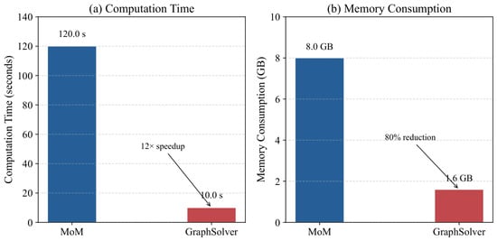
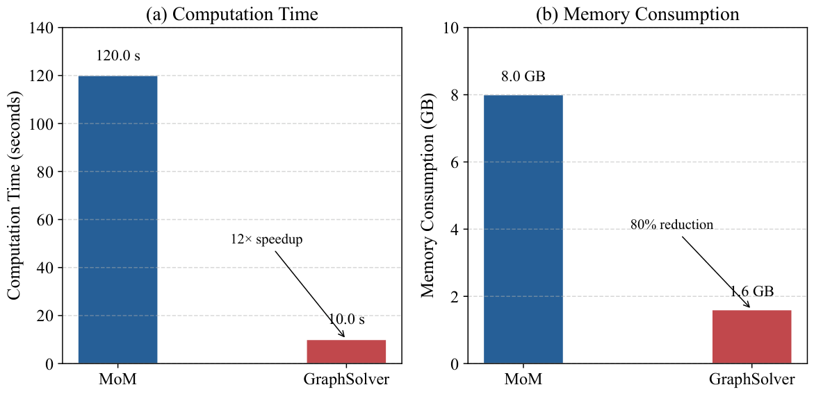
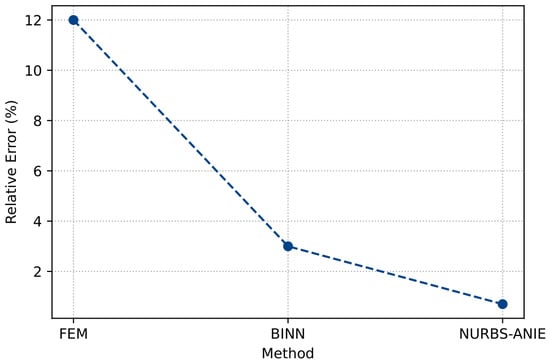
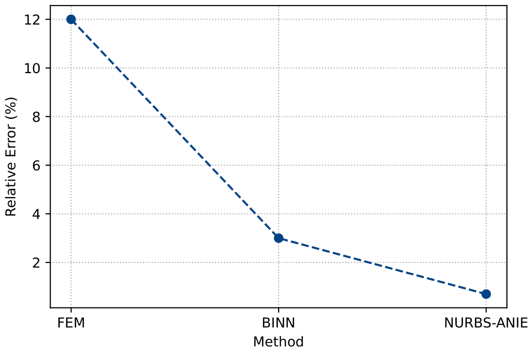
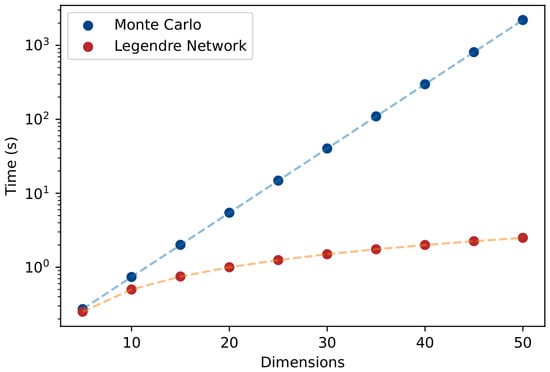
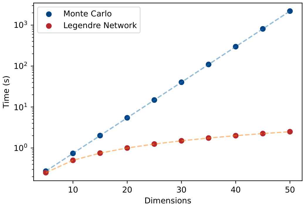
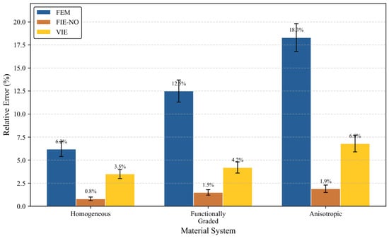
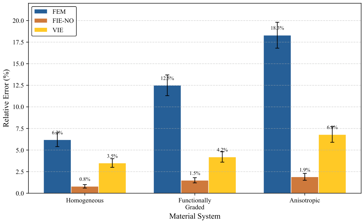

Disclaimer/Publisher’s Note: The statements, opinions and data contained in all publications are solely those of the individual author(s) and contributor(s) and not of MDPI and/or the editor(s). MDPI and/or the editor(s) disclaim responsibility for any injury to people or property resulting from any ideas, methods, instructions or products referred to in the content. |
© 2026 by the authors. Licensee MDPI, Basel, Switzerland. This article is an open access article distributed under the terms and conditions of the Creative Commons Attribution (CC BY) license.