Another Simple Proof of the Close Connection of SQS(10) and GQ(2,2) ^†

Abstract

Symmetry plays a key role in identifying the close connection between different finite incidence structures. In this paper, by studying the properties of points not belonging to an elliptic quadric of PG(3,3), a short demonstration is given of the close connection between the Steiner Quadruple system SQS(10) and the Cremona–Richmond configuration.

1. Introduction

A partially balanced incomplete block design is a triple (P,B,I), where P is a set of elements called points and B a family of sets called blocks, together with a point-block symmetric incidence relation I ⊆ P × B, where the size of P is v, the size of B is b, each point of P is contained in r blocks of B, each blocks of B contains k points of P and two points are contained in λ blocks, λ ∈ {λ₁,λ₂, …, λ_m}. A symmetric relation of association between two points is established: two points are ith associates for some i, with I ∈ {1, 2, …, m}, if they are contained in exactly ${\lambda }_i$ blocks. For this reason, a partially balanced incomplete block design is also called an m-class association scheme, cf. [1,2,3]. The number of ith associates of each point is n_i. If p and q are two points which are ith associates, then the number of points which are jth associates of p and kth associates of q is $p_{jk}^i$ and it is independent of the pair of ith associates p and q. The numbers v, b, r, k, λ₁, λ₂, …, λ_m are called parameters of first kind and the numbers n_i’s and $p_{jk}^i$’s are called parameters of second kind. They satisfy the relation: vr = bk; v ≤ b; ${\displaystyle {\sum }_{i=1}^m}{n}_i=v-1$; ${\displaystyle {\sum }_{i=1}^m}{n}_i{\lambda }_i=r\left(k-1\right)$; ${\displaystyle {\sum }_{k=1}^m}{P}_{jk}^i=n_j$ if i ≠ j; ${\displaystyle {\sum }_{k=1}^m}{P}_{jk}^i=n_j-1$ if i = j; $n_i{P}_{jk}^i=n_j{P}_{ik}^j=n_k{P}_{ij}^k$. If b = v, and so r = k, i.e., the number of points is equal to the number of lines, the partially balanced incomplete block design is said to be symmetric. Throughout the paper, we only consider connected incidence structures, where any two elements of P∪B are connected via a path of incident elements. A 2-(v,k,λ) balanced incomplete block design is a partially balanced incomplete block design where every pair of points occurs in exactly λ blocks. The parameters v, b, r, k and λ satisfy the relation: λ (v−1) = r(k−1). A (v_r,b_k)-configuration is a partially balanced incomplete block design such that two different points can be in at most one block. A symmetric configuration is denoted by (v_k). A t-(v,k,1) design is a (v_r,b_k)-configuration such that any t distinct points belong to exactly one block. A t-(v,k,1) design is called a Steiner system S (t,k,v). A S (3, q + 1, q² + 1) is said to be a finite inversive plane (also known as Möbius plane) of order q. A 3-(v,4,1) design is called a Steiner Quadruple system and denoted SQS (v). Designs exhibit many remarkable properties and appear to be closely interconnected, cf. [4,5]. A peculiar relationship in this sense occurs when one design completely determines another one, cf. [6,7]. The mutual relation between the projective plane of order four and the three-dimensional projective space of order two by the factorizations of the complete graph K₆ on six vertices was first investigated by Beutelspacher, cf. [8]. Three new geometric descriptions for one of the two projective equivalence classes of 15-sets of type (3,6)₂ in PG(3,3) were provided by Tondini in [9]. In [10] and [11], the close connection between the Desargues and the Cremona–Richmond configurations is provided. The Steiner Quadruple system with ten points, SQS(10), is one of the most important point-line incidence structures. It consists of ten points and thirty blocks, with four points on each block, twelve blocks passing through any point and at most one block through two different points. Up to isomorphism, there is a unique SQS(10); see [12]. The Cremona–Richmond configuration, also known as the generalized quadrangle GQ(2,2), is the only triangle-free symmetric (15₃) configuration. Edge was the first to describe the fundamental properties of the elliptic quadric of PG(3,3). The 30 points lying not on the elliptic quadric of PG(3,3) are joined by lines called chords. There are exactly 45 such chords. In [13], he divided the 30 points not on the quadric into two symmetric groups of 15 points and arranged each group into a set of 6 pentagons, with each of the 15 points being the common vertex of two of them. Tutte demonstrated that the 45 chords of an elliptic quadric in PG(3,3) form the edges of the highly symmetric, triangle-free cubic graph, cf. [14]. In [15], Coxeter connected the projective geometry of an elliptic quadric in PG(3,3) with the combinatorial properties of the symmetric group by proving that the automorphism group of the chords’ graph is isomorphic to the group of projective transformations under which the elliptic quadric is invariant. More recently, Brier and Bryant [16] constructed SQS(10), where the points are the ten triangle factors of K₆ and the blocks are the fifteen edges of K₆ and the fifteen 1-factors of K₆ and the close connection of SQS(10) and GQ(2,2) is given by showing that the two types of blocks correspond with the points and the lines of the Cremona–Richmond configuration. The purpose of this research is to highlight, from another point of view, the relationship between the Steiner Quadruple system with ten points and the Cremona–Richmond configuration by the incidence properties of the elliptic quadric of PG(3,3). The relation between the external points of a quadric and partially balanced incomplete block designs is not a new one and D. K. Ray-Chaudhury, in his pioneering paper [17], constructed two associate class partially incomplete block designs by linear flats contained in quadrics. In [3], the authors consider degenerate quadrics and construct a family of four-class association schemes. In [1], association schemes on the anisotropic points of classical polar spaces are studied. Geometric construction of some families of two-class and three-class association schemes from non-degenerate quadrics in characteristic two is provided in [2]. The paper is organized as follows. Section 2 introduces the preliminary result. In Section 3, by the Singer representation of PG(3,3), we obtain the two symmetric Cremona–Richmond configurations of the points not belonging to the elliptic quadric. In Section 4, by the Singer representation of PG(3,5), we obtain the two symmetric partially balanced incomplete block designs of the points not belonging to the elliptic quadric. Finally, Section 5 concludes with remarks and possible directions for future research.

2. The Incidence Properties of the Elliptic Quadric of PG(3,q), q Odd

In this section, we prove a theorem showing the close connection between a finite inversive plane of order q and a partially balanced incomplete block design. In PG(3,q), a non-degenerate quadric Q is defined by the vanishing of a quadratic form $F(x_0,x_1,x_2,x_3)$ in four variables. When q is odd, the quadric Q can be classified based on the determinant ${∆}_4$ of the associated matrix: a hyperbolic quadric Q⁺(3,q) if ${∆}_4$ is a square in ${\mathbb{F}}_q$, and an elliptic quadric Q⁻(3,q) if ${∆}_4$ is not a square in ${\mathbb{F}}_q$. When evaluating the quadratic form at a fixed point $P=(x_0,x_1,x_2,x_3)$ not lying on the quadric, the value of the quadratic form $F\left(P\right)=F(x_0,x_1,x_2,x_3)$ determines whether the point belongs to the set of squares or non-squares of the field ${\mathbb{F}}_q$. The points P not belonging to Q for which $F\left(P\right)$ is a square are called squares, while the points P not belonging to Q for which $F\left(P\right)$ is not a square are called non-squares. The polar planes with respect to Q of square points are said to be square planes, while the polar planes of non-square points are said to be non-square planes, cf. [1].

Theorem 1.

An elliptic quadric Q⁻(3,q) of PG(3,q), q odd, defines a Möbius plane and two isomorphic partially balanced incomplete block designs.

Proof. 

Let Q = Q⁻(3,q) be an elliptic quadric of PG(3,q), q odd, having quadratic form $F\left(x_0,x_1,x_2,x_3\right)$. A secant plane intersects the elliptic quadric Q in a non-singular conic containing exactly q + 1 points. Since three non-collinear points are contained in exactly one plane, the points of an elliptic quadric Q with the secant planes define a Möbius plane, i.e., a S (3, q + 1, q² + 1) Steiner system. The q (q² + 1) points of PG(3,q) not belonging to Q are partitioned into two sets of equal size: square, say S, and non-square, N. In each secant plane, the remaining q² points, not on Q, within the plane are partitioned into square and non-square points. There are q (q² + 1) secant planes in total, which are polar planes of points not belonging to Q⁻(3,q). The geometric and algebraic properties of the polar plane perfectly mirror the quadratic nature of its pole. They are divided equally into two classes: square planes and non-square planes. A square plane contains ${\displaystyle \frac{q\left(q+1\right)}{2}}$ square points and ${\displaystyle \frac{q\left(q-1\right)}{2}}$ non-square points; conversely, a non-square plane contains ${\displaystyle \frac{q\left(q-1\right)}{2}}$ square points and ${\displaystyle \frac{q\left(q+1\right)}{2}}$ non-square points. The reason for this imbalance lies in the restriction of the quadratic form to the polar plane and in the reciprocity theorem. When the quadratic form of PG(3,q) is restricted to the three-dimensional vector subspace defining the polar plane, it becomes a quadratic form in three variables of a specific type. We establish the behavior for both types of points.

If the pole is a non-zero square, the discriminant of this restricted form dictates that the non-degenerate conic behaves like a hyperbolic conic within the algebraic structure of that plane. To prove the distribution of points in the polar plane ${\pi }_P$ of a non-zero square point P, we use the algebraic properties of the bilinear form associated with the elliptic quadric in PG(3,q), q odd. Let $V={\mathbb{F}}_q^4$ be the vector space associated with PG(3,q) and let $F:V\to {\mathbb{F}}_q$ be the quadratic form defining the elliptic quadric. Let $\beta :V\times V\to {\mathbb{F}}_q$ be the symmetric bilinear form obtained by polarizing $F$:

$$\beta \left(x,y\right)={\displaystyle \frac{1}{2}}\left[F\left(x+y\right)-F\left(x\right)-F\left(y\right)\right].$$

A point P in PG(3,q) corresponds to a one-dimensional subspace $〈p〉V$.

If P is a non-zero square point, then $F\left(p\right)={\alpha }^2\in {\mathbb{F}}_q^{*}$. The polar plane ${\pi }_P$ is the three-dimensional orthogonal complement $p^{\perp }$ with respect to $\beta$:

$$p^{\perp }=\left\{x\in V:\beta \left(p,x\right)=0\right\}.$$

To analyze the points inside ${\pi }_P$, we examine the restriction of $Q$ to the three-dimensional subspace $p^{\perp }$. Let ${F|}_{p^{\perp }}$ be this restricted quadratic form. Since P does not belong to the quadric, the subspace $p^{\perp }$ does not contain p, and V decomposes into a direct sum: $V=〈p〉\oplus p^{\perp }$. For any vector $v\in V$, we can write $v=\lambda p+x$, where $\lambda \in {\mathbb{F}}_q$ and $x\in p^{\perp }$. Evaluating the global quadratic form $F$ on $v$ yields:

$$F\left(v\right)=F\left(\lambda p+x\right)={\lambda }^{2}F\left(p\right)+2\lambda \beta \left(p,x\right)+F\left(x\right).$$

Since $x\in p^{\perp }$, the cross term $2\lambda \beta \left(p,x\right)$ vanishes, simplifying to:

$$F\left(v\right)=F\left(\lambda p+x\right)={\lambda }^{2}F\left(p\right)+F\left(x\right).$$

The determinant (discriminant) of a quadratic form determines the distribution of its values. Let:

• ${∆}_4$ be the discriminant of the global form $F$ on V;
• ${∆}_3$ be the discriminant of the restricted form ${F|}_{p^{\perp }}$ on $p^{\perp }$.

From the matrix representation of the direct sum decomposition, the global discriminant factorizes as:

$${∆}_4=F\left(p\right)·{∆}_3.$$

The global discriminant ${∆}_4$ of an elliptic quadric in PG(3,q) is non–square in ${\mathbb{F}}_q$ (this is the defining algebraic property that ensures that an elliptic quadric has no lines and contains exactly q² + 1 points).

In a finite field ${\mathbb{F}}_q$, the product of a non-zero square with a non-square is always a non-square. Thus, if P is a square point, we get that $F\left(p\right)$ is square and ${∆}_3$ is non-square in ${\mathbb{F}}_q$.

A three-dimensional quadratic form over ${\mathbb{F}}_q$, with a non-square discriminant, defines a non-degenerate conic in the projective plane ${\pi }_P\cong \mathrm{P}\mathrm{G}\left(2,q\right)$. For such a ternary form $F_{p^{\perp }}$, standard finite field character sums yield the precise number of vectors $x\in p^{\perp }$ mapping to each value $z\in {\mathbb{F}}_q$. For any non-zero value $z\in {\mathbb{F}}_q^{*}$, If ${∆}_3$ is non–square in ${\mathbb{F}}_q$, the number of vector solutions to $F\left(x\right)=z$ depends on whether z matches the character of ${-∆}_3$. Since ${-∆}_3$ dictates the geometry, the number of non-zero vector solutions in $p^{\perp }$ is explicitly given by:

$$\left|\left\{x\in p^{\perp }:F\left(x\right)=z\right\}\right|=q^2-q\eta \left({-z∆}_3\right).$$

where $\eta \left(z\right)$ is the Legendre symbol, i.e., a function that equals 1 if $z$ is a square, or x1 if $z$ is a non-square.

Because ${∆}_3$ is a non-square in ${\mathbb{F}}_q$, evaluating this for all squares and non-squares in the three-dimensional subspace gives the total vector counts:

• zero vectors (on the conic): q² vectors ⇒ q + 1 projective points (since ${\displaystyle \frac{q^2-1}{q-1}}=q+1$);
• non-zero square vectors: exactly ${\displaystyle \frac{q\left(q^2-1\right)}{2}}$ vectors;
• non-square vectors: exactly ${\displaystyle \frac{q{\left(q-1\right)}^2}{2}}$ vectors.

To convert these vector counts within $p^{\perp }$ into projective points in ${\pi }_P$, we divide the non-zero vector totals by $\left(q-1\right)$:

• for non-zero square points: ${\displaystyle \frac{q\left(q^2-1\right)}{2\left(q-1\right)}}={\displaystyle \frac{q\left(q+1\right)}{2}}$;
• for non-square points: ${\displaystyle \frac{q{\left(q-1\right)}^2}{2\left(q-1\right)}}={\displaystyle \frac{q\left(q-1\right)}{2}}$.

This proves algebraically that the polar plane ${\pi }_P$ of a non-zero square point contains a surplus of exactly q square points over non-square points:

$${\displaystyle \frac{q\left(q+1\right)}{2}}-{\displaystyle \frac{q\left(q-1\right)}{2}}=q.$$

If we choose the pole P to be a non-square point, the algebraic symmetry of the finite field causes the entire distribution inside the polar plane ${\pi }_P$ to completely flip.

If P is a non-square point, then $F\left(p\right)\in {\mathbb{F}}_q^{*}$ is a non-square in ${\mathbb{F}}_q$. With the same notation as above, the global discriminant ${∆}_4$ is a non-square in ${\mathbb{F}}_q$ (because the quadric is an elliptic quadric) and $F\left(p\right)$ is a non-square (because P is a non-square point).

In a finite field ${\mathbb{F}}_q$, the product of two non-squares is always a square. Thus, if P is a non-square point, we get that $F\left(p\right)$ is non-square and ${∆}_3$ is a square in ${\mathbb{F}}_q$. When the discriminant ${∆}_3$ of a three-variable quadratic form is a square, the geometric nature of the conic section within the plane ${\pi }_P$ remains non-degenerate, still containing exactly q + 1 points. However, the internal distribution of the field values reverses. The character sum formula for the number of vector solutions in $p^{\perp }$ changes its sign behavior:

$$\left|\left\{x\in p^{\perp }:Q\left(x\right)=z\right\}\right|=q^2-q\eta \left({-z∆}_3\right)$$

Since ${∆}_3$ is a square, the character depends entirely on $-z$. This flips the counting results between squares and non-squares at the vector level:

• zero vectors (on the conic): q² vectors ⇒ q + 1 projective points (since ${\displaystyle \frac{q^2-1}{q-1}}=q+1$);
• non-zero square vectors: exactly ${\displaystyle \frac{q{\left(q-1\right)}^2}{2}}$ vectors;
• non-square vectors: exactly ${\displaystyle \frac{q\left(q^2-1\right)}{2}}$ vectors.

To convert these vector counts within $p^{\perp }$ into projective points in ${\pi }_P$, we divide the non-zero vector totals by $\left(q-1\right)$:

• for non-zero square points: ${\displaystyle \frac{q{\left(q-1\right)}^2}{2\left(q-1\right)}}={\displaystyle \frac{q\left(q-1\right)}{2}}$;
• for non-square points: ${\displaystyle \frac{q\left(q^2-1\right)}{2\left(q-1\right)}}={\displaystyle \frac{q\left(q+1\right)}{2}}$.

This proves algebraically that the polar plane ${\pi }_P$ of a non-square point contains a surplus of exactly q non-square points over non-zero square points:

$${\displaystyle \frac{q\left(q+1\right)}{2}}-{\displaystyle \frac{q\left(q-1\right)}{2}}=q.$$

This proves the beautiful reciprocity of Galois geometries: a pole always commands a majority of its own algebraic type inside its own polar plane.

To recap, in PG(3,q) with q odd, the polar plane of a point not on the elliptic quadric is a secant plane. It intersects the quadric in a non-degenerate conic containing exactly q + 1 points.

When the pole is a non-zero square point, its polar plane contains an asymmetric surplus of non-zero square points, partitioned as follows:

• q + 1 points lie on the quadric, forming the intersection conic;
• ${\displaystyle \frac{q\left(q+1\right)}{2}}$ points are non-zero squares;
• ${\displaystyle \frac{q\left(q-1\right)}{2}}$ points are non-squares.

When the pole is a non-square point, its polar plane contains an asymmetric surplus of non-square points, partitioned as follows:

• q + 1 points lie on the quadric, forming the intersection conic;
• ${\displaystyle \frac{q\left(q+1\right)}{2}}$ points are non-squares;
• ${\displaystyle \frac{q\left(q-1\right)}{2}}$ points are non-zero squares.

To determine how many square and non-square planes pass through a line $\mathcal{l}$ in PG(3,q), q odd, we must classify the line with respect to the elliptic quadric Q. In the dual two-dimensional projective space (the pencil of planes passing through a line), the classification of the planes (square or non-square) exactly reflects the signature of the points on the polar line $\mathcal{l}$^⊥. Since the quadric is elliptic, the polar line $\mathcal{l}$^⊥ always has the opposite or inverted nature relative to $\mathcal{l}$. The number of planes for each type depends exclusively on the behavior of $\mathcal{l}$ relative to Q, falling into three possible geometric cases. If $\mathcal{l}$ is external, it contains exactly ${\displaystyle \frac{\left(q+1\right)}{2}}$ square points and ${\displaystyle \frac{\left(q+1\right)}{2}}$ non-square points. By the principle of polar reciprocity, its polar line $\mathcal{l}$^⊥ is a secant line to the quadric. A secant line contains two points of the quadric, ${\displaystyle \frac{\left(q-1\right)}{2}}$ square points and ${\displaystyle \frac{\left(q-1\right)}{2}}$ non-square points. Since the planes passing through $\mathcal{l}$ correspond bijectively to the points of $\mathcal{l}$^⊥, and the classification (square/non-square) is inverted upon passing to the dual in the elliptic case, we have that exactly ${\displaystyle \frac{\left(q-1\right)}{2}}$ square planes and ${\displaystyle \frac{\left(q-1\right)}{2}}$ non-square planes pass through an external line $\mathcal{l}$. If $\mathcal{l}$ is a secant line, it contains exactly ${\displaystyle \frac{\left(q-1\right)}{2}}$ square points and ${\displaystyle \frac{\left(q-1\right)}{2}}$ non-square points. Its polar line $\mathcal{l}$^⊥ is a line external to the quadric. An external line contains exactly ${\displaystyle \frac{\left(q+1\right)}{2}}$ square points and ${\displaystyle \frac{\left(q+1\right)}{2}}$ non-square points. By reversing the nature of the points on $\mathcal{l}$^⊥ to find the planes through $\mathcal{l}$, we get that exactly ${\displaystyle \frac{\left(q+1\right)}{2}}$ square planes and ${\displaystyle \frac{\left(q+1\right)}{2}}$ non-square planes pass through a secant line $\mathcal{l}$. Now, suppose that $\mathcal{l}$ is a tangent line at a point T. If we establish a system of homogeneous coordinates in the tangent plane ${\pi }_T$ by placing the origin at T, every line passing through T can be identified by its direction. It contains exactly ${\displaystyle \frac{\left(q-1\right)}{2}}$ square points and ${\displaystyle \frac{\left(q-1\right)}{2}}$ non-square points. The tangent lines t whose direction is a square are called squares, while the tangent lines t whose direction is not a square are called non-squares. A square tangent line contains exactly ${\displaystyle \frac{\left(q+1\right)}{2}}$ square points and ${\displaystyle \frac{\left(q-1\right)}{2}}$ non-square points. A non-square tangent line contains exactly ${\displaystyle \frac{\left(q-1\right)}{2}}$ square points and ${\displaystyle \frac{\left(q+1\right)}{2}}$ non-square points.

Exactly ${\displaystyle \frac{\left(q-1\right)}{2}}$ square planes pass through a square tangent line t. This geometric result is established by applying the principle of polar reciprocity to the elliptic quadric. For an elliptic quadric, the polarity associates each tangent line r with a polar line t^⊥, which is also a tangent line sharing the same point of contact T. The key property of the elliptic polarity is that it inverts the nature of points and planes when passing to the dual space:

• The planes passing through the line t correspond bijectively to the points lying on its polar line t^⊥.
• A square point on t^⊥ corresponds to a non-square plane passing through t.
• A non-square point on t^⊥ corresponds to a square plane passing through t.
• The point of contact T (which lies on the quadric) corresponds to the unique tangent plane ${\pi }_T$.

If the tangent line t is a square tangent line, its polar line t^⊥ preserves the same geometric character, meaning it is also a square tangent line.

By applying the dual inversion rule, we can count the planes in the pencil of t based on the points of t^⊥:

○

The square planes correspond to the non-square points of t^⊥. Since there are exactly ${\displaystyle \frac{\left(q-1\right)}{2}}$ non-square points on t^⊥, there are exactly ${\displaystyle \frac{\left(q-1\right)}{2}}$ square planes in the pencil.

○

The non-square planes correspond to the square points of t^⊥. Since there are ${\displaystyle \frac{\left(q+1\right)}{2}}$ square points on t^⊥, there are ${\displaystyle \frac{\left(q+1\right)}{2}}$ non-square planes in the pencil.

Exactly ${\displaystyle \frac{\left(q-1\right)}{2}}$ square planes (and ${\displaystyle \frac{\left(q+1\right)}{2}}$) non-square planes) pass through a square tangent line.

Exactly ${\displaystyle \frac{\left(q+1\right)}{2}}$ square planes pass through a non-square tangent line t. This configuration is the dual counterpart to the previous case, operating under the same rules of elliptic polar reciprocity.

Under the polarity defined by an elliptic quadric, the nature of points and planes is inverted when shifting to the dual space:

• Planes passing through the line t correspond bijectively to the points on its polar line t^⊥.
• A square point on t^⊥ maps to a non-square plane through t.
• A non-square point on t^⊥ maps to a square plane through t.
• The contact point T on the quadric maps to the unique tangent plane ${\pi }_T$.

When the tangent line t is a non-square tangent line, its polar line t^⊥ is also a non-square tangent line passing through the same contact point T.

We determine the composition of the q + 1 planes in the pencil of t by looking at the types of points on t ^⊥ and applying the inversion rule:

• The square planes correspond directly to the non-square points on t ^⊥. Since t ^⊥ contains ${\displaystyle \frac{\left(q+1\right)}{2}}$ non-square points, there are exactly ${\displaystyle \frac{\left(q+1\right)}{2}}$ square planes passing through t.
• The non-square planes correspond to the square points on t ^⊥. Since t ^⊥ contains ${\displaystyle \frac{\left(q-1\right)}{2}}$ square points, there are exactly ${\displaystyle \frac{\left(q-1\right)}{2}}$ non-square planes passing through t.

Thus, the ${\displaystyle \frac{q\left(q^2+1\right)}{2}}$ square points with the ${\displaystyle \frac{q\left(q^2+1\right)}{2}}$ non-square planes define a symmetric partially balanced incomplete block design and the ${\displaystyle \frac{q\left(q^2+1\right)}{2}}$ non-square points with the ${\displaystyle \frac{q\left(q^2+1\right)}{2}}$ square planes define a symmetric partially balanced incomplete block design. The two designs are isomorphic. □

Since we are interested in the connection between SQS(10) and GQ(2,2), the order q must be equal to three. If q = 3, the proof of Theorem 1 ensures the existence of two isomorphic (15₃) symmetric configurations: the 15 square points with the 15 polar planes of the non–square points and the 15 non-square points with the 15 polar planes of the non–zero square points. In the next section, by the cyclic structure of the three-dimensional projective space of order three, PG(3,3), we explicitly show the two isomorphic symmetric configurations listed below in two tables.

3. The Connection Between SQS(10) and GQ(2,2)

In this section, we highlight the relationship between the Steiner Quadruple system with ten points and the Cremona–Richmond configuration by the incidence properties of the elliptic quadric of PG(3,3). To write the cyclic structure of PG(3,3), let w be a primitive element of ${{\mathbb{F}}_3}^4$ over ${\mathbb{F}}_3$ and let p (x) = x⁴ + x − 1 be its minimal polynomial over ${\mathbb{F}}_3$. The polynomial p (x) = x⁴ + x − 1 is primitive on ${\mathbb{F}}_3$. Its companion matrix C (p) is $\left(\begin{array}{cccc}0& 1& 0& 0\\ 0& 0& 1& 0\\ 0& 0& 0& 1\\ 1& -1& 0& 0\end{array}\right)$. Let us consider the point ${\omega }^0=\left(x_0,x_1,x_2,x_3\right)=\left(1,0,0,0\right).$ We get: w¹ = w⁰ C (p) = $\left(1,0,0,0\right)\left(\begin{array}{cccc}0& 1& 0& 0\\ 0& 0& 1& 0\\ 0& 0& 0& 1\\ 1& -1& 0& 0\end{array}\right)=\left(0,1,0,0\right)$; by continuing in this way and by denoting the points represented by wⁱ simply by i, we obtain the cyclic structure of PG(3,3), as listed in

Table 1. The cyclic structure of the points of PG(3,3).

w0 = (1,0,0,0) = 0	w1 = (0,1,0,0) = 1	w2 = (0,0,1,0) = 2	w3 = (0,0,0,1) = 3
w4 = (1,−1,0,0) = 4	w5 = (0,1,−1,0) = 5	w6 = (0,0,1,−1) = 6	w7 = (1,−1,0,−1) = 7
w8 = (1,1,1,0) = 8	w9 = (0,1,1,1) = 9	w10 = (1,−1,1,1) = 10	w11 = (1,0,−1,1) = 11
w12 = (1,0,0,−1) = 12	w13 = (1,1,0,0) = 13	w14 = (0,1,1,0) = 14	w15 = (0,0,1,1) = 15
w16 = (1,−1,0,1) = 16	w17 = (1,0,−1,0) = 17	w18 = (0,1,0,−1) = 18	w19 = (1,−1,−1,0) = 19
w20 = (0,1,−1,−1) = 20	w21 = (1,−1,−1,1) = 21	w22 = (1,0,−1,−1) = 22	w23 = (1,1,0,1) = 23
w24 = (1,0,1,0) = 24	w25 = (0,1,0,1) = 25	w26 = (1,−1,1,0) = 26	w27 = (0,1,−1,1) = 27
w28 = (1,−1,1,−1) = 28	w29 = (1,1,1,−1) = 29	w30 = (1,1,−1,−1) = 30	w31 = (1,1,−1,1) = 31
w32 = (1,0,1,−1) = 32	w33 = (1,1,0,−1) = 33	w34 = (1,1,−1,0) = 34	w35 = (0,1,1,−1) = 35
w36 = (1,−1,−1,−1) = 36	w37 = (1,1,1,1) = 37	w38 = (1,0,1,1) = 38	w39 = (1,0,0,1) = 39

. Thus, the Singer group is isomorphic to the additive group Z₄₀, the integers modulo 40.

Since under the action of a cyclic collineation group of a finite projective space, the point set and the plane set have the same cyclic structure, select any plane; for example, we choose the plane π₀: = x₀ = 0, which contains the 13-set of points listed in

Table 2. The starting plane.

π0

1

2

3

5

6

9

14

15

18

20

25

27

35

, where the first entry is the label of the plane label, not a point, and the others 13 entries are the points of the plane. Note that the plane π₀ does not contain the point 0 because the equation of π₀ is x₀ = 0, while the point 0 has homogeneous coordinate x₀ = 1.

The remaining planes of space are found by adding 1 to each point of the preceding plane, beginning with π₀ and using addition modulo 40. Let us consider an elliptic quadric Q⁻(3,3) of PG(3,3). The canonical equation of Q⁻(3,3) is $Q\left(x_0,x_1,x_2,x_3\right)=x_0^2+x_0{x}_1-x_1^2+x_2{x}_3=0$. Let us color the points of PG(3,3) with red, blue, and green. Red, if they belong to the elliptic quadric, that is, if the quadratic form evaluates to zero; blue, if the quadratic form evaluates to a non-zero square; and green, if the quadratic form evaluates to a non-square. The colored points are listed in

Table 3. The colored points.

Q(1,0,0,0) = 1⇒0	Q(0,1,0,0) = −1⇒1	Q(0,0,1,0) = 0⇒2	Q(0,0,0,1) = 0⇒3
Q(1,−1,0,0) = −1⇒4	Q(0,1,−1,0) = −1⇒5	Q(0,0,1,−1) = −1⇒6	Q(1,−1,0,−1) = −1⇒7
Q(1,1,1,0) = 1⇒8	Q(0,1,1,1) = 0⇒9	Q(1,−1,1,1) = 0⇒10	Q(1,0,−1,1) = 0⇒11
Q(1,0,0,−1) = 1⇒12	Q(1,1,0,0) = 1⇒13	Q(0,1,1,0) = −1⇒14	Q(0,0,1,1) = 1⇒15
Q(1,−1,0,1) = −1⇒16	Q(1,0,−1,0) = 1⇒17	Q(0,1,0,−1) = −1⇒18	Q(1,−1,−1,0) = −1⇒19
Q(0,1,−1,−1) = 0⇒20	Q(1,−1,−1,1) = 1⇒21	Q(1,0,−1,−1) = −1⇒22	Q(1,1,0,1) = 1⇒23
Q(1,0,1,0) = 1⇒24	Q(0,1,0,1) = −1⇒25	Q(1,−1,1,0) = −1⇒26	Q(0,1,−1,1) = 1⇒27
Q(1,−1,1,−1) = 1⇒28	Q(1,1,1,−1) = 0⇒29	Q(1,1,−1,−1) = −1⇒30	Q(1,1,−1,1) = 0⇒31
Q(1,0,1,−1) = 0⇒32	Q(1,1,0,−1) = 1⇒33	Q(1,1,−1,0) = 1⇒34	Q(0,1,1,−1) = 1⇒35
Q(1,−1,−1,−1) = 0⇒36	Q(1,1,1,1) = −1⇒37	Q(1,0,1,1) = −1⇒38	Q(1,0,0,1) = 1⇒39

.

We get three sets of points:

N = {1, 4, 5, 6, 7, 14, 16, 18, 19, 22, 25, 26, 30, 37, 38}.

Q = {2, 3, 9, 10, 11, 20, 29, 31, 32, 36}.

S = {0, 8, 12, 13, 15, 17, 21, 23, 24, 27, 28, 33, 34, 35, 39}.

The colored points of the planes of PG(3,3) are listed in the rows of

Table 4. The colored points of the planes of PG(3,3).

π0	1	2	3	5	6	9	14	15	18	20	25	27	35
π1	2	3	4	6	7	10	15	16	19	21	26	28	36
π2	3	4	5	7	8	11	16	17	20	22	27	29	37
π3	4	5	6	8	9	12	17	18	21	23	28	30	38
π4	5	6	7	9	10	13	18	19	22	24	29	31	39
π5	0	6	7	8	10	11	14	19	20	23	25	30	32
π6	1	7	8	9	11	12	15	20	21	24	26	31	33
π7	2	8	9	10	12	13	16	21	22	25	27	32	34
π8	3	9	10	11	13	14	17	22	23	26	28	33	35
π9	4	10	11	12	14	15	18	23	24	27	29	34	36
π10	5	11	12	13	15	16	19	24	25	28	30	35	37
π11	6	12	13	14	16	17	20	25	26	29	31	36	38
π12	7	13	14	15	17	18	21	26	27	30	32	37	39
π13	0	8	14	15	16	18	19	22	27	28	31	33	38
π14	1	9	15	16	17	19	20	23	28	29	32	34	39
π15	0	2	10	16	17	18	20	21	24	29	30	33	35
π16	1	3	11	17	18	19	21	22	25	30	31	34	36
π17	2	4	12	18	19	20	22	23	26	31	32	35	37
π18	3	5	13	19	20	21	23	24	27	32	33	36	38
π19	4	6	14	20	21	22	24	25	28	33	34	37	39
π20	0	5	7	15	21	22	23	25	26	29	34	35	38
π21	1	6	8	16	22	23	24	26	27	30	35	36	39
π22	0	2	7	9	17	23	24	25	27	28	31	36	37
π23	1	3	8	10	18	24	25	26	28	29	32	37	38
π24	2	4	9	11	19	25	26	27	29	30	33	38	39
π25	0	3	5	10	12	20	26	27	28	30	31	34	39
π26	0	1	4	6	11	13	21	27	28	29	31	32	35
π27	1	2	5	7	12	14	22	28	29	30	32	33	36
π28	2	3	6	8	13	15	23	29	30	31	33	34	37
π29	3	4	7	9	14	16	24	30	31	32	34	35	38
π30	4	5	8	10	15	17	25	31	32	33	35	36	39
π31	0	5	6	9	11	16	18	26	32	33	34	36	37
π32	1	6	7	10	12	17	19	27	33	34	35	37	38
π33	2	7	8	11	13	18	20	28	34	35	36	38	39
π34	0	3	8	9	12	14	19	21	29	35	36	37	39
π35	0	1	4	9	10	13	15	20	22	30	36	37	38
π36	1	2	5	10	11	14	16	21	23	31	37	38	39
π37	0	2	3	6	11	12	15	17	22	24	32	38	39
π38	0	1	3	4	7	12	13	16	18	23	25	33	39
π39	0	1	2	4	5	8	13	14	17	19	24	26	34

, where the first entry is the label of the plane label, not a point, and the others 13 entries are the points of the plane.

The elliptic quadric Q⁻(3,3) defines a polarity

$$P:=\left(y_0,y_1,y_2,y_3\right)\to \pi :=\left(y_0-y_1\right)x_0-\left(y_0+y_1\right)x_1-y_3{x}_2-y_2{x}_3=0$$

Let us color the planes of PG(3,3) with red, blue, and green. Red, if the plane is the polar plane of a point belonging to the elliptic quadric; blue, if it is the polar plane of a non-zero square point; and green, if it is the polar plane of a non-square point. The colored planes of PG(3,3) are listed in

Table 5. The colored planes of PG(3,3).

0 = (1,0,0,0)⇒$x_0{x}_1$⇒π28	1 = (0,1,0,0)⇒$x_0{+x}_1=0$⇒π1
2 = (0,0,1,0)⇒$x_{3}0$⇒π39	3 = (0,0,0,1)⇒$x_{2}0$⇒π38
4 = (1,−1,0,0)⇒$x_{0}0$⇒π0	5 = (0,1,−1,0)⇒$x_0+x_1{x}_3$⇒π24
6 = (0,0,1,−1)⇒$x_2{x}_3$⇒π35	7 = (1,−1,0,−1)⇒$x_0{x}_2$⇒π23
8= (1,1,1,0)⇒$x_1{x}_3$⇒π22	9 = (0,1,1,1)⇒$x_0+x_1+{x_2+x}_3=0$⇒π3
10 = (1,−1,1,1)⇒$x_0+{x_2+x}_3=0$⇒π32	11 = (1,0,−1,1)⇒$x_0+x_3={x_1+x}_2$⇒π10
12 = (1,0,0,−1)⇒$x_0+x_2=x_1$⇒π8	13 = (1,1,0,0)⇒$x_{1}0$⇒π37
14=(0,1,1,0)⇒$x_0+{x_1+x}_3=0$⇒π17	15 = (0,0,1,1)⇒$x_2{+x}_3=0$⇒π26
16 = (1,−1,0,1)⇒$x_0{+x}_2=0$⇒π16	17 = (1,0,−1,0)⇒$x_0+x_3=x_1$⇒π7
18 = (0,1,0,−1)⇒$x_0+x_1{x}_2$⇒π29	19 = (1,−1,−1,0)⇒$x_0{x}_3$⇒π36
20 = (0,1,−1,−1)⇒$x_0+x_1={x_2+x}_3$⇒π19	21 = (1,−1,−1,1)⇒$x_0+x_2{x}_3$⇒π14
22 = (1,0,−1,−1)⇒$x_0+x_2+x_3{x}_1$⇒π11	23 = (1,1,0,1)⇒$x_1{x}_2$⇒ π34
24 = (1,0,1,0)⇒$x_0=x_1+x_3$⇒π33	25 = (0,1,0,1)⇒$x_0+{x_1+x}_2=0$⇒π2
26 = (1,−1,1,0)⇒$x_0{+x}_3=0$⇒π27	27 = (0,1,−1,1)⇒$x_0+x_1+x_2{x}_3$⇒π30
28 = (1,−1,1,−1)⇒$x_0+x_3=x_2$⇒π6	29 = (1,1,1,−1)⇒$x_1+x_2=x_3$⇒π20
30 = (1,1,−1,−1)⇒$x_1+{x_2+x}_3=0$⇒π31	31 = (1,1,−1,1)⇒$x_1+x_3=x_2$⇒π13
32 = (1,0,1,−1)⇒$x_0+x_2={x_1+x}_3$⇒π12	33 = (1,1,0,−1)⇒$x_1{+x}_2=0$⇒π25
34 = (1,1,−1,0)⇒$x_1{+x}_3=0$⇒π15	35 = (0,1,1,−1)⇒$x_0+x_1+x_3{x}_2$⇒π9
36 = (1,−1,−1,−1)⇒$x_0={x_2+x}_3$⇒π21	37 = (1,1,1,1)⇒$x_2+x_3=x_1$⇒π5
38 = (1,0,1,1)⇒$x_1+x_2+x_3{x}_0$⇒π4	39 = (1,0,0,1)⇒$x_0={x_1+x}_2$⇒π18

.

Let us consider the green points of the blue planes listed in

Table 6. The points and the blocks of the green Cremona–Richmond configuration.

N = {1, 4, 5, 6, 7, 14, 16, 18, 19, 22, 25, 26, 30, 37, 38}.
π6	π7	π8	π9	π14	π15	π18	π22	π25	π26	π28	π30	π33	π34	π37
1	16	14	4	1	16	5	7	5	1	6	4	7	14	6
7	22	22	14	16	18	19	25	26	4	30	5	18	19	22
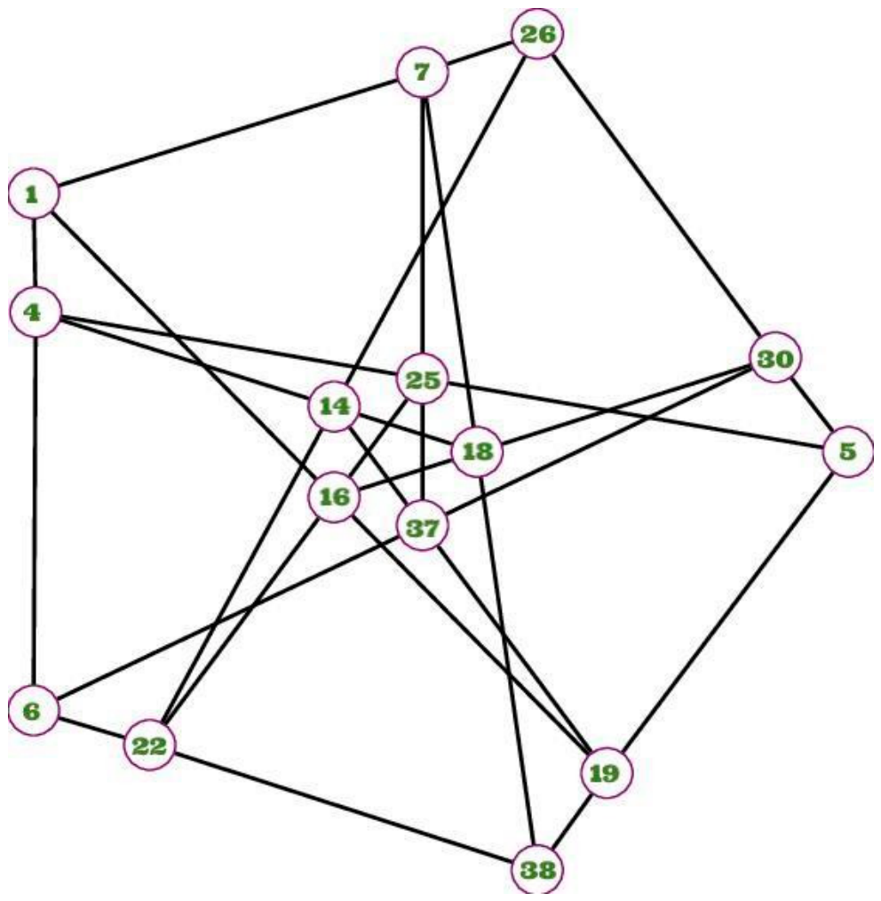
26	25	26	18	19	30	38	37	30	6	37	25	38	37	38

. It is simple to verify that we get a Cremona–Richmond configuration by the direct representation in Figure 1.

Let us consider the red points of the blue and green planes listed in

Table 7. The points and the blocks of the SQS(10).

Q = {2, 3, 9, 10, 11, 20, 29, 31, 32, 36}.
π0	π1	π2	π4	π5	π6	π7	π8	π9	π11	π14	π15	π16	π17	π18
2	2	3	9	10	9	2	3	10	20	9	2	3	2	3
3	3	11	10	11	11	9	9	11	29	20	10	11	20	20
9	10	20	29	20	20	10	10	29	31	29	20	31	31	32
20	36	29	31	32	31	32	11	36	36	32	29	36	32	36
π22	π23	π24	π25	π26	π27	π28	π29	π30	π31	π33	π34	π35	π36	π37
2	3	2	3	11	2	2	3	10	9	2	3	9	2	2
9	10	9	10	29	29	3	9	31	11	11	9	10	10	3
31	29	11	20	31	32	29	31	32	32	20	29	20	11	11
36	32	29	31	32	36	31	32	36	36	36	36	36	31	32

. It is easy to verify that we get a SQS(10).

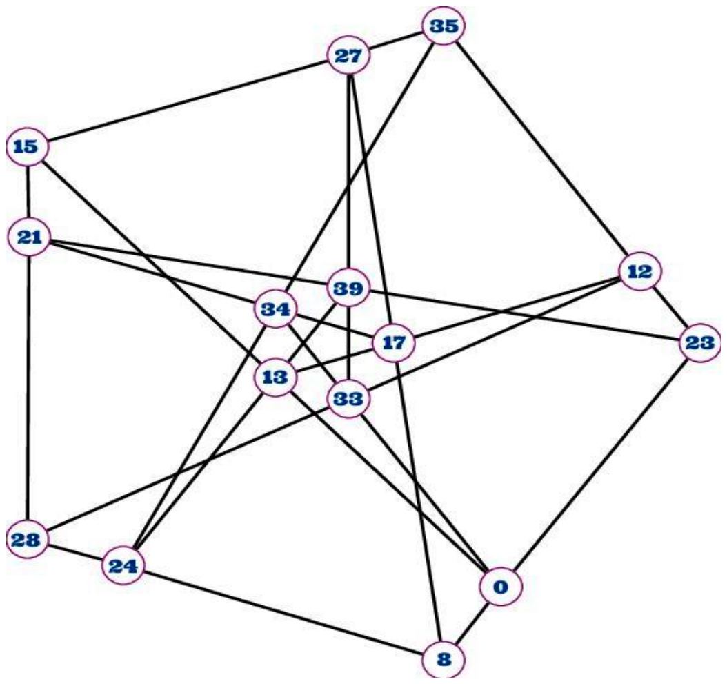
Now, let us consider the blue points of the green planes listed in

Table 8. The points and the blocks of the blue Cremona–Richmond configuration.

S = {0, 8, 12, 13, 15, 17, 21, 23, 24, 27, 28, 33, 34, 35, 39}.
π0	π1	π2	π4	π5	π11	π16	π17	π23	π24	π27	π29	π31	π35	π36
15	15	8	13	0	12	17	12	8	27	12	24	0	0	21
27	21	17	24	8	13	21	23	24	33	28	34	33	13	23
35	28	27	39	23	17	34	35	28	39	33	35	34	15	39

. It is simple to verify that we get a Cremona–Richmond configuration by the direct representation in Figure 2.

For the next odd order, q = 5, the proof of Theorem 1 ensures the existence of two isomorphic symmetric partially balanced incomplete block designs: the 65 square points with the 65 polar planes of the non-square points and the 65 non-square points with the 65 polar planes of the non-zero square points. In the next section, by the cyclic structure of the three-dimensional projective space of order five, PG(3,5), we explicitly show the two isomorphic symmetric partially balanced incomplete block designs listed below in two tables.

4. The Connection Between the Steiner System S(3,6,26) and a Symmetric (65,10) Point-Block Incidence Structure

In this section, we highlight the relationship between the Steiner Quadruple system with twenty-six points and two isomorphic symmetric partially balanced incomplete block designs by the incidence properties of the elliptic quadric of PG(3,5). The finite inversive plane of order five, S(3,6,26), is unique, cf. [18] and [19]. It consists of twenty-six points and one hundred and thirty blocks, with six points on each block, thirty blocks passing through any point and exactly six blocks through two different points. To write the cyclic structure of PG(3,5), let w be a primitive element of ${{\mathbb{F}}_5}^4$ over ${\mathbb{F}}_5$ and let p (x) = x⁴ + x² + 2x + 2 be its minimal polynomial over ${\mathbb{F}}_5$. The polynomial p (x) = x⁴ + x² + 2x + 2 is primitive on ${\mathbb{F}}_5$. The companion matrix C (p) is $\left(\begin{array}{cccc}0& 1& 0& 0\\ 0& 0& 1& 0\\ 0& 0& 0& 1\\ 3& 3& 4& 0\end{array}\right)$. Let us consider the point ${\omega }^0=\left(x_0,x_1,x_2,x_3\right)=\left(1,0,0,0\right).$ We get: w¹ = w⁰ C (p) = $\left(1,0,0,0\right)\left(\begin{array}{cccc}0& 1& 0& 0\\ 0& 0& 1& 0\\ 0& 0& 0& 1\\ 3& 3& 4& 0\end{array}\right)=\left(0,1,0,0\right)$; by continuing in this way and by denoting the points represented by wⁱ simply by i, we obtain the cyclic structure of PG(3,5), as listed in

Table 9. The cyclic structure of the colored points of PG(3,5).

ω0 = (1,0,0,0) = 0	ω1= (0,1,0,0) = 1	ω2 = (0,0,1,0) = 2	ω3 = (0,0,0,1) = 3
ω4 = (1,1,3,0) = 4	ω5 = (0,1,1,3) = 5	ω6 = (1,1,2,4) = 6	ω7 = (1,4,1,1) = 7
ω8 = (1,3,1,2) = 8	ω9 = (1,2,1,1) = 9	ω10 = (1,3,2,2) = 10	ω11 = (1,2,1,2) = 11
ω12 = (1,2,0,1) = 12	ω13 = (1,3,2,0) = 13	ω14 = (0,1,3,2) = 14	ω15 = (1,1,4,3) = 15
ω16 = (1,0,2,1) = 16	ω17= (1,3,3,4) = 17	ω18 = (1,4,2,4) = 18	ω19 = (1,4,0,1) = 19
ω20 = (1,3,1,0) = 20	ω21 = (0,1,3,1) = 21	ω22 = (1,1,0,1) = 22	ω23 = (1,3,0,0) = 23
ω24 = (0,1,3,0) = 24	ω25 = (0,0,1,3) = 25	ω26 = (1,1,3,4) = 26	ω27 = (1,4,1,4) = 27
ω28 = (1,4,0,3) = 28	ω29 = (1,0,4,0) = 29	ω30 = (0,1,0,4) = 30	ω31 = (1,1,1,0) = 31
ω32 = (0,1,1,1) = 32	ω33 = (1,1,0,2) = 33	ω34 = (1,2,4,0) = 34	ω35 = (0,1,2,4) = 35
ω36 = (1,1,1,1) = 36	ω37 = (1,3,0,2) = 37	ω38 = (1,2,1,0) = 38	ω39 = (0,1,2,1) = 39
ω40 = (1,1,0,4) = 40	ω41 = (1,4,1,0) = 41	ω42 = (0,1,4,1) = 42	ω43 = (1,1,0,3) = 43
ω44 = (1,0,2,0) = 44	ω45 = (0,1,0,2) = 45	ω46 = (1,1,4,0) = 46	ω47 = (0,1,1,4) = 47
ω48 = (1,1,1,3) = 48	ω49 = (1,0,2,4) = 49	ω50 = (1,4,3,1) = 50	ω51 = (1,3,1,1) = 51
ω52 = (1,3,4,2) = 52	ω53 = (1,2,1,4) = 53	ω54 = (1,4,4,3) = 54	ω55 = (1,0,4,1) = 55
ω56 = (1,3,3,3) = 56	ω57 = (1,0,0,2) = 57	ω58 = (1,2,3,0) = 58	ω59 = (0,1,2,3) = 59
ω60 = (1,1,2,3) = 60	ω61 = (1,0,2,3) = 61	ω62 = (1,0,3,3) = 62	ω63 = (1,0,3,2) = 63
ω64 = (1,2,3,3) = 64	ω65 = (1,0,1,2) = 65	ω66 = (1,2,3,1) = 66	ω67 = (1,3,2,1) = 67
ω68 = (1,3,4,4) = 68	ω69 = (1,4,2,2) = 69	ω70 = (1,2,2,2) = 70	ω71 = (1,2,0,2) = 71
ω72 = (1,2,0,0) = 72	ω73 = (0,1,2,0) = 73	ω74 = (0,0,1,2) = 74	ω75 = (1,1,3,1) = 75
ω76 = (1,3,0,1) = 76	ω77 = (1,3,4,0) = 77	ω78 = (0,1,3,4) = 78	ω79 = (1,1,1,4) = 79
ω80 = (1,4,1,3) = 80	ω81 = (1,0,4,4) = 81	ω82 = (1,4,3,2) = 82	ω83 = (1,2,2,3) = 83
ω84 = (1,0,1,3) = 84	ω85 = (1,0,3,4) = 85	ω86 = (1,4,3,4) = 86	ω87 = (1,4,0,4) = 87
ω88 = (1,4,0,0) = 88	ω89 = (0,1,4,0) = 89	ω90 = (0,0,1,4) = 90	ω91 = (1,1,3,3) = 91
ω92 = (1,0,2,2) = 92	ω93 = (1,2,3,2) = 93	ω94 = (1,2,0,3) = 94	ω95 = (1,0,1,0) = 95
ω96 = (0,1,0,1) = 96	ω97 = (1,1,0,0) = 97	ω98 = (0,1,1,0) = 98	ω99 = (0,0,1,1) = 99
ω100 = (1,1,3,2) = 100	ω101 = (1,2,4,3) = 101	ω102 = (1,0,1,1) = 102	ω103 = (1,3,3,2) = 103
ω104 = (1,2,1,3) = 104	ω105 = (1,0,1,4) = 105	ω106 = (1,4,3,3) = 106	ω107 = (1,0,4,2) = 107
ω108 = (1,2,3,4) = 108	ω109 = (1,4,4,4) = 109	ω110 = (1,4,0,2) = 110	ω111 = (1,2,2,0) = 111
ω112 = (0,1,2,2) = 112	ω113 = (1,1,4,2) = 113	ω114 = (1,2,4,4) = 114	ω115 = (1,4,4,2) = 115
ω116 = (1,2,2,4) = 116	ω117 = (1,4,4,1) = 117	ω118 = (1,3,1,3) = 118	ω119 = (1,0,0,4) = 119
ω120 = (1,4,3,0) = 120	ω121 = (0,1,4,3) = 121	ω122 = (1,1,2,1) = 122	ω123 = (1,3,0,4) = 123
ω124 = (1,4,2,0) = 124	ω125 = (0,1,4,2) = 125	ω126 = (1,1,4,4) = 126	ω127 = (1,4,1,2) = 127
ω128 = (1,2,2,1) = 128	ω129 = (1,3,2,4) = 129	ω130 = (1,4,2,1) = 130	ω131 = (1,3,1,4) = 131
ω132 = (1,4,2,3) = 132	ω133 = (1,0,4,3) = 133	ω134 = (1,0,3,1) = 134	ω135 = (1,3,3,1) = 135
ω136 = (1,3,4,1) = 136	ω137 = (1,3,4,3) = 137	ω138 = (1,0,0,1) = 138	ω139 = (1,3,3,0) = 139
ω140 = (0,1,3,3) = 140	ω141 = (1,1,2,2) = 141	ω142 = (1,2,4,2) = 142	ω143 = (1,2,0,4) = 143
ω144 = (1,4,4,0) = 144	ω145 = (0,1,4,4) = 145	ω146 = (1,1,1,2) = 146	ω147 = (1,2,4,1) = 147
ω148 = (1,3,2,3) = 148	ω149 = (1,0,0,3) = 149	ω150 = (1,0,3,0) = 150	ω151 = (0,1,0,3) = 151
ω152 = (1,1,2,0) = 152	ω153 = (0,1,1,2) = 153	ω154 = (1,1,4,1) = 154	ω155 = (1,3,0,3) = 155

. Thus, the Singer group is isomorphic to the additive group Z₁₅₆, the integers modulo 156. Let us consider an elliptic quadric Q⁻(3,5) of PG(3,5). The canonical equation of Q⁻(3,5) is $Q\left(x_0,x_1,x_2,x_3\right)=x_0^2+x_1^2+x_2^2+2x_3^2=0$. Let us color the points of PG(3,5) with red, blue, and green. Red, if they belong to the elliptic quadric, that is, if the quadratic form evaluates to zero; blue, if the quadratic form evaluates to a non-zero square; and green, if the quadratic form evaluates to a non-square. The colored points are listed in Table 9.

We get three sets of points:

N = {3, 6, 9, 10, 12, 14, 16, 18, 21, 26, 29, 30, 31, 35, 37, 39, 41, 46, 49, 50, 51, 53, 56, 59, 61, 62, 63, 64, 68, 70, 71, 75, 76, 78, 83, 85, 86, 88, 89, 90, 92, 93, 94, 95, 96, 97, 98, 99, 103, 112, 114, 119, 122, 123, 130, 131, 134, 136, 138, 140, 143, 144, 147, 148, 155}.

Q = {5, 7, 23, 24, 27, 28, 33, 36, 43, 44, 65, 72, 73, 79, 84, 107, 109, 110, 117, 121, 125, 126, 133, 150, 153, 154}.

S = {0, 1, 2, 4, 8, 11, 13, 15, 17, 19, 20, 22, 25, 32, 34, 38, 40, 42, 45, 47, 48, 52, 54, 55, 57, 58, 60, 66, 67, 69, 74, 77, 80, 81, 82, 87, 91, 100, 101, 102, 104, 105, 106, 108, 111, 113, 115, 116, 118, 120, 124, 127, 128, 129, 132, 135, 137, 139, 141, 142, 145, 146, 149, 151, 152}.

Since under the action of a cyclic collineation group of a finite projective space, the point set and the plane set have the same cyclic structure, select any plane; for example, we choose the plane π₀: = x₀ = 0, which contains the 31-set of points listed in

Table 10. The starting plane of PG(3,5).

π0	1	2	3	5	14	21	24	25	30	32	35	39	42	45	47
59	73	74	78	89	90	96	98	99	112	121	125	140	145	151	153

, where the first entry is the label of the plane label, not a point, and the others 31 entries are the points of the plane. Note that the plane π₀ does not contain the point 0 because the equation of π₀ is x₀ = 0, while the point 0 has homogeneous coordinate x₀ = 1.

The remaining planes of space are found by adding 1 to each point of the preceding plane, beginning with π₀ and using addition modulo 156. The colored points of the planes of PG(3,5) are listed in the rows of

Table A1. The colored points of the planes of PG(3,5).

π0	1	2	3	5	14	21	24	25	30	32	35	39	42	45	47
59	73	74	78	89	90	96	98	99	112	121	125	140	145	151	153
π1	2	3	4	6	15	22	25	26	31	33	36	40	43	46	48
60	74	75	79	90	91	97	99	100	113	122	126	141	146	152	154
π2	3	4	5	7	16	23	26	27	32	34	37	41	44	47	49
61	75	76	80	91	92	98	100	101	114	123	127	142	147	153	155
π3	0	4	5	6	8	17	24	27	28	33	35	38	42	45	48
50	62	76	77	81	92	93	99	101	102	115	124	128	143	148	154
π4	1	5	6	7	9	18	25	28	29	34	36	39	43	46	49
51	63	77	78	82	93	94	100	102	103	116	125	129	144	149	155
π5	0	2	6	7	8	10	19	26	29	30	35	37	40	44	47
50	52	64	78	79	83	94	95	101	103	104	117	126	130	145	150
π6	1	3	7	8	9	11	20	27	30	31	36	38	41	45	48
51	53	65	79	80	84	95	96	102	104	105	118	127	131	146	151
π7	2	4	8	9	10	12	21	28	31	32	37	39	42	46	49
52	54	66	80	81	85	96	97	103	105	106	119	128	132	147	152
π8	3	5	9	10	11	13	22	29	32	33	38	40	43	47	50
53	55	67	81	82	86	97	98	104	106	107	120	129	133	148	153
π9	4	6	10	11	12	14	23	30	33	34	39	41	44	48	51
54	56	68	82	83	87	98	99	105	107	108	121	130	134	149	154
π10	5	7	11	12	13	15	24	31	34	35	40	42	45	49	52
55	57	69	83	84	88	99	100	106	108	109	122	131	135	150	155
π11	0	6	8	12	13	14	16	25	32	35	36	41	43	46	50
53	56	58	70	84	85	89	100	101	107	109	110	123	132	136	151
π12	1	7	9	13	14	15	17	26	33	36	37	42	44	47	51
54	57	59	71	85	86	90	101	102	108	110	111	124	133	137	152
π13	2	8	10	14	15	16	18	27	34	37	38	43	45	48	52
55	58	60	72	86	87	91	102	103	109	111	112	125	134	138	153
π14	3	9	11	15	16	17	19	28	35	38	39	44	46	49	53
56	59	61	73	87	88	92	103	104	110	112	113	126	135	139	154
π15	4	10	12	16	17	18	20	29	36	39	40	45	47	50	54
57	60	62	74	88	89	93	104	105	111	113	114	127	136	140	155
π16	0	5	11	13	17	18	19	21	30	37	40	41	46	48	51
55	58	61	63	75	89	90	94	105	106	112	114	115	128	137	141
π17	1	6	12	14	18	19	20	22	31	38	41	42	47	49	52
56	59	62	64	76	90	91	95	106	107	113	115	116	129	138	142
π18	2	7	13	15	19	20	21	23	32	39	42	43	48	50	53
57	60	63	65	77	91	92	96	107	108	114	116	117	130	139	143
π19	3	8	14	16	20	21	22	24	33	40	43	44	49	51	54
58	61	64	66	78	92	93	97	108	109	115	117	118	131	140	144
π20	4	9	15	17	21	22	23	25	34	41	44	45	50	52	55
59	62	65	67	79	93	94	98	109	110	116	118	119	132	141	145
π21	5	10	16	18	22	23	24	26	35	42	45	46	51	53	56
60	63	66	68	80	94	95	99	110	111	117	119	120	133	142	146
π22	6	11	17	19	23	24	25	27	36	43	46	47	52	54	57
61	64	67	69	81	95	96	100	111	112	118	120	121	134	143	147
π23	7	12	18	20	24	25	26	28	37	44	47	48	53	55	58
62	65	68	70	82	96	97	101	112	113	119	121	122	135	144	148
π24	8	13	19	21	25	26	27	29	38	45	48	49	54	56	59
63	66	69	71	83	97	98	102	113	114	120	122	123	136	145	149
π25	9	14	20	22	26	27	28	30	39	46	49	50	55	57	60
64	67	70	72	84	98	99	103	114	115	121	123	124	137	146	150
π26	10	15	21	23	27	28	29	31	40	47	50	51	56	58	61
65	68	71	73	85	99	100	104	115	116	122	124	125	138	147	151
π27	11	16	22	24	28	29	30	32	41	48	51	52	57	59	62
66	69	72	74	86	100	101	105	116	117	123	125	126	139	148	152
π28	12	17	23	25	29	30	31	33	42	49	52	53	58	60	63
67	70	73	75	87	101	102	106	117	118	124	126	127	140	149	153
π29	13	18	24	26	30	31	32	34	43	50	53	54	59	61	64
68	71	74	76	88	102	103	107	118	119	125	127	128	141	150	154
π30	14	19	25	27	31	32	33	35	44	51	54	55	60	62	65
69	72	75	77	89	103	104	108	119	120	126	128	129	142	151	155
π31	0	15	20	26	28	32	33	34	36	45	52	55	56	61	63
66	70	73	76	78	90	104	105	109	120	121	127	129	130	143	152
π32	1	16	21	27	29	33	34	35	37	46	53	56	57	62	64
67	71	74	77	79	91	105	106	110	121	122	128	130	131	144	153
π33	2	17	22	28	30	34	35	36	38	47	54	57	58	63	65
68	72	75	78	80	92	106	107	111	122	123	129	131	132	145	154
π34	3	18	23	29	31	35	36	37	39	48	55	58	59	64	66
69	73	76	79	81	93	107	108	112	123	124	130	132	133	146	155
π35	0	4	19	24	30	32	36	37	38	40	49	56	59	60	65
67	70	74	77	80	82	94	108	109	113	124	125	131	133	134	147
π36	1	5	20	25	31	33	37	38	39	41	50	57	60	61	66
68	71	75	78	81	83	95	109	110	114	125	126	132	134	135	148
π37	2	6	21	26	32	34	38	39	40	42	51	58	61	62	67
69	72	76	79	82	84	96	110	111	115	126	127	133	135	136	149
π38	3	7	22	27	33	35	39	40	41	43	52	59	62	63	68
70	73	77	80	83	85	97	111	112	116	127	128	134	136	137	150
π39	4	8	23	28	34	36	40	41	42	44	53	60	63	64	69
71	74	78	81	84	86	98	112	113	117	128	129	135	137	138	151
π40	5	9	24	29	35	37	41	42	43	45	54	61	64	65	70
72	75	79	82	85	87	99	113	114	118	129	130	136	138	139	152
π41	6	10	25	30	36	38	42	43	44	46	55	62	65	66	71
73	76	80	83	86	88	100	114	115	119	130	131	137	139	140	153
π42	7	11	26	31	37	39	43	44	45	47	56	63	66	67	72
74	77	81	84	87	89	101	115	116	120	131	132	138	140	141	154
π43	8	12	27	32	38	40	44	45	46	48	57	64	67	68	73
75	78	82	85	88	90	102	116	117	121	132	133	139	141	142	155
π44	0	9	13	28	33	39	41	45	46	47	49	58	65	68	69
74	76	79	83	86	89	91	103	117	118	122	133	134	140	142	143
π45	1	10	14	29	34	40	42	46	47	48	50	59	66	69	70
75	77	80	84	87	90	92	104	118	119	123	134	135	141	143	144
π46	2	11	15	30	35	41	43	47	48	49	51	60	67	70	71
76	78	81	85	88	91	93	105	119	120	124	135	136	142	144	145
π47	3	12	16	31	36	42	44	48	49	50	52	61	68	71	72
77	79	82	86	89	92	94	106	120	121	125	136	137	143	145	146
π48	4	13	17	32	37	43	45	49	50	51	53	62	69	72	73
78	80	83	87	90	93	95	107	121	122	126	137	138	144	146	147
π49	5	14	18	33	38	44	46	50	51	52	54	63	70	73	74
79	81	84	88	91	94	96	108	122	123	127	138	139	145	147	148
π50	6	15	19	34	39	45	47	51	52	53	55	64	71	74	75
80	82	85	89	92	95	97	109	123	124	128	139	140	146	148	149
π51	7	16	20	35	40	46	48	52	53	54	56	65	72	75	76
81	83	86	90	93	96	98	110	124	125	129	140	141	147	149	150
π52	8	17	21	36	41	47	49	53	54	55	57	66	73	76	77
82	84	87	91	94	97	99	111	125	126	130	141	142	148	150	151
π53	9	18	22	37	42	48	50	54	55	56	58	67	74	77	78
83	85	88	92	95	98	100	112	126	127	131	142	143	149	151	152
π54	10	19	23	38	43	49	51	55	56	57	59	68	75	78	79
84	86	89	93	96	99	101	113	127	128	132	143	144	150	152	153
π55	11	20	24	39	44	50	52	56	57	58	60	69	76	79	80
85	87	90	94	97	100	102	114	128	129	133	144	145	151	153	154
π56	12	21	25	40	45	51	53	57	58	59	61	70	77	80	81
86	88	91	95	98	101	103	115	129	130	134	145	146	152	154	155
π57	0	13	22	26	41	46	52	54	58	59	60	62	71	78	81
82	87	89	92	96	99	102	104	116	130	131	135	146	147	153	155
π58	0	1	14	23	27	42	47	53	55	59	60	61	63	72	79
82	83	88	90	93	97	100	103	105	117	131	132	136	147	148	154
π59	1	2	15	24	28	43	48	54	56	60	61	62	64	73	80
83	84	89	91	94	98	101	104	106	118	132	133	137	148	149	155
π60	0	2	3	16	25	29	44	49	55	57	61	62	63	65	74
81	84	85	90	92	95	99	102	105	107	119	133	134	138	149	150
π61	1	3	4	17	26	30	45	50	56	58	62	63	64	66	75
82	85	86	91	93	96	100	103	106	108	120	134	135	139	150	151
π62	2	4	5	18	27	31	46	51	57	59	63	64	65	67	76
83	86	87	92	94	97	101	104	107	109	121	135	136	140	151	152
π63	3	5	6	19	28	32	47	52	58	60	64	65	66	68	77
84	87	88	93	95	98	102	105	108	110	122	136	137	141	152	153
π64	4	6	7	20	29	33	48	53	59	61	65	66	67	69	78
85	88	89	94	96	99	103	106	109	111	123	137	138	142	153	154
π65	5	7	8	21	30	34	49	54	60	62	66	67	68	70	79
86	89	90	95	97	100	104	107	110	112	124	138	139	143	154	155
π66	0	6	8	9	22	31	35	50	55	61	63	67	68	69	71
80	87	90	91	96	98	101	105	108	111	113	125	139	140	144	155
π67	0	1	7	9	10	23	32	36	51	56	62	64	68	69	70
72	81	88	91	92	97	99	102	106	109	112	114	126	140	141	145
π68	1	2	8	10	11	24	33	37	52	57	63	65	69	70	71
73	82	89	92	93	98	100	103	107	110	113	115	127	141	142	146
π69	2	3	9	11	12	25	34	38	53	58	64	66	70	71	72
74	83	90	93	94	99	101	104	108	111	114	116	128	142	143	147
π70	3	4	10	12	13	26	35	39	54	59	65	67	71	72	73
75	84	91	94	95	100	102	105	109	112	115	117	129	143	144	148
π71	4	5	11	13	14	27	36	40	55	60	66	68	72	73	74
76	85	92	95	96	101	103	106	110	113	116	118	130	144	145	149
π72	5	6	12	14	15	28	37	41	56	61	67	69	73	74	75
77	86	93	96	97	102	104	107	111	114	117	119	131	145	146	150
π73	6	7	13	15	16	29	38	42	57	62	68	70	74	75	76
78	87	94	97	98	103	105	108	112	115	118	120	132	146	147	151
π74	7	8	14	16	17	30	39	43	58	63	69	71	75	76	77
79	88	95	98	99	104	106	109	113	116	119	121	133	147	148	152
π75	8	9	15	17	18	31	40	44	59	64	70	72	76	77	78
80	89	96	99	100	105	107	110	114	117	120	122	134	148	149	153
π76	9	10	16	18	19	32	41	45	60	65	71	73	77	78	79
81	90	97	100	101	106	108	111	115	118	121	123	135	149	150	154
π77	10	11	17	19	20	33	42	46	61	66	72	74	78	79	80
82	91	98	101	102	107	109	112	116	119	122	124	136	150	151	155
π78	0	11	12	18	20	21	34	43	47	62	67	73	75	79	80
81	83	92	99	102	103	108	110	113	117	120	123	125	137	151	152
π79	1	12	13	19	21	22	35	44	48	63	68	74	76	80	81
82	84	93	100	103	104	109	111	114	118	121	124	126	138	152	153
π80	2	13	14	20	22	23	36	45	49	64	69	75	77	81	82
83	85	94	101	104	105	110	112	115	119	122	125	127	139	153	154
π81	3	14	15	21	23	24	37	46	50	65	70	76	78	82	83
84	86	95	102	105	106	111	113	116	120	123	126	128	140	154	155
π82	0	4	15	16	22	24	25	38	47	51	66	71	77	79	83
84	85	87	96	103	106	107	112	114	117	121	124	127	129	141	155
π83	0	1	5	16	17	23	25	26	39	48	52	67	72	78	80
84	85	86	88	97	104	107	108	113	115	118	122	125	128	130	142
π84	1	2	6	17	18	24	26	27	40	49	53	68	73	79	81
85	86	87	89	98	105	108	109	114	116	119	123	126	129	131	143
π85	2	3	7	18	19	25	27	28	41	50	54	69	74	80	82
86	87	88	90	99	106	109	110	115	117	120	124	127	130	132	144
π86	3	4	8	19	20	26	28	29	42	51	55	70	75	81	83
87	88	89	91	100	107	110	111	116	118	121	125	128	131	133	145
π87	4	5	9	20	21	27	29	30	43	52	56	71	76	82	84
88	89	90	92	101	108	111	112	117	119	122	126	129	132	134	146
π88	5	6	10	21	22	28	30	31	44	53	57	72	77	83	85
89	90	91	93	102	109	112	113	118	120	123	127	130	133	135	147
π89	6	7	11	22	23	29	31	32	45	54	58	73	78	84	86
90	91	92	94	103	110	113	114	119	121	124	128	131	134	136	148
π90	7	8	12	23	24	30	32	33	46	55	59	74	79	85	87
91	92	93	95	104	111	114	115	120	122	125	129	132	135	137	149
π91	8	9	13	24	25	31	33	34	47	56	60	75	80	86	88
92	93	94	96	105	112	115	116	121	123	126	130	133	136	138	150
π92	9	10	14	25	26	32	34	35	48	57	61	76	81	87	89
93	94	95	97	106	113	116	117	122	124	127	131	134	137	139	151
π93	10	11	15	26	27	33	35	36	49	58	62	77	82	88	90
94	95	96	98	107	114	117	118	123	125	128	132	135	138	140	152
π94	11	12	16	27	28	34	36	37	50	59	63	78	83	89	91
95	96	97	99	108	115	118	119	124	126	129	133	136	139	141	153
π95	12	13	17	28	29	35	37	38	51	60	64	79	84	90	92
96	97	98	100	109	116	119	120	125	127	130	134	137	140	142	154
π96	13	14	18	29	30	36	38	39	52	61	65	80	85	91	93
97	98	99	101	110	117	120	121	126	128	131	135	138	141	143	155
π97	0	14	15	19	30	31	37	39	40	53	62	66	81	86	92
94	98	99	100	102	111	118	121	122	127	129	132	136	139	142	144
π98	1	15	16	20	31	32	38	40	41	54	63	67	82	87	93
95	99	100	101	103	112	119	122	123	128	130	133	137	140	143	145
π99	2	16	17	21	32	33	39	41	42	55	64	68	83	88	94
96	100	101	102	104	113	120	123	124	129	131	134	138	141	144	146
π100	3	17	18	22	33	34	40	42	43	56	65	69	84	89	95
97	101	102	103	105	114	121	124	125	130	132	135	139	142	145	147
π101	4	18	19	23	34	35	41	43	44	57	66	70	85	90	96
98	102	103	104	106	115	122	125	126	131	133	136	140	143	146	148
π102	5	19	20	24	35	36	42	44	45	58	67	71	86	91	97
99	103	104	105	107	116	123	126	127	132	134	137	141	144	147	149
π103	6	20	21	25	36	37	43	45	46	59	68	72	87	92	98
100	104	105	106	108	117	124	127	128	133	135	138	142	145	148	150
π104	7	21	22	26	37	38	44	46	47	60	69	73	88	93	99
101	105	106	107	109	118	125	128	129	134	136	139	143	146	149	151
π105	8	22	23	27	38	39	45	47	48	61	70	74	89	94	100
102	106	107	108	110	119	126	129	130	135	137	140	144	147	150	152
π106	9	23	24	28	39	40	46	48	49	62	71	75	90	95	101
103	107	108	109	111	120	127	130	131	136	138	141	145	148	151	153
π107	10	24	25	29	40	41	47	49	50	63	72	76	91	96	102
104	108	109	110	112	121	128	131	132	137	139	142	146	149	152	154
π108	11	25	26	30	41	42	48	50	51	64	73	77	92	97	103
105	109	110	111	113	122	129	132	133	138	140	143	147	150	153	155
π109	0	12	26	27	31	42	43	49	51	52	65	74	78	93	98
104	106	110	111	112	114	123	130	133	134	139	141	144	148	151	154
π110	1	13	27	28	32	43	44	50	52	53	66	75	79	94	99
105	107	111	112	113	115	124	131	134	135	140	142	145	149	152	155
π111	0	2	14	28	29	33	44	45	51	53	54	67	76	80	95
100	106	108	112	113	114	116	125	132	135	136	141	143	146	150	153
π112	1	3	15	29	30	34	45	46	52	54	55	68	77	81	96
101	107	109	113	114	115	117	126	133	136	137	142	144	147	151	154
π113	2	4	16	30	31	35	46	47	53	55	56	69	78	82	97
102	108	110	114	115	116	118	127	134	137	138	143	145	148	152	155
π114	0	3	5	17	31	32	36	47	48	54	56	57	70	79	83
98	103	109	111	115	116	117	119	128	135	138	139	144	146	149	153
π115	1	4	6	18	32	33	37	48	49	55	57	58	71	80	84
99	104	110	112	116	117	118	120	129	136	139	140	145	147	150	154
π116	2	5	7	19	33	34	38	49	50	56	58	59	72	81	85
100	105	111	113	117	118	119	121	130	137	140	141	146	148	151	155
π117	0	3	6	8	20	34	35	39	50	51	57	59	60	73	82
86	101	106	112	114	118	119	120	122	131	138	141	142	147	149	152
π118	1	4	7	9	21	35	36	40	51	52	58	60	61	74	83
87	102	107	113	115	119	120	121	123	132	139	142	143	148	150	153
π119	2	5	8	10	22	36	37	41	52	53	59	61	62	75	84
88	103	108	114	116	120	121	122	124	133	140	143	144	149	151	154
π120	3	6	9	11	23	37	38	42	53	54	60	62	63	76	85
89	104	109	115	117	121	122	123	125	134	141	144	145	150	152	155
π121	0	4	7	10	12	24	38	39	43	54	55	61	63	64	77
86	90	105	110	116	118	122	123	124	126	135	142	145	146	151	153
π122	1	5	8	11	13	25	39	40	44	55	56	62	64	65	78
87	91	106	111	117	119	123	124	125	127	136	143	146	147	152	154
π123	2	6	9	12	14	26	40	41	45	56	57	63	65	66	79
88	92	107	112	118	120	124	125	126	128	137	144	147	148	153	155
π124	0	3	7	10	13	15	27	41	42	46	57	58	64	66	67
80	89	93	108	113	119	121	125	126	127	129	138	145	148	149	154
π125	1	4	8	11	14	16	28	42	43	47	58	59	65	67	68
81	90	94	109	114	120	122	126	127	128	130	139	146	149	150	155
π126	0	2	5	9	12	15	17	29	43	44	48	59	60	66	68
69	82	91	95	110	115	121	123	127	128	129	131	140	147	150	151
π127	1	3	6	10	13	16	18	30	44	45	49	60	61	67	69
70	83	92	96	111	116	122	124	128	129	130	132	141	148	151	152
π128	2	4	7	11	14	17	19	31	45	46	50	61	62	68	70
71	84	93	97	112	117	123	125	129	130	131	133	142	149	152	153
π129	3	5	8	12	15	18	20	32	46	47	51	62	63	69	71
72	85	94	98	113	118	124	126	130	131	132	134	143	150	153	154
π130	4	6	9	13	16	19	21	33	47	48	52	63	64	70	72
73	86	95	99	114	119	125	127	131	132	133	135	144	151	154	155
π131	0	5	7	10	14	17	20	22	34	48	49	53	64	65	71
73	74	87	96	100	115	120	126	128	132	133	134	136	145	152	155
π132	0	1	6	8	11	15	18	21	23	35	49	50	54	65	66
72	74	75	88	97	101	116	121	127	129	133	134	135	137	146	153
π133	1	2	7	9	12	16	19	22	24	36	50	51	55	66	67
73	75	76	89	98	102	117	122	128	130	134	135	136	138	147	154
π134	2	3	8	10	13	17	20	23	25	37	51	52	56	67	68
74	76	77	90	99	103	118	123	129	131	135	136	137	139	148	155
π135	0	3	4	9	11	14	18	21	24	26	38	52	53	57	68
69	75	77	78	91	100	104	119	124	130	132	136	137	138	140	149
π136	1	4	5	10	12	15	19	22	25	27	39	53	54	58	69
70	76	78	79	92	101	105	120	125	131	133	137	138	139	141	150
π137	2	5	6	11	13	16	20	23	26	28	40	54	55	59	70
71	77	79	80	93	102	106	121	126	132	134	138	139	140	142	151
π138	3	6	7	12	14	17	21	24	27	29	41	55	56	60	71
72	78	80	81	94	103	107	122	127	133	135	139	140	141	143	152
π139	4	7	8	13	15	18	22	25	28	30	42	56	57	61	72
73	79	81	82	95	104	108	123	128	134	136	140	141	142	144	153
π140	5	8	9	14	16	19	23	26	29	31	43	57	58	62	73
74	80	82	83	96	105	109	124	129	135	137	141	142	143	145	154
π141	6	9	10	15	17	20	24	27	30	32	44	58	59	63	74
75	81	83	84	97	106	110	125	130	136	138	142	143	144	146	155
π142	0	7	10	11	16	18	21	25	28	31	33	45	59	60	64
75	76	82	84	85	98	107	111	126	131	137	139	143	144	145	147
π143	1	8	11	12	17	19	22	26	29	32	34	46	60	61	65
76	77	83	85	86	99	108	112	127	132	138	140	144	145	146	148
π144	2	9	12	13	18	20	23	27	30	33	35	47	61	62	66
77	78	84	86	87	100	109	113	128	133	139	141	145	146	147	149
π145	3	10	13	14	19	21	24	28	31	34	36	48	62	63	67
78	79	85	87	88	101	110	114	129	134	140	142	146	147	148	150
π146	4	11	14	15	20	22	25	29	32	35	37	49	63	64	68
79	80	86	88	89	102	111	115	130	135	141	143	147	148	149	151
π147	5	12	15	16	21	23	26	30	33	36	38	50	64	65	69
80	81	87	89	90	103	112	116	131	136	142	144	148	149	150	152
π148	6	13	16	17	22	24	27	31	34	37	39	51	65	66	70
81	82	88	90	91	104	113	117	132	137	143	145	149	150	151	153
π149	7	14	17	18	23	25	28	32	35	38	40	52	66	67	71
82	83	89	91	92	105	114	118	133	138	144	146	150	151	152	154
π150	8	15	18	19	24	26	29	33	36	39	41	53	67	68	72
83	84	90	92	93	106	115	119	134	139	145	147	151	152	153	155
π151	0	9	16	19	20	25	27	30	34	37	40	42	54	68	69
73	84	85	91	93	94	107	116	120	135	140	146	148	152	153	154
π152	1	10	17	20	21	26	28	31	35	38	41	43	55	69	70
74	85	86	92	94	95	108	117	121	136	141	147	149	153	154	155
π153	0	2	11	18	21	22	27	29	32	36	39	42	44	56	70
71	75	86	87	93	95	96	109	118	122	137	142	148	150	154	155
π154	0	1	3	12	19	22	23	28	30	33	37	40	43	45	57
71	72	76	87	88	94	96	97	110	119	123	138	143	149	151	155
π155	0	1	2	4	13	20	23	24	29	31	34	38	41	44	46
58	72	73	77	88	89	95	97	98	111	120	124	139	144	150	152

, Appendix A, where the first entry is the label of the plane label, not a point, and the others 31 entries are the points of the plane. Let us consider the green points of the blue planes listed in Table A1. A direct check shows that we get a symmetric partially balanced incomplete block design with parameters v = b = 65 r = k = 10, m = 3, λ₁ = 0, λ₂ = 2, λ₃ = 3, n₁ = 24, n₂ = 30, n₃ = 10, $P_{23}^1=5$, $P_{13}^2=4$, and $P_{12}^3=12$, whose points and blocks are listed in the rows of

Table 11. The points and the blocks of the green symmetric partially balanced incomplete block design.

π1	3	6	26	31	46	75	90	97	99	122
π3	6	35	50	62	76	92	93	99	143	148
π6	3	9	30	31	41	51	53	95	96	131
π8	3	9	10	29	50	53	86	97	98	148
π10	12	31	35	49	83	88	99	122	131	155
π12	9	14	26	37	51	59	71	85	86	90
π13	10	14	16	18	37	86	103	112	134	138
π18	21	39	50	53	63	92	96	114	130	143
π20	9	21	41	50	59	62	93	94	98	119
π22	6	46	61	64	95	96	112	134	143	147
π27	16	29	30	41	51	59	62	86	123	148
π28	12	29	30	31	49	53	63	70	75	140
π30	14	31	35	51	62	75	89	103	119	155
π31	26	56	61	63	70	76	78	90	130	143
π33	30	35	63	68	75	78	92	122	123	131
π35	30	37	49	56	59	70	94	131	134	147
π37	6	21	26	39	51	61	62	76	96	136
π39	41	53	63	64	71	78	86	98	112	138
π42	26	31	37	39	56	63	89	131	138	140
π43	12	46	64	68	75	78	85	88	90	155
π52	21	41	49	53	76	94	97	99	130	148
π55	39	50	56	76	85	90	94	97	114	144
π59	56	61	62	64	83	89	94	98	148	155
π63	3	6	64	68	88	93	95	98	122	136
π68	10	37	63	70	71	89	92	93	98	103
π71	14	68	76	85	92	95	96	103	130	144
π76	9	10	16	18	41	71	78	90	97	123
π77	10	46	61	78	98	112	119	122	136	155
π78	12	18	21	62	75	83	92	99	103	123
π79	12	21	35	63	68	76	93	103	114	138
π80	14	49	64	75	83	85	94	112	119	122
π82	16	51	71	83	85	96	103	112	114	155
π83	16	26	39	78	85	86	88	97	122	130
π85	3	18	41	50	86	88	90	99	130	144
π86	3	26	29	51	70	75	83	88	89	131
π90	12	30	46	59	85	92	93	95	114	122
π100	3	18	56	89	95	97	103	114	130	147
π102	35	71	86	97	99	103	123	134	144	147
π103	6	21	37	46	59	68	92	98	138	148
π104	21	26	37	46	88	93	99	134	136	143
π105	39	61	70	89	94	119	130	140	144	147
π107	10	29	41	49	50	63	76	96	112	131
π110	50	53	75	94	99	112	131	134	140	155
π111	14	29	51	53	76	95	112	114	136	143
π112	3	29	30	46	68	96	114	136	144	147
π114	3	31	56	70	83	98	103	119	138	144
π115	6	18	37	49	71	99	112	136	140	147
π116	49	50	56	59	85	119	130	140	148	155
π118	9	21	35	51	61	83	119	123	143	148
π121	10	12	39	61	63	64	86	90	122	123
π122	39	56	62	64	78	119	123	136	143	147
π124	3	10	41	46	64	89	93	119	138	148
π125	14	16	59	68	90	94	114	122	130	155
π126	9	12	29	59	68	95	123	131	140	147
π131	10	14	49	53	64	71	96	134	136	155
π132	6	18	21	35	49	50	75	88	97	134
π136	10	12	39	53	70	76	78	92	131	138
π137	6	16	26	59	70	71	93	134	138	140
π139	18	30	56	61	95	123	134	136	140	144
π140	9	14	16	26	29	31	62	83	96	143
π144	9	12	18	30	35	61	62	78	86	147
π148	6	16	31	37	39	51	70	88	90	143
π149	14	18	35	71	83	89	92	114	138	144
π151	9	16	30	37	68	85	93	94	140	148
π155	29	31	41	46	88	89	95	97	98	144

.

Let us consider the red points of the blue and green planes listed in Table A1. It is easy to verify, by checking

Table 12. The points and the blocks of the S(3,6,26).

π0	π1	π2	π3	π4	π5	π6	π8	π9	π10	π11	π12	π13
5	33	5	5	5	7	7	5	23	5	36	7	27
24	36	7	24	7	44	27	33	33	7	43	33	43
73	43	23	27	28	79	36	43	44	24	84	36	72
121	79	27	28	36	117	65	107	107	84	107	44	109
125	126	44	33	43	126	79	133	121	109	109	110	125
153	154	153	154	125	150	84	153	154	150	110	133	153
π14	π18	π19	π20	π21	π22	π23	π25	π26	π27	π28	π29	π30
28	7	24	23	5	23	7	27	23	24	23	24	27
44	23	33	44	23	24	24	28	27	28	33	43	33
73	43	43	65	24	27	28	72	28	72	73	107	44
110	65	44	79	110	36	44	84	65	117	117	125	65
126	107	109	109	117	43	65	121	73	125	126	150	72
154	117	117	110	133	121	121	150	125	126	153	154	126
π31	π32	π33	π34	π35	π36	π37	π38	π39	π40	π41	π42	π43
28	27	28	23	24	5	72	7	23	5	36	7	27
33	33	36	36	36	33	79	27	28	24	43	43	44
36	79	65	73	65	109	84	33	36	43	44	44	73
73	110	72	79	109	110	110	43	44	65	65	72	117
109	121	107	107	125	125	126	73	84	72	73	84	121
121	153	154	133	133	126	133	150	117	79	153	154	133
π44	π47	π48	π49	π51	π52	π54	π55	π58	π59	π60	π62	π63
28	36	43	5	7	36	23	24	23	24	44	5	5
33	44	72	33	65	73	43	44	27	28	65	27	28
65	72	73	44	72	84	79	79	72	43	84	65	65
79	79	107	73	110	125	84	133	79	73	107	107	84
117	121	121	79	125	126	150	153	117	84	133	109	110
133	125	126	84	150	150	153	154	154	133	150	121	153
π64	π65	π67	π68	π70	π71	π72	π74	π75	π76	π77	π78	π79
7	5	7	24	65	5	5	7	44	65	33	43	44
33	7	23	33	72	27	28	43	72	73	72	73	84
65	79	36	65	73	36	73	79	107	79	79	79	109
109	107	72	73	84	72	107	109	110	121	107	110	121
153	110	109	107	109	73	117	121	117	150	109	117	126
154	154	126	110	117	110	150	133	153	154	150	125	153
π80	π81	π82	π83	π84	π85	π86	π87	π88	π89	π90	π91	π93
23	23	24	5	24	7	28	5	5	7	7	24	27
36	24	79	23	27	27	107	27	28	23	23	33	33
110	65	84	72	73	28	110	43	44	73	24	121	36
125	84	107	84	79	109	121	84	72	84	33	126	107
153	126	117	107	109	110	125	117	109	110	79	133	117
154	154	121	125	126	117	133	126	133	121	125	150	125
π94	π95	π96	π100	π101	π102	π103	π104	π105	π106	π107	π108	π109
27	28	36	33	23	5	36	7	23	23	24	73	27
28	79	65	43	43	24	43	44	27	24	72	109	43
36	84	110	65	44	36	72	73	107	28	109	110	65
126	109	117	84	125	44	117	107	110	107	110	133	110
133	125	121	121	126	107	133	109	126	109	121	150	133
153	154	126	125	133	126	150	125	150	153	154	153	154
π110	π111	π112	π114	π115	π116	π118	π119	π120	π121	π122	π123	π124
27	28	107	5	33	5	7	5	23	7	5	65	7
28	33	109	36	84	7	36	36	109	24	44	79	27
43	44	117	79	110	33	107	84	117	43	65	107	121
44	125	126	109	117	72	121	121	121	110	117	125	125
79	150	133	117	150	117	150	133	125	126	125	126	126
107	153	154	153	154	121	153	154	150	153	154	153	154
π125	π126	π128	π129	π130	π131	π132	π133	π136	π137	π138	π139	π140
28	5	7	5	33	5	23	7	5	5	7	7	5
43	43	84	72	72	7	65	24	27	23	24	28	23
65	44	117	126	73	65	72	36	79	28	27	72	43
109	110	125	150	125	73	121	73	125	79	72	73	73
126	121	133	153	133	126	133	117	133	121	107	79	109
150	150	153	154	154	133	153	154	150	126	133	153	154
π141	π142	π144	π145	π147	π148	π149	π150	π151	π152	π153	π154	π155
24	7	23	24	5	24	7	24	27	28	27	23	23
27	28	27	28	23	27	23	33	73	43	36	28	24
44	33	33	36	33	65	28	36	84	117	44	33	44
84	84	84	79	36	117	133	72	107	121	109	43	72
110	107	109	110	65	150	150	84	153	153	150	72	73
125	126	133	150	150	153	154	153	154	154	154	110	150

, that the finite inversive plane of order five, S(3,6,26), is obtained.

Let us consider the blue points of the green planes listed in Table A1. A direct check shows that we get a symmetric partially balanced incomplete block design with parameters v = b = 65 r = k = 10, m = 3, λ₁ = 0, λ₂ = 2, λ₃ = 3, n₁ = 24, n₂ = 30, n₃ = 10, $P_{23}^1=5$, $P_{13}^2=4$, and $P_{12}^3=12$, whose points and blocks are listed in the rows of

Table 13. The points and the blocks of the blue symmetric partially balanced incomplete block design.

π0	1	2	25	32	42	45	47	74	145	151
π2	4	32	34	47	80	91	100	101	127	142
π4	1	25	34	77	82	100	102	116	129	149
π5	0	2	8	19	40	47	52	101	104	145
π9	4	11	34	48	54	82	87	105	108	149
π11	0	8	13	25	32	58	100	101	132	151
π14	11	15	17	19	38	87	104	113	135	139
π19	8	20	22	40	54	58	66	108	115	118
π21	22	42	45	60	66	80	111	120	142	146
π23	20	25	47	48	55	58	82	101	113	135
π25	20	22	55	57	60	67	115	124	137	146
π26	15	40	47	58	100	104	115	116	124	151
π29	13	32	34	54	74	102	118	127	128	141
π32	1	34	57	67	74	77	91	105	106	128
π34	48	55	58	66	69	81	108	124	132	146
π36	1	20	25	38	57	60	66	81	132	135
π38	22	40	52	77	80	111	116	127	128	137
π40	42	45	54	82	87	113	118	129	139	152
π41	25	38	42	55	66	80	100	115	137	139
π44	0	13	45	47	58	69	74	91	118	142
π47	42	48	52	77	82	106	120	137	145	146
π48	4	13	17	32	45	69	80	87	137	146
π49	38	52	54	74	81	91	108	127	139	145
π51	20	40	48	52	54	81	124	129	141	149
π54	19	38	55	57	101	113	127	128	132	152
π58	0	1	42	47	55	60	82	100	105	132
π60	0	2	25	55	57	74	81	102	105	149
π62	2	4	57	67	87	101	104	135	151	152
π64	4	20	48	66	67	69	106	111	137	142
π65	8	34	54	60	66	67	100	104	124	139
π67	0	1	32	69	81	91	102	106	141	145
π70	4	13	54	67	91	100	102	105	115	129
π72	15	67	69	74	77	102	104	111	145	146
π74	8	17	58	69	77	104	106	113	116	152
π75	8	15	17	40	77	80	100	105	120	149
π81	15	82	102	105	106	111	113	116	120	128
π84	1	2	17	40	81	87	105	108	116	129
π87	4	20	52	82	101	108	111	129	132	146
π88	22	57	77	91	102	113	118	120	127	135
π89	11	22	32	45	54	58	91	113	124	128
π91	8	13	25	34	47	60	80	105	115	116
π93	11	15	58	77	82	118	128	132	135	152
π94	11	34	91	108	115	118	124	129	139	141
π95	13	17	38	60	100	116	120	127	137	142
π96	13	38	52	80	91	101	120	128	135	141
π101	4	19	34	57	66	102	104	106	115	146
π106	40	48	101	108	111	120	127	141	145	151
π108	11	25	42	48	77	105	111	113	129	132
π109	0	42	52	74	104	106	111	139	141	151
π119	2	8	22	52	108	116	120	124	149	151
π120	11	38	42	54	60	104	115	141	145	152
π123	2	40	45	57	66	118	120	124	128	137
π128	2	4	11	17	19	45	129	142	149	152
π129	8	15	20	32	47	69	113	118	124	132
π130	4	13	19	47	48	52	127	132	135	151
π133	1	2	19	22	55	66	67	102	128	135
π138	17	55	60	80	81	127	135	139	141	152
π141	15	17	20	32	58	74	81	106	142	146
π142	0	11	25	45	60	82	111	137	139	145
π145	13	19	34	48	67	87	101	129	142	146
π147	15	38	69	80	81	87	116	142	149	152
π150	8	15	19	67	106	115	139	145	151	152
π152	1	17	20	38	55	69	74	108	141	149
π153	0	2	11	22	32	42	87	118	137	142
π154	0	1	19	22	40	45	57	87	149	151

.

5. Concluding Remarks

We have investigated the close connection between the SQS(10) and the Cremona–Richmond configuration. Using the incidence properties of the points not belonging to the elliptic quadric of PG(3,3) with the secant planes, we obtained two symmetric GQ(2,2). Similarly, by the incidence properties of the points not belonging to the elliptic quadric of PG(3,5) with the secant planes, we obtained two symmetric partially balanced incomplete block design with parameters v = b = 65 r = k = 10, m = 3, λ₁ = 0, λ₂ = 2, λ₃ = 3, n₁ = 24, n₂ = 30, n₃ = 10, $P_{23}^1=5$, $P_{13}^2=4$, and $P_{12}^3=12$. We believe that the techniques developed in this paper may inspire future investigation involving similar manipulation of incidence properties applicable to classical algebraic varieties with the aim of obtaining other symmetric partially balanced incomplete block designs.