The Unit Extended Exponential Distribution: Properties, Inference and Applications

Abstract

In this paper, we introduce a new probability distribution defined on the unit interval $(0,1)$, called the unit extended exponential (UEE) distribution. The proposed model is obtained through a transformation of a random variable following the extended exponential distribution, leading to a flexible family able to describe skewed and boundary-concentrated data. The structural properties of this distribution are derived, including its density, cumulative distribution, survival, hazard rate and quantile function, along with the mode and moments. A characterization based on its hazard function is also presented. Parameter estimation is performed via maximum likelihood. Under standard regularity conditions, the asymptotic properties of the estimators are established. A Monte Carlo simulation study is carried out to assess the finite-sample performance of the estimators. Finally, the usefulness of the model is illustrated through two applications to real proportion data, where our proposal is compared with competing models such as the unit-Lindley and Beta distributions using information criteria. The results suggest that the proposed distribution provides a competitive and often superior fit.

1. Introduction

The statistical analysis of random variables restricted to the unit interval $(0,1)$ represents a persistent challenge across various applied disciplines. In fields such as biostatistics, econometrics, reliability engineering and environmental sciences, it is common to encounter measurements structured as proportions, rates, probabilities or indices. Unlike continuous data defined over the entire real line, observations within the unit interval frequently exhibit pronounced skewness and, quite often, a strong concentration of probability mass near the boundary limits (zero or one). These structural characteristics render traditional Gaussian models inadequate, necessitating the development of specialized distributions.

Historically, the Beta distribution has served as the benchmark model for this type of data due to its remarkable geometric flexibility [1], which allows it to assume U shapes, J shapes or inverted asymmetries. However, its practical application is hindered by certain analytical drawbacks. The most notable limitation is the absence of a closed-form analytical expression for its cumulative distribution function, which relies directly on the incomplete Beta function. This mathematical hurdle complicates routine computational tasks such as pseudo-random number generation and direct quantile calculation, thereby restricting its straightforward extension to quantile regression models or complex survival analyses.

These analytical limitations have driven the statistical community to explore alternative families of unit-bounded distributions [2]. Currently, one of the most elegant and prolific methodological strategies consists of mapping continuous distributions defined on the positive real half-line $(0,\infty )$ into the $(0,1)$ interval via simple mathematical transformations, such as $Z=1/(1+X)$ or $Z=exp(-X)$. This approach has successfully adapted classical distributions for modeling proportions, giving rise to recent distributions like the unit-Lindley [3], unit-Weibull [4] and unit-logistic [5] models. The primary advantage of this technique is that the newly generated models typically inherit the analytical tractability of their baseline counterparts, ensuring closed-form mathematical expressions and facilitating parameter estimation.

Motivated by this paradigm, in the present paper, we propose and investigate a new probability distribution supported on $(0,1)$, constructed through an algebraic transformation of the extended exponential (EE) distribution [6]. We have named this model the unit extended exponential (UEE) distribution. The choice in the baseline distribution is thoughtful; the extended exponential model has a rich structural framework that can be interpreted as a finite mixture of exponential and gamma densities. By translating this versatility to the unit interval, the resulting UEE model exhibits an exceptional capacity to capture severe skewness and complex hazard rate shapes, providing a highly competitive fit compared with other classical alternatives.

The outline of this paper is as follows. In Section 2, the theoretical background provided by the extended exponential distribution is given. In Section 3, the UEE distribution is introduced, and its core structural properties are derived, including its density, hazard function, moments and an analytical characterization. Parameter estimation via the maximum likelihood method, their corresponding asymptotic properties, along with Bayesian techniques, and the maximum product of spacing estimation method are discussed in Section 4. In Section 5, the finite-sample performance of the estimators through Monte Carlo simulations is evaluated. Section 6 illustrates the empirical superiority of the proposed model through its application to two real-world datasets: the first one concerns the spirometric lung function, and the second one concerns depression, anxiety and stress. Finally, the paper concludes in Section 7 with a discussion of the findings and potential avenues for future research.

2. Material and Methods on the Extended Exponential Distribution

Definition 1.

A random variable X is said to follow an EE distribution, as originally introduced by Gómez et al. [6], with parameters $\theta >0$ and $\alpha \ge 0$, denoted by $X\sim EE(\theta ,\alpha )$, if its probability density function (pdf) is given by

$$f_X(x;\theta ,\alpha )={\displaystyle \frac{{\theta }^2(1+\alpha x)e^{-\theta x}}{\theta +\alpha }},x>0.$$

(1)

Main Properties

Let $X\sim EE(\theta ,\alpha )$. The cumulative distribution function is given by

$$F_X\left(x\right)={\displaystyle \frac{\theta +\alpha -(\theta +\alpha +\theta \alpha x)e^{-\theta x}}{\theta +\alpha }}.$$

(2)

The mean and variance are

$$\begin{array}{cc}\hfill E\left(X\right)& ={\displaystyle \frac{\theta +2\alpha }{\theta (\theta +\alpha )}},\hfill \end{array}$$

(3)

$$\begin{array}{cc}\hfill Var\left(X\right)& ={\displaystyle \frac{{\theta }^3+5{\theta }^2\alpha +6\theta {\alpha }^2+2{\alpha }^3}{{\theta }^2{(\theta +\alpha )}^3}}.\hfill \end{array}$$

(4)

The moment generating function exists for $t<\theta$ and is given by

$$M_X\left(t\right)={\displaystyle \frac{{\theta }^2(\theta +\alpha -t)}{(\theta +\alpha ){(\theta -t)}^2}}.$$

(5)

An important feature of this distribution is that its density can be expressed as a finite mixture of two well-known distributions, namely

$$f_X(x;\theta ,\alpha )={\displaystyle \frac{\theta }{\theta +\alpha }}{f}_{Exp}(x;\theta )+{\displaystyle \frac{\alpha }{\theta +\alpha }}{f}_{Gamma}(x;2,\theta ),$$

(6)

where $f_{Exp}$ and $f_{Gamma}$ denote the exponential and Gamma densities, respectively. What follows are some special cases:

• If $\alpha =0$, then the exponential distribution is obtained.
• If $\alpha =1$, then the Lindley distribution is obtained.

This mixture representation facilitates the derivation of moments. In particular, the rth moment can be expressed by

$$E\left(X^r\right)={\displaystyle \frac{\Gamma (r+1)}{{\theta }^r(\theta +\alpha )}}\left[\theta +(r+1)\alpha \right],r>-1.$$

(7)

3. Unit Extended Exponential Distribution

In this section, we introduce a new probability distribution defined on the unit interval $(0,1)$, obtained through the transformation of a random variable following the extended exponential distribution.

Definition 2.

Let $X\sim EE(\theta ,\alpha )$. Then, consider the transformation

$$Z={\displaystyle \frac{1}{1+X}}.$$

(8)

Z is supported on $(0,1)$ and follows a UEE distribution, denoted as $Z\sim UEE(\theta ,\alpha )$.

3.1. Probability Density Function

The density of Z can be obtained using the standard change-of-variables technique.

Proposition 1.

The probability density function of Z is given by

$$f_Z(z;\theta ,\alpha )={\displaystyle \frac{{\theta }^2}{\theta +\alpha }}\left({\displaystyle \frac{z+\alpha (1-z)}{z^3}}\right)e^{\theta -{\displaystyle \frac{\theta }{z}}},0<z<1.$$

(9)

Proof. 

Since $Z={(1+X)}^{-1}$, the inverse transformation is

$$X={\displaystyle \frac{1-z}{z}},0<z<1,$$

with the Jacobian

$$\left|{\displaystyle \frac{dX}{dz}}\right|={\displaystyle \frac{1}{z^2}}.$$

Therefore, we have

$$f_Z\left(z\right)=f_X\left({\displaystyle \frac{1-z}{z}}\right){\displaystyle \frac{1}{z^2}}.$$

Substituting the density of X yields

$$f_Z\left(z\right)={\displaystyle \frac{{\theta }^2}{\theta +\alpha }}\left(1+\alpha {\displaystyle \frac{1-z}{z}}\right){\displaystyle \frac{e^{-\theta \left(\frac{1}{z}-1\right)}}{z^2}},$$

which simplifies to the stated result.    □

The following are some special cases:

• When $\alpha =0$, the unit-exponential distribution is obtained.
• When $\alpha =1$, the unit-Lindley distribution is obtained (see Mazucheli et al. [3] ).

3.2. Shape Analysis

The UEE density exhibits a high degree of flexibility depending on the parameter values, specifically the following conditions:

• Small values of $\alpha$ produce densities concentrated near zero.
• Larger values of $\alpha$ shift the probability mass inside $(0,1)$.
• The parameter $\theta$ controls the skewness and tail behavior.

This flexibility makes the model suitable for modeling highly skewed proportional data, particularly in the presence of boundary concentrations.

3.3. Mode

The mode of the UEE distribution is the point at which $f_Z(z;\theta ,\alpha )$ reaches its maximum. It can be found by solving ${\displaystyle \frac{d}{dz}}log{f}_Z(z;\theta ,\alpha )=0$. The first derivative of the log-density is given by

$${\displaystyle \frac{d}{dz}}log{f}_Z(z;\theta ,\alpha )={\displaystyle \frac{1-\alpha }{z(1-\alpha )+\alpha }}-{\displaystyle \frac{3}{z}}+{\displaystyle \frac{\theta }{z^2}}=0.$$

(10)

Multiplying this by $z^2(z(1-\alpha )+\alpha )$ and simplifying it yields the quadratic equation

$$2(\alpha -1)z^2+(\theta (1-\alpha )-3\alpha )z+\theta \alpha =0.$$

(11)

The valid root of this equation in the interval $(0,1)$ corresponds to the mode of the distribution.

3.4. Cumulative Distribution and Quantile Function

Proposition 2.

The cumulative distribution function (cdf) of Z is given by

$$F_Z(z;\theta ,\alpha )={\displaystyle \frac{e^{\theta -\theta /z}}{\theta +\alpha }}\left(\theta +{\displaystyle \frac{\theta \alpha }{z}}+\alpha -\alpha \theta \right),0<z<1.$$

(12)

Proof. 

By definition, $F_Z\left(z\right)={\int }_0^z{f}_Z\left(t\right)dt$. Using the change in variable $u=\theta /t$, the integral can be evaluated in closed form, leading to the stated expression.    □

The quantile function of the UEE distribution, $Q_Z\left(p\right)$, is obtained by solving the equation $F_Z\left(Q_Z\left(p\right)\right)=p$ for $p\in (0,1)$. Due to the presence of both algebraic and exponential terms, the quantile function does not have a closed-form expression in terms of elementary functions.

However, it can be expressed in terms the negative branch of the Lambert W function, denoted by $W_{-1}(·)$. Thus, for $p\in (0,1)$, the quantile function is given by

$$Q_Z\left(p\right)={\displaystyle \frac{\theta \alpha }{\alpha (\theta -1)-\theta -(\theta +\alpha )W_{-1}\left(\frac{\alpha \theta e^{\frac{\alpha (\theta -1)-\theta }{\theta +\alpha }}}{\theta +\alpha }·p\right)}},$$

(13)

where the use of the $W_{-1}$ branch ensures that $Q_Z\left(p\right)$ maps properly into the unit interval $(0,1)$ for admissible values of the parameters.

Alternatively, it can be evaluated numerically using standard root-finding algorithms (e.g., Newton–Raphson). In particular, the median of the distribution corresponds to $Q_Z\left(0.5\right)$.

3.5. Survival and Hazard Functions

The survival function (sf) is defined as follows:

$$R_Z(z;\theta ,\alpha )=1-F_Z(z;\theta ,\alpha ),$$

(14)

That is, we have

$$R_Z(z;\theta ,\alpha )=1-{\displaystyle \frac{e^{\theta -\theta /z}}{\theta +\alpha }}\left(\theta +{\displaystyle \frac{\theta \alpha }{z}}+\alpha -\alpha \theta \right).$$

(15)

The hazard function (hf) is given by $h_Z(z;\theta ,\alpha )=f_Z(z;\theta ,\alpha )/R_Z(z;\theta ,\alpha )$, which can be written explicitly as follows:

$$h_Z(z;\theta ,\alpha )={\displaystyle \frac{{\theta }^2{e}^{\theta -\theta /z}\left(\frac{z+\alpha (1-z)}{z^3}\right)}{(\theta +\alpha )-e^{\theta -\theta /z}\left(\theta +\frac{\theta \alpha }{z}+\alpha -\alpha \theta \right)}}.$$

(16)

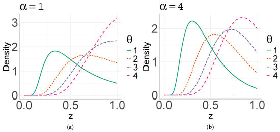
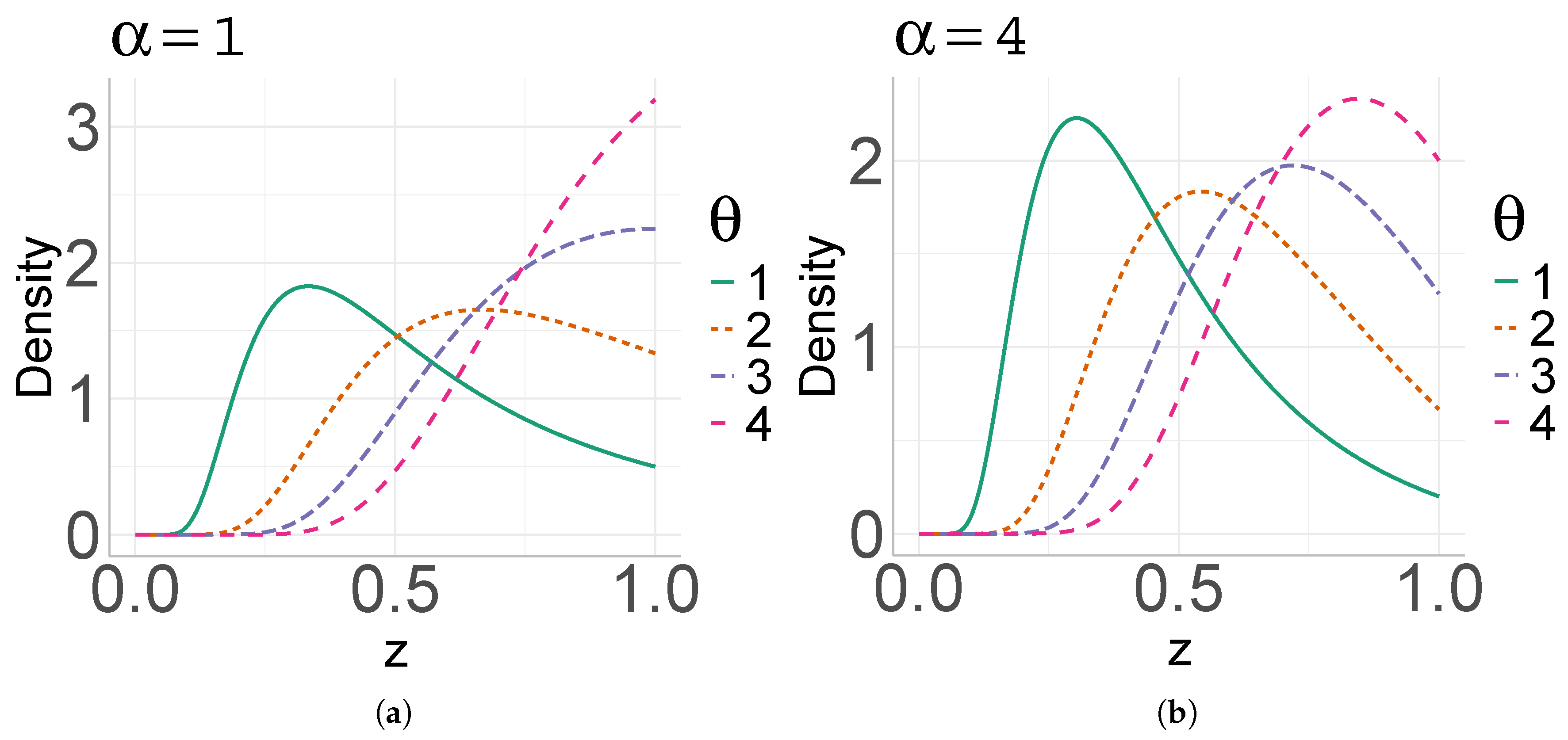
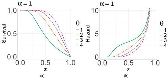
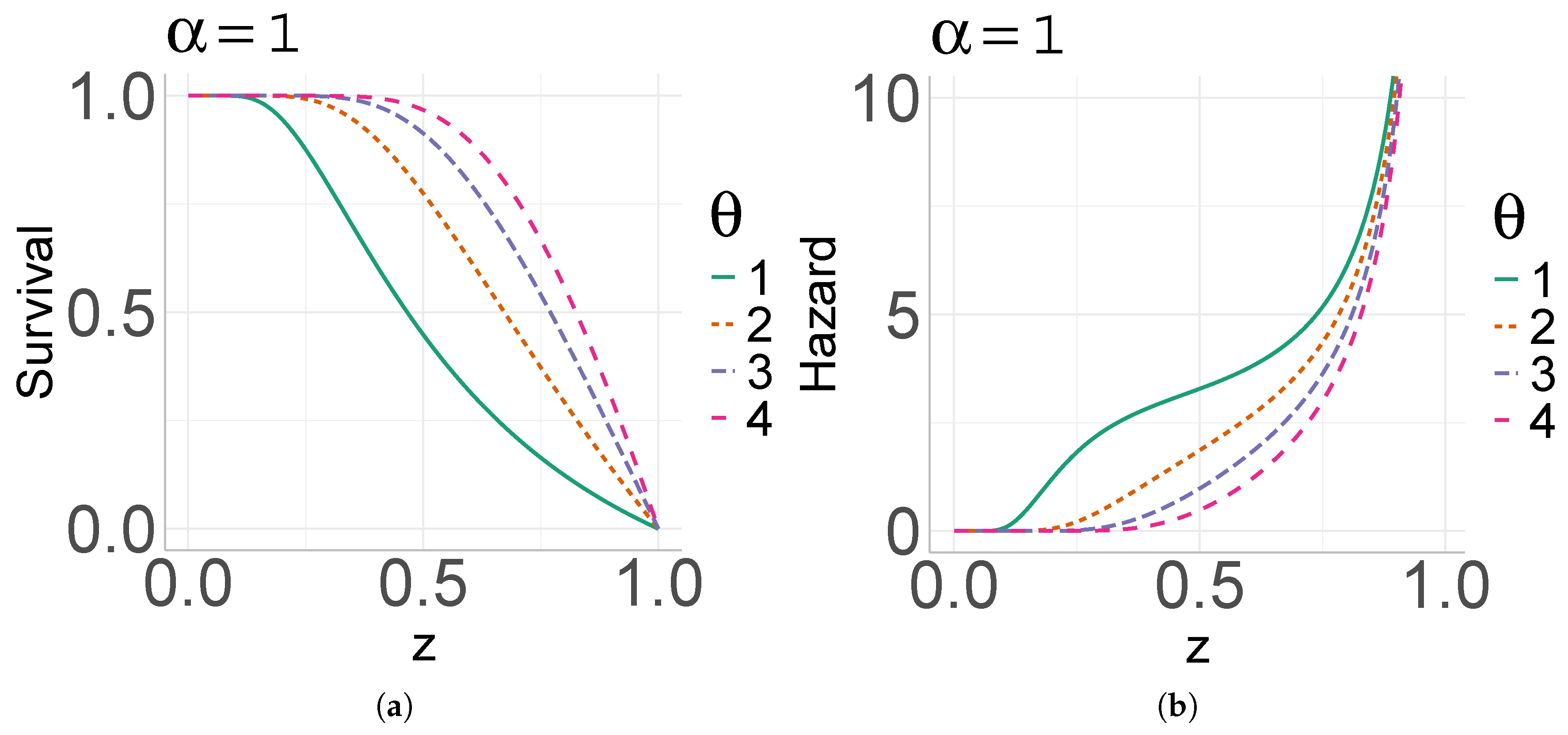
Figure 1 shows the pdf of the UEE distribution for $\alpha \in \{1,4\}$ and $\theta \in \{1,2,3,4\}$. Moreover, the sf and hf can be seen in Figure 2, where $\alpha$ is fixed at one.

Figure 1. The pdf of the UEE distribution, varying $\alpha$ and $\theta$. (a) $\alpha =1$, $\theta =1,2,3,4$. (b) $\alpha =4$, $\theta =1,2,3,4$.

Figure 2. (a) Survival function for $\alpha =1$ and $\theta =1,2,3,4$. (b) Hazard rate function for $\alpha =1$, $\theta =1,2,3,4$.

3.6. Order Statistics

Given a random sample of a size n from the $UEE(\theta ,\alpha )$, the jth order statistic is denoted by $Z_{\left(j\right)}$, with $1\le j\le n$.

Proposition 3.

The pdf of $Z_{\left(j\right)}$ is

$$\begin{array}{ccc}\hfill f_{Z_{\left(j\right)}}\left(z\right)& =& {\displaystyle \frac{n!{\theta }^2{e}^{\theta }(z+\alpha (1-z))}{(j-1)!(n-j)!{(\theta +\alpha )}^n}}{e}^{-{\displaystyle \frac{j\theta }{z}}+(j-1)\theta }{\left[\theta +{\displaystyle \frac{\theta \alpha }{z}}+\alpha -\alpha \theta \right]}^{j-1}\hfill \\ & \times & {\left[\theta +\alpha -e^{\theta -{\displaystyle \frac{\theta }{z}}}\left(\theta +{\displaystyle \frac{\theta \alpha }{z}}+\alpha -\alpha \theta \right)\right]}^{n-j},0<z<1.\hfill \end{array}$$

In particular, the pdf of the minimum, $Z_{\left(1\right)}$, is

$$f_{Z_{\left(1\right)}}\left(z\right)=n{\theta }^2{e}^{\theta }\left({\displaystyle \frac{z+\alpha (1-z)}{{(\theta +\alpha )}^n}}\right)e^{-{\displaystyle \frac{\theta }{z}}}{\left[\theta +\alpha -e^{\theta -{\displaystyle \frac{\theta }{z}}}\left(\theta +{\displaystyle \frac{\theta \alpha }{z}}+\alpha -\alpha \theta \right)\right]}^{n-1},0<z<1,$$

and the pdf of the maximum, $Z_{\left(n\right)}$, is

$$f_{Z_{\left(n\right)}}\left(z\right)=n{\theta }^2{e}^{\theta }\left({\displaystyle \frac{z+\alpha (1-z)}{{(\theta +\alpha )}^n}}\right)e^{-\theta ({\displaystyle \frac{n}{z}}-n+1)}{\left[\theta +{\displaystyle \frac{\theta \alpha }{z}}+\alpha -\alpha \theta \right]}^{n-1},0<z<1.$$

Proof. 

Since we are dealing with an absolutely continuous model, the pdf of the jth-order statistics is obtained by applying

$$\begin{array}{ccc}\hfill f_{Z_{\left(j\right)}}\left(z\right)& =& {\displaystyle \frac{n!}{(j-1)!(n-j)!}}f\left(z\right){\left[F\left(z\right)\right]}^{j-1}{[1-F\left(z\right)]}^{n-j},,j\in \{1,\dots ,n\}\hfill \end{array}$$

where F and f denote the cdf and pdf of the parent distribution, $Z\sim UEE(\theta ,\alpha )$, in this case, respectively.    □

3.7. Characterization Based on the Hazard Function

Characterizing a probability density function in terms of the hazard function is essential for understanding temporal event dynamics in diverse applications, such as reliability analysis. The following characterization is provided for the UEE distribution.

Theorem 1.

Let Z be a continuous random variable supported on $(0,1)$. Then, the probability density function of Z is given by Equation (9) if and only if its hazard rate function $h_Z\left(z\right)$ satisfies the following differential equation:

$$h_Z^{\prime }\left(z\right)-\left({\displaystyle \frac{1-\alpha }{z(1-\alpha )+\alpha }}-{\displaystyle \frac{3}{z}}+{\displaystyle \frac{\theta }{z^2}}\right)h_Z\left(z\right)=h_Z{\left(z\right)}^2.$$

(17)

Proof. 

The relationship between the density $f_Z\left(z\right)$ and the hazard function $h_Z\left(z\right)$ is known to be ${\displaystyle \frac{f_Z^{\prime }\left(z\right)}{f_Z\left(z\right)}}={\displaystyle \frac{h_Z^{\prime }\left(z\right)}{h_Z\left(z\right)}}-h_Z\left(z\right)$. Using the logarithmic derivative of the UEE density, we have

$${\displaystyle \frac{f_Z^{\prime }\left(z\right)}{f_Z\left(z\right)}}={\displaystyle \frac{1-\alpha }{z(1-\alpha )+\alpha }}-{\displaystyle \frac{3}{z}}+{\displaystyle \frac{\theta }{z^2}}.$$

Substituting this expression into the generic relationship yields Equation (17).    □

3.8. Moments

Proposition 4.

Let $Z\sim \mathrm{UEE}(\theta ,\alpha )$. Then, the rth moment is given by

$$E\left(Z^r\right)={\displaystyle \frac{{\theta }^2{e}^{\theta }}{\theta +\alpha }}\left[(1-\alpha )E_r\left(\theta \right)+\alpha E_{r-1}\left(\theta \right)\right],$$

(18)

where

$$E_r\left(\theta \right)={\int }_1^{\infty }{u}^{-r}{e}^{-\theta u}du.$$

(19)

Proof. 

To compute the moments, we use the definition $E\left(Z^r\right)={\int }_0^1{z}^r{f}_Z\left(z\right)dz$. By applying the transformation $u=1/z$, the limits of integration change from $(0,1)$ to $(\infty ,1)$, and the Jacobian is $dz=-u^{-2}du$. Thus, substituting the pdf of Z yields Equation (18).

The integral $E_r\left(\theta \right)$ can be analytically related to the upper incomplete gamma function, defined as $\Gamma (s,x)={\int }_x^{\infty }{t}^{s-1}{e}^{-t}dt$. By using the substitution $t=\theta u$, we obtain $E_r\left(\theta \right)={\theta }^{r-1}\Gamma (1-r,\theta )$. It is important to note that since the lower limit of integration is $\theta >0$, this integral avoids the singularity at the origin and converges absolutely for any $s=1-r\in \mathbb{R}$, ensuring that all positive moments are well defined. In the particular case where $r=1$, the second term involves $E_0\left(\theta \right)={\int }_1^{\infty }{e}^{-\theta u}du={\displaystyle \frac{1}{\theta }}{e}^{-\theta }$.    □

The function $E_r\left(\theta \right)$ facilitates direct numerical evaluation. In particular, the first two moments are given by

$$\begin{array}{cc}\hfill E\left(Z\right)& ={\displaystyle \frac{{\theta }^2{e}^{\theta }}{\theta +\alpha }}\left[(1-\alpha )E_1\left(\theta \right)+{\displaystyle \frac{\alpha }{\theta }}{e}^{-\theta }\right],\hfill \end{array}$$

(20)

$$\begin{array}{cc}\hfill E\left(Z^2\right)& ={\displaystyle \frac{{\theta }^2{e}^{\theta }}{\theta +\alpha }}\left[(1-\alpha )E_2\left(\theta \right)+\alpha E_1\left(\theta \right)\right].\hfill \end{array}$$

(21)

The variance follows as $\mathrm{Var}\left(Z\right)=E\left(Z^2\right)-{\left[E\left(Z\right)\right]}^2$. The skewness ($\sqrt{{\beta }_1}$) and kurtosis (${\beta }_2$) coefficients are given by

$${\displaystyle \sqrt{{\beta }_1}=\frac{W_3-3k{W}_1{W}_2+2k^2{W}_1^3}{\sqrt{k}{(W_2-k{W}_1^2)}^{3/2}},}$$

$${\displaystyle {\beta }_2=\frac{W_4-4k{W}_1{W}_3+6k^2{W}_1^2{W}_2-3k^3{W}_1^4}{k{(W_2-k{W}_1^2)}^2},}$$

where $k={\displaystyle \frac{{\theta }^2{e}^{\theta }}{\theta +\alpha }}$ and $W_i=(1-\alpha )E_1\left(\theta \right)+\alpha E_{i-1}\left(\theta \right)$, $i=1,2,3,4.$

All positive moments of the UEE distribution exist for $\theta >0$, since the integral $E_r\left(\theta \right)$ is finite for all $r\ge 1$. This ensures that the distribution is well defined for statistical inference purposes.

The following lemma is hepful to find the mean residual life function, denoted by $m\left(t\right)$.

Lemma 1.

For the special function introduced in Equation (19), we have

$$E_1\left(\theta \right)-E_1\left({\displaystyle \frac{\theta }{t}}\right)={\int }_1^{{\displaystyle \frac{1}{t}}}{u}^{-1}{e}^{-\theta u}du.$$

Proof. 

Using (19), we obtain

$$\begin{array}{ccc}\hfill E_1\left(\theta \right)-E_1\left({\displaystyle \frac{\theta }{t}}\right)& =& {\int }_1^{\infty }{u}^{-1}{e}^{-\theta u}du-{\int }_1^{\infty }{u}^{-1}{e}^{-{\displaystyle \frac{\theta u}{t}}}du\hfill \\ & =& {\int }_1^{{\displaystyle \frac{1}{t}}}{u}^{-1}{e}^{-\theta u}du+{\int }_{{\displaystyle \frac{1}{t}}}^{\infty }{u}^{-1}{e}^{-\theta u}du-{\int }_1^{\infty }{u}^{-1}{e}^{-{\displaystyle \frac{\theta u}{t}}}du,\hfill \end{array}$$

and making the change of variable $v={\displaystyle \frac{u}{t}}$ in the last integral yields the proposed result.    □

Recall that, by definition, the $m\left(t\right)$ of Z is given by

$$\begin{array}{c}\hfill m\left(t\right)=E(Z-t|Z>t)=E(Z|Z>t)-t.\end{array}$$

(22)

Next, we derive an expression for the mean residual life function, $m\left(t\right)$, of Z.

Proposition 5.

Let $Z\sim UEE(\theta ,\alpha )$. Then, the $m\left(t\right)$ of Z is given by

$$m\left(t\right)={\displaystyle \frac{\theta e^{-\theta }\left[\theta (1-\alpha )\left(E_1\left(\theta \right)-E_1\left(\frac{\theta }{t}\right)\right)-e^{-\frac{\theta }{t}}+e^{\theta }\right]}{\theta +\alpha -e^{\theta -\frac{\theta }{t}}\left(\theta +\frac{\theta \alpha }{t}+\alpha -\alpha \theta \right)}}-t.$$

Proof. 

For $Z\sim UEE(\theta ,\alpha )$, we have

$$E\left(Z\right|Z>t)={\displaystyle \frac{{\int }_t^{1}zf(z;\theta ,\alpha )dz}{R_Z(t;\theta ,\alpha )}},$$

and then, through ${\int }_t^{1}zf(z;\theta ,\alpha )dz={\int }_t^{1}z{\displaystyle \frac{{\theta }^2}{\theta +\alpha }}\left({\displaystyle \frac{z+\alpha (1-z)}{z^3}}\right)e^{\theta -{\displaystyle \frac{\theta }{z}}}dz={\displaystyle \frac{{\theta }^2{e}^{\theta }}{\theta +\alpha }}{\int }_t^1\left({\displaystyle \frac{z+\alpha (1-z)}{z^2}}{e}^{-{\displaystyle \frac{\theta }{z}}}\right)dz.$ By making the change in variable $u={\displaystyle \frac{1}{z}}$ and using Lemma 1 and Equation (22), the result is obtained.    □

4. Inference

This section introduces three estimation methods whose performance will be compared in Section 5.

Let $\mathit{z}=(z_1,\dots ,z_n)$ be a random sample from $UEE(\theta ,\alpha )$. Then, the likelihood function is

$$L(\theta ,\alpha )={\displaystyle \prod _{i=1}^n}{\displaystyle \frac{{\theta }^2{e}^{\theta }}{\theta +\alpha }}\left({\displaystyle \frac{z_i+\alpha (1-z_i)}{z_i^3}}\right)exp\left(-{\displaystyle \frac{\theta }{z_i}}\right).$$

(23)

4.1. Maximum Likelihood Estimation

To find the maximum likelihood estimators, it is typical to consider the log-likelihood function. Thus, by taking the natural logarithm of Equation (23) and using the properties of logarithms, the log-likelihood function, $\mathcal{\ell }(\theta ,\alpha )$, is

$$\begin{array}{cc}\hfill \mathcal{\ell }(\theta ,\alpha )& =2nlog\theta +n\theta -nlog(\theta +\alpha )\hfill \end{array}$$

(24)

$$\begin{array}{cc}\hfill & -\theta {\displaystyle \sum _{i=1}^n}{\displaystyle \frac{1}{z_i}}+{\displaystyle \sum _{i=1}^n}log\left(z_i+\alpha (1-z_i)\right)-3{\displaystyle \sum _{i=1}^n}log{z}_i.\hfill \end{array}$$

(25)

To find the stationary points that maximize Equation (24), we compute the first-order partial derivatives of $\mathcal{\ell }(\theta ,\alpha )$ with respect to each parameter and set them equal to zero. The following score equations are obtained:

$$\begin{array}{cc}\hfill {\displaystyle \frac{\partial \mathcal{\ell }}{\partial \theta }}& ={\displaystyle \frac{2n}{\theta }}+n-{\displaystyle \frac{n}{\theta +\alpha }}-{\displaystyle \sum _{i=1}^n}{\displaystyle \frac{1}{z_i}}=0,\hfill \end{array}$$

(26)

$$\begin{array}{cc}\hfill {\displaystyle \frac{\partial \mathcal{\ell }}{\partial \alpha }}& =-{\displaystyle \frac{n}{\theta +\alpha }}+{\displaystyle \sum _{i=1}^n}{\displaystyle \frac{1-z_i}{z_i+\alpha (1-z_i)}}=0.\hfill \end{array}$$

(27)

These score equations reveal that a closed-form solution for $\widehat{\theta }$ and $\widehat{\alpha }$ is not mathematically tractable. However, we can establish the existence and uniqueness of the maximum likelihood estimates through the following proposition.

Proposition 6.

Let $\mathit{z}=(z_1,\dots ,z_n)$ be a random sample from the $UEE(\theta ,\alpha )$ distribution. Then, the maximum likelihood estimates $(\widehat{\theta },\widehat{\alpha })$ exist and are unique.

Proof. 

We start by showing their existence. Let us fix $\alpha >0$ and analyze the score equation for $\theta$. If we define $g\left(\theta \right)={\displaystyle \frac{2n}{\theta }}+n-{\displaystyle \frac{n}{\theta +\alpha }}$, then its derivative with respect to $\theta$ is given by $g^{\prime }\left(\theta \right)=-{\displaystyle \frac{2n}{{\theta }^2}}+{\displaystyle \frac{n}{{(\theta +\alpha )}^2}}$. Notice that since $\alpha >0$, we have ${(\theta +\alpha )}^2>{\theta }^2$, which immediately implies $g^{\prime }\left(\theta \right)<0$. Thus, $g\left(\theta \right)$ is a strictly decreasing function.

When evaluating the limits, we find ${lim}_{\theta \to 0^{+}}g\left(\theta \right)=\infty$ and ${lim}_{\theta \to \infty }g\left(\theta \right)=n$. From Equation (26), we need to solve $g\left(\theta \right)={\sum }_{i=1}^n{\displaystyle \frac{1}{z_i}}$. Since the observations belong to the unit interval ($z_i\in (0,1)$), then ${\sum }_{i=1}^n{\displaystyle \frac{1}{z_i}}>n$. Therefore, under the intermediate value theorem, there exists a unique root $\theta \left(\alpha \right)>0$ that satisfies Equation (26) for any given $\alpha$.

Next, we replace $\theta$ by $\theta \left(\alpha \right)$ in Equation (27) and define the function $h\left(\alpha \right)={\sum }_{i=1}^n{\displaystyle \frac{1-z_i}{z_i+\alpha (1-z_i)}}-{\displaystyle \frac{n}{\theta \left(\alpha \right)+\alpha }}$. When studying the behavior of this function at the boundaries, we see that if $\alpha \to 0^{+}$, then the first term approaches ${\sum }_{i=1}^n{\displaystyle \frac{1-z_i}{z_i}}>0$, and thus $h\left(\alpha \right)$ is positive for sufficiently small values of $\alpha$. On the other hand, as $\alpha \to \infty$, the first term trends toward zero. Since $\theta \left(\alpha \right)$ remains positive, $h\left(\alpha \right)$ eventually becomes strictly negative. Under Bolzano’s theorem, there must be at least one root $\widehat{\alpha }>0$ such that $h\left(\widehat{\alpha }\right)=0$. Finally, the uniqueness of this root—and consequently of the pair $(\widehat{\theta },\widehat{\alpha })$—follows from the strict concavity of the log-likelihood surface in the neighborhood of the maximum, which is consistent with the negative definiteness of the observed Fisher information matrix.    □

Since no closed-form solution exists, the maximum likelihood estimators must be obtained numerically using iterative optimization methods such as the Newton–Raphson or quasi-Newton algorithms. The likelihood function may exhibit flat regions or multiple local maxima, particularly for small samples. Therefore, careful selection of the initial values and robust optimization routines are recommended to ensure convergence.

The observed Fisher information matrix is defined by

$$I(\theta ,\alpha )=-\left(\begin{array}{cc}{\displaystyle \frac{{\partial }^2\mathcal{\ell }}{\partial {\theta }^2}}& {\displaystyle \frac{{\partial }^2\mathcal{\ell }}{\partial \theta \partial \alpha }}\\ {\displaystyle \frac{{\partial }^2\mathcal{\ell }}{\partial \alpha \partial \theta }}& {\displaystyle \frac{{\partial }^2\mathcal{\ell }}{\partial {\alpha }^2}}\end{array}\right).$$

(28)

The second derivatives are given by

$${\displaystyle \frac{{\partial }^2\mathcal{\ell }}{\partial {\theta }^2}}=-{\displaystyle \frac{2n}{{\theta }^2}}+{\displaystyle \frac{n}{{(\theta +\alpha )}^2}},$$

(29)

$${\displaystyle \frac{{\partial }^2\mathcal{\ell }}{\partial \theta \partial \alpha }}={\displaystyle \frac{n}{{(\theta +\alpha )}^2}},$$

(30)

$${\displaystyle \frac{{\partial }^2\mathcal{\ell }}{\partial {\alpha }^2}}={\displaystyle \frac{n}{{(\theta +\alpha )}^2}}-{\displaystyle \sum _{i=1}^n}{\displaystyle \frac{{(1-z_i)}^2}{{\left(z_i+\alpha (1-z_i)\right)}^2}}.$$

(31)

Under standard regularity conditions, the maximum likelihood estimators are consistent and asymptotically normal. It is important to note that these conditions are strictly satisfied for the UEE distribution because its support, $(0,1)$, does not depend on the unknown parameters $\theta$ and $\alpha$, and the probability density function is sufficiently smooth with continuous derivatives. Specifically, $\sqrt{n}\left(\widehat{\mathit{\eta }}-\mathit{\eta }\right)\stackrel{d}{\to }N\left(0,I^{-1}\left(\mathit{\eta }\right)\right)$, where $\mathit{\eta }={(\theta ,\alpha )}^T$ and $\widehat{\mathit{\eta }}$ denotes the ML estimate of $\mathit{\eta }$. This result allows the construction of approximate confidence intervals and hypothesis testing using the observed Fisher information matrix.

4.2. Bayesian Inference

Under Bayesian inference, the parameter set $(\theta ,\alpha )$ is considered random, with some defined prior distribution $f(\theta ,\alpha )$. Hence, estimation can be computed by obtaining, for example, the mean of the marginal posterior distributions $f(\theta \mid \mathit{z})$ and $f(\alpha \mid \mathit{z})$, which is the posterior mean. However, obtaining such distributions is difficult in most cases. Thus, an algorithm such as the Gibbs sampler can be considered, using the full conditional distributions $f(\theta \mid \alpha ,\mathit{z})$ and $f(\alpha \mid \theta ,\mathit{z})$, which are easier to obtain. While such an algorithm can be implemented under the UEE model, it would lead to unknown conditional posterior distributions for $\theta$ and $\alpha$, forcing the procedure to use Metropolis–Hastings sub-steps, which would make it unstable.

Instead, we propose working under the EE model with the reparameterization $p=\alpha /(\theta +\alpha )$ to guarantee known conditional posterior distributions. This proposal modifies the mixture representation given in Equation (6) to

$$\begin{array}{ccc}\hfill f_X(x;\theta ,p)& =& (1-p)f_{Exp}(x;\theta )+p{f}_{Gamma}(x;2,\theta ),\hfill \end{array}$$

(32)

and implies that $\alpha =\theta p/(1-p)$. Since the algorithm will work with the random sample of $X_i\sim EE(\theta ,\alpha )$, every observation will be computed as $x_i=(1-z_i/z_i)$, where $z_i$ is the ith individual of the observed sample $Z_i\sim UEE(\theta ,\alpha )$. Moreover, taking advantage of the EE distribution being a mixture, a latent binary variable ${\delta }_i$ can be introduced to indicate from which part of the mixture $X_i$ came:

$$\begin{array}{c}\hfill {\delta }_i=\left\{\begin{array}{cc}0\hfill & \mathrm{if}{X}_i\sim Exp\left(\theta \right),\hfill \\ 1\hfill & \mathrm{if}{X}_i\sim Gamma(2,\theta ).\hfill \end{array}\right.\end{array}$$

(33)

Therefore, the pdf in Equation (32) can be written as follows:

$$\begin{array}{ccc}\hfill f_X(x\mid \theta ,p,{\delta }_i)& =& {\left(f_{Exp}(x;\theta )\right)}^{1-{\delta }_i}{\left(f_{Gamma}(x;2,\theta )\right)}^{{\delta }_i},\hfill \end{array}$$

and the distribution of ${\delta }_i$ is $f({\delta }_i\mid p)=p^{{\delta }_i}{(1-p)}^{1-{\delta }_i}$.

To guarantee conjugacy, Gamma and Beta distributions were considered to be prior to $\theta$ and p, respectively. Given the sample of $\mathit{x}$, the conditional posterior distribution of $\alpha$, p, and ${\delta }_i$ needs to be obtained, as it is shown in the following proposition.

Proposition 7.

Let $X_i\sim EE(\theta ,p)$, $i=1,\dots ,n$ and $\mathit{\delta }=({\delta }_1,\dots ,{\delta }_n)$, as defined in Equation (33). Considering the priors $\theta \sim Gamma(a_{\theta },b_{\theta })$ and $p\sim Beta(a_p,b_p)$, the conditional posteriors of $\theta ,p$, and ${\delta }_i$ are

$$\begin{array}{ccc}\hfill {\delta }_i\mid \theta ,p,\mathit{x}& \sim & Bern\left(q_i\right),i=1,\dots ,n\hfill \\ \hfill \theta \mid p,\mathit{x},\mathit{\delta }& \sim & Gamma\left(a_{\theta }+n+D,b_{\theta }+S\right)\hfill \\ \hfill p\mid \theta ,\mathit{x},\mathit{\delta }& \sim & Beta\left(a_p+D,b_p+n-D\right),\hfill \end{array}$$

(34)

where $Bern\left(q_i\right)$ denotes the Bernoulli distribution with the parameter $q_i=p\theta x_i/(1+p(\theta x_i-1))$, $D={\sum }_{i=1}^n{\delta }_i$, and $S={\sum }_{i=1}^n{x}_i$.

Proof. 

With regard to the conditional posterior of ${\delta }_i$, we have

$$\begin{array}{ccc}\hfill p({\delta }_i\mid \theta ,p,\mathit{x})& \propto & f\left({\delta }_i\right)f(x_i\mid \theta ,p,{\delta }_i)\hfill \\ & \propto & {\left(p{\theta }^2{x}_i{e}^{-\theta x_i}\right)}^{{\delta }_i}{\left((1-p)\theta e^{-\theta x_i}\right)}^{(1-{\delta }_i)},\hfill \end{array}$$

which is a Bernoulli distribution with unnormalized weights $w_1=p{\theta }^2{x}_i{e}^{-\theta x_i}$ and $w_2=(1-p)\theta e^{-\theta x_i}$. After normalizing the weights, the posterior distribution is obtained.

Now, note that

$$\begin{array}{ccc}\hfill f(\mathit{x}\mid \theta ,{\delta }_i)f(\mathit{\delta }\mid p)& =& {\displaystyle \prod _{i=1}^n}{\left(\theta e^{-\theta x_i}\right)}^{1-{\delta }_i}{\left({\theta }^2{x}_i{e}^{-\theta x_i}\right)}^{{\delta }_i}{p}^{{\delta }_i}{(1-p)}^{1-{\delta }_i}\hfill \\ & =& {\theta }^{n+{\sum }_{i=1}^n{\delta }_i}{e}^{-\theta {\sum }_{i=1}^n{x}_i}{x}_i^{{\sum }_{i=1}^n{\delta }_i}{p}^{{\sum }_{i=1}^n{\delta }_i}{(1-p)}^{n-{\sum }_{i=1}^n{\delta }_i}.\hfill \end{array}$$

Thus, the proposed conditional posterior distributions of $\alpha$ and p are obtained.    □

Finally, to apply these results in the UEE distribution, i.e., for a sample $z_1,\dots ,z_n$, with $Z_i\sim UEE(\theta ,\alpha )$, Algorithm 1 must be applied.

Algorithm 1 Gibbs sampling.

1: Make $x_i=(1-z_i)/z_i,i=1,\dots ,n$ Ensure: ${\theta }^{\left(0\right)}$, $p^{\left(0\right)}$, ${\mathit{\delta }}^{\left(0\right)}$                      ▹ Initial values For $t=1,\dots ,T$ do:                    ▹ Gibbs chain   2: Draw ${\delta }_i^{\left(t\right)}\mid {\theta }^{(t-1)},p^{(t-1)},\mathit{x}\sim Bern\left(q_i^{(t-1)}\right),i=1,\dots ,n$   ▹ See Equation (34)   3: Draw ${\theta }^{\left(t\right)}\mid p^{(t-1)},\mathit{x},{\mathit{\delta }}^{\left(t\right)}\sim Gamma\left(a_{\theta }+n+D,b_{\theta }+S\right)$    ▹ See Equation (34)   4: Draw $p^{\left(t\right)}\mid {\theta }^{\left(t\right)},\mathit{x},{\mathit{\delta }}^{\left(t\right)}\sim Beta\left(a_p+D,b_p+n-D\right)$           ▹ See Equation (34)   5: Make ${\alpha }^{\left(t\right)}={\theta }^{\left(t\right)}{p}^{\left(t\right)}/(1-p^{\left(t\right)})$ end for 6: Compute the estimators $\widehat{\theta }=(1/n){\sum }_{t=1}^T{\theta }^{\left(t\right)}$ and $\widehat{\alpha }=(1/n){\sum }_{t=1}^T{\alpha }^{\left(t\right)}$

4.3. Maximum Product of Spacing

The maximum product of spacing (MPS) method is a powerful alternative to MLEs for parameter estimation. The procedure was proposed in [7,8] as an approximation of the Kullback–Leibler information measure. Similar to the MLEs, this method returns estimators with properties such as invariance, consistency, and asymptotic efficiency. The uniform spacing for a random sample $Z_1,\dots ,Z_N$ is given by

$$\begin{array}{cc}\hfill D_i(\psi ;\mathit{z})=& F(z_{\left(i\right)}\mid \psi )-F(z_{(i-1)}\mid \psi ),i=1,2,\dots ,n+1,\hfill \end{array}$$

where $\psi =(\theta ,\alpha )$, $z_{\left(1\right)}<\dots <z_{\left(n\right)}$ are the order statistics, $F(z_{\left(0\right)}\mid \psi )=0$ and $F(z_{(n+1)}\mid \psi )=1.$ This implies that ${\sum }_{i=1}^{n+1}{D}_i(\psi ;\mathit{z})=1$.

The estimates for the parameters $\theta$ are obtained from the maximization of the geometric mean of uniform spaces

$$G\left(\psi ;\mathit{z}\right)={\left[{\displaystyle \prod _{i=1}^{n+1}}{D}_i(\psi ;\mathit{z})\right]}^{{\displaystyle \frac{1}{n+1}}}$$

in terms of $\psi$ or, equivalently, by maximizing its logarithm:

$$H\left(\psi ;\mathit{z}\right)={\displaystyle \frac{1}{n+1}}{\displaystyle \sum _{i=1}^{n+1}}log{D}_i(\theta ;\psi ).$$

5. Simulation Study

A Monte Carlo (MC) simulation study was conducted by using R software, version 4.5.3 [9] to evaluate the model’s ability to recover the true parameters $\theta$ and $\alpha$ under the ML, Bayesian, and MPS estimation methods. Algorithm 2 shows how to simulate values from the UEE distribution. A total of 16 scenarios were considered, combining different parameter values and sample sizes $n=200,500$ and 1000. The true parameter values varied under these scenarios.

Algorithm 2 Simulating $Z_i\sim UEE(\theta ,\alpha )$.

1: Fix $\alpha$, $\theta$, and compute $p=\theta /(\theta +\alpha )$ For $i=1,\dots ,n$ do:                     ▹ Sample size   2: Simulate $U_i\sim Unif(0,1)$              ▹ Uniform distribution   3: If $U_i\le p$, then simulate $X_i\sim Exp\left(\theta \right)$  ▹$\theta$: Rate parameter                      else, simulate $X_i\sim Gamma(2,\theta )$   4: Make $Z_i=1/(1+X_i)$ end for

For each scenario and sample size, $R=10,000$ experiments were conducted for the ML and MPS methods. The Bayesian method ran $R=1000$ experiments with a chain size of 10,000, a burn-in period of 2000, a hyperparameter $a_{\theta }=b_{\theta }=1$ and $a_p=b_p=2$ so that the prior for p was concentrated around $0.5$. While it is true that the Bayesian method has fewer experiments, it is usually expected to be balanced by the chain size. If not, then the problem is the chain size and not the number of experiments.

For each experiment with ML and Bayesian methods, the bias, root mean squared error (RMSE) and coverage probability (CP) of, for instance, $\theta$ were approximated using asymptotic normal $95\%$ confidence intervals. The bias and RMSE were computed as follows:

$$\begin{array}{c}\hfill {\mathrm{Bias}}_r={\displaystyle \frac{1}{R}}{\displaystyle \sum _{r=1}^n}({\widehat{\theta }}_r-\theta ),{\mathrm{RMSE}}_r=\sqrt{{\displaystyle \frac{1}{R}}\sum _{r=1}^n{({\widehat{\theta }}_r-\theta )}^2},\end{array}$$

where ${\widehat{\theta }}_r$ is the estimator of the corresponding estimation method of the rth experiment. Regarding the ML method, the standard error (SE) was computed by ${\mathrm{SE}}_r=\sqrt{\mathrm{diag}\left(I^{-1}({\widehat{\theta }}_r,{\widehat{\alpha }}_r)\right)}$. Meanwhile, in the Bayesian method, the standard deviation of the parameter chain $({\theta }_r^{\left(1\right)},{\theta }_r^{\left(T\right)})$ was computed as $S{E}_r$, where ${\theta }_r^{\left(t\right)}$ is the tth Gibbs sampler iteration of the rth experiment. Afterward, the mean of all ${\mathrm{Bias}}_r$, ${\mathrm{RMSE}}_r$, ${\mathrm{SE}}_r$ was given, namely $r=1,\dots ,R$, alongside the CP of the R experiments. These measures are not typically used to evaluate a Bayesian estimator, but they were computed nevertheless to make a fair comparison with the frequentist method.

Regarding the MPS method, the bias and RMSE are presented as the ML and Bayesian methods. However, the quantity shown as the SE for each scenario was computed as the standard deviation of all its ${\widehat{\theta }}_r$. Hence, the CP of the rth experiment uses that SE to obtain the confidence interval.

Table 1, Table 2 and Table 3 show the MC average of the previously introduced measurements for the ML, Bayesian and MPS methods, respectively. The results indicate that the UEE model’s performance improved consistently as the sample size increased. For different combinations of the parameter’s true values, the bias, RMSE and SE decreased and approached zero as the sample size increased. A similar behavior was observed for the CP, becoming more reliable as n increased, as can be seen in its approach to the nominal level of 0.95. Notably, the $\theta$ estimates were more stable across almost all scenarios, with small bias, RMSE and SE values and a CP close to 0.95. These results held especially for small values of the true value of $\theta$. In some experiments, larger values for the bias and SE for estimating $\alpha$ were obtained, implying larger means than for estimating $\theta$. Nevertheless, this effect was quite specific rather than systematic, and the magnitude of the bias, RMSE, and SE decreased as n increased.

Table 1. ML recovery parameter results for the simulation study of the UEE distribution.

Parameters			n = 200				n = 500				n = 1000
$\mathit{\theta }$	$\mathit{\alpha }$	Estimator	Bias	RMSE	SE	CP	Bias	RMSE	SE	CP	Bias	RMSE	SE	CP
1	1	$\alpha$	0.229	0.941	0.777	0.951	0.065	0.446	0.425	0.948	0.036	0.298	0.292	0.951
		$\theta$	0.001	0.112	0.113	0.954	−0.002	0.069	0.068	0.957	0.000	0.048	0.047	0.949
	2	$\alpha$	0.522	2.324	1.656	0.932	0.160	0.817	0.770	0.942	0.082	0.545	0.518	0.950
		$\theta$	0.003	0.085	0.084	0.954	0.001	0.053	0.053	0.952	0.001	0.037	0.037	0.951
	3	$\alpha$	1.129	4.579	3.547	0.924	0.325	1.447	1.265	0.939	0.135	0.840	0.809	0.946
		$\theta$	0.003	0.075	0.075	0.954	0.002	0.047	0.047	0.950	0.000	0.032	0.033	0.958
	4	$\alpha$	1.807	6.929	6.224	0.914	0.540	2.250	1.923	0.934	0.277	1.309	1.198	0.948
		$\theta$	0.001	0.070	0.071	0.953	0.001	0.045	0.045	0.950	0.002	0.032	0.031	0.947
2	1	$\alpha$	0.283	1.189	1.084	0.905	0.125	0.644	0.640	0.974	0.050	0.446	0.441	0.973
		$\theta$	−0.009	0.293	0.333	0.929	0.001	0.191	0.198	0.934	−0.005	0.140	0.140	0.956
	2	$\alpha$	0.449	1.758	1.540	0.955	0.169	0.907	0.861	0.951	0.079	0.603	0.586	0.950
		$\theta$	0.001	0.219	0.224	0.956	0.002	0.136	0.136	0.954	0.000	0.095	0.095	0.951
	3	$\alpha$	0.727	2.801	2.240	0.938	0.227	1.235	1.166	0.947	0.110	0.809	0.790	0.952
		$\theta$	0.006	0.187	0.187	0.956	0.001	0.116	0.115	0.953	0.002	0.081	0.081	0.950
	4	$\alpha$	1.042	3.990	3.171	0.934	0.294	1.614	1.529	0.944	0.156	1.060	1.032	0.953
		$\theta$	0.007	0.169	0.169	0.955	0.001	0.104	0.105	0.958	0.001	0.074	0.074	0.953
3	1	$\alpha$	0.466	1.621	1.492	0.876	0.165	0.889	0.902	0.903	0.059	0.627	0.638	0.933
		$\theta$	0.020	0.478	0.590	0.914	−0.013	0.347	0.393	0.923	−0.022	0.269	0.287	0.926
	2	$\alpha$	0.469	1.996	1.811	0.946	0.188	1.075	1.050	0.972	0.087	0.729	0.717	0.956
		$\theta$	−0.014	0.402	0.426	0.937	−0.003	0.249	0.254	0.956	−0.002	0.175	0.175	0.961
	3	$\alpha$	0.633	2.605	2.293	0.948	0.233	1.349	1.286	0.953	0.104	0.901	0.877	0.950
		$\theta$	−0.004	0.335	0.339	0.955	−0.002	0.203	0.204	0.957	−0.001	0.143	0.143	0.952
	4	$\alpha$	0.858	3.573	2.934	0.940	0.299	1.671	1.583	0.947	0.148	1.105	1.076	0.953
		$\theta$	0.001	0.295	0.295	0.958	0.002	0.182	0.181	0.952	0.001	0.127	0.127	0.952
4	1	$\alpha$	0.674	2.026	1.918	0.916	0.431	1.167	1.183	0.893	0.090	0.803	0.848	0.888
		$\theta$	0.079	0.661	0.854	0.916	0.095	0.461	0.531	0.836	−0.029	0.390	0.452	0.908
	2	$\alpha$	0.591	2.406	2.196	0.910	0.241	1.296	1.280	0.977	0.105	0.893	0.882	0.973
		$\theta$	−0.011	0.590	0.680	0.925	−0.003	0.375	0.397	0.941	−0.007	0.280	0.280	0.957
	3	$\alpha$	0.671	2.826	2.558	0.953	0.247	1.494	1.462	0.962	0.120	1.018	1.003	0.952
		$\theta$	−0.014	0.509	0.535	0.943	−0.003	0.315	0.314	0.959	−0.001	0.218	0.218	0.956
	4	$\alpha$	0.868	3.576	3.067	0.946	0.317	1.782	1.715	0.950	0.171	1.196	1.174	0.954
		$\theta$	0.002	0.450	0.450	0.952	0.003	0.272	0.272	0.957	0.003	0.188	0.189	0.955

Table 2. Bayesian recovery parameter results for the simulation study of the UEE distribution.

Parameters			n = 200				n = 500				n = 1000
$\mathit{\theta }$	$\mathit{\alpha }$	Estimator	Bias	RMSE	SE	CP	Bias	RMSE	SE	CP	Bias	RMSE	SE	CP
1	1	$\alpha$	0.187	0.779	0.759	0.957	0.045	0.409	0.423	0.953	0.037	0.300	0.294	0.958
		$\theta$	−0.020	0.091	0.102	0.969	−0.016	0.066	0.069	0.967	−0.005	0.049	0.048	0.950
	2	$\alpha$	0.207	1.342	1.511	0.923	0.087	0.730	0.767	0.944	0.066	0.521	0.519	0.952
		$\theta$	−0.027	0.081	0.086	0.962	−0.011	0.052	0.053	0.963	−0.004	0.035	0.037	0.971
	3	$\alpha$	0.279	2.113	2.810	0.911	0.176	1.336	1.285	0.923	0.083	0.830	0.812	0.944
		$\theta$	−0.031	0.079	0.077	0.941	−0.010	0.048	0.048	0.949	−0.005	0.034	0.033	0.946
	4	$\alpha$	0.507	3.089	4.821	0.907	0.225	1.904	1.956	0.932	0.111	1.187	1.181	0.948
		$\theta$	−0.028	0.074	0.072	0.947	−0.013	0.045	0.045	0.954	−0.005	0.031	0.032	0.955
2	1	$\alpha$	0.459	0.963	0.993	0.998	0.182	0.593	0.593	0.975	0.047	0.410	0.415	0.951
		$\theta$	0.026	0.192	0.227	0.978	−0.005	0.150	0.167	0.960	−0.024	0.123	0.129	0.949
	2	$\alpha$	0.270	1.332	1.444	0.959	0.083	0.828	0.846	0.947	0.031	0.558	0.579	0.961
		$\theta$	−0.052	0.187	0.205	0.966	−0.031	0.137	0.139	0.963	−0.019	0.097	0.096	0.949
	3	$\alpha$	0.241	2.003	2.091	0.918	0.065	1.123	1.143	0.937	0.031	0.786	0.782	0.935
		$\theta$	−0.066	0.189	0.187	0.952	−0.034	0.118	0.119	0.959	−0.014	0.084	0.082	0.947
	4	$\alpha$	0.212	2.426	2.823	0.917	0.206	1.708	1.562	0.930	0.038	1.006	1.016	0.932
		$\theta$	−0.075	0.179	0.172	0.944	−0.026	0.109	0.107	0.952	−0.015	0.076	0.075	0.952
3	1	$\alpha$	0.666	1.121	1.205	1.000	0.274	0.656	0.730	0.996	0.158	0.522	0.548	0.978
		$\theta$	0.072	0.279	0.349	0.987	0.019	0.211	0.262	0.974	0.003	0.184	0.213	0.968
	2	$\alpha$	0.468	1.581	1.647	0.978	0.072	0.901	0.979	0.954	0.018	0.696	0.702	0.949
		$\theta$	−0.059	0.282	0.327	0.971	−0.069	0.222	0.238	0.957	−0.044	0.177	0.177	0.949
	3	$\alpha$	0.236	1.935	2.085	0.940	0.046	1.256	1.251	0.935	−0.008	0.876	0.865	0.949
		$\theta$	−0.117	0.293	0.308	0.954	−0.062	0.212	0.210	0.950	−0.040	0.148	0.146	0.955
	4	$\alpha$	0.273	2.444	2.738	0.935	0.075	1.508	1.557	0.936	0.013	1.049	1.058	0.941
		$\theta$	−0.112	0.282	0.290	0.962	−0.055	0.192	0.187	0.948	−0.026	0.132	0.129	0.955
4	1	$\alpha$	1.004	1.512	1.491	1.000	0.448	0.802	0.886	0.999	0.243	0.604	0.654	0.990
		$\theta$	0.199	0.424	0.475	0.981	0.080	0.283	0.355	0.984	0.028	0.237	0.289	0.975
	2	$\alpha$	0.520	1.645	1.783	0.994	0.140	1.031	1.127	0.971	−0.003	0.776	0.824	0.955
		$\theta$	−0.076	0.361	0.447	0.975	−0.080	0.303	0.338	0.957	−0.074	0.254	0.265	0.953
	3	$\alpha$	0.428	2.090	2.304	0.963	−0.012	1.325	1.376	0.928	0.028	0.978	0.995	0.945
		$\theta$	−0.132	0.379	0.432	0.970	−0.120	0.312	0.311	0.939	−0.053	0.226	0.224	0.947
	4	$\alpha$	0.221	2.628	2.787	0.921	0.007	1.644	1.665	0.933	−0.020	1.142	1.154	0.953
		$\theta$	−0.170	0.407	0.414	0.944	−0.101	0.290	0.282	0.954	−0.052	0.197	0.196	0.960

Table 3. MPS recovery parameter results for the simulation study of the UEE distribution.

Parameters			n = 200				n = 500				n = 1000
$\mathit{\theta }$	$\mathit{\alpha }$	Estimator	Bias	RMSE	SE	CP	Bias	RMSE	SE	CP	Bias	RMSE	SE	CP
1	1	$\alpha$	−0.013	0.719	0.719	0.956	−0.017	0.432	0.431	0.952	−0.004	0.292	0.292	0.952
		$\theta$	−0.044	0.132	0.124	0.918	−0.016	0.072	0.071	0.943	−0.008	0.048	0.047	0.949
	2	$\alpha$	0.055	1.448	1.448	0.958	−0.005	0.710	0.710	0.954	0.035	0.557	0.556	0.949
		$\theta$	−0.029	0.093	0.089	0.940	−0.012	0.055	0.053	0.947	−0.005	0.039	0.039	0.943
	3	$\alpha$	0.345	3.584	3.569	0.982	−0.029	1.138	1.138	0.961	0.034	0.805	0.804	0.956
		$\theta$	−0.019	0.075	0.073	0.941	−0.013	0.050	0.048	0.944	−0.004	0.033	0.032	0.948
	4	$\alpha$	0.617	5.561	5.530	0.983	0.108	1.714	1.711	0.955	0.029	1.117	1.117	0.953
		$\theta$	−0.019	0.071	0.068	0.941	−0.008	0.045	0.044	0.945	−0.006	0.032	0.032	0.950
2	1	$\alpha$	−0.038	0.978	0.978	0.963	−0.081	0.633	0.628	0.965	−0.064	0.452	0.448	0.940
		$\theta$	−0.124	0.330	0.306	0.954	−0.079	0.229	0.215	0.898	−0.046	0.160	0.153	0.938
	2	$\alpha$	0.040	1.390	1.390	0.952	−0.074	0.823	0.820	0.956	−0.035	0.579	0.578	0.952
		$\theta$	−0.071	0.251	0.241	0.931	−0.042	0.147	0.141	0.946	−0.019	0.102	0.100	0.944
	3	$\alpha$	0.004	1.860	1.861	0.952	−0.005	1.087	1.087	0.954	−0.034	0.782	0.782	0.956
		$\theta$	−0.062	0.208	0.199	0.944	−0.031	0.117	0.113	0.954	−0.013	0.087	0.086	0.947
	4	$\alpha$	0.553	4.417	4.384	0.976	0.127	1.611	1.606	0.956	−0.054	1.038	1.037	0.956
		$\theta$	−0.042	0.183	0.178	0.946	−0.020	0.107	0.106	0.946	−0.014	0.078	0.077	0.960
3	1	$\alpha$	−0.042	1.277	1.277	0.967	−0.081	0.810	0.806	0.955	−0.065	0.640	0.637	0.973
		$\theta$	−0.186	0.501	0.465	0.977	−0.125	0.368	0.346	0.960	−0.088	0.306	0.293	0.906
	2	$\alpha$	−0.029	1.784	1.785	0.964	−0.074	1.026	1.024	0.962	−0.021	0.712	0.712	0.957
		$\theta$	−0.170	0.461	0.429	0.904	−0.084	0.290	0.278	0.929	−0.033	0.182	0.179	0.954
	3	$\alpha$	−0.132	2.006	2.002	0.961	−0.059	1.324	1.324	0.954	−0.009	0.902	0.903	0.957
		$\theta$	−0.138	0.386	0.361	0.921	−0.055	0.226	0.219	0.951	−0.026	0.149	0.147	0.950
	4	$\alpha$	−0.021	2.868	2.870	0.960	0.033	1.548	1.549	0.957	−0.009	1.071	1.072	0.948
		$\theta$	−0.113	0.335	0.315	0.933	−0.036	0.188	0.185	0.946	−0.022	0.132	0.131	0.949
4	1	$\alpha$	0.139	1.535	1.529	0.939	−0.032	0.999	0.999	0.953	−0.109	0.787	0.780	0.965
		$\theta$	−0.155	0.643	0.625	0.970	−0.155	0.506	0.482	0.980	−0.146	0.433	0.408	0.969
	2	$\alpha$	−0.062	2.108	2.108	0.958	−0.139	1.277	1.270	0.965	−0.079	0.912	0.909	0.951
		$\theta$	−0.240	0.661	0.616	0.959	−0.143	0.469	0.447	0.896	−0.082	0.312	0.301	0.939
	3	$\alpha$	−0.095	2.393	2.393	0.960	−0.118	1.476	1.472	0.939	−0.102	0.943	0.938	0.950
		$\theta$	−0.218	0.597	0.556	0.895	−0.108	0.370	0.354	0.941	−0.057	0.227	0.219	0.946
	4	$\alpha$	−0.007	3.008	3.009	0.963	0.006	1.692	1.692	0.966	−0.122	1.134	1.128	0.949
		$\theta$	−0.172	0.523	0.494	0.928	−0.062	0.287	0.280	0.952	−0.045	0.199	0.194	0.943

Overall, the three methods provided evidence of good performance for the proposed estimation procedure, with the best behavior observed for n = 1000, as expected. In particular, the MPS method achieved lower bias for $\alpha$ (especially for small n values) but maintained a similar RMSE and SE. On the other hand, the Bayesian method performed well when the true values of $\theta$ and $\alpha$ were similar but at the cost of longer estimation times due to the presence of the latent variable.

6. Applications

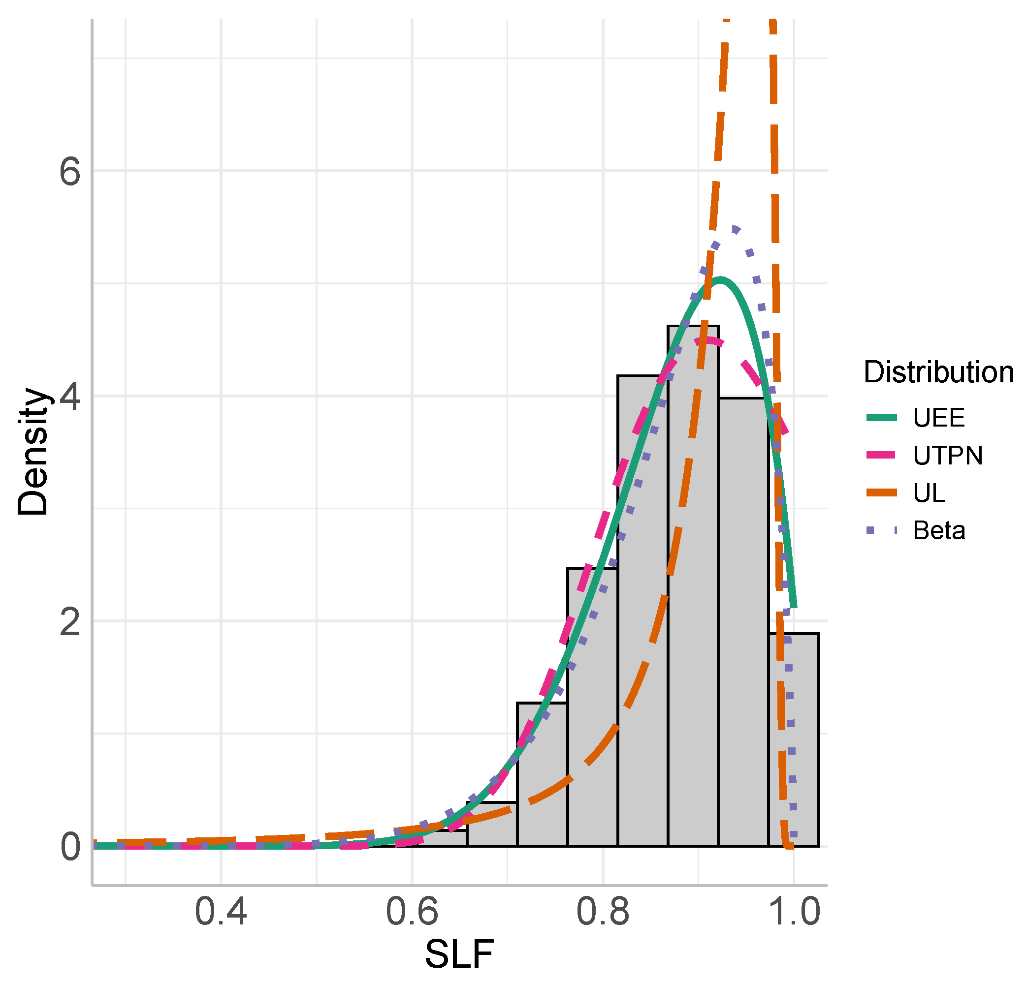
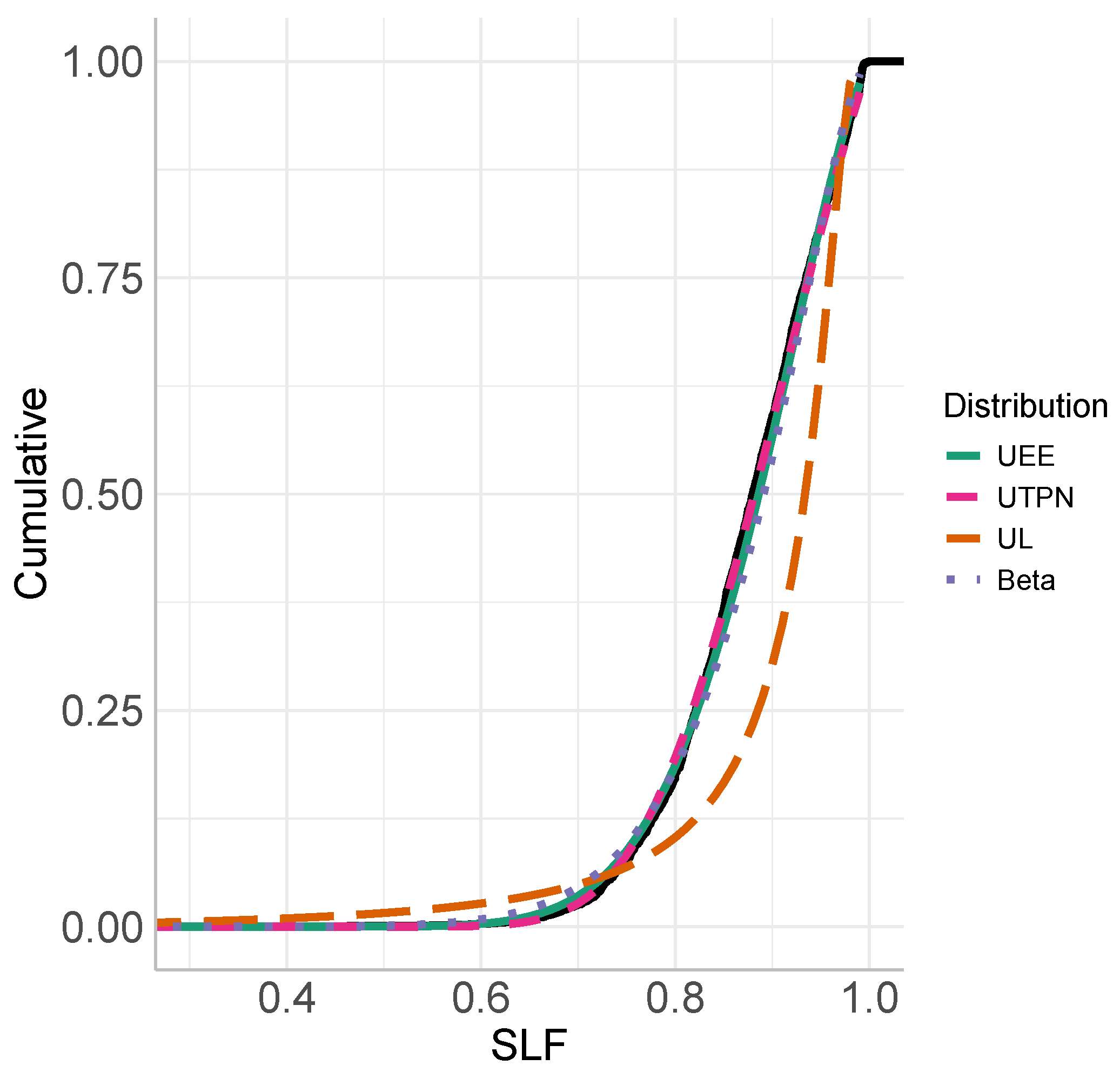
To illustrate our model applicability, we fitted two real data sets on the interval $(0,1)$. Our proposal was compared with the unit truncated positive normal (UTPN) [10], unit-Lindley $\left(\theta \right)$ and Beta $\left(\theta \right)$ distributions. We present the maximum likelihood (ml) parameter estimates with their standard errors in parentheses, along with the estimated log-likelihood. To measure the fitness of the models, the Akaike (see [11,12]) and Bayesian [13] information criteria were computed (AIC and BIC, respectively) alongside the p value of the Anderson–Darling normality test [14] on the quantile residuals. For the data, the estimated pdf and cdf under the three models are also shown, alongside their QQ plots.

6.1. Lung Function Data Set

The spirometric lung function (SLF) is the most common index for diagnosing pulmonary diseases (see, for instance, [15]). To obtain such an index, the FVC and FEV1 were first obtained. The FVC measures the amount of air that can be exhaled after taking the deepest possible breath. The FEV1 measures the same thing but in the first second of the FVC. Thus, the SLF is obtained as the quotient of the FEV1 and FVC; that is, $SLF=FEV1/FVC$. Clearly, the response variable has a range $(0,1)$, making our proposal suitable.

The data set used in this subsection, which can be extracted from the gamlss package lungFunction, consists of 3164 male observations of lung function. This study was previously analyzed in [16,17].

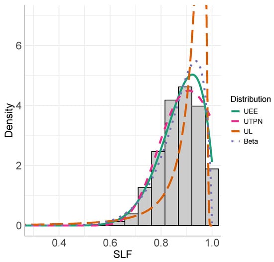
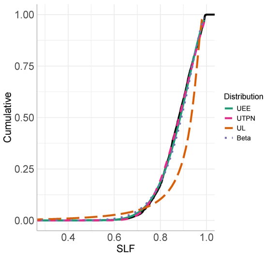
Table 4 shows the estimation results, while Figure 3 and Figure 4 present the estimated PDF and CDF on the data for the three models, respectively. The QQ plot is depicted in Figure 5. Despite the p value of the Anderson–Darling test, the AIC and BIC of the UEE distribution were lower than the other ones, as corroborated by the estimated PDF, the CDF fitted to the data and the QQ plot, which show a better fit than its competitors. Therefore, our proposal showed good performance in modeling sensitive data, such as lung capacity, a context that requires careful handling.

Table 4. ML estimates with their SE in parentheses, log-likelihood, AIC and BIC of the UEE, UTPN, UL and Beta distribution for the spirometric lung function data set.

	UEE	UTPN	UL	Beta
$\alpha$	52.07 (8.48)	0.57 (0.06)	- - - (- - -)	12.15 (0.34)
$\theta$	11.58 (0.21)	0.14 (<0.01)	0.11 (<0.01)	1.76 (0.04)
Log-likelihood	3393.48	3390.60	1768.57	3357.03
AIC	−6782.96	−6777.20	−3535.15	−6710.05
BIC	−6771.06	−3529.19	−6765.30	−6698.15
p value	<0.01	<0.01	<0.01	<0.01

Figure 3. Estimated PDF of the UEE (solid), UTPN (dashed), UL (longdash) and Beta (dotted) distribution on the spirometric lung function data set.

Figure 4. Estimated CDF of the UEE (solid), UTPN (dashed), UL (longdash) and Beta (dotted) distribution on the spirometric lung function data set.

Figure 5. QQ plot of the UEE, UTPN, UL and Beta distribution on the spirometric lung function data set.

6.2. Anxiety Data Set

This data set contains information about 166 women in Townsville, where their stress and anxiety among nonclinical individuals were observed. In particular, we focused on the anxiety variable, assessed using the Depression Anxiety Stress Scales, with a range of $(0,42)$. The authors of [18] transformed the variable into the interval $(0,1)$, making it suitable for our proposal.

No details about such a transformation were explicitly given. However, the used formulas can be inferred, thanks to their first mentioned data set. Let $x_i$ be a non-transformed data set (for example, $x_i\in (0,42)$ ). Then, the following transformation may have been used:

$$\begin{array}{ccc}\hfill Z_i^{\prime }& =& {\displaystyle \frac{x_i-a}{b-a}}\hfill \\ \hfill Z_i& =& {\displaystyle \frac{Z_i^{\prime }(n-1)+1/2}{n}},\hfill \end{array}$$

where $Z_i$ is the unit interval transformed data set, a and b are the minimum and maximum of the sample, respectively, and n is the sample size. The second line is to avoid entries of zeros and ones. The post-transformed data set can be loaded from the betareg package and StressAnxiety data.

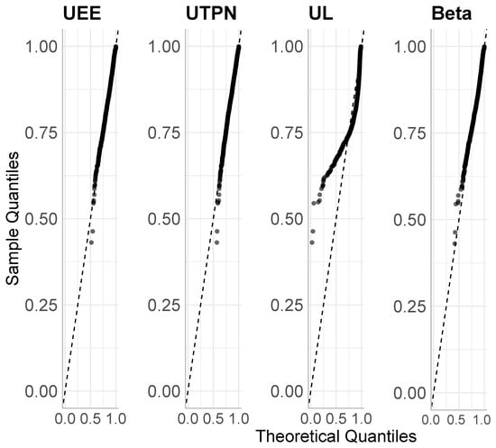
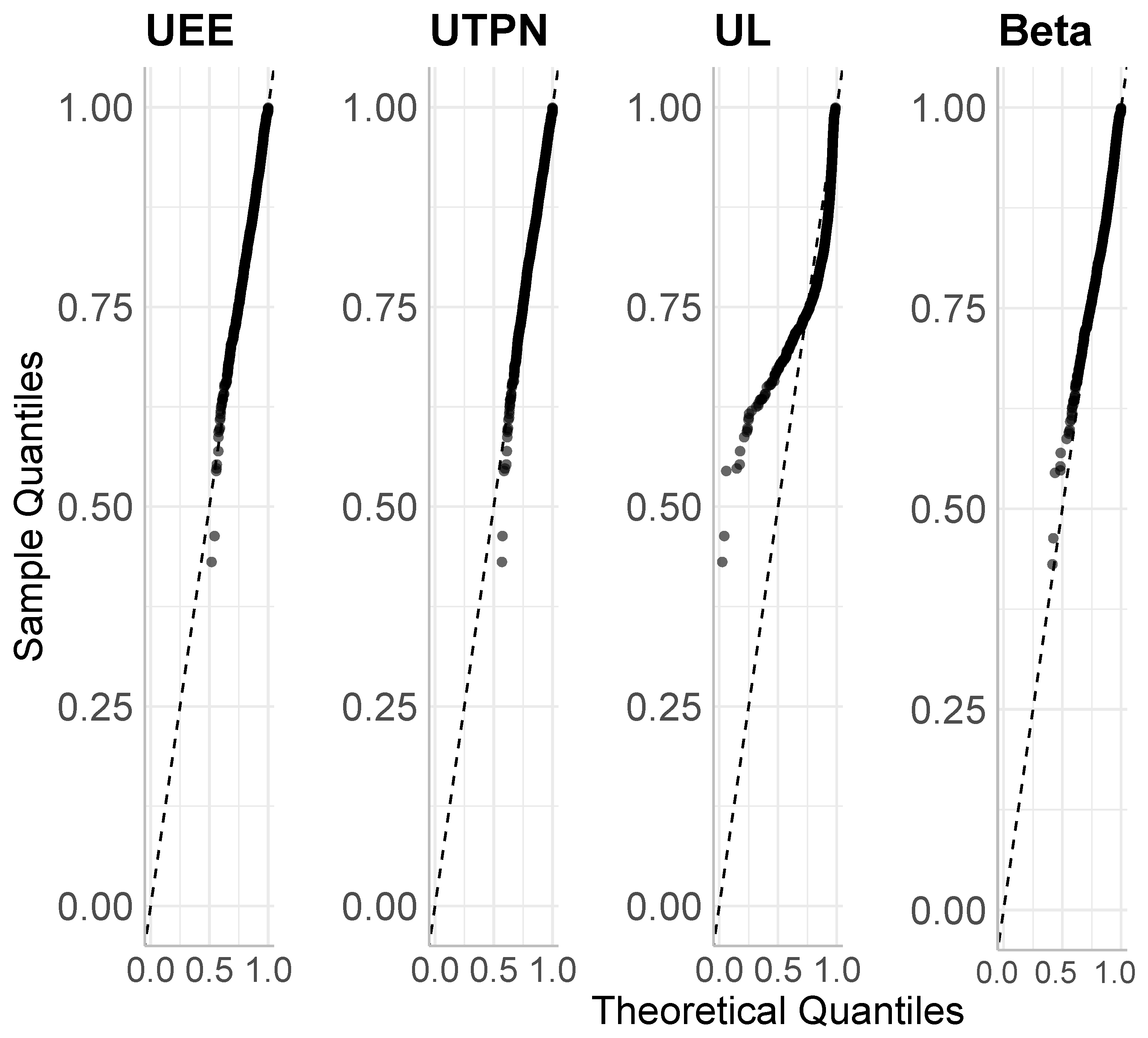
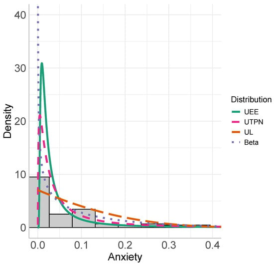
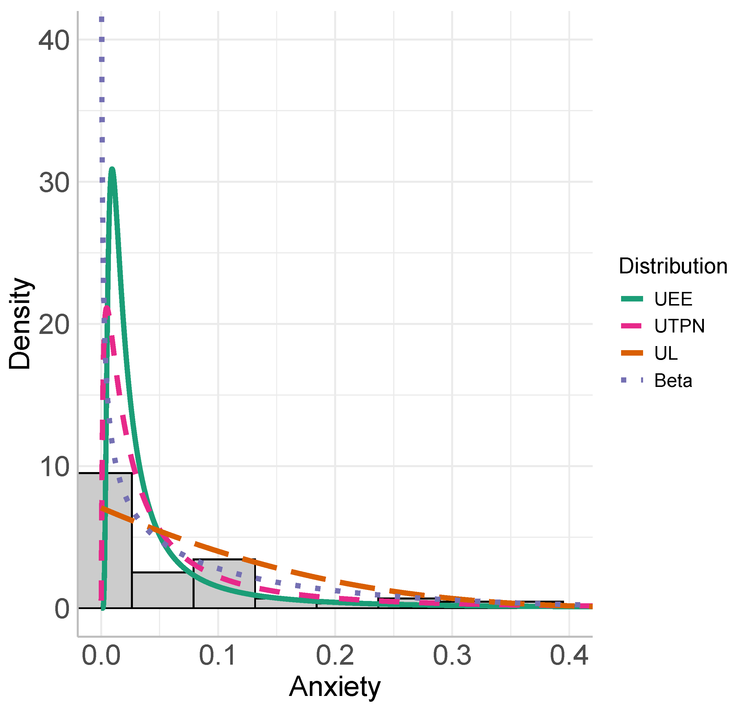
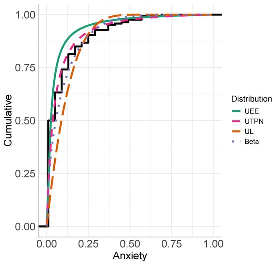
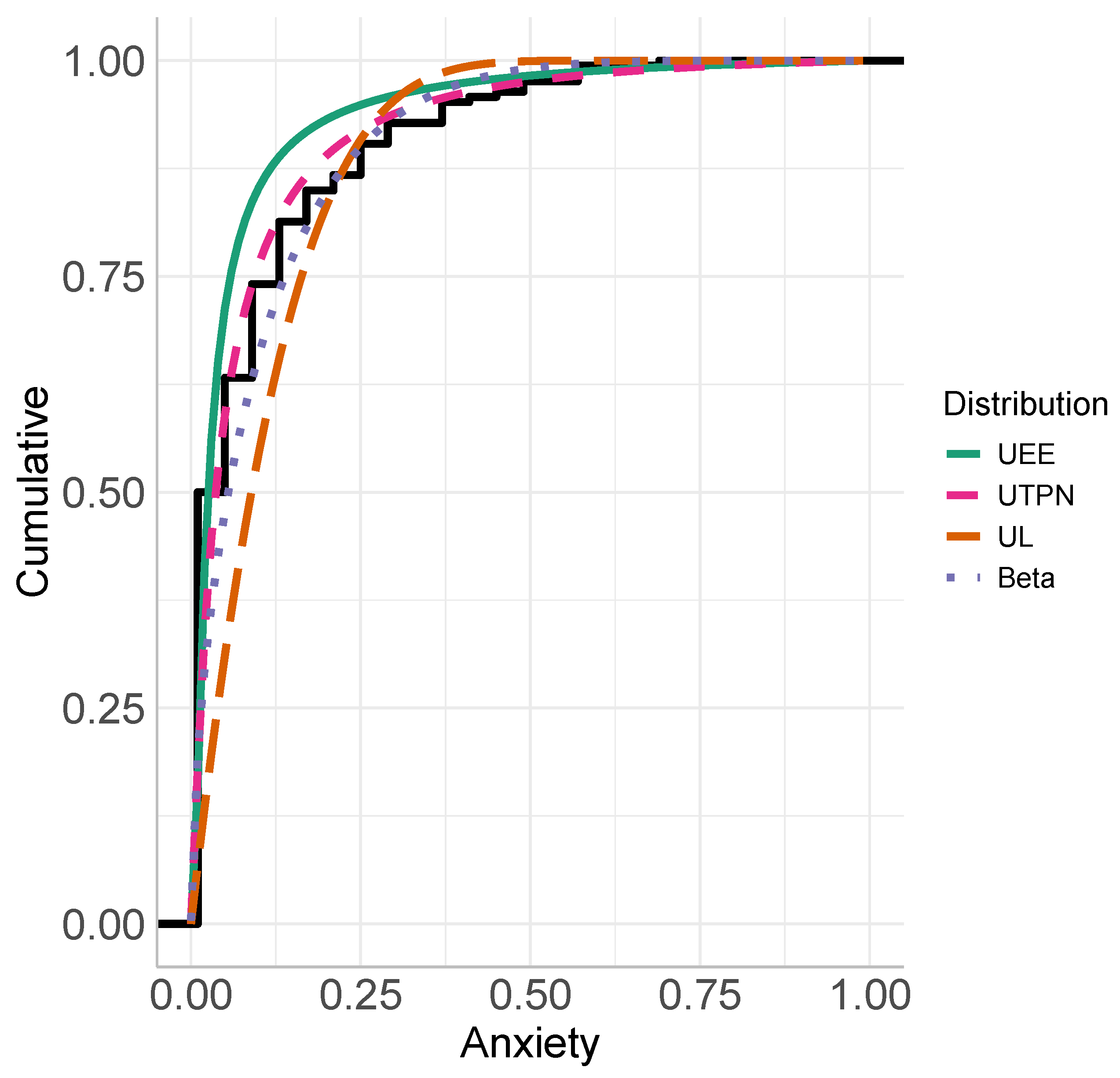
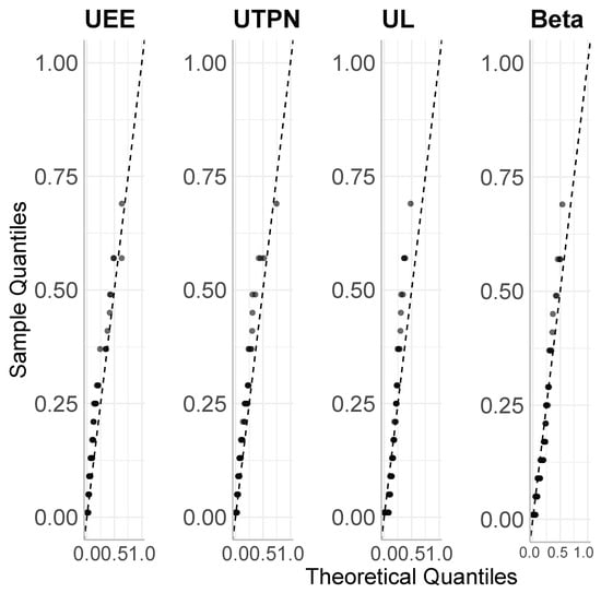
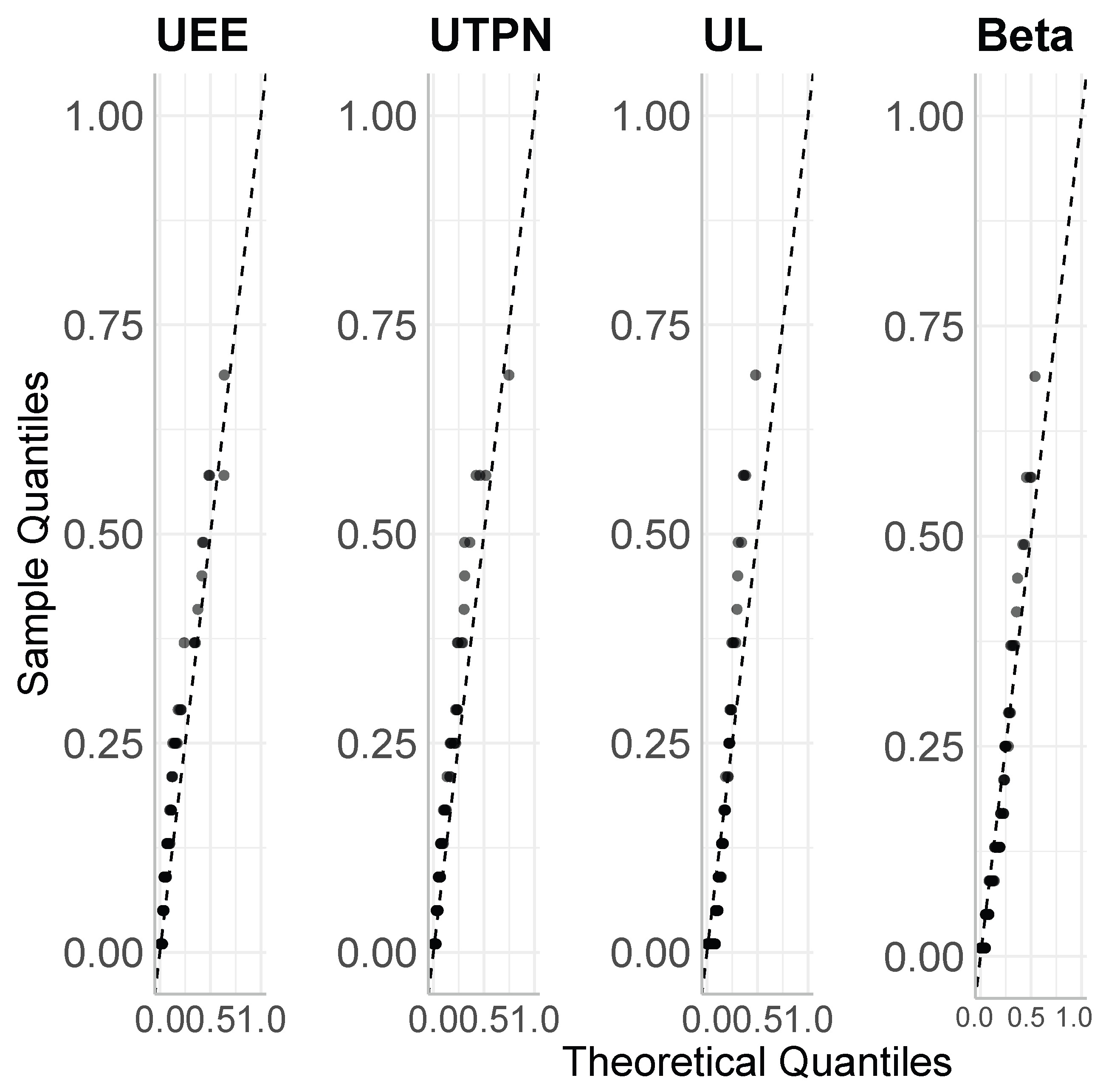
The estimation results are presented in Table 5. On the other hand, the estimated PDF, CDF and QQ plots for the UEE, UTPN, UL and Beta distributions are given in Figure 6, Figure 7 and Figure 8. Our distribution performed better than its competitor, as evidenced by its lower AIC and BIC, despite the presented p values. Therefore, our proposal represents a competitive alternative for unitary data sets, even when the data are concentrated around zero.

Table 5. ML estimates with their SE in parentheses, log-likelihood, AIC and BIC of the UEE, UTPN, UL and Beta distribution for the anxiety data set.

	UEE	UTPN	UL	Beta
$\alpha$	0.01 (0.01)	2.31 (0.18)	- - - (- - -)	0.58 (0.05)
$\theta$	0.02 (<0.01)	1.43 (0.09)	7.95 (0.56)	5.45 (0.71)
Log-likelihood	279.36	266.11	194.74	239.45
AIC	−554.72	−528.22	−387.48	−474.9
BIC	−548.5	−521.99	−384.36	−468.67
p-value	<0.01	<0.01	<0.01	<0.01

Figure 6. Estimated PDF of the UEE (solid), UTPN (dashed), UL (longdash) and Beta (dotted) distribution on the anxiety data set.

Figure 7. Estimated CDF of the UEE (solid), UTPN (dashed), UL (longdash) and Beta (dotted) distribution on the anxiety data set.

Figure 8. QQ plot of the UEE, UTPN, UL and Beta distribution on the anxiety data set.

7. Conclusions

In this paper, we introduced the UEE distribution, a novel probability model defined on the bounded interval $(0,1)$. Motivated by the inherent limitations of traditional models—such as the computational drawbacks of the Beta distribution when handling highly skewed proportional data—the UEE was developed via an algebraic transformation of the extended exponential distribution. This approach successfully maps a versatile, mixture-based baseline structure into the unit interval, yielding a highly flexible framework capable of accommodating severe asymmetries and boundary concentrations.

A comprehensive analytical study of the proposed model was carried out to establish its theoretical foundations. We derived explicit or computationally tractable expressions for its fundamental properties, including the probability density function, cumulative distribution, mode, quantile function and moments. Furthermore, we provided a mathematical characterization based on its hazard rate function, which sheds light on the structural dynamics of the distribution. Parameter estimation was rigorously addressed using the maximum likelihood framework, with asymptotic properties confirming the consistency and normality of the estimators. Bayesian techniques along with the maximum product of spacing estimation method were also considered.

The practical viability and empirical superiority of the proposed model were validated through extensive Monte Carlo simulations and real-world data analysis. The simulation study showed the robustness, low bias and finite-sample efficiency of the estimation methods across various sample sizes and parameter settings. Crucially, when applied to a highly skewed dataset on the unit interval, such as those provided in the applications, the UEE distribution consistently outperformed well-established classical alternatives, such as the unit-Lindley and Beta distributions, providing significantly better goodness of fit, as measured by standard information criteria (AIC and BIC).

Looking ahead, the analytical tractability and competitive performance of the UEE distribution open several promising avenues for future research. Immediate extensions include the formulation of bounded regression models linking the distribution’s parameters to external covariates, which would be highly valuable for applied econometrics and biostatistics. Additionally, exploring Bayesian inference paradigms to handle complex parameter spaces, as well as developing transmuted or generalized classes of the UEE model, represent natural and compelling progressions of this work.

References

- Johnson, N.L.; Kotz, S.; Balakrishnan, N. Continuous Univariate Distributions, 2nd ed.; John Wiley & Sons: New York, NY, USA, 1995; Volume 2. [Google Scholar]
- Kumaraswamy, P. A generalized probability density function for double-bounded random processes. J. Hydrol. 1980, 46, 79–88. [Google Scholar] [CrossRef] [Scilit]
- Mazucheli, J.; Menezes, A.F.B.; Chakraborty, S. On the one parameter unit-Lindley distribution and its associated regression model for proportion data. J. Appl. Stat. 2019, 46, 700–714. [Google Scholar] [CrossRef] [Scilit]
- Mazucheli, J.; Menezes, A.; Ghitany, M. The unit-Weibull distribution and associated inference. J. Appl. Probab. Stat. 2018, 13, 1–22. [Google Scholar]
- Menezes, A.; Mazucheli, J.; Dey, S. The unit-Logistic Distribution: Different Methods of Estimation. Pesqui. Oper. 2018, 38, 555–578. [Google Scholar] [CrossRef] [Scilit]
- Gómez, Y.; Bolfarine, H.; Gómez Geraldo, H. A New Extension of the Exponential Distribution. Rev. Colomb. EstadíStica 2014, 37, 25. [Google Scholar] [CrossRef] [Scilit]
- Cheng, R.; Amin, N. Estimating parameters in continuous univariate distributions with a shifted origin. J. R. Stat. Soc. Ser. Methodol. 1983, 45, 394–403. [Google Scholar] [CrossRef] [Scilit]
- Ranneby, B. The maximum spacing method. An estimation method related to the maximum likelihood method. Scand. J. Stat. 1984, 45, 93–112. [Google Scholar]
- R Core Team. R: A Language and Environment for Statistical Computing; R Foundation for Statistical Computing: Vienna, Austria, 2025. [Google Scholar]
- Salinas, H.S.; Bakouch, H.S.; Almuhayfith, F.E.; Caimanque, W.E.; Barrios-Blanco, L.; Albalawi, O. Statistical Advancement of a Flexible Unitary Distribution and Its Applications. Axioms 2024, 13, 397. [Google Scholar] [CrossRef] [Scilit]
- Akaike, H. Information Theory and an Extension of the Maximum Likelihood Principle. In Proceedings of the Second International Symposium on Information Theory; Akademiai Kiado: Budapest, Hungary, 1973; pp. 267–281. [Google Scholar]
- Akaike, H. A New Look at the Statistical Model Identification. IEEE Trans. Autom. Control. 1974, 19, 716–723. [Google Scholar] [CrossRef] [Scilit]
- Schwarz, G. Estimating the Dimension of a Model. Ann. Stat. 1978, 6, 461–464. [Google Scholar] [CrossRef] [Scilit]
- Anderson, T.W.; Darling, D.A. A Test of Goodness of Fit. J. Am. Stat. Assoc. 1954, 49, 765–769. [Google Scholar] [CrossRef]
- Quanjer, P.; Stanojevic, S.; Stocks, J.; Hall, G.; Prasad, K.; Cole, T.; Rosenthal, M.; Perez-Padilla, R.; Hankinson, J.; Falaschetti, E.; et al. Changes in the FEV1/FVC ratio during childhood and adolescence: An intercontinental study. Eur. Respir. J. 2010, 36, 1391–1399. [Google Scholar] [CrossRef] [Scilit] [PubMed]
- Stanojevic, S.; Wade, A.; Stocks, J.; Hankinson, J.; Coates, A.; Pan, H.; Rosenthal, M.; Corey, M.; Lebecque, P.; Cole, T. Reference Ranges for Spirometry Across All Ages. Am. J. Respir. Crit. Care Med. 2008, 177, 253–260. [Google Scholar] [CrossRef] [Scilit] [PubMed]
- Hossain, A.; Rigby, R.; Stasinopoulos, M.; Enea, M. Centile estimation for a proportion response variable. Stat. Med. 2016, 35, 895–904. [Google Scholar] [PubMed]
- Smithson, M.; Verkuilen, J. A better lemon squeezer? Maximum-likelihood regression with beta-distributed dependent variables. Psychol. Methods 2006, 11, 54–71. [Google Scholar] [CrossRef] [Scilit] [PubMed]
Disclaimer/Publisher’s Note: The statements, opinions and data contained in all publications are solely those of the individual author(s) and contributor(s) and not of MDPI and/or the editor(s). MDPI and/or the editor(s) disclaim responsibility for any injury to people or property resulting from any ideas, methods, instructions or products referred to in the content. |
© 2026 by the authors. Licensee MDPI, Basel, Switzerland. This article is an open access article distributed under the terms and conditions of the Creative Commons Attribution (CC BY) license.