Algebraically Stabilizing Blocks for Quantized and Finite-Precision Neural Networks

Abstract

This paper proposes a construction of algebraically stabilizing blocks for quantized and finite-precision neural networks. The approach is based on linear transformations defined by integer-valued matrices satisfying a condition of the form $W^k=I+\mu D$, which specifies algebraically controlled $k$-step behavior and modular periodicity in the integer-valued setting. The proposed property is invariant under conjugation, allowing the stabilizing construction to be transferred across equivalent linear representations. The resulting module can be integrated locally into existing neural architectures without requiring the algebraic structure to be imposed globally. The theoretical results concern algebraic and modular stabilization of the linear block and do not constitute a general guarantee of classical spectral or asymptotic stability in real-valued space. The approach is evaluated experimentally under multi-component harmonic, impulsive, and noisy inputs in both floating-point and INT8-quantized settings. Across several experimental configurations, the proposed block reduces output energy, component-wise variation, selected amplitude-related measures, and finite-precision deviation relative to floating-point reference trajectories. Norm-matched control experiments further suggest that the observed effects are not attributable solely to a reduction in operator magnitude, but may also reflect structural properties of the algebraically constructed operator. The proposed construction is particularly relevant to neural systems operating under limited numerical precision, including FPGA-, ASIC-, and edge-oriented implementations. It provides a structural approach for incorporating formally specified algebraic properties into the design of neural-network architectures.

1. Introduction

Artificial neural networks fundamentally rely on the transformation of input information through compositions of linear operators and nonlinear functions. The stability of linear transformations is a key factor for ensuring predictable behavior in modern neural architectures. In deep networks, recurrent structures, or symmetry-sensitive models, uncontrolled growth of activations may lead to numerical instability, exploding or vanishing gradients, and loss of structural interpretability. This necessitates the development of mechanisms that provide control not only over the numerical values of parameters but also over the algebraic structure of the transformations themselves.

Existing stabilization approaches include layer normalization techniques (batch/layer normalization) [1,2,3,4], spectral norm constraints [5,6,7,8], and structural designs such as orthogonal matrices and residual blocks [9,10,11]. However, these methods are predominantly empirical or based on numerical constraints and do not provide formal guarantees for stable behavior under repeated application of transformations or under changes of basis.

In prior work, the concept of algebraic stabilization via powering of integer-valued matrices was introduced [12]. It was shown that for a certain class of square matrices $W\in {\mathbb{Z}}^{n\times n}$, there exist an integer power k and a parameter μ such that a condition of the form $W^k=I+\mu D$ holds, ensuring controlled behavior under iterative application of the transformation. Furthermore, this property is invariant under conjugation [13], allowing the stabilization effect to be preserved under changes of basis and in the presence of group symmetries.

The present work extends these results by moving from theoretical formulation to the construction of practically deployable algebraically stabilizing blocks, characterized by intrinsic stability, transferability, and geometric interpretability. We propose an architectural model that enforces the algebraic condition locally within a neural network, supports conjugation-based transfer across representations, and is applicable in quantized and finite-precision environments, including hardware implementations (FPGA, ASIC). In this way, we introduce a structural approach to stabilization based on formally defined algebraic properties, rather than purely empirical regulation.

2. Previous Work

2.1. Algebraic Stabilization via Matrix Powers

In prior work [12], the concept of algebraic stabilization of linear transformations in neural networks was introduced, based on powering integer-valued matrices.

Let $\mathrm{W}\in Z^{n\times n},$ with $det\left(W\right)\ne 0$, and let $\mu \in {\mathbb{Z}}_{>1}$ be coprime with $det\left(W\right)$. Then there exist a natural number $k$ and a matrix $D\in {\mathbb{Z}}^{n\times n}$ such that

$$W^k=I+\mu D,$$

(1)

where I is the identity matrix. The parameter μ is a positive integer controlling the deviation from identity.

This condition defines a modular stabilization of order $k$. In particular, modulo $\mu$, we obtain $W^k\equiv I mod \mu$. Consequently, the transformation exhibits controlled cyclic behavior under iterative application. This ensures structural stability in a discrete setting and is particularly relevant for quantized or integer-based architectures.

2.2. Conjugation Invariance

In [13], the conjugation invariance of algebraic stabilization was established.

Let $W^k=I+\mu D$, and consider a change of basis given by an invertible matrix $B\in {GL}_n\left(Q\right)$. Then, for the conjugated transformation ${\mathrm{W}}^{\prime }=B^{-1}WB$, the following holds:

$${\left({\mathrm{W}}^{\prime }\right)}^k=I+\mu D^{\prime },$$

(2)

where ${D^{\prime }=B}^{-1}DB, D^{\prime }\in {\mathbb{Q}}^{n\times n}$.

Therefore, the class of algebraically stabilized transformations is closed under conjugation. This implies that the stabilizing behavior can be transferred across different bases and representations, preserving stability and predictability even when the input undergoes prior linear transformations (e.g., PCA, whitening, or embedding into group-adapted bases) [14,15,16,17,18,19,20].

2.3. Types of Stability

Within this framework, two principal types of stability can be distinguished:

• Algebraic stability. The transformation satisfies a condition of the form $W^k=I+\mu D$, ensuring controlled behavior under repeated application.
• Conjugation stability. If $W$ is algebraically stabilized, then for any invertible matrix $B$, the conjugated transformation ${\mathrm{W}}^{\prime }=B^{-1}WB$ is also stabilized with the same order $k$. Thus, stability is preserved under change of basis.

These two levels of stability form the foundation of a broader model of structural stabilization in linear components of neural networks.

2.4. Constructive Design Implications

The above framework leads to several important conclusions:

• stabilization can be imposed via purely algebraic conditions;
• it is invariant under equivalent linear representations related by conjugation;
• it is compatible with discrete and quantized arithmetic;
• it enables the construction of architectural blocks with formally controlled algebraic and modular behavior.

2.5. Relationship to Existing Stabilization Approaches

An extensive body of literature addresses quantized, binarized, and low-bit neural networks, as well as integer-only and fixed-point inference schemes. In these approaches, the primary emphasis is typically placed on arithmetic efficiency, memory reduction, and the preservation of predictive accuracy under limited numerical precision. Representative contributions include the review of binarized neural networks by Simons and Lee [21], the seminal work of Jacob et al. on integer-arithmetic-only inference [22], and more recent surveys addressing neural network quantization and the deployment of deep neural networks in finite-precision and edge-computing environments [23,24].

A separate but closely related line of research concerns stabilization methods based on controlling the operator norm or the Lipschitz constant. The purpose of such approaches is to restrict amplification, reduce sensitivity to input perturbations, and mitigate numerical instability. This group includes methods such as Parseval regularization, spectral normalization, Lipschitz certificates, and other norm-based constraints. From this perspective, the work of Combettes and Pesquet on Lipschitz certificates for layered neural network structures is particularly relevant, together with more general contemporary studies on neural network quantization and edge deployment, in which norm control is considered a complementary mechanism for improving stability under finite-precision computation [25].

Structural approaches based on orthogonal and unitary matrices constitute another important research direction, particularly in recurrent neural architectures. Their primary objective is to mitigate exploding and vanishing gradients by preserving, or approximately preserving, the norm of propagated representations through an appropriate geometric structure. Representative studies examine orthogonal and unitary variants of recurrent neural network architectures and their role in promoting stable training [26,27].

2.6. Positioning of the Proposed Approach

Building on the algebraic stabilization framework introduced in Section 2.1, Section 2.2, Section 2.3 and Section 2.4, including stabilization by matrix powers and invariance under conjugation, the approach proposed in the present work is related to the research directions outlined above but does not fully coincide with any of them.

Unlike conventional quantization methods, the principal objective is not merely to represent network parameters using a reduced bit width. Instead, the proposed method introduces an explicit algebraic constraint of the form $W^k=I+\mu D$, which imposes structurally controlled $k$-step behavior on a selected linear block.

Furthermore, unlike Lipschitz- and spectral-based stabilization techniques, the proposed method does not directly seek global norm control or exact orthogonality. Its primary purpose is to provide algebraic predictability, which is especially relevant in finite-precision and quantized computational environments. In this sense, the proposed construction should be regarded as a complementary, rather than a substitutive, approach to existing neural network stabilization techniques.

3. Algebraically Stabilizing Blocks: Construction and Significance

3.1. Definition of an Algebraically Stabilizing Block

Having established the conditions for algebraic stabilization via matrix powers and conjugation invariance, the natural next step is to formalize these properties as an architectural module that can be embedded within a neural network.

Definition 1

(Algebraically Stabilizing Block). Let $\mu \in {\mathbb{Z}}_{>1}$ be a fixed modulus and $k\in \mathbb{N}$. An algebraically stabilizing block of modulus $\mu$ and order $k$ is defined as a linear architectural module in a neural network, represented by a matrix $W\in {\mathbb{Z}}^{n\times n}$, for which there exists a matrix $D\in {\mathbb{Z}}^{n\times n}$ such that $W^k=I+\mu D$.

If $W$ is an algebraically stabilizing block and $B\in {GL}_n\left(\mathbb{Q}\right)$, then for the conjugated transformation ${W^{\prime }=B}^{-1}WB$, the following holds: ${\left(W^{\prime }\right)}^k=I+\mu D^{\prime }$, where ${D^{\prime }=B}^{-1}DB,D^{\prime }\in {\mathbb{Q}}^{n\times n}$.

Corollary 1

(Modular Periodicity). For every input $x\in {\mathbb{Z}}^n$, it holds that $W^{k}x \equiv x mod \mu$.

Thus, the block exhibits periodic behavior of order $k$ modulo $\mu$.

From $W^k=I+\mu D$ it follows directly that, for every induced operator norm,

$$‖W^k‖\le ‖I‖+\mu ‖D‖=1+\mu ‖D‖.$$

(3)

Moreover, for an input vector $x$,

$$‖W^{k}x-x‖=‖\mu Dx‖\le \mu ‖D‖‖x‖.$$

(4)

This result is important because it shows that, after $k$ steps, the deviation from the identity operator is controlled by $\mu ‖D‖$. This is fully relevant to neural networks: although the condition does not guarantee contractivity, it provides an upper bound for the deformation and amplification induced by the stabilizing operator. In the real-valued setting, the operator $W^k$ remains close to the identity whenever $\mu ‖D‖$ is small, as expressed by (4). Consequently, the block guarantees a controllable deviation from the identity transformation and, correspondingly, a bounded operator gain at the level of the stabilizing operator.

More explicitly, the obtained estimates show that the proposed block does not necessarily guarantee classical asymptotic or spectral stability in ${\mathbb{R}}^n$. Rather, it provides a controllable $k$-step deviation from the identity transformation. In this sense, the algebraically stabilizing block ensures structurally predictable behavior under repeated application, while the amplification and deformation induced by the stabilizing operator $W^k$ are controlled by the quantity $\mu ‖D‖$. In the integer-valued and modular setting, this property is complemented by the relation $W^{k}x \equiv x mod \mu$, which ensures modular periodicity and algebraically predictable behavior in quantized and finite-precision environments.

Corollary 2

(Closure under Composition for Compatible Order). If $W_1$ and $W_2$ are algebraically stabilizing blocks of the same order $k$ modulo $\mu$, and if they commute, then their composition $W_1{W}_2$ is also stabilized modulo $\mu$.

This corollary enables the construction of cascaded or more complex stabilizing architectures.

In its most general form, the algebraically stabilizing block defines a linear mapping

$$A_{\mu ,k}: {\mathbb{Z}}^n\to {\mathbb{Z}}^n,$$

(5)

given by

$$A_{\mu ,k}=Wx.$$

(6)

The central idea behind introducing such a local structure within a neural network is that it enforces algebraically controlled behavior: regardless of whether the block operates in the original data basis or in a transformed representation, its action on input representations remains predictable, bounded, and amenable to analysis and hardware implementation.

An algebraically stabilizing block can thus be viewed as a local linear operator whose iterative behavior is structurally controlled.

Such a block can be employed as:

• a stabilizing input layer;
• an intermediate linear module;
• a stabilizing output layer;
• a residual correction module;
• a component enforcing controlled periodicity in recurrent architectures.

If the condition $W^k\equiv I mod\hspace{0.17em}\hspace{0.17em}\mu$ holds, the block becomes strictly periodic modulo $\mu$, making it particularly suitable for the analysis of recurrent behaviors.

3.2. Architectural Integration of an Algebraically Stabilizing Block

The algebraically stabilizing block is a local linear module for which the stabilization condition $W^k=I+\mu D$ is required only for a specific component, rather than for the entire network.

Consequently, the block can be embedded into architectures that:

• operate over ${\mathbb{R}}^n$;
• are non-square;
• do not exhibit symmetric structure;
• are pre-trained.

Stabilization is therefore a local property and can be realized independently of the global structure of the model. Even when the network operates in real-valued space and dimensionalities do not match those of the stabilizing matrix, integration can be achieved via:

• linear projection or embedding to an appropriate dimension;
• local quantization or rounding;
• application to a subspace (e.g., selected feature maps).

In this way, the block can internally operate with integer structure without requiring the entire architecture to be defined over $\mathbb{Z}$.

Formal Embedding Scheme

Consider a neural network that is not necessarily square, with:

• input ${x\in \mathbb{R}}^n$;
• stabilizing block $W\in {\mathbb{Z}}^{d\times d}$, where $d\le n$;
• output dimension $m$, with $m\ne n$.

Step 1: Projection

Choose a linear projection $P\in {\mathbb{R}}^{d\times n}$ and define

$$z=Px.$$

(7)

Step 2: Algebraically Stabilizing Transformation

Apply

$$z_k=W^{k}z=\left(I+\mu D\right)z, D\in {\mathbb{Z}}^{d\times d}.$$

(8)

Step 3: Lifting Back to Output Space

Choose a matrix $Q\in {\mathbb{R}}^{m\times d}$ and define

$$y=Q{z}_k\in {\mathbb{R}}^m.$$

(9)

The overall algebraically stabilizing block implements the transformation

$$x\mapsto Q{W}^{k}Px=Q\left(I+\mu D\right)Px.$$

(10)

Thus, the block can be interpreted as a composed operator of the form

$$Q\circ W^k\circ P,$$

(11)

which introduces an algebraically stabilized core within a more general transformation pipeline.

For non-square layers, in which the input and output dimensions do not coincide, a natural extension of the construction takes the form

$$T=QWP,$$

(12)

where $W\in {\mathbb{Z}}^{n\times n}$ is the internal algebraically stabilizing block, and P and Q are real-valued linear projections that enable the transition between different dimensions. In this case, the exact algebraic constraint $W^k=I+\mu D$ remains a property of the square block $W$, but it is not automatically transferred in the same form to the entire composition $QWP$. For the composite operator, the standard estimate

$$‖QWP‖=‖Q‖‖W‖‖P‖,$$

(13)

holds. Therefore, the overall stability properties of the non-square layer depend not only on $W$, but also on the norms and conditioning of $P$ and $Q$. Consequently, combining real-valued projections with the integer-valued block does not inherently invalidate the stabilization mechanism; however, it transforms the original block-level guarantee into a conditional compositional guarantee that requires additional control over the projection operators.

3.3. Nonlinear Extension of the Algebraically Stabilizing Block

So far, the algebraically stabilizing block has been considered as a linear operator of the form $x\mapsto Q{W}^{k}Px$. In a general neural architecture, however, this operator can be combined with a nonlinear activation function. In this case, the block takes the form

$$x\mapsto g\left(Q{W}^{k}Px\right),$$

(14)

where $g$ is a nonlinear function (e.g., ReLU, tanh, or another pointwise activation).

In (14):

• $P$ performs projection or embedding into a stabilized subspace;
• $W^k$ defines the algebraically stabilizing core;
• $Q$ maps back to the target space;
• $g$ introduces nonlinearity where required.

The stabilization property pertains to the linear component $W^k$. The nonlinear function $g$ does not participate in the algebraic condition, but enables integration into standard deep learning architectures.

Thus, the resulting module combines structurally controlled linear dynamics with conventional nonlinear processing.

3.4. Parameter Selection for the Stabilizing Block

The algebraically stabilizing block is determined by three main parameters: the modulus $\mu$, the power $k$, and the matrix $D$.

3.4.1. Choice of $\mu$

The parameter $\mu$ controls the magnitude of the algebraic correction in the condition $W^k=I+\mu D$.

Small values of $\mu$ yield mild and smooth stabilization.

Larger values increase the stabilizing effect and may be useful for noise suppression or damping unstable components, but can lead to excessive deformation.

In practice:

• $\mu$ should be compatible with the numerical range;
• it should not dominate the identity component $I$;
• it should be balanced with the chosen power $k$.

3.4.2. Choice of $k$

The parameter $k$ controls the depth of the algebraic action.

Larger values of $k$

• amplify the effect of powering and;
• increase the risk of exponential growth for integer matrices.

Moderate values of $k$ typically provide a visible stabilizing effect without introducing numerical instability.

3.4.3. Choice of the Matrix $D$

The matrix $D$ determines the nature of the deviation from the identity transformation.

Typical design choices include:

• diagonal structure—control along coordinate directions;
• symmetric structure—balanced linear influence with real spectrum;
• skew-symmetric structure—rotational effects;
• mixing structures—controlled redistribution between components.

To control deformation, the operator norm can be used:

$${‖D‖}_2=\underset{\parallel x\parallel =1}{\max }‖Dx‖.$$

(15)

A moderate value of ${\Vert D\Vert }_2$ helps maintain control over the deformation induced by $I+\mu D$ and reduces the risk of excessive amplification.

3.4.4. Balance Between $\mu$ and $k$

The parameters $\mu$ and $k$ are interdependent. For larger $k$, it is advisable to use smaller values of $\mu$, and vice versa.

The goal is for the transformation $W^k=I+\mu D$ to remain close to the identity, while introducing a controlled correction through $D$. In other words, $\mu$ and $k$ should be chosen such that the algebraic deformation $\mu D$ is strong enough to stabilize unwanted fluctuations or noise, but not so strong as to dominate the useful information carried by the input $\mathrm{x}\left(\mathrm{t}\right)$.

3.4.5. Realizations of the Algebraically Stabilizing Block

As in many areas of neural network design, parameter selection requires empirical tuning. One promising direction for future work is the automatic generation of the matrix $D$.

In more complex architectures, it may be beneficial to use parameterized matrices $D$, which can be trained jointly with other network parameters while satisfying algebraic constraints. This would enable adaptive stabilization that evolves during training.

At this stage, based on preliminary experiments that will be extended in future work, we note that an algebraically stabilizing block can be used in a trainable neural network in two distinct modes. In the simplest case, the operator $W$ is treated as a fixed structural layer, so that the theoretical guarantees established in the present work apply directly to the linear component of the architecture.

From the perspective of training, we consider quantization-aware training to be the most practical framework for jointly optimizing the matrix $D$ together with the remaining components of a continuous-valued neural network. For this purpose, a latent real-valued parameter $D$ may be introduced, while its quantized version is used in the forward pass:

$$D_q=Q\left(D\right),$$

(16)

where $Q$ denotes a rounding or fake-quantization operator. Gradients can then be propagated backward through a surrogate-gradient scheme. A natural choice in this context is the straight-through estimator (STE), for which

$${\displaystyle \frac{\partial Q}{\partial D}}\approx 1,$$

(17)

or a clipped variant of this approximation.

If $k=1$ is selected, the constraint $W^k=I+\mu D$ reduces to

$$W=I+\mu D,$$

(18)

which yields a natural differentiable parameterization. In this case, $D$ can be treated as a trainable parameter, while $W$ is computed affinely at each training step. Backpropagation is then entirely standard, and the computational cost remains of the same order as that of an ordinary linear layer.

For the general case $k>1$, exact enforcement of the constraint is substantially more difficult. One possible exact parameterization is

$$W=\mathrm{e}\mathrm{x}\mathrm{p}\left({\displaystyle \frac{1}{k}}\mathrm{l}\mathrm{o}\mathrm{g}\left(I+\mu D\right)\right),$$

(19)

under appropriate conditions ensuring the existence of the matrix logarithm. However, this construction is computationally expensive and numerically sensitive. Therefore, in a practical trainable setting, a more realistic alternative is to employ a soft regularization term of the form

$$\lambda {∥W^k-\left(I+\mu D\right)∥}_F^2,$$

(20)

which is differentiable and compatible with standard optimization procedures but does not enforce the constraint exactly. The coefficient $\lambda >0$ controls the strength of the regularization, while ${∥\cdot ∥}_F^2$ denotes the Frobenius norm. Minimizing this term penalizes deviations of $W^k$ from $I+\mu D$, thereby encouraging, rather than exactly enforcing, the algebraic stabilization constraint during training.

Accordingly, the present work considers the algebraically stabilizing block primarily as a fixed structural construction, whereas the problem of an exact trainable parameterization for $k>1$ remains a subject for future research.

3.5. Metrics for Quantitative Evaluation of Stabilization

Let $y\left(t\right)=\left(y_1\left(t\right), y_2\left(t\right),\dots ,y_m\left(t\right)\right)\in {\mathbb{R}}^m$ denote the output vector of a given neural transformation. Let $t_1, t_2, \dots , t_N$ be discrete time points in the interval $[0,T]$ at which the signal is evaluated.

To quantitatively assess and compare the behavior of the unstabilized (baseline) and stabilized signals, we use the following metrics:

• Output Signal Energy.

The total energy of the output signal is defined as

$$E={\displaystyle \sum _{j=1}^N}{‖y\left(t_j\right)‖}^2={\displaystyle \sum _{j=1}^N}{\displaystyle \sum _{i=i}^m}{y_i\left(t_j\right)}^2,$$

(21)

The component-wise energy is given by

$$E_i={\displaystyle \sum _{j=1}^N}{y_i\left(t_j\right)}^2, i=1,2,\dots ,m.$$

(22)

2.

Component-wise Standard Deviation.

This metric measures the variability of each output component around its mean:

$${\mathsf{\sigma }}_i=\sqrt{{\displaystyle \frac{1}{N-1}}{\displaystyle \sum _{j=1}^N}{\left(y_i\left(t_j\right)-\overline{y_i}\right)}^2},$$

(23)

where $\overline{y_i}={\displaystyle \frac{1}{N}}{\displaystyle {\sum }_{j=1}^N}{y}_i\left(t_j\right)$.

3.

Maximum Amplitude.

The maximum absolute amplitude of each component is defined as

$${A_i=\mathit{max}}_t\left|y_i\left(t\right)\right|.$$

(24)

4.

Crest Factor.

The crest factor quantifies the ratio between peak amplitude and RMS level:

$${CF}_i={\displaystyle \frac{{\mathit{max}}_j\left|y_i\left(t_j\right)\right|}{\sqrt{\frac{1}{N}{\displaystyle {\sum }_{j=1}^N}{y_i\left(t_j\right)}^2}}}.$$

(25)

5.

Number of Threshold Exceedances (for impulsive inputs).

This metric measures how many time points exceed a given threshold $\mathsf{\tau }$:

$$N_{\mathsf{\tau },i}=card\left\{t_j:\left|y_i\left(t_j\right)\right|>\mathsf{\tau }\right\}.$$

(26)

Before proceeding to the experimental section, we clarify the notion of stabilization used in this work. Here, stabilization refers to algebraically controlled behavior of a linear block, expressed through a condition of the form $W^k=I+\mu D$ and the resulting modular periodicity. This notion does not necessarily coincide with classical asymptotic or spectral stability in ${\mathbb{R}}^n$, but rather represents a structural form of predictability, particularly relevant for discrete, quantized, and finite-precision architectures.

Metrics for INT8-Quantized Experiments

Some experiments involve transformations between real-valued and integer-valued representations through quantization and dequantization. Accordingly, additional metrics are introduced to quantify the numerical effects induced by these operations. The saturation count, clipping ratio, and quantization error are evaluated only in the INT8-quantized experiments. These metrics characterize the effects of finite representational range, rounding, and saturation and are therefore not applicable to the floating-point reference experiments.

The saturation count represents the absolute number of values subjected to saturation within the admissible INT8 range, whereas the clipping ratio expresses their relative frequency. The quantization error measures the deviation of the dequantized INT8 result from its floating-point reference. These metrics are complementary: together, they provide a compact and informative framework for analyzing finite-precision effects when comparing the unstabilized operator with the algebraically stabilized block.

Let $Q=\left(q_{ij}\right)$ denote a quantized INT8 state or output, where $q_{ij}$ is the element in the $i$-th row and $j$-th column. Let $q_{\mathrm{m}\mathrm{i}\mathrm{n}}$ and $q_{\mathrm{m}\mathrm{a}\mathrm{x}}$ denote the lower and upper limits of the admissible INT8 range. In the present experiments, these values are set to $q_{\mathrm{m}\mathrm{i}\mathrm{n}}=-127, q_{\mathrm{m}\mathrm{a}\mathrm{x}}=127$.

• Saturation Count.

The saturation count measures the number of elements of $Q$ that attain either boundary of the admissible INT8 range. It is defined as

$$N_{\mathrm{s}\mathrm{a}\mathrm{t}}(\mathrm{Q})=\sum _{i,j}l \left(q_{ij}=q_{\mathrm{m}\mathrm{i}\mathrm{n}}\vee q_{ij}=q_{\mathrm{m}\mathrm{a}\mathrm{x}}\right),$$

(27)

where $l$ is the indicator function, which takes the value $1$ when the corresponding condition is satisfied and $0$ otherwise. Thus, $N_{\mathrm{s}\mathrm{a}\mathrm{t}}\left(\mathrm{Q}\right)$ gives the absolute number of boundary-valued elements in the considered INT8 state or output.

2.

Clipping Ratio.

The clipping ratio is a normalized version of the saturation count. Let $⌊\mathrm{Q}⌋$ denote the total number of elements in $Q$. Then, the clipping ratio is defined as

$$\rho \left(Q\right)={\displaystyle \frac{N_{\mathrm{s}\mathrm{a}\mathrm{t}}\left(Q\right)}{⌊\mathrm{Q}⌋}}.$$

(28)

The clipping ratio measures the relative proportion of boundary-valued elements with respect to the total size of the considered state or output. While the saturation count provides an absolute measure, the clipping ratio enables comparison between signals or states with different dimensions.

3.

Quantization Error.

In the present experiments, the quantization error is not measured by mean squared error. Instead, it is evaluated as the Frobenius norm of the difference between the dequantized INT8 state and the corresponding floating-point reference state. Let $Y_{\mathrm{I}\mathrm{N}\mathrm{T}8}$ denote the dequantized output or state obtained after INT8 processing, and let $Y_{\mathrm{f}\mathrm{l}\mathrm{o}\mathrm{a}\mathrm{t}}$ denote the corresponding floating-point reference. The quantization error is defined as

$$\epsilon ={‖Y_{\mathrm{I}\mathrm{N}\mathrm{T}8}-Y_{\mathrm{f}\mathrm{l}\mathrm{o}\mathrm{a}\mathrm{t}}‖}_F,$$

(29)

where ${‖\cdot ‖}_F$ denotes the Frobenius norm.

This metric measures the overall deviation of the INT8 realization from the corresponding floating-point computation. In the repeated-application experiments, these metrics are evaluated at each iteration r. They are then denoted by $N_{\mathrm{s}\mathrm{a}\mathrm{t}}\left(r\right),\rho \left(r\right),\epsilon \left(r\right)$, where $r$ is the index of the repeated application step, $N_{\mathrm{s}\mathrm{a}\mathrm{t}}\left(r\right)$ is the number of boundary-valued elements at step $r$, $\rho \left(r\right)$ is their relative proportion, and $\epsilon \left(r\right)$ is the quantization error relative to the floating-point reference state at the same step.

4. Experiments

Experiments were conducted to quantitatively evaluate the effect of the proposed algebraically stabilizing block on the dynamics of output signals. The behavior of a linear neural transformation was analyzed under two regimes: without stabilization and with an embedded algebraically stabilizing module.

Three types of input signals were considered:

• multi-component harmonic input;
• impulsive (localized) input;
• input corrupted with Gaussian noise.

Two complementary experimental regimes are presented: real-valued and INT8-quantized. On the one hand, some experiments employ a real-valued relaxation of the stabilizing operator with a small value of $\mu$. Their purpose is to provide a visually clear and interpretable illustration of the proposed effect in a standard floating-point environment. On the other hand, the INT8 experiments more closely reflect the finite-precision and quantized setting naturally motivated by the underlying theory.

Accordingly, the real-valued experiments should not be interpreted as a direct empirical validation of the modular theory in its strict form. Rather, they serve as an illustrative relaxation of the proposed construction, whereas the quantized experiments establish a more direct connection to its original algebraic and integer-valued motivation.

4.1. Experimental Setup

In all experiments, we consider an input vector $x\left(t\right)\in {\mathbb{R}}^3$.

The standard linear transformation in the network is defined by a matrix $A\in {\mathbb{R}}^{3\times 3}$:

$$A=\left[\begin{array}{ccc}2.5& 1.2& -0.5\\ 0.3& 1.8& 0.7\\ -1& 0.5& 2.2\end{array}\right].$$

(30)

The matrix $A$ is chosen to induce sensitive and expansive behavior under a standard linear transformation. The diagonal elements exceed unity, leading to amplification of components, while the non-symmetric structure and the presence of both positive and negative off-diagonal entries introduce mixing and partial cancellation between coordinates. This setup models a realistic heterogeneous linear dynamic typical of unnormalized layers in deep architectures. The goal is to create a controlled environment in which the effect of the proposed algebraically stabilizing block can be clearly observed.

The output of the network without stabilization is given by

$$y_{raw}\left(t\right)=Ax\left(t\right).$$

(31)

A stabilizing block is constructed using the condition

$$W^k=I+\mu D.$$

(32)

All reported experiments use the same matrix $D$:

$$D=\left[\begin{array}{ccc}1& 2& 0\\ 0& 1& -1\\ 1& 0& 1\end{array}\right].$$

(33)

The matrix $D$ contains both diagonal and off-diagonal elements, enabling both intra-component and inter-component stabilization. Additional experiments were conducted using symmetric, diagonal, and skew-symmetric variants of $D$, all of which exhibited qualitatively similar behavior.

In the theoretical formulation, the parameter $\mu$ is a positive integer. In the experimental part, however, two complementary realizations of the proposed construction are considered: a real-valued relaxation in a floating-point environment and an INT8-quantized realization. In the INT8-quantized experiments, $\mu =1$ is used. In the real-valued experiments, $\mu =0.1$ is selected so that the stabilization effect remains observable while the correction term does not dominate the signal dynamics. Larger values of $\mu$ may lead to excessive deformation of the output, whereas very small values may make the effect difficult to detect.

The parameter $k$ varies across experiments depending on the input scenario.

Applying algebraic stabilization, the output becomes

$$y_{stab}\left(t\right)=W^{k}x\left(t\right).$$

(34)

To evaluate the outputs $y_{raw}\left(t\right)$ and $y_{stab}\left(t\right)$, we employ the metrics defined in Section 3.5, enabling both quantitative comparison and qualitative analysis.

In the floating-point experiments, the input signals and all computations are represented using standard double-precision floating-point arithmetic. In the INT8 experiments, the input signal and the operators A and W are quantized to INT8 using symmetric quantization within the range [−127,127]. Because of the limitations of MATLAB R2018a, multiplication between the quantized operands is carried out in double-precision arithmetic after quantization, and the resulting output is subsequently requantized to INT8 using saturation. This procedure emulates the principal rounding and saturation effects of a finite-precision quantized inference setting.

Two types of INT8-quantized experiments are considered. In the one-step experiments, the quantized operator is applied once to the quantized input, and the resulting output is subsequently requantized to the INT8 range. In the repeated-application experiments, the effects of the repeated application of the unstabilized and algebraically stabilized operators are examined.

It is important to emphasize that the condition $W^k=I+\mu D$ is a structural property of the matrix $W$, while the power $W^k$ is used only during the design and verification stages of the block. During inference, only the linear transformation $W$ is applied. The satisfaction of the condition $W^k=I+\mu D$ ensures that the matrix $W$ possesses structurally predictable behavior under repeated application in deep or recurrent architectures.

4.2. Algebraically Stabilizing Blocks Under Multi-Component Harmonic Input

All experiments in this subsection consider a single-layer linear network with input $x\left(t\right)\in {\mathbb{R}}^3, t\in \left[\mathrm{0,10}\right]$, defined as

$$x\left(t\right)=\left[\begin{array}{c}\mathrm{s}\mathrm{i}\mathrm{n}\left(t\right)\\ \mathrm{c}\mathrm{o}\mathrm{s}\left(2\mathrm{t}\right)\\ \mathrm{s}\mathrm{i}\mathrm{n}\left(0.5t\right)\end{array}\right].$$

(35)

The selected multi-component harmonic input models realistic scenarios in which the signal contains heterogeneous components—similar to audio signals, images, or biomedical time series. The smooth and analytic structure of the sinusoidal functions ensures numerically stable behavior and enables clear tracking of the effects of the linear transformation and subsequent stabilization, without interference from discontinuities or noise.

4.2.1. Floating-Point Experiment

This experiment provides the floating-point reference setting for the subsequent INT8-quantized experiments. All computations are performed in standard double-precision arithmetic, without quantization, saturation, or clipping.

The stabilizing operator is constructed by

$$W^k=I+\mu D,\mu =0.1, k=5.$$

(36)

Here, $k=5$ specifies the algebraic order of the underlying construction, whereas the associated operator $W^k=I+\mu D$ is applied directly in the present evaluation. The unstabilized and stabilized output signals are therefore defined as

$$y_{raw}\left(t\right)=Ax\left(t\right),y_{stab}\left(t\right)=W^{k}x\left(t\right)=(I+\mu D)x\left(t\right).$$

(37)

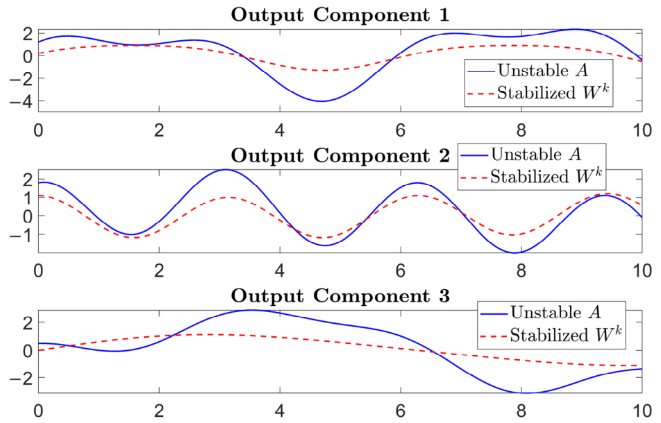
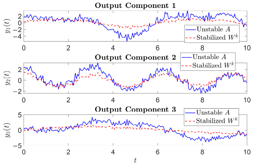
Due to the chosen values of the matrix A, the amplitude of the output varies rapidly over time (Figure 1).

Figure 1 clearly illustrates the limitation of amplitude growth and the smoothing of the signal dynamics when the stabilizing block is applied.

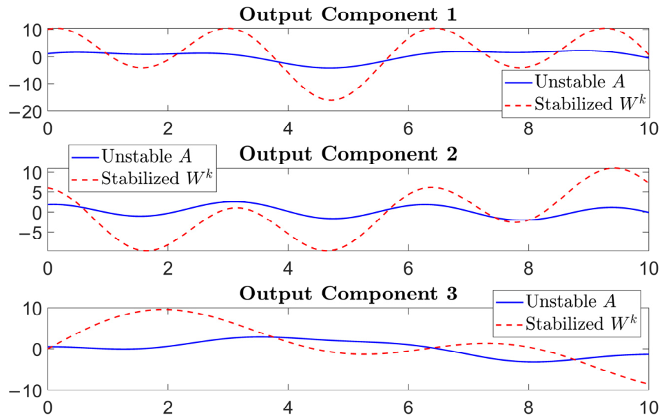
The sensitivity to the parameter $\mu$ is illustrated in Figure 2. For excessively large values (e.g., $\mu =5$), the algebraic correction becomes dominant and leads to undesirable deformation of the output. In this case, the stabilized signal may appear less stable than the unstabilized one. This confirms that the parameters of the stabilizing block must be selected in accordance with the guidelines in Section 3.4.

Table 1. Quantitative results of stabilization under multi-component harmonic input (overall and component-wise metrics).

Component	Output Signal Energy		Standard Deviation		Peak Amplitude		Crest Factor
	${\mathit{E}}_{\mathit{r}\mathit{a}\mathit{w}}$	${\mathit{E}}_{\mathit{s}\mathit{t}\mathit{a}\mathit{b}}$	${\mathsf{\sigma }}_{\mathit{i},\mathit{r}\mathit{a}\mathit{w}}$	${\mathsf{\sigma }}_{\mathit{i},\mathit{s}\mathit{t}\mathit{a}\mathit{b}}$	${\mathbf{A}}_{\mathit{i},\mathit{r}\mathit{a}\mathit{w}}$	${\mathit{A}}_{\mathit{i},\mathit{s}\mathit{t}\mathit{a}\mathit{b}}$	${\mathit{C}\mathit{F}}_{\mathit{i},\mathit{r}\mathit{a}\mathit{w}}$	${\mathit{C}\mathit{F}}_{\mathit{i},\mathit{s}\mathit{t}\mathit{a}\mathit{b}}$
Overall	1801.976	362.647	–	–	–	–	–	–
$y_1\left(t\right)$	–	–	1.8845	0.7212	4.0548	1.2998	2.0995	1.7347
$y_2\left(t\right)$	–	–	1.2730	0.7978	2.5053	1.1988	1.9384	1.5045
$y_3\left(t\right)$	–	–	1.8986	0.7681	3.1455	1.1174	1.6556	1.4228

presents the quantitative results for the unstabilized and stabilized signals. The total energy is computed over the entire signal, while the remaining metrics are reported per component.

The quantitative results indicate a substantial reduction in the total output energy—approximately 80%—demonstrating effective suppression of amplitude growth. The standard deviation is reduced by 37% to 62%, indicating smoother temporal dynamics. The maximum amplitude decreases by up to approximately 68%, while the Crest Factor is reduced by 15–22%, indicating suppression of sharp peaks.

Importantly, stabilization is achieved without significant distortion of the functional structure of the signal. This demonstrates that the algebraic construction $W^k=I+\mu D$ provides control over the signal dynamics without aggressive filtering or loss of structural information.

Overall, the results show that the algebraically stabilizing block acts as an effective mechanism for controlling amplitude dynamics under smooth multi-component input, while preserving the essential structure of the signal.

4.2.2. One-Step INT8-Quantized Experiment

This experiment examines whether the proposed algebraically stabilizing block retains its stabilizing effect under limited numerical precision, specifically in an INT8-quantized arithmetic setting.

In this one-step setting, the stabilizing operator is defined by

$$W=I+\mu D,\mu =1, k=1.$$

(38)

The choice $k=1$ is consistent with the one-step nature of the experiment.

The unstabilized and stabilized operators are applied once to the quantized input. The corresponding output signals are denoted by

$$y_{raw}\left(t\right)=Ax\left(t\right),y_{stab}\left(t\right)=Wx\left(t\right).$$

(39)

where both expressions denote the respective quantized evaluations.

After dequantization, total output signal energy, component-wise standard deviation, maximum amplitude, crest factor, and saturation count are evaluated.

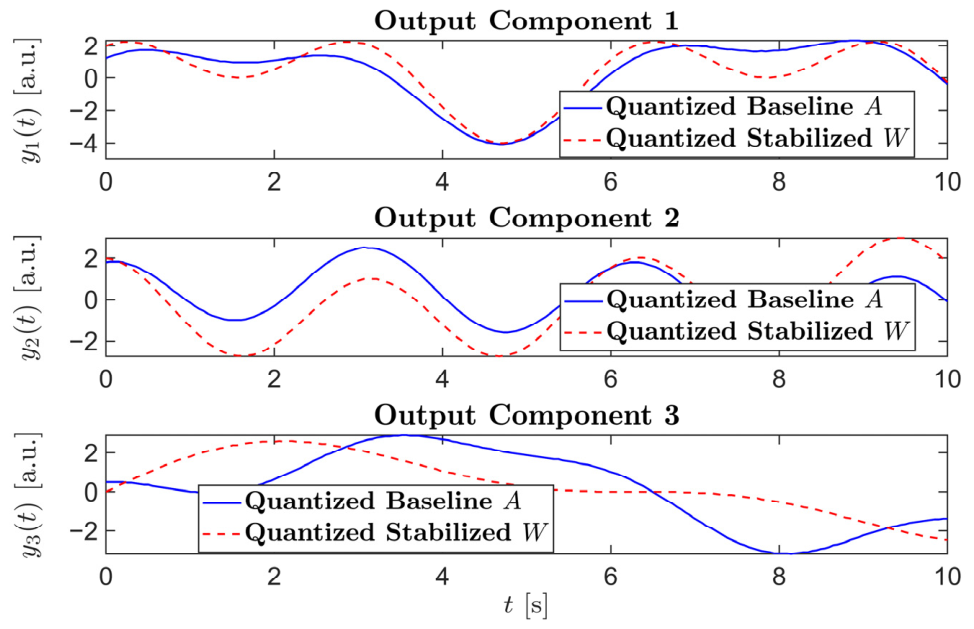
The results show that the algebraically stabilizing block retains part of its observed stabilizing effect under INT8 quantization, although the effect is more moderate than in the floating-point experiment (Figure 3).

In the conducted simulation, the total output signal energy decreases from $E_{raw}=1801.3655$ to $E_{stab}=1647.0338$, which corresponds to an approximate reduction of $8.5\%$. This result indicates that the stabilizing operator reduces the accumulated output energy even under INT8 quantization.

Table 2. Quantitative results of stabilization under multi-component harmonic input in the one-step INT8-quantized experiment (overall and component-wise metrics).

Component	Output Signal Energy		Standard Deviation		Peak Amplitude		Crest Factor		Saturation Count
	${\mathit{E}}_{\mathit{r}\mathit{a}\mathit{w}}$	${\mathit{E}}_{\mathit{s}\mathit{t}\mathit{a}\mathit{b}}$	${\mathsf{\sigma }}_{\mathit{i},\mathit{r}\mathit{a}\mathit{w}}$	${\mathsf{\sigma }}_{\mathit{i},\mathit{s}\mathit{t}\mathit{a}\mathit{b}}$	${\mathbf{A}}_{\mathit{i},\mathit{r}\mathit{a}\mathit{w}}$	${\mathit{A}}_{\mathit{i},\mathit{s}\mathit{t}\mathit{a}\mathit{b}}$	${\mathit{C}\mathit{F}}_{\mathit{i},\mathit{r}\mathit{a}\mathit{w}}$	${\mathit{C}\mathit{F}}_{\mathit{i},\mathit{s}\mathit{t}\mathit{a}\mathit{b}}$	${\mathit{N}}_{\mathit{s}\mathit{a}\mathit{t}}^{\mathit{r}\mathit{a}\mathit{w}}$	${\mathit{N}}_{\mathit{s}\mathit{a}\mathit{t}}^{\mathit{s}\mathit{t}\mathit{a}\mathit{b}}$
Overall	1801.3655	1647.0338	–	–	–	–	–	–	2	2
$y_1\left(t\right)$	–	–	1.882	1.763	4.057	4.000	2.103	2.201	–	–
$y_2\left(t\right)$	–	–	1.268	1.679	2.524	2.992	1.961	1.786	–	–
$y_3\left(t\right)$	–	–	1.903	1.386	3.169	2.614	1.661	1.793	–	–

presents the quantitative results for the unstabilized and stabilized output signals. The total output signal energy and saturation count are computed over the entire signal, whereas the remaining metrics are reported separately for each output component.

The number of saturated values remains identical in both cases: 2. This indicates that, in the one-step INT8 setting, the effect on saturation is limited. The component-wise standard deviation and maximum-amplitude results exhibit mixed behavior. For the first and third output components, the stabilized transformation reduces both standard deviation and maximum amplitude. In contrast, the second component exhibits an increase in these measures. Therefore, a single quantized application is not sufficient for the full structural effect of the algebraically stabilizing block to become uniformly apparent across all output components.

Nevertheless, the experiment has important methodological value. It demonstrates that the proposed block can be implemented and analyzed in an INT8-quantized environment and that its stabilizing effect is not completely lost when moving from floating-point to finite-precision arithmetic. These observations motivate the following repeated-application INT8 experiment, in which the difference between the unstabilized and stabilized transformations becomes more pronounced.

4.2.3. Repeated-Application INT8-Quantized Experiment

This experiment examines whether the proposed algebraically stabilizing block retains its relative advantage under repeated application in an INT8-quantized arithmetic setting. Unlike the one-step experiment, it investigates the accumulation of numerical effects caused by the sequential application of the operators, which is more representative of deep architectures, recurrent structures, and repeated linear modules.

To ensure a consistent comparison between the unstabilized and stabilized transformations, a common operator quantization scale is used for the matrices A and W. The scale is determined by the maximum absolute value of their entries. The input signal and both operators are then quantized to INT8 within the symmetric range [−127,127].

Unlike the one-step INT8 experiment, a fixed state scale is introduced so that, after each iteration, the resulting state is requantized to INT8 using saturation. This simulates repeated operator application under finite-precision conditions. The following parameter values are used:

• state scale: $s_{\mathrm{s}\mathrm{t}\mathrm{a}\mathrm{t}\mathrm{e}}=0.125$;
• operator scale: $s_{\mathrm{o}\mathrm{p}}=0.019685$;
• number of repeated applications: $R=6$.

In both compared schemes, the operators are applied sequentially to the current state. This produces two trajectories:

$$x_{\mathrm{r}\mathrm{a}\mathrm{w}}^{\left(r+1\right)}=A{x}_{\mathrm{r}\mathrm{a}\mathrm{w}}^{\left(r\right)},x_{\mathrm{s}\mathrm{t}\mathrm{a}\mathrm{b}}^{\left(r+1\right)}=W{x}_{\mathrm{s}\mathrm{t}\mathrm{a}\mathrm{b}}^{\left(r\right)},r=0,...,R-1.$$

(40)

The initial states are defined by

$$x_{\mathrm{r}\mathrm{a}\mathrm{w}}^{\left(0\right)}=x_{\mathrm{s}\mathrm{t}\mathrm{a}\mathrm{b}}^{\left(0\right)}=x.$$

(41)

In addition to the INT8 trajectories, floating-point reference trajectories are computed by repeatedly applying the original operators $A$ and $W$, without quantization. This makes it possible to evaluate the accumulated quantization error relative to the corresponding floating-point reference.

At each iteration, the signal energy, saturation count, and quantization error are recorded. After the final iteration, the component-wise standard deviation, maximum amplitude, crest factor, and clipping ratio are also evaluated. The clipping ratio is defined as the ratio between the number of saturated values and the total number of numerical values in the output.

The results show that, under repeated application in the INT8 environment, the difference between the unstabilized and stabilized transformations becomes more pronounced than in the one-step experiment.

After six repeated applications, the total output signal energy is $E_{\mathrm{r}\mathrm{a}\mathrm{w}}=\mathrm{144,839.1563}$ for the unstabilized transformation and $E_{\mathrm{s}\mathrm{t}\mathrm{a}\mathrm{b}}=\mathrm{133,279.3281}$. for the stabilized transformation. This corresponds to an energy reduction of approximately 8% in favor of the stabilized branch.

The final saturation counts are $N_{\mathrm{s}\mathrm{a}\mathrm{t}}^{\mathrm{r}\mathrm{a}\mathrm{w}}=568$ and $N_{\mathrm{s}\mathrm{a}\mathrm{t}}^{\mathrm{s}\mathrm{t}\mathrm{a}\mathrm{b}}=511$, while the corresponding clipping ratios are ${\rho }_{\mathrm{c}\mathrm{l}\mathrm{i}\mathrm{p}}^{\mathrm{r}\mathrm{a}\mathrm{w}}=0.9467$ and ${\rho }_{\mathrm{c}\mathrm{l}\mathrm{i}\mathrm{p}}^{\mathrm{s}\mathrm{t}\mathrm{a}\mathrm{b}}=0.8517$. These results indicate that the stabilized transformation produces fewer saturation events and a lower degree of clipping under repeated application.

The quantization error relative to the floating-point reference is also lower for the stabilized branch. At the end of the experiment, the obtained values are ${\epsilon }_{\mathrm{r}\mathrm{a}\mathrm{w}}=9985.3146$ for the unstabilized transformation and ${\epsilon }_{\mathrm{s}\mathrm{t}\mathrm{a}\mathrm{b}}=7637.7695$ for the stabilized transformation. This corresponds to an approximate reduction of 23.5%, indicating that the stabilizing block accumulates less quantization-induced deformation and exhibits more predictable behavior in the finite-precision setting.

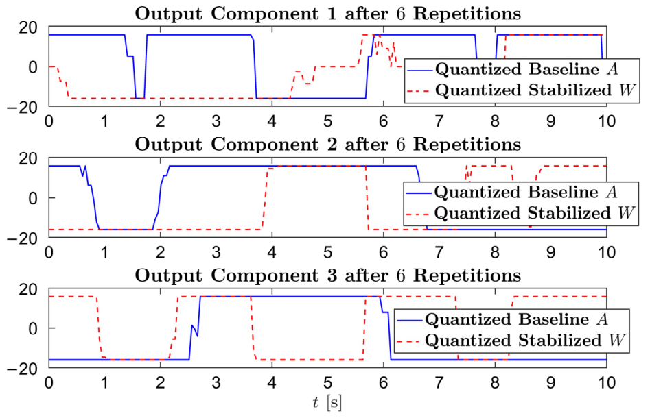
Figure 4 shows that, after six repeated applications, both branches enter a strongly saturated regime, as indicated by the identical maximum amplitude attained by all output components. Nevertheless, the stabilized branch retains lower total energy and exhibits less pronounced accumulation of amplitude deformation.

At the component level, the difference is most evident for the first component, where the standard deviation decreases from 13.504 to 12.728. A smaller but still favorable reduction is observed for the second component. These results indicate that, even under strong quantization-induced saturation, the stabilizing operator limits part of the accumulated dynamic deformation.

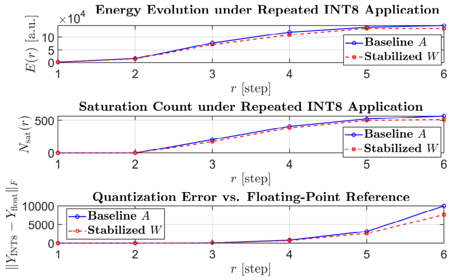
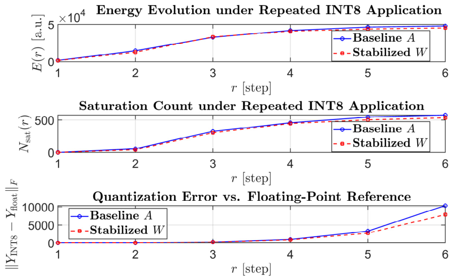
The accumulation of numerical effects resulting from the repeated application of the two operators is illustrated in Figure 5.

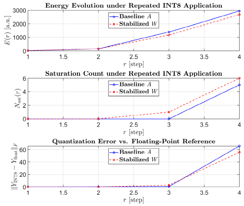
Across all six iterations, the energy of the stabilized branch remains lower than that of the unstabilized transformation, indicating more controlled output growth. The saturation count is also lower for the stabilized operator, reaching 511 compared with 568 for the unstabilized branch. The most pronounced difference is observed for the quantization error relative to the floating-point reference, for which the stabilized branch ends with approximately 23.5% lower accumulated error. This confirms that the proposed block exhibits more predictable behavior under repeated application in a finite-precision environment.

Table 3. Quantitative results, rounded to two decimal places, for stabilization under repeated application in an INT8-quantized environment (overall and component-wise metrics).

Component	Output Signal Energy		Standard Deviation		Peak Amplitude		Crest Factor		Saturation Count		Clipping Ratio		Quantization Error
	${\mathit{E}}_{\mathit{r}\mathit{a}\mathit{w}}$	${\mathit{E}}_{\mathit{s}\mathit{t}\mathit{a}\mathit{b}}$	${\mathsf{\sigma }}_{\mathit{i},\mathit{r}\mathit{a}\mathit{w}}$	${\mathsf{\sigma }}_{\mathit{i},\mathit{s}\mathit{t}\mathit{a}\mathit{b}}$	${\mathbf{A}}_{\mathit{i},\mathit{r}\mathit{a}\mathit{w}}$	${\mathit{A}}_{\mathit{i},\mathit{s}\mathit{t}\mathit{a}\mathit{b}}$	${\mathit{C}\mathit{F}}_{\mathit{i},\mathit{r}\mathit{a}\mathit{w}}$	${\mathit{C}\mathit{F}}_{\mathit{i},\mathit{s}\mathit{t}\mathit{a}\mathit{b}}$	${\mathit{N}}_{\mathit{s}\mathit{a}\mathit{t}}^{\mathit{r}\mathit{a}\mathit{w}}$	${\mathit{N}}_{\mathit{s}\mathit{a}\mathit{t}}^{\mathit{s}\mathit{t}\mathit{a}\mathit{b}}$	${\mathit{\rho }}_{\mathit{c}\mathit{l}\mathit{i}\mathit{p}}^{\mathit{r}\mathit{a}\mathit{w}}$	${\mathit{\rho }}_{\mathit{c}\mathit{l}\mathit{i}\mathit{p}}^{\mathit{s}\mathit{t}\mathit{a}\mathit{b}}$	${\mathit{\epsilon }}_{\mathit{r}\mathit{a}\mathit{w}}$	${\mathit{\epsilon }}_{\mathit{s}\mathit{t}\mathit{a}\mathit{b}}$
Overall	144,839.16	133,279.33	–	–	–	–	–	–	568	511	0.95	0.86	9985.31	7637.77
$y_1\left(t\right)$	–	–	13.50	12.73	15.88	15.88	1.03	1.18	–	–	–	–	–	–
$y_2\left(t\right)$	–	–	15.48	15.22	15.88	15.88	1.02	1.03	–	–	–	–	–	–
$y_3\left(t\right)$	–	–	14.89	15.59	15.88	15.88	1.01	1.01	–	–	–	–	–	–

presents the final numerical results after the sixth iteration. In addition to the standard signal metrics, saturation count, clipping ratio, and quantization error are included because they are particularly relevant for finite-precision analysis.

At the component level, the standard deviation decreases for the first and second output components, whereas a slight increase is observed for the third component. The maximum amplitude reaches the same limiting value in both branches across all components, confirming that the system operates in a strongly saturated regime. Consequently, the crest factor remains close to one and is not the most informative metric in this experiment.

Overall, the repeated-application INT8 experiment shows that the algebraically stabilizing block exhibits a clearer advantage under repeated application than in the one-step setting. The lower output energy, fewer saturation events, lower clipping ratio, and smaller quantization error relative to the floating-point reference indicate more controlled behavior under finite-precision conditions. These findings support the practical relevance of the proposed construction for quantized and hardware-constrained environments.

4.3. Algebraically Stabilizing Block Under Impulsive Inputs

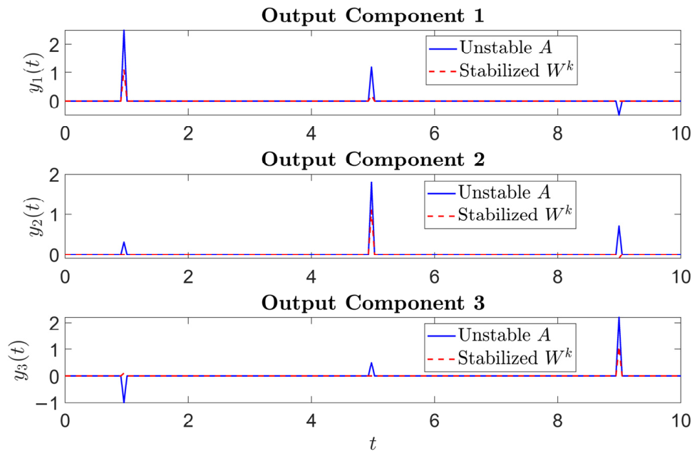
Impulsive signals represent inputs in which only a single component is activated at a given moment, while all other components are zero. Such inputs are characteristic of event-driven systems, spiking neural networks, and reactive architectures. The general form can be written as

$$x\left(t\right)=\delta \left(t-t_0\right)e_i,$$

(42)

where $\delta$ is the Dirac delta function or its discrete counterpart (e.g., the Kronecker delta), $t_0$ denotes the activation time, and $e_i$ is the unit vector with a value of one at the $i$-th position.

Impulsive inputs are particularly sensitive to linear transformations. In a standard neural network, the transformation $Ax\left(t\right)$, when $A$ contains large values, may lead to sharp amplitude peaks or unpredictable responses in the output—especially in networks with integer coefficients, recurrent connections, or layers without normalization.

We consider an input $x\left(t_j\right)\in {\mathbb{R}}^3$ consisting of three impulses at distinct time indices:

$$x\left(t_j\right)=\left[\begin{array}{c}{\delta }_{j,20}\\ {\delta }_{j,100}\\ {\delta }_{j,180}\end{array}\right], j=1,\dots ,200.$$

(43)

where ${\delta }_{j,t}$ denotes the Kronecker delta. Thus, the first, second, and third input components are activated at time indices 20, 100, and 180, respectively.

4.3.1. Floating-Point Experiment

The unstabilized network output is given by

$$y_{raw}\left(t_j\right)=Ax\left(t_j\right).$$

(44)

The stabilizing operator is constructed by

$$W^k=W=I+\mu D,\mu =0.1, k=1.$$

(45)

In the case of impulsive input, we choose $k=1$, since we analyze the instantaneous response of the layer to a localized perturbation rather than the accumulated effect of repeated applications. In this setting, exponentiation is not required to demonstrate the stabilizing effect.

The algebraic stability condition remains satisfied, while the block is applied only once. The stabilized output is

$$y_{stab}\left(t_j\right)=Wx\left(t_j\right).$$

(46)

Figure 6 presents a comparison between $y_{raw}\left(t_j\right)$ and ${ y}_{stab}\left(t_j\right)$ across components. It can be observed that the algebraically stabilizing block limits the spread of the response beyond the location of the impulse and reduces the maximum amplitude without altering the structural form of the signal. This confirms the stabilizing role of the block under highly localized inputs.

Table 4. Quantitative results of stabilization under impulsive input.

Component	Output Signal Energy		Standard Deviation		Peak Amplitude		Threshold Exceedances
	${\mathit{E}}_{\mathit{i},\mathit{r}\mathit{a}\mathit{w}}$	${\mathit{E}}_{\mathit{i},\mathit{s}\mathit{t}\mathit{a}\mathit{b}}$	${\mathsf{\sigma }}_{\mathit{i},\mathit{r}\mathit{a}\mathit{w}}$	${\mathsf{\sigma }}_{\mathit{i},\mathit{s}\mathit{t}\mathit{a}\mathit{b}}$	${\mathbf{A}}_{\mathit{i},\mathit{r}\mathit{a}\mathit{w}}$	${\mathit{A}}_{\mathit{i},\mathit{s}\mathit{t}\mathit{a}\mathit{b}}$	${\mathit{N}}_{0.05,\mathit{r}\mathit{a}\mathit{w}}$	${\mathit{N}}_{0.05,\mathit{s}\mathit{t}\mathit{a}\mathit{b}}$
$y_1\left(t\right)$	7.943	1.250	0.198	0.079	2.5	1.12	3	2
$y_2\left(t\right)$	3.822	1.220	0.137	0.078	1.8	1.14	3	2
$y_3\left(t\right)$	6.094	1.220	0.174	0.078	2.2	1.15	3	2

presents the quantitative results for the unstabilized and stabilized signals.

The peak amplitude in the unstabilized case is significantly higher, while after applying the stabilizing block it is reduced to approximately 1.10–1.15. This indicates that the transformation effectively limits amplitude growth and prevents excessive amplification of the impulse.

The signal energy is also substantially reduced (e.g., from 7.943 to 1.250), demonstrating that the stabilizing block decreases the overall activity induced by the impulse without eliminating the signal itself.

Lower values of the standard deviation indicate a more controlled and less dispersed output dynamics, which is particularly important in settings with limited numerical precision. Furthermore, the reduction in the number of threshold exceedances (from 3 to 2 at threshold $\tau =0.05$) indicates faster decay of the response.

Overall, the results show that applying algebraic stabilization to impulsive inputs:

• limits peak amplitude;
• reduces signal energy;
• accelerates response decay;
• improves numerical stability.

These effects are particularly important for neural networks that must remain robust to sudden inputs (e.g., real-time systems, biomedical diagnostics, anomaly detection), as well as for processing sparse and localized events where controlled and predictable responses are required.

4.3.2. One-Step INT8-Quantized Experiment

This experiment examines the behavior of the proposed algebraically stabilizing block under localized impulsive input in an INT8-quantized arithmetic setting.

The stabilizing operator is defined by

$$W^k=W=I+\mu D,\mu =1, k=1.$$

(47)

The unstabilized and stabilized operators are applied once to the quantized input. The corresponding output signals are given by

$$y_{\mathrm{r}\mathrm{a}\mathrm{w}}\left(t_j\right)=Ax\left(t_j\right),y_{\mathrm{s}\mathrm{t}\mathrm{a}\mathrm{b}}\left(t_j\right)=Wx\left(t_j\right).$$

(48)

where both expressions denote their respective quantized evaluations.

After dequantization, the component-wise output energy, standard deviation, maximum amplitude, threshold-exceedance count, and total saturation count are evaluated.

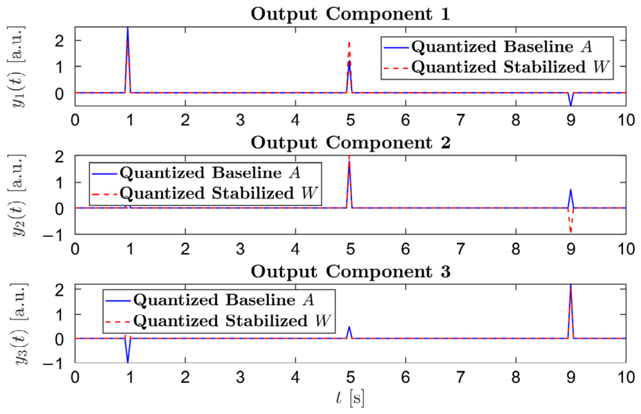
Figure 7 compares the unstabilized and stabilized output signals across the three components. It indicates that the stabilized operator reduces part of the amplitude peaks relative to the unstabilized transformation. Although the effect is not identical across all output components, the stabilized branch produces fewer above-threshold output values.

The results show that the algebraically stabilizing block retains part of its limiting effect under impulsive input in the INT8 environment (

Table 5. Quantitative results of stabilization under impulsive input in the one-step INT8-quantized experiment (overall and component-wise metrics).

Component	Output Signal Energy		Standard Deviation		Peak Amplitude		Threshold Exceedances		Saturation Count
	${\mathit{E}}_{\mathit{i},\mathit{r}\mathit{a}\mathit{w}}$	${\mathit{E}}_{\mathit{i},\mathit{s}\mathit{t}\mathit{a}\mathit{b}}$	${\mathsf{\sigma }}_{\mathit{i},\mathit{r}\mathit{a}\mathit{w}}$	${\mathsf{\sigma }}_{\mathit{i},\mathit{s}\mathit{t}\mathit{a}\mathit{b}}$	${\mathbf{A}}_{\mathit{i},\mathit{r}\mathit{a}\mathit{w}}$	${\mathit{A}}_{\mathit{i},\mathit{s}\mathit{t}\mathit{a}\mathit{b}}$	${\mathit{N}}_{0.05,\mathit{r}\mathit{a}\mathit{w}}$	${\mathit{N}}_{0.05,\mathit{s}\mathit{t}\mathit{a}\mathit{b}}$	${\mathit{N}}_{\mathbf{s}\mathbf{a}\mathbf{t}}^{\mathit{r}\mathit{a}\mathit{w}}$	${\mathit{N}}_{\mathbf{s}\mathbf{a}\mathbf{t}}^{\mathit{s}\mathit{t}\mathit{a}\mathit{b}}$
Overall	–	–	–	–	–	–	–	–	1	0
$y_1\left(t\right)$	7.93	8.06	0.20	0.20	2.5	2.01	3	2	–	–
$y_2\left(t\right)$	3.80	5.04	0.14	0.16	1.79	2.01	3	2	–	–
$y_3\left(t\right)$	6.11	5.04	0.18	0.16	2.20	2.01	3	2	–	–

). The most evident effect is observed in the maximum amplitude, which decreases for the first and third output components. Although the maximum amplitude of the second component increases slightly, it remains within the same range as in the unstabilized case.

The threshold-exceedance count decreases from three to two for all components. This indicates that the stabilized operator reduces the extent to which the localized impulsive events produce above-threshold responses across the output components.

The energy and standard-deviation metrics exhibit mixed component-wise behavior. In particular, the energy increases slightly for the first and second components, whereas it decreases for the third component. The standard deviation remains unchanged for the first component, increases slightly for the second component, and decreases for the third component. Therefore, in the one-step quantized impulsive setting, the primary stabilizing effect is not a uniform reduction of all global metrics, but rather a limitation of extreme local responses and a reduction in the number of above-threshold events.

The reduction of the saturation count from $N_{\mathrm{s}\mathrm{a}\mathrm{t}}^{raw}=1$ to $N_{\mathrm{s}\mathrm{a}\mathrm{t}}^{stab}=0$ is also practically relevant. It indicates that, in this experimental setting, the proposed block eliminates the boundary-valued output detected in the unstabilized branch and may reduce the risk of saturation under localized impulsive perturbations.

Overall, the one-step INT8-quantized experiment under impulsive input shows that the algebraically stabilizing block does not reduce every metric uniformly. However, it reduces the number of above-threshold output values, limits part of the amplitude peaks, and decreases the observed saturation count. These results support the conclusion that the proposed block can contribute to the control of local output responses to sudden inputs under finite-precision arithmetic.

4.3.3. Repeated-Application INT8-Quantized Experiment

This experiment examines the behavior of the proposed algebraically stabilizing block under repeated application in an INT8-quantized setting with localized impulsive inputs. Unlike the one-step impulsive experiment, the present setting investigates the accumulation of numerical effects resulting from the sequential application of the operators. This is particularly relevant to recurrent architectures, repeated linear modules, and systems that process sparse or sudden input events.

The following parameter values are used:

• state quantization scale $s_{state}=0.166667$;
• operator quantization scale $s_{op}=0.019685$;
• total number of repeated operator applications $R=4$.

For notational simplicity, the two trajectories are represented as

$$x_{raw}^{\left(r+1\right)}=A{x}_{raw}^{\left(r\right)},x_{stab}^{\left(r+1\right)}=W{x}_{stab}^{\left(r\right)},\mathrm{r}=0,...,\mathrm{R}-1,$$

(49)

with initial states

$$x_{raw}^{\left(0\right)}=x_{stab}^{\left(0\right)}=x.$$

(50)

At each step, the resulting states are requantized to the INT8 range. Floating-point reference trajectories are also computed by applying the same operators repeatedly without quantization. This makes it possible to evaluate the accumulated quantization error relative to the corresponding floating-point reference state.

At every repeated-application step, the energy of the current state, the saturation count, and the quantization error are recorded. After the final iteration, the component-wise output energy, standard deviation, maximum amplitude, threshold-exceedance count, crest factor, and clipping ratio are additionally evaluated.

After four applications, the total output-signal energy is $E_{raw}=2947.3889$ for the unstabilized transformation and $E_{stab}=2688.1667$ for the algebraically stabilized operator. This corresponds to an approximately 8.8% reduction in total output energy for the stabilized branch (

Table 6. Quantitative results of stabilization under impulsive input in the repeated-application INT8-quantized experiment (overall and component-wise metrics).

Component	Output Signal Energy		Standard Deviation		Peak Amplitude		Crest Factor		Threshold Exceedances		Saturation Count		Clipping Ratio		Quantization Error
	${\mathit{E}}_{\mathit{r}\mathit{a}\mathit{w}}$	${\mathit{E}}_{\mathit{s}\mathit{t}\mathit{a}\mathit{b}}$	${\mathsf{\sigma }}_{\mathit{i},\mathit{r}\mathit{a}\mathit{w}}$	${\mathsf{\sigma }}_{\mathit{i},\mathit{s}\mathit{t}\mathit{a}\mathit{b}}$	${\mathbf{A}}_{\mathit{i},\mathit{r}\mathit{a}\mathit{w}}$	${\mathit{A}}_{\mathit{i},\mathit{s}\mathit{t}\mathit{a}\mathit{b}}$	${\mathit{C}\mathit{F}}_{\mathit{i},\mathit{r}\mathit{a}\mathit{w}}$	${\mathit{C}\mathit{F}}_{\mathit{i},\mathit{s}\mathit{t}\mathit{a}\mathit{b}}$	${\mathit{N}}_{0.05,\mathit{i}}^{\mathit{r}\mathit{a}\mathit{w}}$	${\mathit{N}}_{0.05,\mathit{i}}^{\mathit{s}\mathit{t}\mathit{a}\mathit{b}}$	${\mathit{N}}_{\mathit{s}\mathit{a}\mathit{t}}^{\mathit{r}\mathit{a}\mathit{w}}$	${\mathit{N}}_{\mathit{s}\mathit{a}\mathit{t}}^{\mathit{s}\mathit{t}\mathit{a}\mathit{b}}$	${\mathit{\rho }}_{\mathit{c}\mathit{l}\mathit{i}\mathit{p}}^{\mathit{r}\mathit{a}\mathit{w}}$	${\mathit{\rho }}_{\mathit{c}\mathit{l}\mathit{i}\mathit{p}}^{\mathit{s}\mathit{t}\mathit{a}\mathit{b}}$	${\mathit{\epsilon }}_{\mathit{r}\mathit{a}\mathit{w}}$	${\mathit{\epsilon }}_{\mathit{s}\mathit{t}\mathit{a}\mathit{b}}$
Overall	2947.39	2688.17	–	–	–	–	–	–	–	–	5	6	$0.008$	$0.010$	65.670	55.787
$y_1\left(t\right)$	940.50	896.06	2.167	2.122	21.167	21.167	9.761	10.000	3	2	–	–	–	–	–	–
$y_2\left(t\right)$	905.39	896.06	2.125	2.111	21.167	21.167	9.949	10.000	3	2	–	–	–	–	–	–
$y_3\left(t\right)$	1101.50	896.06	2.352	2.111	21.167	21.167	9.019	10.000	3	2	–	–	–	–	–	–

).

The quantization error relative to the floating-point reference is ${\epsilon }_{raw}=65.6699$ for the unstabilized transformation and ${\epsilon }_{stab}=55.7868$ for the stabilized operator. Thus, the stabilized branch achieves an approximately 15.0% lower deviation from its corresponding floating-point reference trajectory.

At the component level, the output energy decreases for all three components. The stabilized branch also exhibits lower standard deviations for all components. In addition, the threshold-exceedance count decreases from three to two for each output component. These results indicate that, after repeated application, the stabilized transformation produces fewer output entries exceeding the selected threshold.

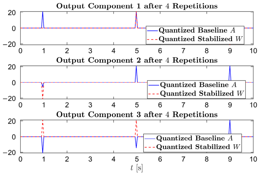
The maximum amplitude reaches the same boundary level in both branches: $A_{i,raw}=A_{i,stab}=21.167$. This shows that both branches reach the same representational boundary under the selected INT8 scaling. Consequently, the maximum amplitude alone does not distinguish the two transformations in this experiment. The crest-factor values are also close in both branches and do not indicate a consistent advantage for the stabilized operator.

The saturation-related metrics do not favor the stabilized branch in this setting: $N_{sat}^{raw}=5,N_{sat}^{stab}=6$ and ${\rho }_{clip}^{raw}=0.0083, {\rho }_{clip}^{stab}=0.0100.$ Thus, the stabilized branch exhibits a slightly higher saturation count and clipping ratio. This result is important because it shows that the proposed construction does not improve every finite-precision metric uniformly under the selected quantization scales and repeated-application setting.

Figure 8 presents the final output signals after four repeated applications of the operators. Both branches reach a similar maximum-amplitude boundary after four applications, in agreement with the numerical results reported above. Nevertheless, the stabilized branch retains lower total energy and lower component-wise standard deviations. The number of threshold exceedances also decreases from three to two for each output component. Therefore, despite reaching the same maximum amplitude, the stabilized operator produces a lower-energy and lower-variance output distribution after repeated application.

Figure 9 shows the accumulation of numerical effects over the repeated-application steps. The most pronounced advantage of the stabilized branch is observed in the quantization error, which decreases from 65.6699 to 55.7868 at the final step. The total output energy is also lower, decreasing from 2947.3889 for the unstabilized transformation to 2688.1667 for the stabilized transformation. In contrast, the saturation count and clipping ratio do not improve for the stabilized branch. Therefore, the principal benefit of the proposed block in this setting lies in lower accumulated energy and closer agreement with the corresponding floating-point dynamics rather than in a reduction of saturation-related effects.

Overall, the repeated-application INT8-quantized experiment under impulsive input shows that the algebraically stabilizing block achieves lower total output energy, lower component-wise standard deviations, fewer threshold-exceedance events, and lower quantization error relative to the floating-point reference. Although the stabilized branch does not improve the saturation count or clipping ratio in this particular setting, the results indicate more controlled numerical behavior in terms of accumulated energy and deviation from the corresponding floating-point trajectory.

4.4. Algebraically Stabilizing Block Under Noisy Inputs

Noise is an inherent component of real-world data. In biomedical measurements, audio, images, and sensor systems, input signals inevitably contain stochastic fluctuations. These random deviations may lead to amplification, instability, and error accumulation in linear or recurrent layers, especially in the absence of normalization or under limited numerical precision.

The proposed algebraically stabilizing block introduces a structurally defined transformation based on the condition $W^k=I+\mu D$. Its purpose in the present setting is to examine whether a structured linear operator can reduce the sensitivity of the output to stochastic input perturbations. In particular, the experiments assess the effect of the stabilizing construction on output energy, component-wise variation, peak amplitudes, and, in the INT8-quantized setting, saturation-related and quantization-related effects.

In the following experiment, a noisy input is simulated by adding a Gaussian component to a smooth signal. The base signal is

$$x_{clean}\left(t\right)=\left[\begin{array}{c}\mathrm{s}\mathrm{i}\mathrm{n}\left(t\right)\\ \mathrm{c}\mathrm{o}\mathrm{s}\left(2\mathrm{t}\right)\\ \mathrm{s}\mathrm{i}\mathrm{n}\left(0.5t\right)\end{array}\right], t\in \left[\mathrm{0,10}\right].$$

(51)

Gaussian noise with zero mean and standard deviation $\sigma =0.2$ is added:

$$x_{noisy}\left(t\right)=x_{clean}\left(t\right)+\eta \left(t\right), \eta \left(t\right)\in \mathcal{N}\left(0, {\sigma }^2\right).$$

(52)

4.4.1. One-Step Floating-Point Experiment

The unstabilized output is

$$y_{raw}\left(t\right)=A{x}_{noisy}\left(t\right).$$

(53)

The stabilizing operator is defined by

$$W^k=W=I+\mu D,\mathsf{\mu }=0.1, k=1.$$

(54)

The stabilized output is

$$y_{stab}\left(t\right)=W^k{x}_{noisy}\left(t\right).$$

(55)

For the analysis, we employ the signal energy and standard deviation metrics, which allow evaluation of noise sensitivity and output variability.

Figure 10 shows that, in the unstabilized case, noise leads to amplification and distortion of the signal, whereas the stabilizing block limits the variation and keeps the amplitude within a controlled range.

Table 7. Quantitative results of stabilization under noisy input (overall and component-wise metrics).

Component	Output Signal Energy		Standard Deviation
	${\mathit{E}}_{\mathit{r}\mathit{a}\mathit{w}}$	${\mathit{E}}_{\mathit{s}\mathit{t}\mathit{a}\mathit{b}}$	${\mathsf{\sigma }}_{\mathit{i},\mathit{r}\mathit{a}\mathit{w}}$	${\mathsf{\sigma }}_{\mathit{i},\mathit{s}\mathit{t}\mathit{a}\mathit{b}}$
Overall	2023.195	401.926	–	–
$y_1\left(t\right)$	–	–	3.947	0.589
$y_2\left(t\right)$	–	–	1.852	0.706
$y_3\left(t\right)$	–	–	4.093	0.654

demonstrates an almost fivefold reduction in total energy (from 2023.2 to 401.9), indicating effective suppression of stochastic amplification.

The standard deviation is significantly reduced across all components (e.g., from approximately 4.0 to 0.6 for $y_1$ and $y_3$), indicating effective suppression of variability around the mean.

Importantly, the reduction in energy does not lead to loss of structural information. The stabilization does not eliminate the useful signal but instead controls the amplitude of the noise component.

Peak-amplitude and threshold-exceedance metrics are not used in this setting, since under stochastic noise, isolated peaks may be random and non-representative. In this context, energy and standard deviation provide more reliable indicators of the global system behavior.

Overall, the results show that under noisy input, the algebraically stabilizing block:

• suppresses stochastic amplification;
• reduces output energy and variance;
• improves numerical stability;
• preserves the structural information of the signal.

This demonstrates that the block can function as an architecture-level mechanism for noise robustness, without requiring external filtering or additional regularization.

4.4.2. One-Step INT8-Quantized Experiment

This experiment examines whether the proposed algebraically stabilizing block retains its limiting effect under noisy input in an INT8-quantized arithmetic setting. In contrast to the deterministic harmonic and localized impulsive inputs considered previously, the present experiment focuses on stochastic input perturbations, which may increase output variability and amplify numerical effects in linear transformations.

The stabilizing operator is defined by

$$W^k=W=I+\mu D,\mu =1, k=1.$$

(56)

The unstabilized and stabilized operators are applied once to the quantized noisy input. The corresponding outputs are given by

$$y_{\mathrm{r}\mathrm{a}\mathrm{w}}\left(t\right)=A{x}_{\mathrm{n}\mathrm{o}\mathrm{i}\mathrm{s}\mathrm{y}}\left(t\right),y_{\mathrm{s}\mathrm{t}\mathrm{a}\mathrm{b}}\left(t\right)=W{x}_{\mathrm{n}\mathrm{o}\mathrm{i}\mathrm{s}\mathrm{y}}\left(t\right),$$

(57)

where both expressions denote their respective quantized evaluations.

After dequantization, the total output-signal energy, component-wise standard deviation, and total saturation count are evaluated (

Table 8. Quantitative results of stabilization under noisy input in the one-step INT8-quantized experiment (overall and component-wise metrics).

Component	Output Signal Energy		Standard Deviation		Saturation Count
	${\mathit{E}}_{\mathit{r}\mathit{a}\mathit{w}}$	${\mathit{E}}_{\mathit{s}\mathit{t}\mathit{a}\mathit{b}}$	${\mathsf{\sigma }}_{\mathit{i},\mathit{r}\mathit{a}\mathit{w}}$	${\mathsf{\sigma }}_{\mathit{i},\mathit{s}\mathit{t}\mathit{a}\mathit{b}}$	${\mathit{N}}_{\mathbf{s}\mathbf{a}\mathbf{t}}^{\mathit{r}\mathit{a}\mathit{w}}$	${\mathit{N}}_{\mathbf{s}\mathbf{a}\mathbf{t}}^{\mathit{s}\mathit{t}\mathit{a}\mathit{b}}$
Overall	1906.745	1721.980	–	–	1	1
$y_1\left(t\right)$	–	–	1.927	1.827	–	–
$y_2\left(t\right)$	–	–	1.314	1.695	–	–
$y_3\left(t\right)$	–	–	1.971	1.426	–	–

).

The total output-signal energy decreases from $E_{raw}=1906.7452$ to $E_{stab}=1721.9799$, which corresponds to an approximately 9.7% reduction. This result indicates that the stabilized transformation reduces the overall magnitude of the output induced by the noisy input under finite-precision arithmetic.

The component-wise standard deviation decreases from 1.927 to 1.827 for the first output component and from 1.971 to 1.426 for the third output component. In contrast, the standard deviation of the second component increases from 1.314 to 1.695.

Thus, the effect of the stabilized operator is not uniform across all output components in the one-step INT8-quantized noisy setting.

The saturation count remains unchanged: $N_{\mathrm{s}\mathrm{a}\mathrm{t}}^{\mathrm{r}\mathrm{a}\mathrm{w}}=1, N_{\mathrm{s}\mathrm{a}\mathrm{t}}^{\mathrm{s}\mathrm{t}\mathrm{a}\mathrm{b}}=1$. Therefore, the stabilized operator does not provide an advantage with respect to the observed saturation count in this particular setting, but it also does not worsen this metric.

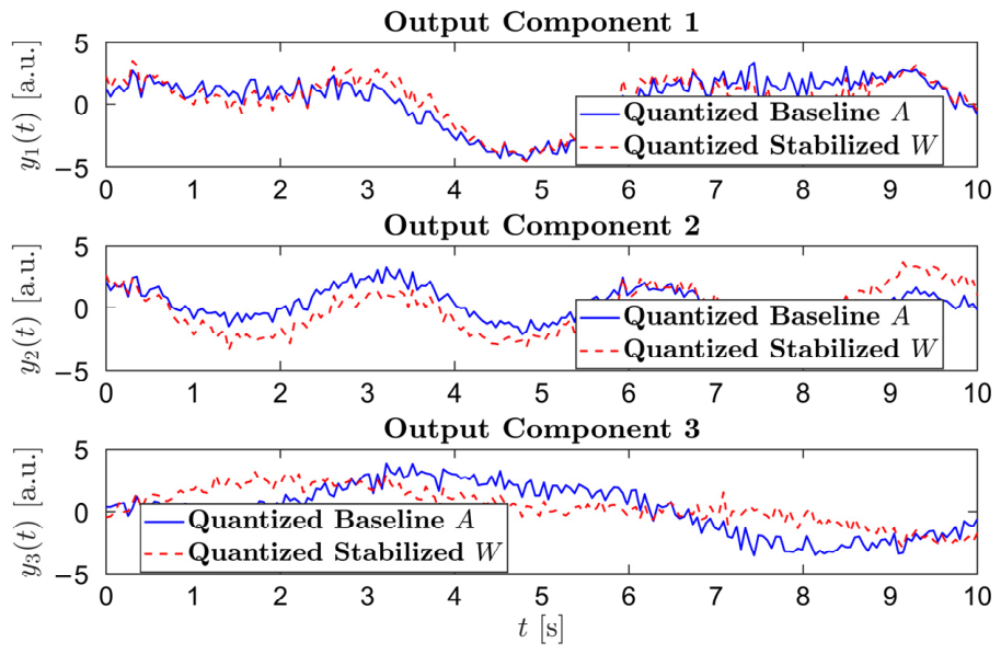
Figure 11 compares the unstabilized and algebraically stabilized outputs across the three components.

Overall, the one-step INT8-quantized experiment under noisy input shows that the algebraically stabilizing block reduces the total output-signal energy and decreases the variation of two of the three output components. Although the component-wise effect is not uniform and no improvement is observed in the saturation count, the results remain consistent with the role of the proposed block as a mechanism for limiting the overall amplification of stochastic input perturbations under finite-precision arithmetic.

4.4.3. Repeated-Application INT8-Quantized Experiment

This experiment examines the behavior of the proposed algebraically stabilizing block under repeated application in an INT8-quantized setting with noisy input. Unlike the one-step noisy-input experiment, the present setting investigates the accumulation of numerical effects resulting from the sequential application of the operators. This is particularly relevant to deep and recurrent architectures, in which stochastic fluctuations may be amplified at successive processing steps.

The same noisy input signal defined in (52), the common unstabilized transformation $A$, and the stabilizing operator $W$ defined in (56) are used.

The following parameter values are used:

• state quantization scale $s_{\mathrm{s}\mathrm{t}\mathrm{a}\mathrm{t}\mathrm{e}}=0.071429$;
• operator quantization scale $s_{\mathrm{o}\mathrm{p}}=0.019685$;
• total number of repeated operator applications $\mathrm{R}=6$.

The two trajectories are represented as

$$x_{raw}^{\left(r+1\right)}=A{x}_{raw}^{\left(r\right)},x_{stab}^{\left(r+1\right)}=W{x}_{stab}^{\left(r\right)},\mathrm{r}=0,...,\mathrm{R}-1,$$

(58)

with initial states

$$x_{raw}^{\left(0\right)}=x_{stab}^{\left(0\right)}=x_{\mathrm{n}\mathrm{o}\mathrm{i}\mathrm{s}\mathrm{y}}.$$

(59)

At each step, the resulting states are requantized to the INT8 range. Floating-point reference trajectories are also computed by repeatedly applying the same operators without quantization. This makes it possible to evaluate the accumulated quantization error relative to the corresponding floating-point reference state.

At every repeated-application step, the energy of the current state, the saturation count, and the quantization error are recorded. After the final iteration, the component-wise standard deviation, maximum amplitude, and clipping ratio are additionally evaluated (

Table 9. Quantitative results of stabilization under noisy input in the repeated-application INT8-quantized experiment.

Component	Output Signal Energy		Standard Deviation		Peak Amplitude		Saturation Count		Clipping Ratio		Quantization Error
	${\mathit{E}}_{\mathit{r}\mathit{a}\mathit{w}}$	${\mathit{E}}_{\mathit{s}\mathit{t}\mathit{a}\mathit{b}}$	${\mathsf{\sigma }}_{\mathit{i},\mathit{r}\mathit{a}\mathit{w}}$	${\mathsf{\sigma }}_{\mathit{i},\mathit{s}\mathit{t}\mathit{a}\mathit{b}}$	${\mathbf{A}}_{\mathit{i},\mathit{r}\mathit{a}\mathit{w}}$	${\mathit{A}}_{\mathit{i},\mathit{s}\mathit{t}\mathit{a}\mathit{b}}$	${\mathit{N}}_{\mathit{s}\mathit{a}\mathit{t}}^{\mathit{r}\mathit{a}\mathit{w}}$	${\mathit{N}}_{\mathit{s}\mathit{a}\mathit{t}}^{\mathit{s}\mathit{t}\mathit{a}\mathit{b}}$	${\mathit{\rho }}_{\mathit{c}\mathit{l}\mathit{i}\mathit{p}}^{\mathit{r}\mathit{a}\mathit{w}}$	${\mathit{\rho }}_{\mathit{c}\mathit{l}\mathit{i}\mathit{p}}^{\mathit{s}\mathit{t}\mathit{a}\mathit{b}}$	${\mathit{\epsilon }}_{\mathit{r}\mathit{a}\mathit{w}}$	${\mathit{\epsilon }}_{\mathit{s}\mathit{t}\mathit{a}\mathit{b}}$
Overall	47,903.27	45,246.02	–	–	–	–	574	534	0.957	0.890	10,348.21	7865.63
$y_1\left(t\right)$	–	–	8.26	8.07	9.07	9.07	–	–	–	–	–	–
$y_2\left(t\right)$	–	–	8.72	8.21	9.07	9.07	–	–	–	–	–	–
$y_3\left(t\right)$	–	–	8.83	8.65	9.07	9.07	–	–	–	–	–	–

).

After $R=6$ applications, the total output-signal energy is $E_{\mathrm{r}\mathrm{a}\mathrm{w}}=\mathrm{47,903}.2704$ for the unstabilized transformation and $E_{\mathrm{s}\mathrm{t}\mathrm{a}\mathrm{b}}=\mathrm{45,246}.0153$ for the algebraically stabilized operator. This corresponds to an approximately 5.5% reduction in total output energy for the stabilized branch.

The quantization error relative to the floating-point reference is ${\epsilon }_{\mathrm{r}\mathrm{a}\mathrm{w}}=\mathrm{10,348.2073}$, ${\epsilon }_{\mathrm{s}\mathrm{t}\mathrm{a}\mathrm{b}}=7865.6319$. Thus, the stabilized branch achieves an approximately 24.0% lower deviation from its corresponding floating-point reference trajectory.

The saturation-related metrics—Saturation Count and Clipping Ratio—also favor the stabilized branch. These results indicate that the stabilized transformation reduces the observed saturation count and the relative proportion of boundary-valued elements under repeated finite-precision processing.

At the component level, the standard deviation decreases for all three output components. The maximum amplitude reaches the same representational boundary in both branches: $A_{i,\mathrm{r}\mathrm{a}\mathrm{w}}=A_{i,\mathrm{s}\mathrm{t}\mathrm{a}\mathrm{b}}=9.0714,\mathrm{i}=1,2,3$. This indicates that both branches reach the same maximum representable level under the selected INT8 state scale. Nevertheless, the remaining metrics show that the stabilized branch retains lower overall energy and lower component-wise standard deviation.

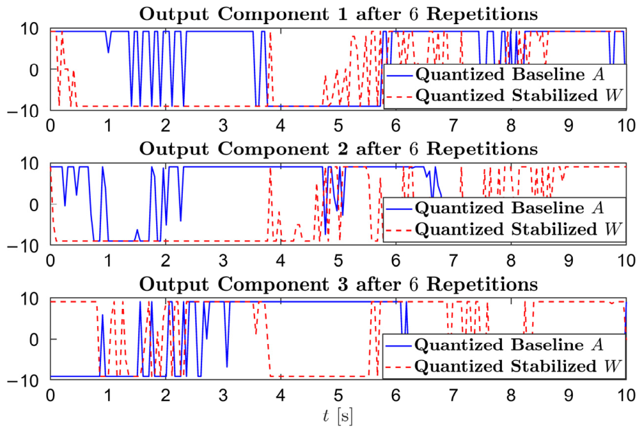
Figure 12 presents the final output signals after six repeated applications of the operators. It shows that both branches reach the same maximum-amplitude boundary after repeated application. However, the stabilized branch exhibits lower overall variation across the output components, consistent with the numerical results reported in Table 9.

Figure 13 shows the accumulation of numerical effects during repeated application. At the final step, the stabilized branch has lower total output energy and lower quantization error than the unstabilized branch. It also exhibits a lower saturation count. Therefore, in this setting, the principal benefit of the proposed block is reflected not only in lower accumulated energy and closer agreement with the floating-point trajectory, but also in reduced saturation-related effects.

Overall, the repeated-application INT8-quantized experiment under noisy input shows that the algebraically stabilizing block achieves lower total output energy, lower component-wise standard deviation, a lower saturation count, a lower clipping ratio, and substantially lower quantization error relative to the floating-point reference. These findings support the conclusion that the proposed operator produces more controlled and predictable numerical behavior under stochastic input perturbations in a finite-precision setting.

4.5. Summary of Experimental Results

The experiments conducted under multi-component harmonic, impulsive, and noisy inputs provide a proof-of-concept evaluation of the proposed algebraically stabilizing block in both floating-point and INT8-quantized settings. The results show that the proposed construction can influence output energy, component-wise variation, peak amplitudes, threshold-exceedance behavior, and finite-precision deviations under different input conditions.

Overall, the results do not indicate a uniform improvement in every metric and in every experimental setting. Nevertheless, the stabilized transformation frequently achieves lower output energy and reduced component-wise variation. In the repeated-application INT8 experiments, it also exhibits lower quantization error relative to the corresponding floating-point reference in all considered input scenarios. The saturation-related metrics depend more strongly on the input type and quantization parameters: they improve in the repeated noisy-input experiment but not in the repeated impulsive-input setting.

The low-dimensional case $n=3$ was deliberately selected to ensure direct visual interpretation of the stabilization effect. The present experiments should therefore be understood as a proof-of-concept demonstration of structurally controlled behavior rather than as evidence of identical quantitative effects in larger neural architectures. For higher-dimensional settings, the sensitivity to $\mu$, $k$, and ${‖D‖}_2$ requires further analysis, while practical implementations may benefit from structured matrices such as sparse, diagonal, banded, or block-based forms.

5. Discussion

The proposed approach is based on a structural algebraic construction in which the behavior of a linear transformation is constrained through a formal condition of the form $W^k=I+\mu D$. Its principal significance in the present work is not that it automatically guarantees classical asymptotic or spectral stability in ${\mathbb{R}}^n$. Rather, it imposes algebraically controlled $k$-step behavior and, in the integer-valued setting, modular predictability. Accordingly, the proposed block should primarily be interpreted as a mechanism for the structural control of repeated linear transformations, rather than as a universal criterion for contractive or Lyapunov-stable dynamics. This distinction is essential. The theoretical results show that, when the condition $W^k=I+\mu D$ is satisfied, the deviation of $W^k$ from the identity operator is algebraically specified by the correction term $\mu D$, while the integer-valued formulation additionally provides modular periodicity. However, this does not automatically imply that every real-valued iterative dynamics induced by W is bounded or that exponential growth is excluded in the classical sense. Therefore, the claims obtained in the present work should be interpreted as claims of algebraic and modular stabilization of a linear block, rather than as a general theorem of spectral stability for arbitrary neural-network dynamics.

From an experimental perspective, the results indicate that this algebraic construction can produce practically observable effects in both real-valued and finite-precision settings. Across harmonic, impulsive, and noisy inputs, the stabilizing block frequently reduces output energy, component-wise standard deviation, and selected amplitude-related measures while preserving the qualitative structure of the transformed signal. The floating-point experiments should be interpreted as illustrative relaxations of the integer-valued theory, designed to demonstrate the mechanism in an interpretable continuous-valued setting. By contrast, the INT8 experiments provide a more direct connection to the original finite-precision motivation. In the repeated-application INT8 experiments, the stabilized branch consistently exhibits lower quantization error relative to the corresponding floating-point reference trajectory. The saturation count and clipping ratio, however, depend more strongly on the input type and quantization parameters: they improve in the repeated noisy-input experiment, whereas no corresponding improvement is observed in the repeated impulsive-input setting. Thus, the experimental findings do not indicate uniform improvement in every metric, but they support the role of the proposed construction as a structured mechanism for reducing selected forms of output amplification and finite-precision deviation.

Additional norm-matched control experiments suggest that the observed effects are not attributable solely to a lower operator magnitude or to closer proximity to the identity transformation. Instead, they indicate that the algebraic structure of the proposed operator may itself contribute to the control of peak responses and output dynamics.

Preliminary proof-of-concept experiments with a trained recurrent neural network further suggest that the proposed block can also be integrated into trainable recurrent architectures. A more systematic evaluation on larger datasets and diverse real-world tasks remains necessary.

The present construction should primarily be regarded as a fixed structural module. Exact maintenance of the constraint $W^k=I+\mu D$ during gradient-based training is straightforward for $k=1$, whereas the general case $k>1$ raises additional parameterization, differentiability, and computational-cost issues. Similarly, for non-square layers of the form $QWP$, the exact algebraic property remains associated with the internal square block $W$, while the behavior of the complete composition also depends on the norms and conditioning of $P$ and $Q$.

The proposed approach is related to quantized neural networks, integer-only inference, norm-based stabilization, and orthogonal or unitary architectures, but it differs in its central objective. Rather than directly minimizing an operator norm or enforcing orthogonality, it introduces an explicit algebraic constraint that specifies predictable $k$-step behavior of an internal linear block. Thus, the main contribution is a structurally defined mechanism for algebraic and modular control, which can produce favorable numerical effects in finite-precision settings. Future work should address trainable parameterizations, stronger real-valued guarantees under additional assumptions, and larger-scale integration into quantized and recurrent architectures.

6. Conclusions

This work proposed a construction of algebraically stabilizing blocks for quantized and finite-precision neural networks, based on a condition of the form ${ W}^k=I+\mu D$.

The analysis shows that this condition specifies algebraically controlled $k$-step behavior of the linear block and provides modular periodicity in the integer-valued setting. The construction is also invariant under the considered conjugation transformations, which supports its transfer across equivalent linear representations.

A principal contribution of the work is the formulation of the stabilizing mechanism as a local architectural module that can be embedded into more general neural-network structures, including quantized and hardware-constrained environments. The experimental results under harmonic, impulsive, and noisy inputs, including INT8-quantized settings, show that the proposed block can, in several cases, reduce output energy, component-wise variation, selected amplitude-related measures, and finite-precision deviation relative to floating-point reference trajectories. The norm-matched control experiments further suggest that the observed effects are not attributable solely to a lower operator magnitude, but may also reflect structural properties of the algebraically constructed operator.

At the same time, it is important to emphasize that the obtained results concern algebraic and modular stabilization of the linear block rather than a general guarantee of classical spectral or asymptotic stability in real-valued space. The proposed approach does not replace existing norm-based or orthogonality-based stabilization techniques. Instead, it provides a complementary structural mechanism that is particularly relevant to quantized and finite-precision settings.

Natural directions for future work include the derivation of stronger real-valued results under additional spectral assumptions, the development of trainable parameterizations of $D$, systematic scaling to higher-dimensional settings, and the integration of the proposed block into more complex quantized and recurrent architectures. Overall, the results indicate that algebraically specified linear blocks can serve as formally defined structural modules for controlling repeated linear transformations in neural networks, particularly under limited numerical precision.

References

1. Purnomo, A.; Tjandrasa, H. Improved Deep Learning Architecture with Batch Normalization for EEG Signal Processing. J. Ilm. Teknol. Inf. 2021, 19, 19–27. [Google Scholar] [CrossRef]
2. Ziaee, A.; Çano, E. Batch Layer Normalization: A New Normalization Layer for CNNs and RNNs. In Proceedings of the 6th International Conference on Advances in Artificial Intelligence, Birmingham, UK, 21–23 October 2022; pp. 40–49. [Google Scholar] [CrossRef]
3. Peng, H.; Yu, Y.; Yu, S. Re-thinking the Effectiveness of Batch Normalization and Beyond. IEEE Trans. Pattern Anal. Mach. Intell. 2023, 46, 465–478. [Google Scholar] [CrossRef] [PubMed]
4. Ruhland, J.B.; Masoudian, I.; Heider, D. Enhancing Deep Neural Network Training through Learnable Adaptive Normalization. Knowl.-Based Syst. 2025, 326, 113968. [Google Scholar] [CrossRef]
5. Gogianu, F.; Berariu, T.; Rosca, M.C.; Clopath, C.; Busoniu, L.; Pascanu, R. Spectral Normalisation for Deep Reinforcement Learning: An Optimisation Perspective. In Proceedings of the International Conference on Machine Learning (ICML), Virtual, 18–24 July 2021; pp. 3734–3744. [Google Scholar]
6. Keriven, N. Not Too Little, Not Too Much: A Theoretical Analysis of Graph (Over)Smoothing. Adv. Neural Inf. Process. Syst. 2022, 35, 2268–2281. [Google Scholar] [CrossRef]
7. Shi, Z.; Mettes, P.; Maji, S.; Snoek, C.G.M. On Measuring and Controlling the Spectral Bias of the Deep Image Prior. Int. J. Comput. Vis. 2022, 130, 885–908. [Google Scholar] [CrossRef]
8. Zhai, S.; Likhomanenko, T.; Littwin, E.; Busbridge, D.; Ramapuram, J.; Zhang, Y.; Susskind, J.M. Stabilizing Transformer Training by Preventing Attention Entropy Collapse. In Proceedings of the International Conference on Machine Learning (ICML), Honolulu, HI, USA, 23–29 July 2023; pp. 40770–40803. [Google Scholar]
9. Wang, R.; An, S.; Liu, W.; Li, L. Invertible Residual Blocks in Deep Learning Networks. IEEE Trans. Neural Netw. Learn. Syst. 2023, 35, 10167–10173. [Google Scholar] [CrossRef] [PubMed]
10. Selvaraju, K.; Rajamani, S. New Approach to Underwater Image Enhancement Using Modified Residual Blocks in Generator Architecture for Improved Cycle Generative Adversarial Networks. C. R. Acad. Bulg. Sci. 2024, 77, 73–81. [Google Scholar] [CrossRef]
11. Eskandari, H.; Imani, M.; Moghaddam, M.P. A Deep Residual Network Integrating Entropy-Based Wavelet Packet Ensemble Model for Short-Term Electrical Load Forecasting. Energy 2025, 314, 134168. [Google Scholar] [CrossRef]
12. Yotov, K.; Hadzhikolev, E.; Hadzhikoleva, S. Algebraic Stabilization of Linear Transformations in Artificial Neural Networks. Mathematics 2026, 14, 623. [Google Scholar] [CrossRef]
13. Yotov, K.; Hadzhikolev, E. Conjugational Stability and Symmetry-Invariant Transformations in Artificial Neural Networks. Comput. Sci. Interdiscip. Res. J. 2026, 3, 1–18. [Google Scholar] [CrossRef]
14. Huang, L.; Yang, D.; Lang, B.; Deng, J. Decorrelated Batch Normalization. In Proceedings of the IEEE Conference on Computer Vision and Pattern Recognition (CVPR), Salt Lake City, UT, USA, 18–23 June 2018; pp. 791–800. [Google Scholar] [CrossRef]
15. Mobasseri, B.G.; Lulu, A. Radiometric Identification of Signals by Matched Whitening Transform. Sensors 2021, 21, 8398. [Google Scholar] [CrossRef] [PubMed]
16. Zhang, C.; Zheng, Y.; Guo, B.; Li, C.; Liao, N. SCN: A Novel Shape Classification Algorithm Based on Convolutional Neural Network. Symmetry 2021, 13, 499. [Google Scholar] [CrossRef]
17. Zhang, S.; Nezhadarya, E.; Fashandi, H.; Liu, J.; Graham, D.; Shah, M. Stochastic Whitening Batch Normalization. In Proceedings of the 2021 IEEE/CVF Conference on Computer Vision and Pattern Recognition (CVPR), Nashville, TN, USA, 20–25 June 2021; pp. 10978–10987. [Google Scholar] [CrossRef]
18. Xu, J.; Kim, H.; Rainforth, T.; Teh, Y.W. Group Equivariant Subsampling. Adv. Neural Inf. Process. Syst. 2021, 34, 5934–5946. [Google Scholar] [CrossRef]
19. Favoni, M.; Ipp, A.; Müller, D.I.; Schuh, D. Lattice Gauge Equivariant Convolutional Neural Networks. Phys. Rev. Lett. 2022, 128, 032003. [Google Scholar] [CrossRef] [PubMed]
20. Mirkes, E.M.; Bac, J.; Fouché, A.; Stasenko, S.V.; Zinovyev, A.; Gorban, A.N. Domain Adaptation Principal Component Analysis: Base Linear Method for Learning with Out-of-Distribution Data. Entropy 2022, 25, 33. [Google Scholar] [CrossRef] [PubMed]
21. Simons, T.; Lee, D.-J. A Review of Binarized Neural Networks. Electronics 2019, 8, 661. [Google Scholar] [CrossRef]
22. Jacob, B.; Kligys, S.; Chen, B.; Zhu, M.; Tang, M.; Howard, A.; Adam, H.; Kalenichenko, D. Quantization and training of neural networks for efficient integer-arithmetic-only inference. In Proceedings of the IEEE Conference on Computer Vision and Pattern Recognition, Salt Lake City, UT, USA, 18–22 June 2018; pp. 2704–2713. [Google Scholar] [CrossRef]
23. Novac, P.-E.; Boukli Hacene, G.; Pegatoquet, A.; Miramond, B.; Gripon, V. Quantization and Deployment of Deep Neural Networks on Microcontrollers. Sensors 2021, 21, 2984. [Google Scholar] [CrossRef] [PubMed]
24. Wei, L.; Ma, Z.; Yang, C.; Yao, Q. Advances in the Neural Network Quantization: A Comprehensive Review. Appl. Sci. 2024, 14, 7445. [Google Scholar] [CrossRef]
25. Combettes, P.L.; Pesquet, J.C. Lipschitz certificates for layered network structures driven by averaged activation operators. SIAM J. Math. Data Sci. 2020, 2, 529–557. [Google Scholar] [CrossRef]
26. Helfrich, K.; Willmott, D.; Ye, Q. Orthogonal recurrent neural networks with scaled Cayley transform. In Proceedings of the 35th International Conference on Machine Learning, Stockholm, Sweden, 10–15 July 2018; pp. 1969–1978. Available online: https://proceedings.mlr.press/v80/helfrich18a.html (accessed on 29 June 2026).
27. Lalapura, V.S.; Bhimavarapu, V.R.; Amudha, J.; Satheesh, H.S. A Systematic Evaluation of Recurrent Neural Network Models for Edge Intelligence and Human Activity Recognition Applications. Algorithms 2024, 17, 104. [Google Scholar] [CrossRef]
Figure 1. Comparison between the unstabilized and algebraically stabilized linear transformations under multi-component harmonic input in floating-point arithmetic. The three output components (Output Components 1–3) are shown. (MATLAB R2018a).
Axioms 15 00533 g001
Figure 2. Effect of a large correction parameter μ = 5 on stabilization: comparison of output signals for unstabilized and stabilized transformations under multi-component harmonic input in floating-point arithmetic. The three output components are shown. (MATLAB R2018a).
Axioms 15 00533 g002
Figure 3. Comparison between unstabilized and algebraically stabilized linear transformations under multi-component harmonic input in an INT8-quantized arithmetic setting. The three output components (Output Components 1–3) are shown. (MATLAB R2018a).
Axioms 15 00533 g003
Figure 4. Comparison between unstabilized and algebraically stabilized transformations after repeated application in an INT8-quantized environment. The three output components are shown after the final iteration. (MATLAB R2018a).
Axioms 15 00533 g004
Figure 5. Evolution of output energy, saturation count, and quantization error during repeated application of the unstabilized and algebraically stabilized transformations in an INT8 environment. (MATLAB R2018a).
Axioms 15 00533 g005
Figure 6. Response of a linear transformation under impulsive input: comparison between unstabilized and stabilized transformations. The three output components (Output Components 1–3) are shown. (MATLAB R2018a).
Axioms 15 00533 g006
Figure 7. Response of a linear transformation under impulsive input in an INT8-quantized arithmetic setting: comparison between unstabilized and algebraically stabilized transformations. The three output components (Output Components 1–3) are shown. (MATLAB R2018a).
Axioms 15 00533 g007
Figure 8. Comparison between the unstabilized and algebraically stabilized transformations after repeated application under impulsive input in an INT8-quantized environment. The three output components after the final iteration are shown. (MATLAB R2018a).
Axioms 15 00533 g008
Figure 9. Evolution of output-signal energy, saturation count, and quantization error under repeated application of the unstabilized and algebraically stabilized transformations with impulsive input in an INT8-quantized environment. (MATLAB R2018a).
Axioms 15 00533 g009
Figure 10. Response of a linear transformation under noisy input in floating-point arithmetic: comparison between unstabilized and algebraically stabilized transformation ( μ = 0.1 ,   k = 1 ). The three output components (Output Components 1–3) are shown. (MATLAB R2018a).
Axioms 15 00533 g010
Figure 11. Response of a linear transformation under noisy input in an INT8-quantized arithmetic setting: comparison between unstabilized and algebraically stabilized transformations. The three output components (Output Components 1–3) are shown. (MATLAB R2018a).
Axioms 15 00533 g011
Figure 12. Comparison between the unstabilized and algebraically stabilized transformations after repeated application under noisy input in an INT8-quantized environment. The three output components after the final iteration are shown. (MATLAB R2018a).
Axioms 15 00533 g012
Figure 13. Evolution of output-signal energy, saturation count, and quantization error under repeated application of the unstabilized and algebraically stabilized transformations with noisy input in an INT8-quantized environment. (MATLAB R2018a).
Axioms 15 00533 g013