


Abstract
This work introduces Fuzzy Implication Modeling Theory, a connective-centered framework
that supplies an intermediate structural layer between the class and family levels in
the subset of fuzzy implications generated by compositions of the three basic fuzzy
connectives. The theory distinguishes Fuzzy Implication Models from Fuzzy Implication
Model Instances and formalizes their relationship through three propositions addressing
generation, traceability and non-uniqueness. Two model-level quantitative descriptors—a
Behavior Index and an Intra-Model Variability Index—are proposed to enable comparative
analysis across models, and a new Fuzzy Implication Model is introduced and proven
to satisfy the defining conditions of a fuzzy implication. A MATLAB-based companion
tool with a dedicated model-design module operationalizes the theory. Taken together,
the framework provides a structured lens for organizing, analyzing and selecting fuzzy
implication operators, and opens paths for both further theoretical development and
applied studies.
Keywords:
fuzzy logic; fuzzy implications; fuzzy implication model; computational mathematics; MATLAB; behavioral quantification MSC:
03B52; 03E72; 68T37
1. Introduction
Over the last few years, the world’s news headlines have been dominated by rapid advancements in the space of artificial intelligence. As a result, during such an explosive growth period, it may have been easy to overlook the theoretical work that renders these new applications possible.
One of the fields that remains under-credited for its contributions to artificial intelligence and society in general is fuzzy logic, which combines a particularly active presence in theoretical research with a wide range of useful applications in industry [1], agriculture [2], and even meteorology [3].
The present article builds upon a previous study by the authors [4], extending it from a single new implication model into a general theoretical framework, with the aim of modeling the subset of implications outlined in that study and integrating this new paradigm into the established understanding of the field. Before presenting the framework, the current state of the field is briefly reviewed, in order to make explicit the gap that the framework is designed to fill.
The first step in the process of identifying how implications are organized is mentioning the term fuzzy implication families. Among the principal families documented in the literature are -implications [5], R-implications [5], -implications [6], D-implications [6], and Yager’s f and g-implications [7]. Building upon this framework, fuzzy implication classes can be introduced as broader classifications that may encompass multiple families. Depending on the strategy used in the definition of a given implication family, it can be organized into classes representing families generated from unary functions [7], families generated from other fuzzy implication functions [8], families generated according to their final expression [9,10], or families generated from other fuzzy operators [11,12,13,14]. A finer distinction matters here: special importance should be placed on the composition-based class. The authors hold that the transition from the class level classification straight to the individual families is too general and lacks intermediate structuring. This assessment is supported by three key observations: First, the role of the three basic fuzzy operators—negation, conjunction and disjunction—whose importance in logic far outweighs all others. Second, the existence of underlying connections between the different logical constructs [4] that have not been explicitly studied yet. Third, the simplicity and usefulness displayed by relevant implications, making the creation of a framework centered around them a valuable addition to the field given the advantages it will offer in their study. These observations led to the introduction of a new classification, a “sub-class” that fills the described literature gap and is composed only of implication families arising from combinations of the three basic logical connectives.
Within this sub-class, Fuzzy Implication Modeling is proposed as an efficient and effective way to study its elements. The concept of Fuzzy Implication Models, or F.I.M.s, denotes the subset of implication families that fall under the parameters defined by the new sub-class. The deliberate name change from “family” to “model” reflects the authors’ aim of a differentiated and independent theoretical framework whose scope is clearly defined in relation to the rest of the field, and whose main focus lies in studying the underlying connections among the different logical constructs and how they can be utilized for further research purposes.
Guided by these considerations, the present article revisits and sharpens the ideas introduced in [4] with improved definitions, introduces new constructs that extend the theoretical front around fuzzy implications, exercises them in a limited case study, and packages the whole framework into a companion computer algorithm that elevates its applicability for researchers across domains.
The contribution of this work is fourfold. First, it establishes the notions of a Fuzzy Implication Model and Fuzzy Implication Model Instance, providing a structural layer that is absent from existing class-level and family-level treatments of fuzzy implications. Second, it formulates three propositions characterizing the generative, traceability and non-uniqueness relations between models and instances—results which, by construction, cannot be expressed within a purely class-level or family-level formalism since they refer to the intermediate layer introduced here. Third, it introduces two model-level quantitative descriptors, a Behavior Index and an Intra-Model Variability Index, which make it possible to compare models on a common numerical scale and to quantify the diversity of implications that a single model can generate. Fourth, it proves that a new compositional instance, denoted , is a valid fuzzy implication, and packages the whole framework into a reproducible MATLAB R2025b tool. Taken together, these contributions provide both the vocabulary and the measuring instruments needed to analyse the subset of compositionally-generated fuzzy implications in a systematic way.
2. Preliminaries
The Preliminaries section contains detailed presentations of elemental concepts and ideas used throughout the paper that from this point onward will be considered known by the authors. The motivation behind the inclusion of such a segment is not only to clear up any misunderstandings or inconsistencies but also to render readers of other research backgrounds capable of understanding the paper. Consequently, the authors chose to incorporate the definitions of the following key principles:
- Fuzzy implications
- Triangular norms
- Triangular conorms
- Fuzzy negations
- Mean
- Standard deviation
2.1. Fuzzy Implications
The definition of fuzzy implications presented below is available in the following studies; see, e.g., [15,16,17].
Definition 1.
A binary operator is said to be an implication function, or an implication, if, for all , it satisfies the following:
- (I1):
- is decreasing;
- (I2):
- is increasing;
- (I3):
- boundary condition;
- (I4):
- boundary condition;
- (I5):
- boundary condition.
A function is called a fuzzy implication only if it satisfies –.
The set of all these fuzzy implications will be denoted by .
2.2. Fuzzy Negations
The following definition of fuzzy negations can be found in, e.g., ([15], pp. 13–14) and [18,19,20,21,22].
Definition 2.
A function is called a Fuzzy negation if
- (N1)
- (N2)
- N is decreasing.A fuzzy negation N is called strict if, in addition to the former properties, the following apply:
- (N3)
- N is strictly decreasing;
- (N4)
- N is continuous.A fuzzy negation N is called strong if the following property is satisfied:
- (N5)
2.3. Triangular Norms (Conjunctions)
The definition of triangular norms adopted in this work is consistent with the formulations provided in, e.g., ([23], pp. 4–10), ([15], pp. 41–42), ([21], pp. 116–117), [16].
Definition 3.
A function is called a triangular norm, or a t-norm, if it satisfies, for all , the following conditions:
- (T1)
- (T2)
- (T3)
- (T4)
2.4. Triangular Conorms (Disjunctions)
Triangular conorms are defined in accordance with, e.g., ([23], p. 11), ([15], pp. 45–46), [16].
Definition 4.
A function is called a triangular conorm (or t-conorm) if it satisfies, for all , the following conditions:
- (S1):
- (S2):
- (S3):
- (S4):
2.5. Mean
The concept of the mean is included here due to its involvement in the development of the Fuzzy Implication Model Behavior Index, which will be expanded upon in the main section of the paper. The following definitions are consistent with the formulations provided in, e.g., ([24], pp. 212–213).
Definition 5.
Let be the values of a finite population of size N. The population mean is defined as
Let be a sample of n observations drawn from the population. The sample mean is defined as
2.6. Standard Deviation
Similarly, the standard deviation is included due to its role in the Fuzzy Implication Model Intra-Model Variability Index. The following definitions are consistent with the formulations provided in, e.g., ([24], pp. 212–213).
Definition 6.
The standard deviation measures the dispersion of a set of values around their mean. Let be the values of a finite population of size N with population mean μ. The population standard deviation is defined as
Let be a sample of n observations with sample mean . The sample standard deviation is defined as
where the denominator (Bessel’s correction) yields an unbiased estimator of the population variance.
3. Materials and Methods
3.1. Foundational Concepts
The implementation of the proposed framework requires the adoption of multiple new concepts. Before proceeding to their presentation, it is necessary to first clarify the Fuzzy Implication Model (F.I.M.), which arguably serves as the most pivotal mechanism in Fuzzy Implication Modeling theory. Introduced for the first time in [4], the following definition has been composed for the F.I.M.:
Definition 7.
A function is said to be a Fuzzy Implication Model (F.I.M.) if it satisfies the following:
- (IM1):
- is any high-order composition of the functions , and which symbolize any fuzzy negation, disjunction and conjunction, respectively. The participation of all three fuzzy connectives in any given model composition is not mandatory.
- (IM2):
- is a fuzzy implication.
After defining the Fuzzy Implication Model, the next logical step is proceeding to the introduction of new concepts. To be more specific, the first one is the Fuzzy Implication Model Instance (F.I.M.I. or simply Instance), which acts as a complement to F.I.M. This novel idea is referring to the standalone implications that are generated from a model’s general formula when the fuzzy connective placeholders in it are replaced with specific functions (forming a usable implication). The goal behind the creation of this term is fulfilling the need to refer to individual implications produced from F.I.M.s without generating confusion. The definition of the Fuzzy Implication Model Instance is the following:
Definition 8.
A function is said to be a Fuzzy Implication Model Instance (F.I.M.I.) if it satisfies the following:
- (Im1):
- is a composition comprised of any combination of the three basic fuzzy logical connectives (negation, conjunction and disjunction). The participation of all three fuzzy connectives in any given instance composition is not mandatory.
- (Im2):
- does not include any high-order elements in its composition like or .
- (Im3):
- is a fuzzy implication.
Definition Analysis: The reason behind the inclusion of is so that the term does not extend out of the theory’s scope and describes only the intended subset of implications. Furthermore, the rejection of high-order elements in is aligned with the instance’s characteristic of referring to individual implications and not implication families (models).
It is evident from the definitions of and that the two constructs are closely related to each other, rendering the examination of their interactions a matter of scientific interest. As a consequence, and after conducting said analysis, the authors culminated in the declaration of three propositions that formalize how the two discussed concepts interconnect. However, in order to properly present the given propositions, the utilization of a Fuzzy Implication Model was deemed necessary. The model created for this role can be seen in Theorem 1:
Theorem 1.
Let S, T and N be functions such that:
- , is a fuzzy negation
- , is a triangular norm (t-norm)
- , is a triangular conorm (t-conorm)
Then, there is a fuzzy implication , with the following formula:
Proof.
Let be the function defined by (5). It is shown that satisfies conditions – of Definition 1.
- (I1)
- Monotonicity in the first argument. Let be such that . Since N is a fuzzy negation, it is decreasing, and thus . With the value being fixed and S increasing in each argument, it follows thatBy another application of the monotonicity of S to the outer operator , it is obtained thatHence, is decreasing and is satisfied.
- (I2)
- Monotonicity in the second argument. Let be such that . Since T is increasing in each argument, it is obtained thatAs S is increasing in each argument and is fixed, the inequalityis satisfied. Using again the monotonicity of S and the fact that , it is concluded thatTherefore, is increasing and is satisfied.
- (I3)
- Since N is a fuzzy negation, it follows from that , and thusSince T is a t-norm, it follows from that (by substituting in ). Moreover, since , monotonicity yieldsBecause , it also holds that , hence . Therefore,Since S is a t-conorm, it follows from that (by substituting in ). Consequently,Finally, by commutativity , , and by , . Thus, , and is satisfied.
- (I4)
- Since N is a fuzzy negation, it follows from that , and thusSince T is a t-norm, it follows from that (by substituting in ). Hence,By commutativity and the neutral element property , . Therefore,Since S is a t-conorm, by it holds that . Moreover, since , monotonicity (applied to the second argument with fixed) yieldsThus , and hence . Consequently, , and is satisfied.
- (I5)
- Since N is a fuzzy negation, it follows from that , and thusAs shown in (I3), . Therefore,By , (by substituting in ), henceApplying again with , it is obtained that . Therefore, , and is satisfied.
Since conditions – are satisfied, it is concluded that is a fuzzy implication. □
At this point it is deemed appropriate to move on to the presentation of the above-mentioned propositions. The following propositions are established through constructive demonstration rather than formal proof, as their validity is grounded in the definitional structure of the framework and illustrated through concrete examples.
Proposition 1
(Generation Property). Assume that N is any fuzzy negation and that S, T are any t-conorm/t-norm pair on . Let be a Fuzzy Implication Model in the sense of Definition 7. Every Fuzzy Implication Model can produce an infinite number of Fuzzy Implication Model Instances.
Justification. The validity of this proposition is rooted in the possibility of utilizing parametric connectives in model compositions. In essence, an endless number of implications can be extracted through a single model, since it can be rendered infinitely customizable through connective parameter(s). As an example, the Fuzzy Implication Model of Theorem 1 has been used in the formulation of a parametric instance practically displaying Proposition 1.
To be more specific, starting with the model’s general formula:
subsequently, the following logical connectives are replaced in the appropriate placeholders:
- , Gödel t-conorm
- , Gödel t-norm
- , Sugeno negation
Consequently, the ensuing instance arises:
As it can easily be understood, given the infinite values that the parameter can take, the above instance formula can be customized into limitless variations (instances).
Proposition 2
(Traceability Property). Assume that N is any fuzzy negation and that S, T are any t-conorm/t-norm pair on . Let be a Fuzzy Implication Model in the sense of Definition 7. Every Fuzzy Implication Model Instance is generated by at least one Fuzzy Implication Model in the sense of Definition 7.
Justification. The driving force behind the incorporation of Proposition 2 into the proposed framework is the resolution of one of its main theoretical gaps. To elaborate, even though it has been well-established by this point that instances are a product of Fuzzy Implication Models, there is no reference to the rules that govern the inverse relationships that develop between them. The introduction of the proposition in question aims to settle this vagueness by asserting that all instances (implications that fit into the scope of the theory) can be traced back to a Fuzzy Implication Model. While this property follows naturally from the definitional relationship between F.I.M. and F.I.M.I., its explicit statement is warranted to complete the formal characterization of the bidirectional linkage between models and instances (see in Definition 8).
Proposition 3
(Non-uniqueness Property). Assume that N is any fuzzy negation and that S, T are any t-conorm/t-norm pair on . Let be a Fuzzy Implication Model in the sense of Definition 7. There exist Fuzzy Implication Model Instances that are generated by more than one distinct Fuzzy Implication Model.
Justification. The current proposition originates from an experimental observation made by the authors, where instances generated from different models seemed to converge into shared formulas. The importance of the described phenomenon is significantly elevated when combined with insight gained from the previous two propositions since it rules out the possibility of establishing a one-to-one model-instance relationship.
The following example has been set up in order to practically display Proposition 3. To elaborate, it will demonstrate how two fuzzy implication instances originating from different Fuzzy Implication Models can in fact be the same function. The models selected for the demonstration are the following:
The following logical connectives are substituted into (8) and (9):
- (Gödel t-conorm),
- (Gödel t-norm),
- (Natural negation).
Instance generated by the model . By substituting the selected connectives into (8), it is obtained that
Next, by substituting , the following expression is derived:
Moreover, by substituting (since ), it is obtained that
Since holds for all , the expression becomes
At this stage, the associativity of max allows the right-hand side to be rewritten as
Finally, since max is idempotent, i.e., , it follows that
Therefore, the instance generated by is reduced to the final form
Instance generated by the model . By substituting the same connectives into (9), it is obtained that
It is therefore concluded that
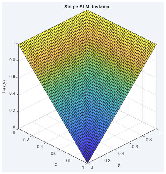
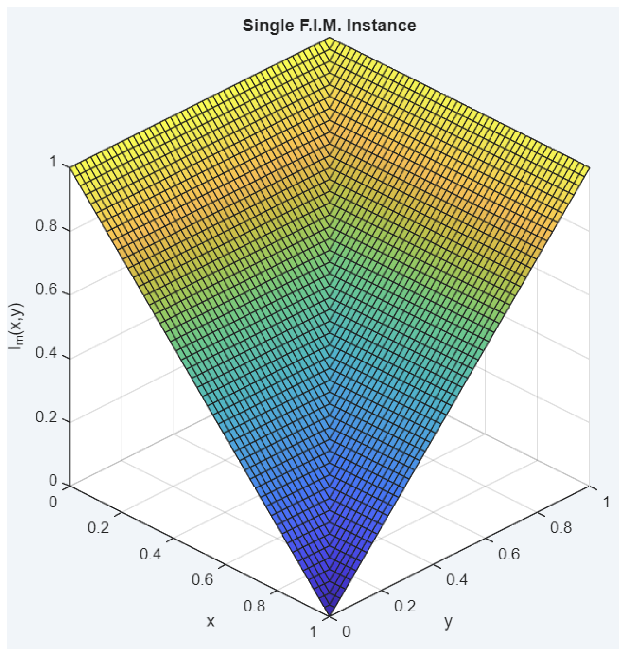
For illustration purposes, the graph of has been composed (see Figure 1), offering a visual confirmation of the results gathered above.
Figure 1.
Graph of and . The surface colour encodes the implication value and is used for visualisation purposes only.
Since and both reduce analytically to the Kleene–Dienes implication, their graphs coincide, and a single graphical verification suffices to confirm Proposition 3.
3.2. Discussion and Methodological Considerations
3.2.1. Positioning and Scope
The proposed Fuzzy Implication Modeling Theory targets specifically the subset of implications generated through compositions of the three basic fuzzy connectives: negation, conjunction, and disjunction. This framework is designed as a complement to, rather than a replacement for, existing class-level and family-level treatments of fuzzy implications. The theory addresses a structural gap in the literature—the absence of an intermediate organizational layer between the broad class-level classifications and the specific family-level constructs. Rather than superseding conventional approaches, it supplies vocabulary and analytical tools for the intermediate layer that have not previously been available within a unified formal framework.
3.2.2. Relation to Existing Classifications
Fuzzy Implication Models (F.I.M.s) and Fuzzy Implication Model Instances (F.I.M.I.s) occupy a novel position in the taxonomy of fuzzy operators. Unlike class-level descriptions (S-implications, R-implications, QL-implications, etc.) which characterize implications by their derivation principles, or family-level descriptions which group implications by parametric families, the F.I.M./F.I.M.I. framework organizes implications by their compositional structure. The three propositions formulated in this work—generation, traceability, and non-uniqueness—describe phenomena that cannot be expressed purely within a class-level or family-level formalism precisely because they refer to this intermediate compositional layer. For instance, the non-injective nature of the model-instance mapping (Proposition 3) reveals convergence patterns where structurally distinct compositions yield identical functional forms; this phenomenon is inaccessible to traditional approaches. Furthermore, the model-level quantitative descriptors (Behavior Index and Intra-Model Variability Index) enable quantitative comparisons across models and insights into compositional diversity that existing frameworks do not readily provide.
3.2.3. Choice of Central-Tendency and Dispersion Measures
The selection of the arithmetic mean and standard deviation as the basis for the Behavior Index and Intra-Model Variability Index reflects careful consideration of three guiding principles: alignment with the theory’s compositional semantics, consistency with the discretized sampling philosophy, and computational adaptability within automated frameworks. The arithmetic mean was chosen for the Behavior Index because it provides unbiased, neutral aggregation across all instances, is universally compatible with other statistical measures, and admits direct computational implementation. Standard deviation was chosen for the Intra-Model Variability Index because it directly measures dispersion and applies equal sensitivity to all deviations, and its square-root restoration to the original numerical scale preserves interpretability relative to both individual instances and the Behavior Index.
Alternative measures were rejected for principled reasons. The median paired with median absolute deviation (M.A.D.) would trade interpretability for robustness on the distribution’s tails; however, the discretized sampling already operates within the bounded domain without heavy-tailed phenomena, rendering the robustness gain marginal. A trimmed mean introduces an arbitrary trimming parameter that would compromise cross-model index comparability. The chosen measures thus balance theoretical coherence, computational efficiency, and the practical requirement that indices remain stable and comparable across different configurations of the depth and degree parameters k and n.
3.3. New Constructs
This subsection is dedicated to the detailed exposition of the above-mentioned concepts in strict mathematical terms. For clarity and illustration reasons, each construct has been assigned its own devoted sub-subsection where it will be discussed in detail.
3.3.1. F.I.M. Behavior Index
The introduction of the modeling aspect in fuzzy implications allows for a more organized and thorough study of their performance, properties and implementation in applications. However, as mentioned in the previous segment, one of the usual problems faced by researchers during the development of a fuzzy logic application related to implications is how to choose the appropriate one. In order to assist with this task, the authors propose the creation of a new construct, the Fuzzy Implication Model Behavior Index, which is defined as follows:
Definition 9.
The Behavior Index of a Fuzzy Implication Model is a matrix symbolized by with the formula:
Formula Description:
- is the Behavior Index Matrix. It summarizes on a grid the average behavior of a Fuzzy Implication Model through its instances.
- is an instance of the Fuzzy Implication Model, and the index j identifies which one.
- r is the index of the x-coordinate, ranging from 1 to k.
- s is the index of the y-coordinate, also ranging from 1 to k.
- is the number of sample points per axis (Index Depth), resulting in a matrix of size . NOTE: since otherwise the sampling procedure would be pointless.
- is the r-th sampled value on the x-axis. The sampled values are equally spaced in .
- is the s-th sampled value on the y-axis. The sampled values are equally spaced in .
- j is the index of the model’s instances, and it ranges from 1 to n.
- n is the total number of instances used in the Index (Index Degree).
Example 1
(Behavior Index of on two compositional instances). Throughout this example and Example 2, the designation “Gödel triple” is used to denote the pairing of the Gödel t-norm and t-conorm with the standard strong negation , rather than with the non-involutive Gödel negation of Gödel logic. The involutive choice is deliberate: with the standard strong negation, the composite reduces analytically to the Kleene–Dienes implication, a well-known classical implication that serves two distinct purposes here—as a familiar benchmark against which the reader can immediately cross-check the behavior of in this instance, and as the concrete reduction already invoked in the proof of Proposition 3, thereby tying Example 1 directly to the non-uniqueness property. Pairing the Gödel t-norm and t-conorm with the non-involutive Gödel negation would instead yield a closed-form reduction that lies outside the canonical set of named implications, forgoing both of these connections. Consider two compositional instances generated from : the first using the Gödel triple (, , ), which by direct substitution and the same simplification used in the proof of Proposition 3 reduces analytically to the Kleene–Dienes implication ; and the second using the Łukasiewicz triple (, , ). With discretization , the sampled points are and the two instances produce the following matrices (rows indexed by r, columns by s):
A natural question at this point is whether the Łukasiewicz triple, by analogy with the Gödel case above, yields an equally clean analytical reduction—specifically, to the classical Łukasiewicz implication . The answer is negative, and the reason is structural: the Gödel reduction to Kleene–Dienes relied on the idempotence , which cancels the inner term of and allows the outer composition to collapse. The Łukasiewicz t-norm, by contrast, is not idempotent: equals y only at the boundary values . The analogous simplification therefore cannot take place, and applied to the Łukasiewicz triple does not coincide with . Concretely, , whereas . This pointwise disagreement is not an isolated accident: it extends continuously to a subregion of on which saturates to 1 while does not. Its visual signature is the extended unit plateau covering the upper-right portion of Figure 2, on the coarse grid of Example 1; however, the two formulas happen to disagree only at the single cell computed above.
Figure 2.
Three-dimensional surface plot of the second instance (the Łukasiewicz-triple case). Connective selection: , , , feeding the same F.I.M. structure as in Figure 3. The surface colour encodes the implication value and is used for visualisation purposes only.
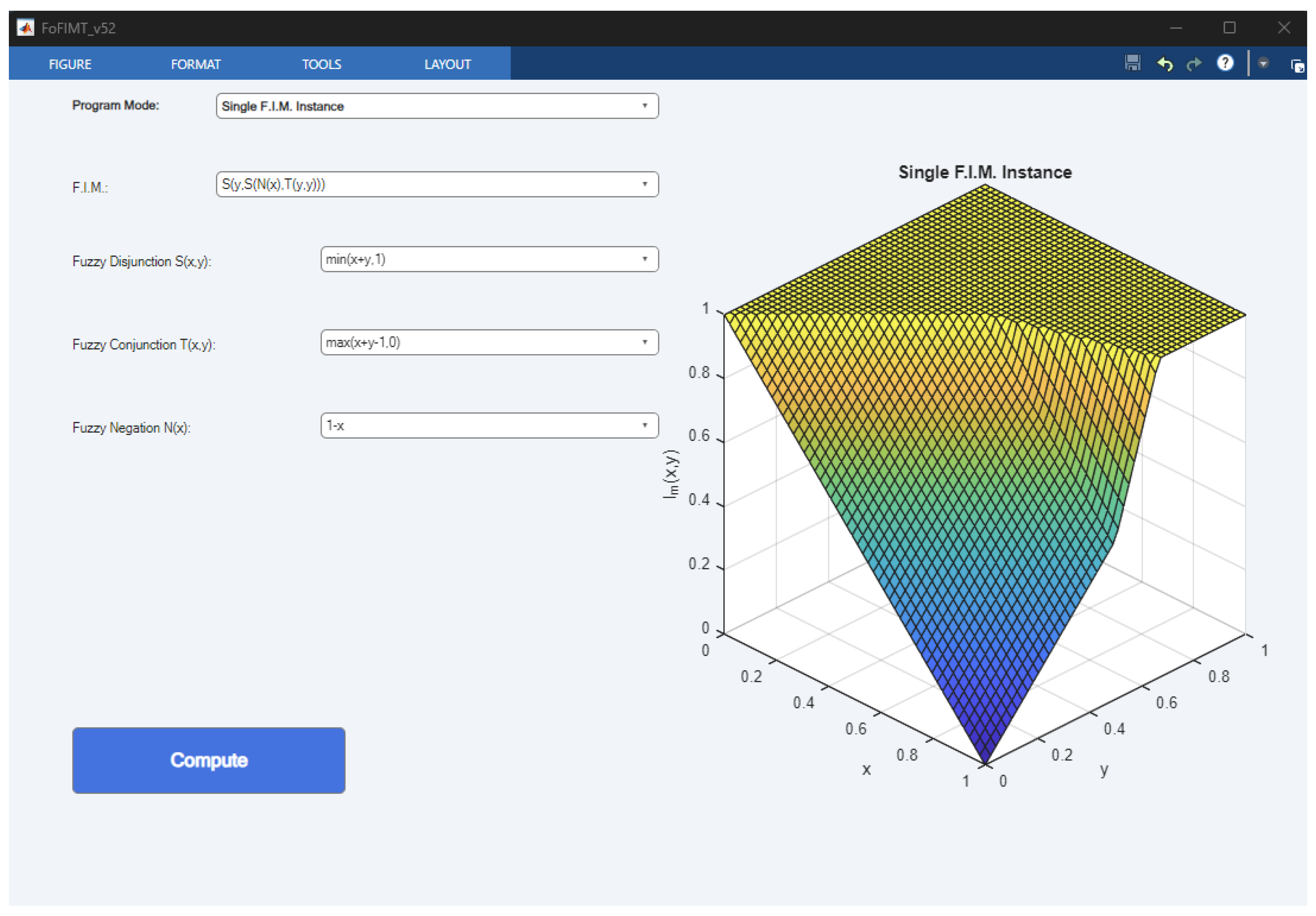
Figure 3.
Three-dimensional surface plot of the first instance (the Gödel/Kleene–Dienes case), produced by the companion MATLAB implementation. The panel on the left records the connective selection (, , ) feeding the F.I.M. structure ; the 3-D panel on the right displays the resulting surface over . The surface colour encodes the implication value and is used for visualisation purposes only.
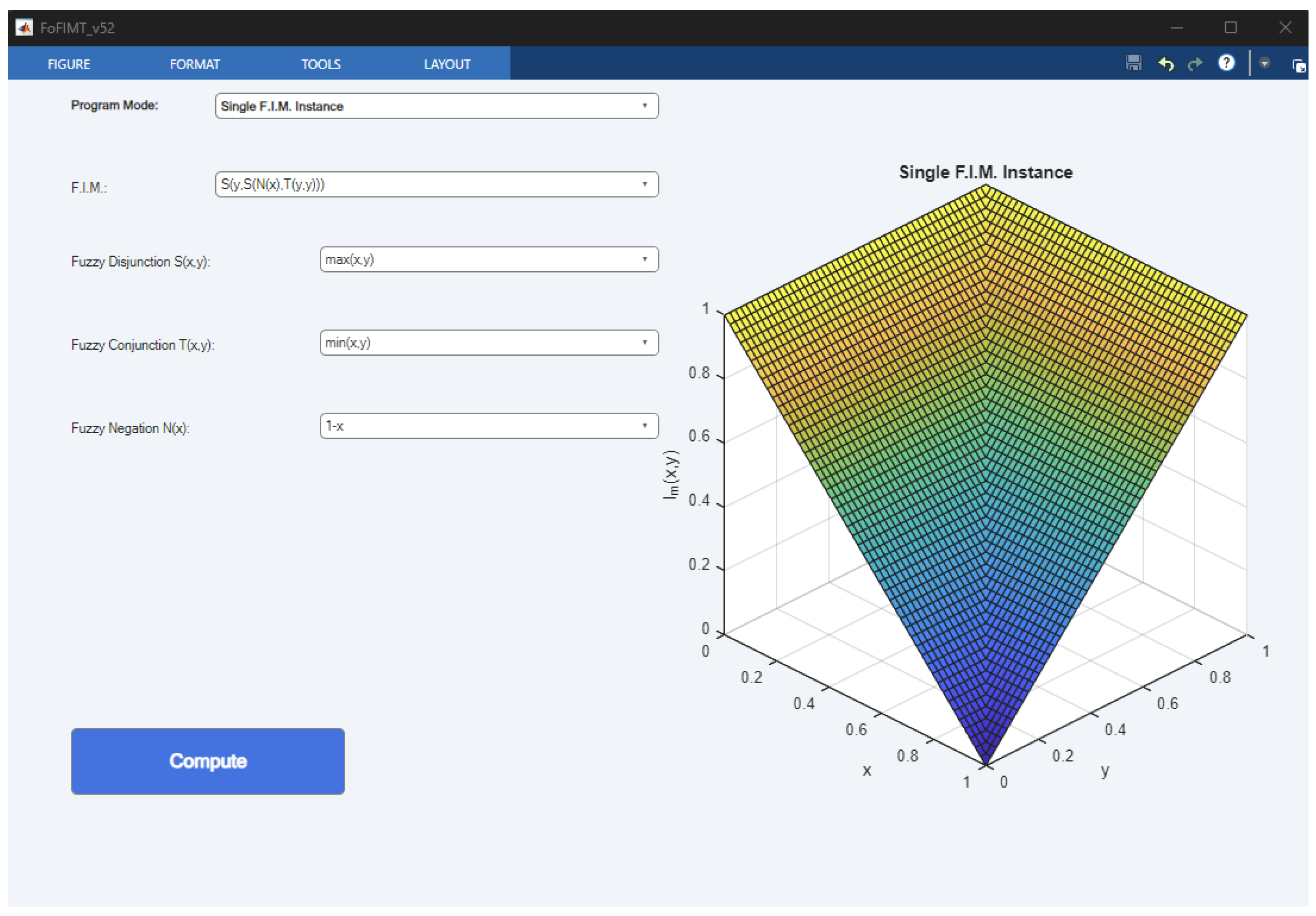
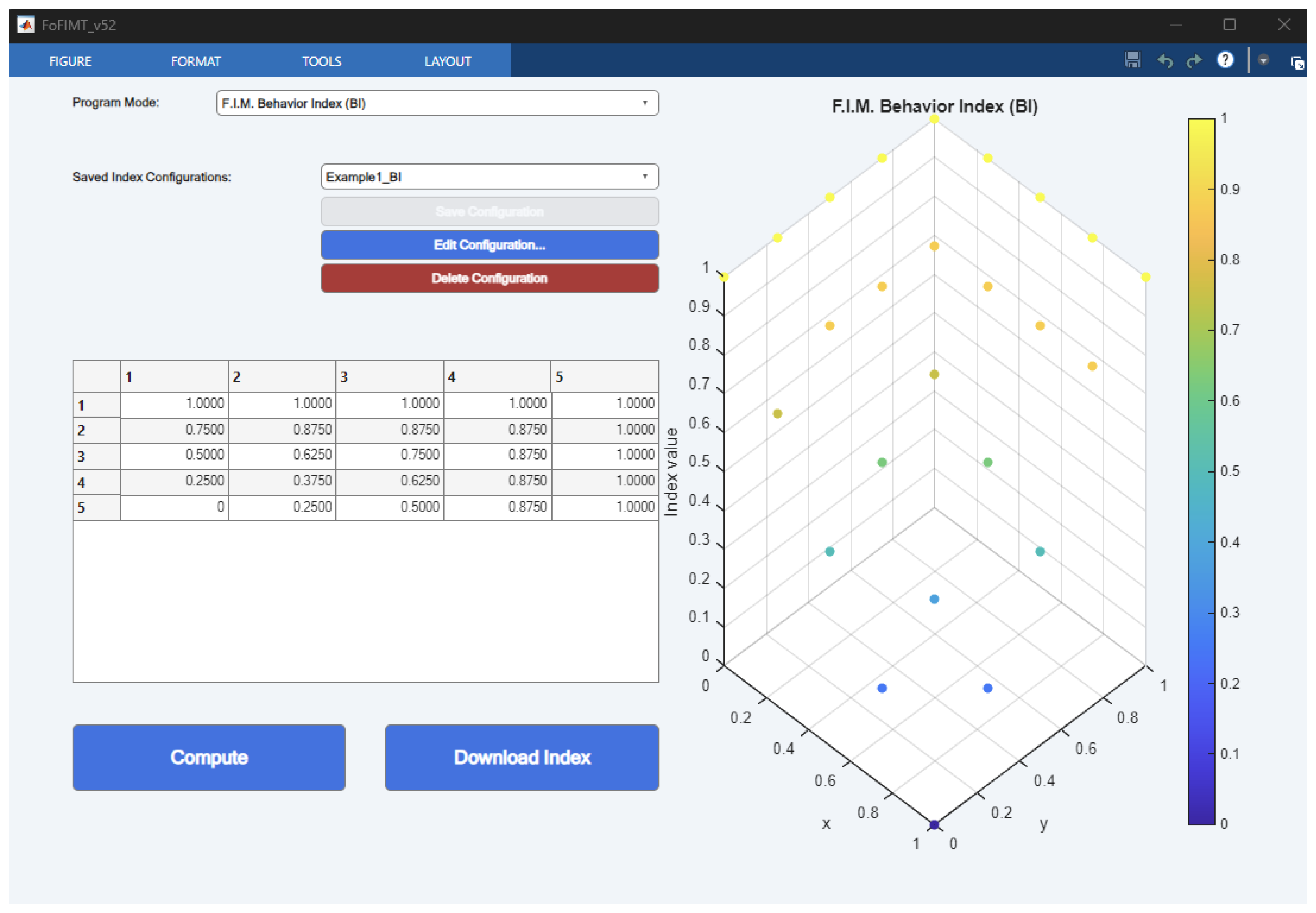
Consistent with the MATLAB realization described in Section 3.4, which stacks the instance surfaces into a three-dimensional array and aggregates them via pointwise mean along the instance axis, the Behavior Index of with is the pointwise average of the two matrices (see Figure 4):
Figure 4.
Behavior Index of produced by the companion MATLAB implementation from the two instances shown in Figure 2 and Figure 3, with Index Depth and Index Degree . The 3-D scatter plot on the right colors each grid point by its aggregated value; the numeric preview table on the left reproduces the matrix cell for the cell.
The aggregated behavior exhibits monotonicity decreasing in the antecedent and increasing in the consequent, with full activation along the top row () and along the right column (). The numerical mean of all entries is , which characterizes the model’s overall behavioral tendency as moderately affirmative. These same two instances are reused in the next sub-subsection, where they drive the Intra-Model Variability Index, providing a unified numerical image of both descriptors on a shared computational basis.
It is important to mention that each model has a single Behavior Index. However, due to Proposition 1, each model has an infinite number of instances making the definite calculation of the Index’s value practically impossible. For this reason, the concept is relying on two parameters (Index Attributes) k and n, named DEPTH and DEGREE accordingly, that independently regulate index accuracy.
NOTE: It can easily be understood that higher parameter values equal better results since a bigger degree will include more instances into the calculations while a bigger depth will provide a more dense index grid.
3.3.2. F.I.M. Intra-Model Variability Index
One more proposition aimed at assisting in the practical utilization of the paper’s research is the introduction of the Intra-Model Variability Index. The mentioned concept’s creation is directly aimed at addressing the importance of choosing the appropriate instance between the confinements of a single F.I.M. The definition of the described construct is the following:
Definition 10.
The Intra-Model Variability Index of a Fuzzy Implication Model is a matrix symbolized by with the formula:
Formula Description:
- is the Intra-Model Variability Index Matrix. It summarizes on a grid the intra-model variability of a Fuzzy Implication Model through its instances.
- is the Behavior Index of as it has been defined in Definition 9.
- is an instance of the Fuzzy Implication Model, and the index j identifies which one.
- r is the index of the x-coordinate, ranging from 1 to k.
- s is the index of the y-coordinate, also ranging from 1 to k.
- k is the number of sample points per axis (Index Depth), resulting in a matrix of size . NOTE: since otherwise the sampling procedure would be pointless.
- is the r-th sampled value on the x-axis. The sampled values are equally spaced in .
- is the s-th sampled value on the y-axis. The sampled values are equally spaced in .
- j is the index of the model’s instances, and it ranges from 1 to n.
- n is the total number of instances used in the Index (Index Degree).
Example 2
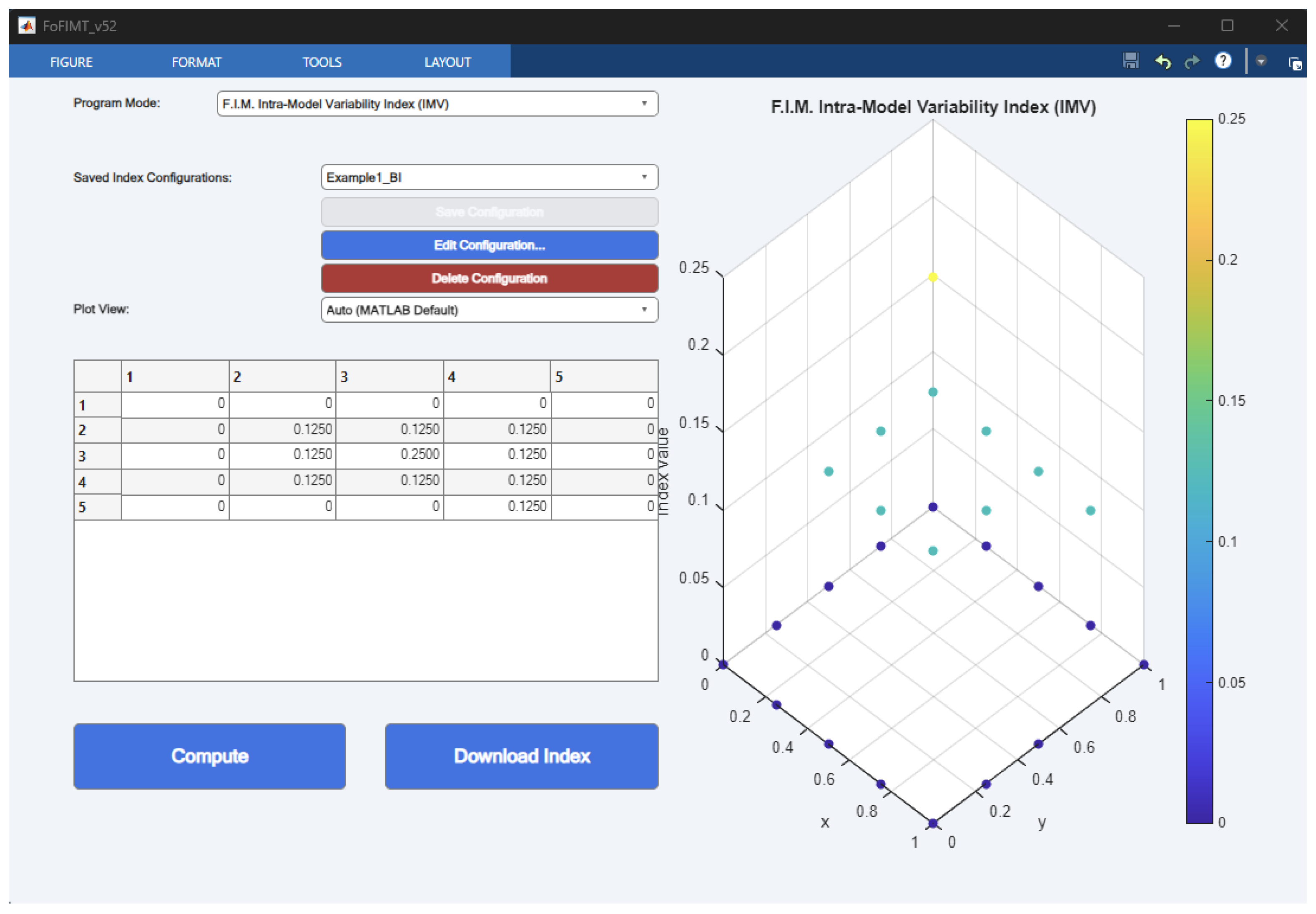
(Intra-Model Variability Index on the same two instances). Reusing the two instances introduced in Example 1 (the Gödel triple and the Łukasiewicz triple, both with standard negation ), and the Behavior Index already obtained as their pointwise mean with aggregate value , the Intra-Model Variability Index measures how much each instance deviates from this average at each grid point:
with mean . The variability is null on the boundaries , and where both instances coincide, and peaks at where the two connective choices diverge most (see Figure 5). The small numerical magnitude of the IMV entries indicates that, on this coarse grid, the two connective pairs produce broadly similar implications even though they are structurally distinct; an IMV with uniformly low values would suggest that instance selection is largely inconsequential, whereas higher variability would reveal strong sensitivity to the t-norm/t-conorm choice.
Figure 5.
Intra-Model Variability Index of on the same two instances and configuration as in Figure 4 (Index Depth , Index Degree ). The interior peak at and the null boundary along , , are clearly visible; the preview table on the left reproduces the matrix cell for the cell.
As with the Behavior Index, each model has a single Intra-Model Variability Index, but its definite calculation is practically impossible due to the infinite number of instances (Proposition 1). The same two Index Attributes (DEPTH k and DEGREE n) regulate accuracy in an identical manner. It should be noted that the divisor n is used in the formula rather than because the n instances constitute the complete reference set for a given index configuration, not a random sample drawn from a larger population.
3.3.3. Index Attribute Manipulation
The two indexes introduced in the current paper, despite their theoretical abstraction, have been formulated with practicality in mind, a fact reflected in the use of the two Index Attributes in both concept definitions. To elaborate, these parameters were initially introduced as a mechanism of “scaling” the index definitions down in a form that can be easier automated without sacrificing conceptual sophistication. However, their integration proved more valuable than initially expected, since it rendered possible a plethora of novel and unconventional uses for the indicators providing an added layer of flexibility.
Taking the above into consideration, setting the degree attribute n to an unconventionally low value (e.g., 2, 3, …) fundamentally alters its interpretation. This statement is directly correlated to the ’s and ’s particularity of depending on high index attributes in order to properly represent their true theoretical center. As a result, a side effect of this circumstance is the significant divergence of each concept’s symbolism the lower n gets into the single digit range. Nevertheless, in cases where something like this occurs, the index scope shifts from the model to the sub-model level.
On the other hand, the manipulation of the depth attribute of the behavior index k seems to not offer any theoretical insight in relation to either of the indicators. This observation, however, is not concerning, given that its modification can still significantly impact the metrics in a different way. To elaborate, even though the limitation of the attribute to lower values may hinder the index’s ability to fulfill its initial mission, it presents substantial computational savings through the influence it exerts over the computations each index calculation demands (the number of evaluation points for any given index configuration are ). As a result, it can easily be understood that restricting k to generally low values can lead to a significant decrease in processing power. To put it another way, the ability to downsize the depth attribute offers researchers the choice of balancing between achieving their objective and limiting computational waste by adapting index precision.
In addition, it has to be highlighted that the capability of altering both index attributes independently renders the indexes under their combined influence. So, given that n and k share the same parameter values where indicator dynamics change, Table 1 has been created in order to present in an orderly way the combined effect of their alteration. It is worth noting that the impact of attribute manipulation is identical for both and .
Table 1.
Index attribute manipulation impact on and .
In view of the aforementioned points, it easily becomes apparent that a researcher can, through attribute manipulation, both re-purpose the indicators in order to fit the scope of problems they were not explicitly designed to address, and/or at the same time, address one of their prevalent shortcomings.
3.4. Computational Realization
The framework has been implemented as a MATLAB R2025b companion tool with a graphical user interface, designed for reproducibility and pedagogical exploration. The program is self-contained, requiring no external libraries beyond MATLAB’s core toolboxes, and is freely available at the paper’s repository [25].
The tool operates in four modes: (1) Single F.I.M. Instance evaluation, allowing users to select a model, specify connectives, and visualize a custom instance; (2) Behavior Index computation, enabling calculation of the model-level aggregate matrix with configurable depth and degree parameters; (3) Intra-Model Variability visualization, supporting both -normalized and auto-scaled plot views; and (4) F.I.M. Designer, an interactive tree-based environment for composing new models from the three basic connectives, with real-time mathematical formula display and model persistence.
The F.I.M. Designer represents the tool’s principal innovation. It provides a graphical canvas for constructing implication trees, a Formula Preview panel that updates symbolically as the structure evolves, and an Actions module for model validation, duplication detection, and lifecycle management. Users interact via direct mouse selection or keyboard shortcuts, and the interface enforces arity constraints to maintain well-formedness at all times.
Computational realization employs MATLAB function handles for operator representation, nested functional calls for compositional evaluation, co-domain clipping for numerical stability, parameter propagation for parametric families, and discretized sampling for index computation. A three-dimensional array structure aggregates implication surfaces across instances, enabling efficient pointwise averaging and dispersion calculation. All evaluation is numerical rather than symbolic, trading algebraic completeness for responsiveness and scalability on standard computational platforms.
Full UI walkthroughs, execution instructions, and mode-by-mode screenshots are provided in the Supplementary Materials accompanying this paper.
4. Results and Discussion
The analytical development and computational realization of the proposed theoretical framework yielded structural, quantitative, and computational results. The principal findings are examined in the following subsections.
4.1. Structural Organization of the Implication Space
The proposed framework establishes that the subclass of fuzzy implication functions generated through compositions of basic fuzzy logical connectives admits a two-level structural organization. At the first level, Fuzzy Implication Models (F.I.M.s) operate as connective-level compositional templates, while at the second level, Fuzzy Implication Model Instances (F.I.M.I.s) correspond to the fully specified implication functions obtained via connective substitution.
The three structural propositions formulated in this work reveal specific properties of the model–instance relationship. In particular, each model admits an infinite instance generation capacity through the use of parametric connectives (Proposition 1), every instance maintains guaranteed association with at least one admissible model (Proposition 2), and the mapping between models and instances is non-injective, as demonstrated through the convergence of structurally distinct compositions to identical functional forms (Proposition 3). Furthermore, the validity of the proposed model was established through a complete verification of the standard implication conditions –.
Discussion. These findings reinforce a connective-centered structural interpretation that extends conventional treatments of fuzzy implications as standalone operators. The explicit model–instance separation clarifies structural relationships governing implication generation, reduction mechanisms, and equivalence patterns.
In particular, the non-injective nature of the mapping provides a theoretical explanation for convergence phenomena observed in implication constructions, where structurally distinct connective compositions reduce to identical functional forms. This observation carries practical significance, as it indicates that the effective number of distinct implications within any given model may be substantially smaller than the combinatorial space of connective substitutions would suggest.
4.2. Behavioral Quantification and Discretization Effects
The application of the Behavior Index () and the Intra-Model Variability Index () to the proposed model demonstrates that the two constructs successfully capture complementary aspects of model-level behavior. The produces a discretized approximation of the average functional behavior induced by a model across its instances, while the quantifies the degree of behavioral dispersion among those instances, thereby distinguishing between behaviorally coherent models and those exhibiting significant instance-dependent deviations.
Furthermore, the analysis of the discretization parameters reveals that sampling depth (k) and instance degree (n) induce distinct interpretative regimes. At high values, both indexes converge toward their theoretical targets at the model level. At low values of n, the scope shifts from model-level characterization to sub-model analysis, while low values of k reduce computational cost at the expense of grid resolution.
Discussion. From a behavioral standpoint, the construct extends analysis beyond the level of isolated implication functions by representing models as aggregated behavioral entities. This shift enables quantitative comparison between models and clarifies how connective compositions influence global implication characteristics.
The formulation introduces a diagnostic perspective on model robustness. Low variability indicates behavioral stability across instances, whereas elevated dispersion reveals structural sensitivity to connective substitution. The index therefore provides insight into the internal behavioral coherence of Fuzzy Implication Models.
The discretization-dependent regimes establish a controlled trade-off between approximation fidelity and computational complexity, offering researchers the flexibility to balance precision against efficiency depending on the analytical objective.
Finally, the aggregation framework enables the definition of a Representative Implication, interpreted as an interpolative approximation of aggregated model behavior. This construct introduces an additional abstraction layer linking models with characteristic functional representatives. Theoretical properties of such representatives, particularly with respect to preservation of the standard implication conditions under interpolation, remain open for further analytical investigation.
4.3. Computational Operationalization and Analytical Exploration
The theoretical constructs developed in this work admit a stable numerical realization, implemented through a MATLAB-based program, that preserves the functional structure of connective compositions under discretized evaluation. The function-handle encoding strategy enables the substitution of arbitrary connective triplets within an invariant computational pipeline, while nested functional calls preserve the hierarchical dependency structure of model compositions. The implementation successfully supports the computation of both indexes across varying parameter configurations, the interactive construction of new models through the F.I.M. Designer, and the visualization of implication surfaces, aggregation profiles, and variability patterns.
Discussion. The numerical operationalization demonstrates the computational feasibility of the framework while supporting controlled evaluation of model-level behaviors. The ability to explore implication instances, behavioral indices, and variability patterns through a graphical user interface establishes a practical bridge between abstract theoretical constructs and empirical analysis, rendering the framework accessible to researchers regardless of their programming proficiency. Additionally, graphical inspection enhances interpretability, facilitates comparative evaluation across different connective configurations, and strengthens experimental transparency. The extensible architecture of the program further supports the integration of additional models and connectives in future investigations.
4.4. Limitations and Future Research Directions
Despite the structural consistency and computational feasibility demonstrated by the proposed framework, certain limitations must be acknowledged. These limitations do not undermine the validity of the formulation but rather delineate the conditions under which the present analysis operates and highlight opportunities for further refinement.
First, the framework relies on discretized sampling strategies for behavioral approximation. As a result, approximation fidelity depends on grid resolution and instance selection policies. Second, the formal properties of derived constructs, including Representative Implications, require further analytical investigation, particularly with respect to the preservation of implication axioms.
In light of these considerations, several directions for future research naturally emerge:
4.4.1. Representative Implication
After evaluating in a broader spectrum, it becomes apparent that it can be utilized in the formulation of a new, inherently more complex concept. Consequently, the current sub-subsection has been formulated with the purpose of presenting the construct in question, which in essence refers to a new category of fuzzy implications. To elaborate, the present segment will mainly focus on the foundational principles of the novel implications, as well as on outlining their distinctive features.
According to the definition (see Definition 9), the index is essentially a two-dimensional matrix that approximates the model’s average behavior. However, a different concept interpretation would indicate its alternative status as a fuzzy truth table of a yet-to-be-defined fuzzy implication. The implication in question would be the result of an interpolation process applied to the index, with the added limitations of retaining certain data trends, like monotonicity, that are instrumental for the categorization of the produced formula as a fuzzy implication. Furthermore, it has to be highlighted that the final function will inherit the index’s primary role, resulting in a formula that approximates the average instance of a given model.
Taking the above into consideration, a promising interpolation method would be an implementation of a form of two-dimensional interpolation like Tensor-product Piecewise Cubic Hermite Interpolation (P.C.H.I.P.). However, carrying out such a deep dive into the concept within the limits of the current paper would shift its theoretical center away from what the article’s authors initially intended. So, the evolution of the concept will not be pursued any further here and instead, the discovery of the instance’s formula and the validation of its property as a fuzzy implication are labeled as open problems with the hope that they will be addressed in the future.
NOTE: Given that the concept of the Representative Implication is heavily dependent on the Behavior Index, it is impacted similarly when subject to attribute manipulation (see Table 1).
4.4.2. Algorithmic Framework for Selecting the Fuzzy Implication That Best Reflects a Given Logical Relationship
A persistent challenge in fuzzy logic applications concerns the selection of an implication that best describes a given logical connection. Despite the importance of this problem, no field-wide practice has been developed to address it within fuzzy logic, with relevant studies resorting to external methods such as statistics to approximate a solution [26].
The concepts introduced by Fuzzy Implication Modeling theory enable the formulation of a novel selection strategy that operates within the confines of the framework. The procedure begins with the researcher specifying a desired implication profile, which forms the Requirement Set. All established F.I.M.s are then identified, and for each, the Behavior Index is calculated. Each model is evaluated against the Requirement Set: if it matches the intended profile, it is accepted; otherwise, the evaluation proceeds to the next F.I.M. If no models remain, the researcher is encouraged to revise the intended profile.
Upon acceptance of a model, the researcher may either select its Representative Implication or conduct further analysis in the intra-model space. The Intra-Model Variability Index determines whether further analysis is necessary: low variability suggests that instance selection within the model is inconsequential, while significant dispersion prompts the division of instances into smaller groups (Sub-Models). The Behavior Index is then recalculated for each Sub-Model and evaluated against the Requirement Set. If no suitable Sub-Model is found, the researcher is directed to a different F.I.M. When a Sub-Model is selected but still exhibits high variability, the algorithm concludes that further searching is not viable and redirects the analysis accordingly.
It is important to clarify the scope of this section: the primary objective is to establish the general outline of a promising future research route, rather than to present a fully operational methodology. The methodology is not complete and cannot be directly applied as it stands, since a comprehensive development of all of its concepts would shift the paper’s theoretical center away from its intended scope. The algorithm above references three constructs that are intentionally left as conceptual placeholders: Requirement Sets and Sub-Models have not been formally defined in this work, and Representative Implications rest on an interpolation process whose closed-form expression and whose preservation of the fuzzy-implication conditions are open problems (see Section 4.4.1). Their presence in the algorithmic description above should therefore be read as structural scaffolding rather than as formal operators of the framework. This is an intentional choice aimed at capturing the conceptual structure of the approach without premature formalization.
For the same reason, no worked numerical instantiation of the algorithm is provided in this work. The authors considered supplying such an instantiation during the present revision and concluded that, at this stage of development, it would not be scientifically sound: running the algorithm to completion requires fixing particular interpretations of the three placeholders above, which either (i) implicitly commits the paper to definitions of those constructs that it has not derived—extending the scope of the work beyond what is argued—or (ii) produces a demonstration whose conclusions pertain to the chosen assumptions rather than to the framework itself, since those assumptions are not theorems of this paper. Accordingly, the present sub-subsection is kept at the conceptual level, and concrete instantiations are deferred to future work in which the three open constructs have first been formally developed.
The algorithmic procedure has been represented as a flowchart composed through “draw.io” and exported as an interactive HTML file, available at the paper’s open repository [25]. Concrete applied research directions that presuppose the future development of the three open constructs are listed in the sub-subsection that follows.
4.4.3. Additional Future Research Directions
Beyond the above, additional directions for future research include:
- Investigation of alternative aggregation and dispersion operators.
- Extension of the proposed framework with the inclusion of more fuzzy implication families, and/or classes of fuzzy connectives.
- Discovery of more Fuzzy Implication Models.
- Empirical benchmarking of and other instances of the proposed framework against classical implications in representative fuzzy inference systems (e.g., Mamdani-style controllers on standard benchmark problems), quantifying accuracy, convergence and computational cost.
- Use of the Behavior Index as a principled selection criterion in rule-based design, with a case study on an applied domain such as medical decision support or process control.
- Integration of the F.I.M. Designer module into an open educational platform for teaching fuzzy logic, with accompanying empirical studies on pedagogical effectiveness.
5. Conclusions
The present study introduced a structured theoretical framework for the analysis and organization of fuzzy implication functions generated through compositions of basic fuzzy logical connectives. In particular, the formulation established a connective-centered modeling perspective supported by the differentiation between Fuzzy Implication Models (F.I.M.s) and Fuzzy Implication Model Instances (F.I.M.I.s), together with a formal characterization of their relational properties through three structural propositions.
Furthermore, the definition of the Behavior Index () and the Intra-Model Variability Index () enabled quantitative behavioral characterization at the model level, thereby extending implication analysis beyond individual functional instances. In parallel, the computational operationalization of the theoretical constructs through a dedicated MATLAB-based program demonstrated numerical feasibility and supported systematic behavioral exploration.
Taken together, these findings indicate that the integration of structural modeling, behavioral quantification, and computational realization can provide a coherent and analytically robust foundation for implication-centered fuzzy logic analysis, even though the framework relies on constructs whose properties warrant further research.
In this regard, future research may address the discovery of additional fuzzy implication models, the formal characterization of representative implications, the development of alternative aggregation mechanisms, and the further refinement of the algorithmic framework for fuzzy implication selection.
Supplementary Materials
The following supporting information can be downloaded at https://www.mdpi.com/article/10.3390/axioms15050348/s1: Section S1—Execution Instructions for the F.I.M. Designer companion program; Section S2—User Interface and Usability, with mode-by-mode screenshots of the Single-Instance, Behavior Index, Intra-Model Variability Index, and Designer modes (Figures S1–S9); Section S3—Code Readability and Modification; Section S4—Computational Realization (Detailed), covering the encoding of fuzzy logical connectives, direct realization of implication compositions, co-domain enforcement and numerical stability, propagation of operator parameters, graphical visualization mechanisms, extensibility, the distinction between numerical and symbolic realization, handling of the Behavior and Variability indices, F.I.M. Designer structural composition, and persistence mechanisms.
Author Contributions
Conceptualization, E.M. and S.M.; methodology, E.M. and S.M.; software, E.M.; validation, A.K.; investigation, E.M. and S.M.; writing—original draft preparation, E.M. and S.M.; writing—review and editing, E.M., S.M. and A.K.; visualization, E.M.; supervision, A.K. and B.K.P.; project administration, A.K.; and funding acquisition, A.K. All authors have read and agreed to the published version of the manuscript.
Funding
This research work was funded by the Special Account for Research Funds of Democritus University of Thrace (D.U.T.H.) under project code 83136; the APC was funded from the same account.
Data Availability Statement
The source code of the MATLAB program developed in this study is openly available at [25].
Conflicts of Interest
The authors declare no conflicts of interest.
Abbreviations
The following abbreviations are used in this manuscript:
| F.I.M. | Fuzzy Implication Model |
| F.I.M.I. | Fuzzy Implication Model Instance |
| B.I. | Behavior Index |
| I.M.V. | Intra-Model Variability Index |
| M.A.D. | Median Absolute Deviation |
| P.C.H.I.P. | Piecewise Cubic Hermite Interpolating Polynomial |
| A.S.T. | Abstract Syntax Tree |
| G.U.I. | Graphical User Interface |
References
- Precup, R.E.; Hellendoorn, H. A survey on industrial applications of fuzzy control. Comput. Ind. 2011, 62, 213–226. [Google Scholar] [CrossRef] [Scilit]
- Sinha, M.; Tiwari, R. A Comprehensive Survey of Fuzzy Logic Utilization in Different Agricultural Sectors. J. Stat. Math. Eng. 2024, 10, 1–7. [Google Scholar] [CrossRef] [Scilit]
- Makariadis, S.; Papadopoulos, B. A Fuzzy Implication-Based Approach for Validating Climatic Teleconnections. Mathematics 2022, 10, 2692. [Google Scholar] [CrossRef] [Scilit]
- Makariadis, S.; Makariadis, E.; Konguetsof, A.; Papadopoulos, B. New Fuzzy Implication Model Consisting Only of Basic Logical Fuzzy Connectives. Axioms 2024, 13, 777. [Google Scholar] [CrossRef] [Scilit]
- Kacprzyk, J.; Yager, R.R. (Eds.) Management Decision Support Systems Using Fuzzy Sets and Possibility Theory; Number 83 in Interdisciplinary systems research; Verlag TÜV Rheinland: Köln, Germany, 1985. [Google Scholar]
- Mas, M.; Monserrat, M.; Torrens, J. QL-implications versus D-implications. Kybernetika 2006, 42, 351–366. [Google Scholar]
- Yager, R.R. On some new classes of implication operators and their role in approximate reasoning. Inf. Sci. 2004, 167, 193–216. [Google Scholar] [CrossRef] [Scilit]
- Baczyński, M.; Jayaram, B. Fuzzy Implications from Fuzzy Logic Operations. In Fuzzy Implications; Springer: Berlin/Heidelberg, Germany, 2008; pp. 39–107. [Google Scholar] [CrossRef] [Scilit]
- Massanet, S.; Riera, J.V.; Ruiz-Aguilera, D. On Fuzzy Polynomial Implications. In Information Processing and Management of Uncertainty in Knowledge-Based Systems; Laurent, A., Strauss, O., Bouchon-Meunier, B., Yager, R.R., Eds.; Springer International Publishing: Cham, Switzerland, 2014; pp. 138–147. [Google Scholar]
- Massanet, S.; Mir, A.; Riera, J.V.; Ruiz-Aguilera, D. Fuzzy implication functions with a specific expression: The polynomial case. Fuzzy Sets Syst. 2022, 451, 176–195. [Google Scholar] [CrossRef] [Scilit]
- Vemuri, N.R. Investigations of fuzzy implications satisfying generalized hypothetical syllogism. Fuzzy Sets Syst. 2017, 323, 117–137. [Google Scholar] [CrossRef] [Scilit]
- Kurková, V.; Manolopoulos, Y.; Hammer, B.; Iliadis, L.S.; Maglogiannis, I. (Eds.) Artificial Neural Networks and Machine Learning—ICANN 2018—27th International Conference on Artificial Neural Networks, Rhodes, Greece, 4–7 October 2018, Proceedings, Part I; Lecture Notes in Computer Science; Springer: Berlin/Heidelberg, Germany, 2018; Volume 11139. [Google Scholar] [CrossRef] [Scilit]
- Jayaram, B.; Mesiar, R. On special fuzzy implications. Fuzzy Sets Syst. 2009, 160, 2063–2085. [Google Scholar] [CrossRef] [Scilit]
- Shi, Y.; Van Gasse, B.; Ruan, D.; Kerre, E. On a New Class of Implications in Fuzzy Logic. In Information Processing and Management of Uncertainty in Knowledge-Based Systems Theory and Methods; Hullermeier, E., Kruse, R., Hoffmann, F., Eds.; Communications in Computer and Information Science; Springer: Berlin/Heidelberg, Germany, 2010; Volume 80, pp. 525–534. [Google Scholar] [CrossRef] [Scilit]
- Baczyński, M.; Jayaram, B. Fuzzy Implications. In Studies in Fuzziness and Soft Computing; Springer: Berlin/Heidelberg, Germany, 2008; Volume 231. [Google Scholar]
- Shi, Y. A Deep Study of Fuzzy Implications. Ph.D. Thesis, Ghent University, Ghent, Belgium, 2009. [Google Scholar]
- Fodor, J. On fuzzy implication operators. Fuzzy Sets Syst. 1991, 42, 93–300. [Google Scholar] [CrossRef] [Scilit]
- Bedregal, B. On Fuzzy Negations and Automorphisms. An. CNMAC 1984, 2, 1127–1129. [Google Scholar]
- Fodor, J.; Roubens, M. Fuzzy Preference Modelling and Multicriteria Decision Support. In Theory and Decision Library, Serie D: System Theory, Knowledge Engineering and Problem Solving; Kluwer Academic Publishers: Dordrecht, The Netherlands, 1994; Volume 14, pp. 3–16. [Google Scholar]
- Gottwald, S. A Treatise on Many-Valued Logics; Research Studies Press: Baldock, UK, 2001; pp. 63–105. [Google Scholar]
- Weber, S. A General Concept of Fuzzy Connectives, Negations and Implications Based on T-Norms and T-Conorms on the representation of fuzzy rules. Fuzzy Sets Syst. 1983, 11, 115–134. [Google Scholar]
- Trillas, E. Sobre funciones de negacin en la teora de conjuntos difusos. Stochastica 1979, III, 47–60. (In Spanish) [Google Scholar]
- Klement, E.; Mesiar, R.; Pap, E. Triangular Norms; Kluwer: Dordrecht, The Netherlands, 2000; pp. 4–10, 108–110. [Google Scholar]
- Casella, G.; Berger, R.L. Statistical Inference, 2nd ed.; Duxbury/Thomson Learning: Pacific Grove, CA, USA, 2002. [Google Scholar]
- Makariadis, E. Formulation of the Fuzzy Implication Modeling Theory. 2026. Available online: https://github.com/Eleftherios-Makariadis/Formulation_of_the_Fuzzy_Implication_Modeling_Theory (accessed on 3 May 2026).
- Ellina, G.; Papaschinopoulos, G.; Papadopoulos, B.K. Fuzzy Inference Systems: Selection of the most Appropriate Fuzzy Implication from Available Lake Water Quality Statistical Data. Environ. Process. 2017, 4, 923–935. [Google Scholar] [CrossRef] [Scilit]

Disclaimer/Publisher’s Note: The statements, opinions and data contained in all publications are solely those of the individual author(s) and contributor(s) and not of MDPI and/or the editor(s). MDPI and/or the editor(s) disclaim responsibility for any injury to people or property resulting from any ideas, methods, instructions or products referred to in the content. |
© 2026 by the authors. Licensee MDPI, Basel, Switzerland. This article is an open access article distributed under the terms and conditions of the Creative Commons Attribution (CC BY) license.