Geometric and Algebraic Characterizations of Infeasibility of Rank Reversal in the Saaty and Belton–Gear Frameworks

Abstract

We investigate the infeasibility of rank reversal in the Analytic Hierarchy Process under the Saaty and Belton–Gear frameworks. In the Saaty framework, we propose an algebraic characterization and show that it is equivalent to the geometric characterization in previous studies. We then extend both characterizations to the Belton–Gear framework and prove that the infeasibility of rank reversal is identical across the two frameworks. Our analysis further reveals that the feasibility of rank reversal is an intrinsic property of the original matrix, whereas its realization additionally depends on the introduced option, thereby reconciling seemingly contradictory findings reported in the literature. Several examples are provided to illustrate the theoretical results.

1. Introduction

The Analytic Hierarchy Process (AHP), introduced by Saaty [1,2,3], is one of the most widely used tools in Multi-Criteria Decision Making (MCDM) [4]. Its pairwise comparison framework and hierarchical structure have attracted an enormous amount of interest from both researchers and practitioners in various fields, including industrial engineering, supply chain management, environmental planning, and so on [5,6,7].

The AHP has been subject to ongoing debate regarding the rank reversal phenomenon [8,9]. Rank reversal occurs when the relative ranking of existing options changes after a new option is introduced into the option set [10]. This issue has sparked considerable controversy and has led to numerous investigations [10,11,12,13,14,15,16,17,18,19,20,21,22].

Belton and Gear [10] provide the first instance of rank reversal in the AHP literature and propose a modification to the standard Saaty framework. Their framework suggests that priorities should be normalized by the maximum. However, Saaty and Vargas [11] respond with a counter-example, which demonstrates that the Belton–Gear normalization does not entirely eliminate rank reversal. Krause and Köppel [23] and Qiu et al. [24] have further emphasized the practical implications of rank instability. Peng et al. [25] provide a comprehensive discussion demonstrating that the modified Belton–Gear normalization [12] remains susceptible to rank reversal. More recently, Yan and Mao [26] established an infeasibility condition for rank reversal in the standard Saaty AHP framework.

Building upon Yan and Mao [26], our primary contributions are as follows:

• Proposing an algebraic approach towards the infeasibility of rank reversal in the Saaty framework;
• Establishing the equivalence between the geometric approach and the algebraic approach in the Saaty framework;
• Extending both the geometric approach and the algebraic approach from the Saaty framework to the Belton–Gear framework;
• Establishing the equivalence between the infeasibility of rank reversal in the Saaty framework and that in the Belton–Gear framework.

Our analysis reveals a crucial distinction between the feasibility of rank reversal and its realization. In particular, our results show that the feasibility of rank reversal is an intrinsic property of the original matrix, whereas its realization depends additionally on the added option. This finding reconciles seemingly contradictory claims in the literature [10,11]: both the Saaty framework and the Belton–Gear framework may prevent rank reversal in some instances, while permitting it in others.

The remainder of this paper is organized as follows. Section 2 reviews the Saaty framework and the infeasibility conditions developed by Yan and Mao [26] and presents both geometric and algebraic formulations. Section 3 introduces the Belton–Gear framework and extends the infeasibility analysis in the Belton–Gear framework. Section 4 presents detailed illustrations using multiple examples. Section 5 concludes with a discussion of the theoretical implications and directions for future research. Proofs of all theorems are collected in Appendix A.

2. The Saaty Framework

2.1. Preliminaries

Consider a set $\mathcal{Q}={\left\{x_i\right\}}_{i=1}^n$ of $n⩾2$ options and a set of m criteria indexed by $\ell =1$, 2, …, $m⩾2$. Under the criterion ℓ, there is a pairwise comparison matrix $A_{\ell }$, which is assumed to be cardinally consistent here, and can yield a vector ${\mathit{w}}_{\ell }$ of priorities, where

$$\begin{array}{cc}\hfill A_{\ell }& =\left(\begin{array}{cccc}{a}_{11|\ell }& a_{12|\ell }& \dots & a_{1n|\ell }\\ a_{21|\ell }& a_{22|\ell }& \dots & a_{2n|\ell }\\ ⋮& ⋮& \ddots & ⋮\\ a_{n1|\ell }& a_{n2|\ell }& \dots & a_{nn|\ell }\end{array}\right),\hfill \end{array}$$

(1)

$$\begin{array}{cc}\hfill {\mathit{w}}_{\ell }& ={(w_{\ell }(x_1,\mathcal{Q}),w_{\ell }(x_2,\mathcal{Q}),\dots ,w_{\ell }(x_n,\mathcal{Q}))}^{\top }.\hfill \end{array}$$

(2)

Note that $a_{ij|\ell }=w_{\ell }(x_i,\mathcal{Q})/w_{\ell }(x_j,\mathcal{Q})$. The cardinal consistency demands that

$$a_{ik|\ell }=a_{ij|\ell }{a}_{jk|\ell },1⩽i,j,k⩽n.$$

We point out that the cardinal consistency of $A_{\ell }$ is crucial for our further investigation. Although cardinally inconsistent matrices are ubiquitous in real world applications, our focus on cardinally consistent matrices is still valuable because it is fundamental to the understanding of AHP and can be viewed as a springboard for prospective investigation on the inconsistent case.

Note that $w_{\ell }(x_i,\mathcal{Q})\in (0,1)$, $1⩽i⩽n$, and ${\sum }_{i=1}^n{w}_{\ell }(x_i,\mathcal{Q})=1$. The criterion ℓ is assigned a weight ${\lambda }_{\ell }$, and the ${\lambda }_{\ell }$ satisfies

$${\lambda }_{\ell }\in (0,1),1⩽\ell ⩽m,\sum _{\ell =1}^m{\lambda }_{\ell }=1.$$

(3)

The aggregate priority vector is written as

$${\overline{\mathit{w}}}_n=\sum _{\ell =1}^m{\lambda }_{\ell }{\mathit{w}}_{\ell },$$

(4)

which is a convex combination of ${\mathit{w}}_{\ell }$ in (2) due to (3). At the end, the n options in $\mathcal{Q}$ are ranked by ${\overline{\mathit{w}}}_n$ in (4).

2.2. The Addition of a New Option

Consider a new option $x_{n+1}$ being added to form

$$\mathcal{K}=\mathcal{Q}\cup \left\{x_{n+1}\right\}={\left\{x_i\right\}}_{i=1}^{n+1}.$$

The updated version of the aggregate priority vector ${\overline{\mathit{w}}}_n$ in (4) is

$${\overline{\mathit{w}}}_{n+1}=\sum _{\ell =1}^m{\lambda }_{\ell }{(w_{\ell }(x_1,\mathcal{K}),w_{\ell }(x_2,\mathcal{K}),\dots ,w_{\ell }(x_n,\mathcal{K}),w_{\ell }(x_{n+1},\mathcal{K}))}^{\top }.$$

(5)

Define

$$\begin{array}{cc}\hfill {\gamma }_{\ell }& =1-w_{\ell }(x_{n+1},\mathcal{K}),\hfill \end{array}$$

(6)

$$\begin{array}{cc}\hfill {\theta }_{\ell }& =(1-{\gamma }_{\ell })/{\gamma }_{\ell }.\hfill \end{array}$$

(7)

We observe that

$$\begin{array}{cc}\hfill w_{\ell }(x_i,\mathcal{K})& ={\gamma }_{\ell }·w_{\ell }(x_i,\mathcal{Q}),1⩽i⩽n.\hfill \end{array}$$

(8)

$$\begin{array}{cc}\hfill w_{\ell }(x_{n+1},\mathcal{K})& =1-{\gamma }_{\ell }={\gamma }_{\ell }·{\theta }_{\ell }.\hfill \end{array}$$

(9)

The relationships in (8) and (9) hold due to the cardinal consistency of the pertinent pairwise comparison matrices. In the consistent case, given the criterion ℓ, as the pairwise comparison matrix $A_{\ell }^{†}$ for $\mathcal{K}$ is an augmented version of the pairwise comparison matrix $A_{\ell }$ for $\mathcal{Q}$, where the last row and the last column of $A_{\ell }^{†}$ are added to $A_{\ell }$, and priority vectors are normalized columns of $A_{\ell }^{†}$ and $A_{\ell }$ under the sum-to-one constraint, this guarantees the proportional relationships in (8).

The first n entries of ${\overline{\mathit{w}}}_{n+1}$ in (5) constitute a subvector

$${\mathit{u}}_n^{*}=\sum _{\ell =1}^m{\lambda }_{\ell }{(w_{\ell }(x_1,\mathcal{K}),w_{\ell }(x_2,\mathcal{K}),\dots ,w_{\ell }(x_n,\mathcal{K}))}^{\top },$$

(10)

which will be compared against ${\overline{\mathit{w}}}_n$ in (4) when rank reversal is of interest. Note that the rank of the added option is of no interest when we consider rank reversals among the pre-existing n options, which invites us to cut off the last entry of ${\overline{\mathit{w}}}_{n+1}$ in (5). Although the numerical value of ranks of the first n entries of ${\overline{\mathit{w}}}_{n+1}$ in (5) obtained from ${\overline{\mathit{w}}}_{n+1}$ are of course different from those ranks obtained from ${\mathit{u}}_n^{*}$, the latter are sufficient and even more convenient for the purpose of investigating rank reversals.

From (8), we reformulate ${\mathit{u}}_n^{*}$ in (10) as

$$\begin{array}{cc}\hfill {\mathit{u}}_n^{*}& =\sum _{\ell =1}^m{\lambda }_{\ell }{\left({\gamma }_{\ell }{w}_{\ell }(x_1,\mathcal{Q}),{\gamma }_{\ell }{w}_{\ell }(x_2,\mathcal{Q}),\dots ,{\gamma }_{\ell }{w}_{\ell }(x_n,\mathcal{Q})\right)}^{\top }=\sum _{\ell =1}^m{\lambda }_{\ell }{\gamma }_{\ell }{\mathit{w}}_{\ell }.\hfill \end{array}$$

(11)

Let $C_1={\sum }_{\ell =1}^m{\lambda }_{\ell }{\gamma }_{\ell }$ and ${\alpha }_{\ell }={\lambda }_{\ell }{\gamma }_{\ell }/C_1$, $1⩽\ell ⩽m$. Note that

$${\alpha }_{\ell }\in (0,1),1⩽\ell ⩽m,\sum _{\ell =1}^m{\alpha }_{\ell }=1.$$

(12)

Because of (12), the scaled vector ${\mathit{u}}_n={\mathit{u}}_n^{*}/C_1$ is a convex combination of the ${\mathit{w}}_{\ell }$, i.e.,

$${\mathit{u}}_n=\sum _{\ell =1}^m{\alpha }_{\ell }{\mathit{w}}_{\ell }.$$

(13)

To investigate the rank reversal issue, it is only necessary to compare ${\overline{\mathit{w}}}_n$ in (4) and ${\mathit{u}}_n$ in (13).

2.3. The Geometric Approach

Both ${\overline{\mathit{w}}}_n$ in (4) and ${\mathit{u}}_n$ in (13) are convex combinations of the ${\mathit{w}}_{\ell }$. This motivates the geometric approach in Yan and Mao [26]. They consider

$${\mathcal{F}}_{j,k}={\left\{{(w_{\ell }(x_j,\mathcal{Q}),w_{\ell }(x_k,\mathcal{Q}))}^{\top }\right\}}_{\ell =1}^m,1⩽j<k⩽n,$$

(14)

for a pair of options $(x_j,x_k)$. The set ${\mathcal{F}}_{j,k}$ is in the triangle T on the two-dimensional plane ${\mathbb{R}}^2$, which admits a bisector B, where

$$\begin{array}{cc}\hfill T& =\{\mathit{y}\in {\mathbb{R}}^2:\mathit{y}={(y_1,y_2)}^{\top },0<y_1<1,0<y_2<1,y_1+y_2⩽1\},\hfill \end{array}$$

(15)

$$\begin{array}{cc}\hfill B& =\{\mathit{y}\in {\mathbb{R}}^2:\mathit{y}={(y_1,y_2)}^{\top },0<y_1<1,0<y_2<1,y_1+y_2⩽1,y_1=y_2\}.\hfill \end{array}$$

(16)

The bisector B divides T into two sub-triangles $\overline{B}$ and $\underline{B}$, where

$$\begin{array}{cc}\hfill \overline{B}& =\{\mathit{y}\in {\mathbb{R}}^2:\mathit{y}={(y_1,y_2)}^{\top },0<y_1<1,0<y_2<1,y_1+y_2⩽1,y_1<y_2\},\hfill \end{array}$$

(17)

$$\begin{array}{cc}\hfill \underline{B}& =\{\mathit{y}\in {\mathbb{R}}^2:\mathit{y}={(y_1,y_2)}^{\top },0<y_1<1,0<y_2<1,y_1+y_2⩽1,y_1>y_2\}.\hfill \end{array}$$

(18)

Four scenarios are considered, i.e.,

$$\left\{\begin{array}{cc}{\mathcal{F}}_{j,k}\subset \overline{B}\cup B,{\mathcal{F}}_{j,k}\cap \overline{B}\ne \varnothing \hfill & (\mathrm{scenario}1),\hfill \\ {\mathcal{F}}_{j,k}\subset \underline{B}\cup B,{\mathcal{F}}_{j,k}\cap \underline{B}\ne \varnothing \hfill & (\mathrm{scenario}2),\hfill \\ {\mathcal{F}}_{j,k}\subset B\hfill & (\mathrm{scenario}3),\hfill \\ {\mathcal{F}}_{j,k}\cap \overline{B}\ne \varnothing ,{\mathcal{F}}_{j,k}\cap \underline{B}\ne \varnothing \hfill & (\mathrm{scenario}4).\hfill \end{array}\right.$$

(19)

Clearly, ${\overline{\mathit{w}}}_n$ in (4) admits a subvector ${\mathit{\varphi }}_{j,k}$, and ${\mathit{u}}_n^{*}$ in (10) admits a subvector ${\mathit{\psi }}_{j,k}^{*}$ with a scaled version ${\mathit{\psi }}_{j,k}={\mathit{\psi }}_{j,k}^{*}/C_1$ as a subvector of ${\mathit{u}}_n$ in (13), where

$$\begin{array}{cc}\hfill {\mathit{\varphi }}_{j,k}& =\sum _{\ell =1}^m{\lambda }_{\ell }{(w_{\ell }(x_j,\mathcal{Q}),w_{\ell }(x_k,\mathcal{Q}))}^{\top },\hfill \end{array}$$

(20)

$$\begin{array}{cc}\hfill {\mathit{\psi }}_{j,k}^{*}& =\sum _{\ell =1}^m{\lambda }_{\ell }{(w_{\ell }(x_j,\mathcal{K}),w_{\ell }(x_k,\mathcal{K}))}^{\top }.\hfill \end{array}$$

(21)

Both ${\mathit{\varphi }}_{j,k}$ and ${\mathit{\psi }}_{j,k}$ are convex combinations of vectors in the set ${\mathcal{F}}_{j,k}$ in (14).

Theorem 1.

The four scenarios in (19) can also be described as follows.

$$\left\{\begin{array}{cc}conv\left({\mathcal{F}}_{j,k}\right)\subset \overline{B}\cup B,conv\left({\mathcal{F}}_{j,k}\right)\cap \overline{B}\ne \varnothing \hfill & \left(scenario1\right),\hfill \\ conv\left({\mathcal{F}}_{j,k}\right)\subset \underline{B}\cup B,conv\left({\mathcal{F}}_{j,k}\right)\cap \underline{B}\ne \varnothing \hfill & \left(scenario2\right),\hfill \\ conv\left({\mathcal{F}}_{j,k}\right)\subset B\hfill & \left(scenario3\right),\hfill \\ conv\left({\mathcal{F}}_{j,k}\right)\cap \overline{B}\ne \varnothing ,conv\left({\mathcal{F}}_{j,k}\right)\cap \underline{B}\ne \varnothing \hfill & \left(scenario4\right),\hfill \end{array}\right.$$

(22)

where $conv\left(\mathcal{A}\right)$ represents the convex hull of $\mathcal{A}$, a set of multiple vectors.

Let ${\mathit{W}}_n$ denote the priority matrix, where

$${\mathit{W}}_n=\left({\mathit{w}}_1,{\mathit{w}}_2,\dots ,{\mathit{w}}_m\right).$$

(23)

Let $I(·)$ denote the indicator function, i.e., given an event E, $I\left(E\right)=1$ if E is true, and $I\left(E\right)=0$ otherwise. Define

$$\begin{array}{cc}\hfill {\rho }_{j,k}\left({\mathit{W}}_n\right)& =I({\mathcal{F}}_{j,k}\subset \overline{B}\cup B)+I({\mathcal{F}}_{j,k}\subset \underline{B}\cup B)-I({\mathcal{F}}_{j,k}\subset B),\hfill \end{array}$$

(24)

$$\begin{array}{cc}\hfill \rho \left({\mathit{W}}_n\right)& =\prod _{1⩽j<k⩽n}{\rho }_{j,k}\left({\mathit{W}}_n\right).\hfill \end{array}$$

(25)

Theorem 2.

Yan and Mao [26] Given $1⩽j<k⩽n$, the rank reversal problem between the two options $x_j$ and $x_k$ is infeasible if and only if ${\rho }_{j,k}\left({\mathit{W}}_n\right)=1$, and the rank reversal problem among these n options is infeasible if and only if $\rho \left({\mathit{W}}_n\right)=1$.

Because of Theorem 2, ${\rho }_{j,k}\left({\mathit{W}}_n\right)$ will be called a geometric infeasibility indicator. Although the main results in Theorem 2 are from Yan and Mao [26], it improves upon Theorem 1 in Yan and Mao [26] by correcting a mistake there, i.e., ${\rho }_{j,k}\left({\mathit{W}}_n\right)$ in (24) considers the case ${\mathcal{F}}_{j,k}\subset B$.

2.4. The Algebraic Approach

Let $sign(·)$ represent the sign function, i.e., $sign\left(z\right)=1$ if $z>0$, $sign\left(z\right)=0$ if $z=0$, and $sign\left(z\right)=-1$ if $z<0$ for $z\in \mathbb{R}$. Define

$$\begin{array}{cc}\hfill {\sigma }_{\ell }(j,k)& =sign\left(w_{\ell }(x_j,\mathcal{Q})-w_{\ell }(x_k,\mathcal{Q})\right),\hfill \end{array}$$

(26)

$$\begin{array}{cc}\hfill \mathit{\sigma }(j,k)& ={\left({\sigma }_1(j,k),{\sigma }_2(j,k),\dots ,{\sigma }_m(j,k)\right)}^{\top }.\hfill \end{array}$$

(27)

The feasibility matrix $\mathsf{\Sigma }$ consists of the $\mathit{\sigma }(j,k)$ as columns in lexicographic order, where

$$\mathsf{\Sigma }=\left(\mathit{\sigma }(1,2),\mathit{\sigma }(1,3),\dots ,\mathit{\sigma }(1,n),\mathit{\sigma }(2,3),\dots ,\mathit{\sigma }(2,n),\dots ,\mathit{\sigma }(n-1,n)\right).$$

(28)

The four scenarios in (19) can be translated as follows,

$$\left\{\begin{array}{cc}{\sigma }_{\ell }(j,k)⩽0,\forall \ell ,1⩽\ell ⩽m,\exists h\mathrm{such}\mathrm{that}{\sigma }_h(j,k)<0\hfill & \left(\mathrm{scenario}1\right),\hfill \\ {\sigma }_{\ell }(j,k)⩾0,\forall \ell ,1⩽\ell ⩽m,\exists h\mathrm{such}\mathrm{that}{\sigma }_h(j,k)>0\hfill & \left(\mathrm{scenario}2\right),\hfill \\ {\sigma }_{\ell }(j,k)=0,\forall \ell ,1⩽\ell ⩽m\hfill & \left(\mathrm{scenario}3\right),\hfill \\ \exists (\ell ,h)\mathrm{such}\mathrm{that}{\sigma }_{\ell }(j,k)=1=-{\sigma }_h(j,k)\hfill & \left(\mathrm{scenario}4\right).\hfill \end{array}\right.$$

(29)

Let $\delta (j,k)$ be the difference between the extrema of the ${\sigma }_{\ell }(j,k)$, where

$$\delta (j,k)=\underset{1⩽\ell ⩽m}{max}{\sigma }_{\ell }(j,k)-\underset{1⩽\ell ⩽m}{min}{\sigma }_{\ell }(j,k).$$

(30)

${\sigma }_{\ell }(j,k)\in \{-1,0,1\}$, $\delta (j,k)$ can be 0, 1 or 2. Note that $\delta (j,k)=0$ if all ${\sigma }_{\ell }(j,k)$ are identical; $\delta (j,k)=1$ if some ${\sigma }_{\ell }(j,k)$ are zero, and all other ${\sigma }_{\ell }(j,k)$ must be identical to 1 or $-1$; $\delta (j,k)=2$ if there exists one ℓ with ${\sigma }_{\ell }(j,k)=1$ and one h with ${\sigma }_h(j,k)=-1$. These mean that

$$\delta (j,k)=2⟺{\mathcal{F}}_{j,k}\cap \overline{B}\ne \varnothing ,{\mathcal{F}}_{j,k}\cap \underline{B}\ne \varnothing .$$

(31)

The algebraic infeasibility indicator of the option pair $(x_j,x_k)$ is defined by

$$\chi (j,k)=1-I\left(\delta (j,k)=2\right).$$

(32)

The algebraic infeasibility indicator of $\mathsf{\Sigma }$ is defined by

$$\chi \left(\mathsf{\Sigma }\right)=\prod _{1⩽j<k⩽n}\chi (j,k).$$

(33)

Both (19) and (22) provide a geometric approach to checking whether rank reversal can occur, while (29) provides an algebraic approach. The two approaches are equivalent, because $\chi (j,k)$ in (32) is identical to ${\rho }_{j,k}\left({\mathit{W}}_n\right)$ in (24), and $\chi \left(\mathsf{\Sigma }\right)$ in (33) is identical to $\rho \left({\mathit{W}}_n\right)$ in (25), i.e.,

$$\chi (j,k)={\rho }_{j,k}\left({\mathit{W}}_n\right),\chi \left(\mathsf{\Sigma }\right)=\rho \left({\mathit{W}}_n\right).$$

The algebraic approach is easier to implement computationally.

Remark 1.

The algebraic infeasibility indicator is straightforward to implement.

Input:  The priority matrix ${\mathit{W}}_n=({\mathit{w}}_1,\dots ,{\mathit{w}}_m)$ in (23).

Step 1.

For each option pair $(j,k)$ with $1\le j<k\le n$, compute ${\sigma }_{\ell }(j,k)$ in (26).

Step 2.

Compute $\delta (j,k)$ in (30).

Step 3.

Compute $\chi (j,k)$ in (32).

Step 4.

Compute $\chi \left(\mathsf{\Sigma }\right)$ in (33).

Since there are $\left({\displaystyle \genfrac{}{}{0pt}{}{n}{2}}\right)$ option pairs, and each pair requires checking m criteria, the complexity is

$$O\left(m\left({\displaystyle \genfrac{}{}{0pt}{}{n}{2}}\right)\right)=O\left(m{n}^2\right).$$

3. The Belton–Gear Framework

3.1. The Belton–Gear Normalization

In the Belton–Gear framework, the priorities $w_{\ell }(x_i,\mathcal{Q})$ are replaced with normalized scores $s_{\ell }(x_i,\mathcal{Q})$ [10], where

$$\begin{array}{cc}\hfill s_{\ell }(x_i,\mathcal{Q})& =w_{\ell }(x_i,\mathcal{Q})/M_{\ell }\left(\mathcal{Q}\right),1⩽i⩽n,1⩽\ell ⩽m,\hfill \end{array}$$

(34)

$$\begin{array}{cc}\hfill M_{\ell }\left(\mathcal{Q}\right)& =\underset{1⩽i⩽n}{max}{w}_{\ell }(x_i,\mathcal{Q}),1⩽\ell ⩽m.\hfill \end{array}$$

(35)

The vector of scores ${\mathit{s}}_{\ell }$ replaces the priority vector ${\mathit{w}}_{\ell }$, where

$${\mathit{s}}_{\ell }={(s_{\ell }(x_1,\mathcal{Q}),s_{\ell }(x_2,\mathcal{Q}),\dots ,s_{\ell }(x_n,\mathcal{Q}))}^{\top }.$$

(36)

The aggregate vector of scores ${\overline{\mathit{s}}}_n$ is used to rank options, where

$${\overline{\mathit{s}}}_n=\sum _{\ell =1}^m{\lambda }_{\ell }{\mathit{s}}_{\ell }.$$

(37)

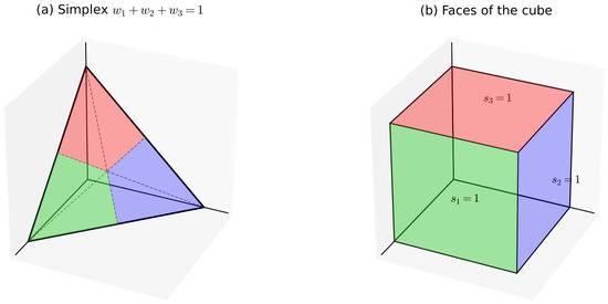
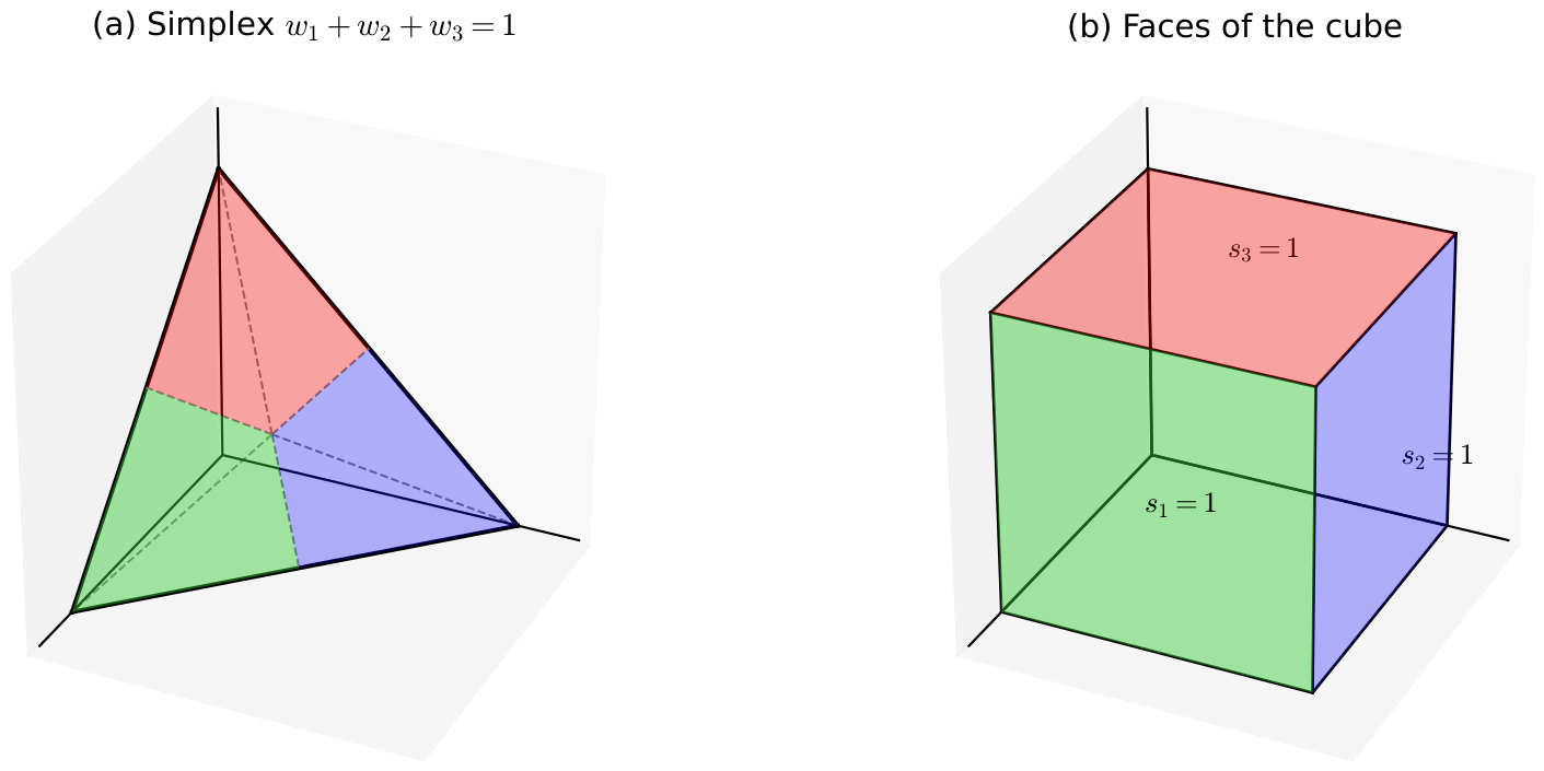
Given $\mathit{w}={(w_1,w_2,\dots ,w_n)}^{\top }$ with $0<w_i⩽1$, $1⩽i⩽n$, and ${\sum }_{i=1}^n{w}_i=1$, consider $\mathit{s}={(s_1,s_2,\dots ,s_n)}^{\top }$ with $s_i=w_i/M$, and $M={max}_{1⩽i⩽n}{w}_i$. Note that $0<s_i⩽1$, $1⩽i⩽n$, and there exists at least one index ı with s_ı $= 1$. The priority vector $\mathit{w}$ is in the probability simplex, which means that $\mathit{s}$ is in some face of the unit hypercube in the n-dimensional Euclidean space. For example, consider $n=3$. The probability simplex is a triangle. There are three regions with different colors. They are mapped to three squares $G_i$ as faces of the unit cube by the Belton–Gear normalization, where

$$G_i=\{{(s_1,s_2,s_3)}^{\top }:s_i=1,s_j\in (0,1],j\ne i,1⩽j⩽3\},1⩽i⩽3.$$

Figure 1 presents the probability simplex and the unit cube with colored faces given $n=3$. The three colored regions are separated by segments of the three bisectors (dashed lines). Within each region, one coordinate dominates the other two coordinates. The Belton–Gear normalization maps the three regions into three faces of the unit cube, with the images bearing the same colors as the pre-images.

Figure 1. The probability simplex and the faces of the unit cube given $n=3$.

3.2. The Addition of a New Option

When the new option $x_{n+1}$ is added, the updated version of ${\overline{\mathit{s}}}_n$ in (37) is

$${\overline{\mathit{s}}}_{n+1}=\sum _{\ell =1}^m{\lambda }_{\ell }{\left(s_{\ell }(x_1,\mathcal{K}),s_{\ell }(x_2,\mathcal{K}),\dots ,s_{\ell }(x_n,\mathcal{K}),s_{\ell }(x_{n+1},\mathcal{K})\right)}^{\top }.$$

(38)

The first n entries of ${\overline{\mathit{s}}}_{n+1}$ in (38) yield a subvector

$${\mathit{t}}_n^{*}=\sum _{\ell =1}^m{\lambda }_{\ell }{\left(s_{\ell }(x_1,\mathcal{K}),s_{\ell }(x_2,\mathcal{K}),\dots ,s_{\ell }(x_n,\mathcal{K})\right)}^{\top }.$$

(39)

The following presents the relationship between the entries of ${\mathit{t}}_n^{*}$ in (39) and those of ${\overline{\mathit{s}}}_n$ in (37).

Theorem 3.

Given ℓ with $1⩽\ell ⩽m$, the Belton–Gear scores $s_{\ell }(x_i,\mathcal{Q})$ and their updated versions $s_{\ell }(x_i,\mathcal{K})$ satisfy

$$s_{\ell }(x_i,\mathcal{K})={\nu }_{\ell }·s_{\ell }(x_i,\mathcal{Q}),1⩽i⩽n,$$

(40)

where

$${\nu }_{\ell }={\displaystyle \frac{M_{\ell }\left(\mathcal{Q}\right)}{max(M_{\ell }\left(\mathcal{Q}\right),{\theta }_{\ell })}}\in (0,1].$$

(41)

The relationships in (40) and (41) hold due to the cardinal consistency of the pertinent pairwise comparison matrices and the Belton–Gear normalization shown in Figure 1. The proof of Theorem 3 in Appendix A presents a detailed introduction to the proportionality arising from cardinal consistency.

Note that (8) and (40) are similar in structure. While (8) allows Yan and Mao [26] to reformulate ${\mathit{u}}_n^{*}$ in (10) as the version in (11), (40) allows us to reformulate ${\mathit{t}}_n^{*}$ in (39) as

$${\mathit{t}}_n^{*}=\sum _{\ell =1}^m{\lambda }_{\ell }{\nu }_{\ell }{\mathit{s}}_{\ell }.$$

(42)

Let $C_2={\sum }_{\ell =1}^m{\lambda }_{\ell }{\nu }_{\ell }$ and $a_{\ell }={\lambda }_{\ell }{\nu }_{\ell }/C_2$, $1⩽\ell ⩽m$. Note that

$$a_{\ell }\in (0,1),1⩽\ell ⩽m,\sum _{\ell =1}^m{a}_{\ell }=1.$$

(43)

The re-scaled version of ${\mathit{t}}_n^{*}$ in (42) is ${\mathit{t}}_n={\mathit{t}}_n^{*}/C_2$, i.e.,

$${\mathit{t}}_n=\sum _{\ell =1}^m{a}_{\ell }{\mathit{s}}_{\ell }.$$

(44)

Because of (3) and (43), both ${\overline{\mathit{s}}}_n$ in (37) and ${\mathit{t}}_n$ in (44) are convex combinations of the score vectors ${\mathit{s}}_{\ell }$ in (36). Similarly, the rank reversal problem in the Belton–Gear framework can be studied by focusing on (37) and (44).

3.3. The Geometric Approach

Because rank reversal is evaluated pairwise, it is natural to focus on a pair of options, for instance, options $x_j$ and $x_k$. This motivates focusing on the two options $x_j$ and $x_k$ [26]. To this end, we also consider the set ${\mathcal{E}}_{j,k}$ of m subvectors, where

$${\mathcal{E}}_{j,k}={\left\{{(s_{\ell }(x_j,\mathcal{Q}),s_{\ell }(x_k,\mathcal{Q}))}^{\top }\right\}}_{\ell =1}^m.$$

(45)

Note that ${\mathcal{E}}_{j,k}$ is a subset of the square A, where

$$A={(0,1]}^2=\{\mathit{y}\in {\mathbb{R}}^2:\mathit{y}={(y_1,y_2)}^{\top },0<y_1⩽1,0<y_2⩽1\}.$$

(46)

The diagonal line D from ${(0,0)}^{\top }$ to ${(1,1)}^{\top }$ divides A into two triangles $\overline{D}$ and $\underline{D}$, where

$$\begin{array}{cc}\hfill D& =\{\mathit{y}\in {\mathbb{R}}^2:\mathit{y}={(y_1,y_2)}^{\top },0<y_1⩽1,0<y_2⩽1,y_1=y_2\},\hfill \end{array}$$

(47)

$$\begin{array}{cc}\hfill \overline{D}& =\{\mathit{y}\in {\mathbb{R}}^2:\mathit{y}={(y_1,y_2)}^{\top },0<y_1⩽1,0<y_2⩽1,y_1<y_2\},\hfill \end{array}$$

(48)

$$\begin{array}{cc}\hfill \underline{D}& =\{\mathit{y}\in {\mathbb{R}}^2:\mathit{y}={(y_1,y_2)}^{\top },0<y_1⩽1,0<y_2⩽1,y_1>y_2\}.\hfill \end{array}$$

(49)

Note that D in (47) is also a bisector of A in (46).

There are also four scenarios, i.e.,

$$\left\{\begin{array}{cc}{\mathcal{E}}_{j,k}\subset \overline{D}\cup D,{\mathcal{E}}_{j,k}\cap \overline{D}\ne \varnothing \hfill & (\mathrm{scenario}1),\hfill \\ {\mathcal{E}}_{j,k}\subset \underline{D}\cup D,{\mathcal{E}}_{j,k}\cap \underline{D}\ne \varnothing \hfill & (\mathrm{scenario}2),\hfill \\ {\mathcal{E}}_{j,k}\subset D\hfill & (\mathrm{scenario}3),\hfill \\ {\mathcal{E}}_{j,k}\cap \overline{D}\ne \varnothing ,{\mathcal{E}}_{j,k}\cap \underline{D}\ne \varnothing \hfill & (\mathrm{scenario}4).\hfill \end{array}\right.$$

(50)

Clearly, ${\overline{\mathit{s}}}_n$ in (37) admits a subvector ${\mathit{p}}_{j,k}$, and ${\mathit{t}}_n^{*}$ in (39) admits a subvector ${\mathit{q}}_{j,k}^{*}$ with a scaled version ${\mathit{q}}_{j,k}={\mathit{q}}_{j,k}^{*}/C_2$ as a subvector of ${\mathit{t}}_n$ in (44), where

$$\begin{array}{cc}\hfill {\mathit{p}}_{j,k}& =\sum _{\ell =1}^m{\lambda }_{\ell }{(s_{\ell }(x_j,\mathcal{Q}),s_{\ell }(x_k,\mathcal{Q}))}^{\top },\hfill \end{array}$$

(51)

$$\begin{array}{cc}\hfill {\mathit{q}}_{j,k}^{*}& =\sum _{\ell =1}^m{\lambda }_{\ell }{(s_{\ell }(x_j,\mathcal{K}),s_{\ell }(x_k,\mathcal{K}))}^{\top }.\hfill \end{array}$$

(52)

Both ${\mathit{p}}_{j,k}$ and ${\mathit{q}}_{j,k}$ are convex combinations of vectors in the set ${\mathcal{E}}_{j,k}$ in (45).

Theorem 4.

The four scenarios in (50) can also be described as follows.

$$\left\{\begin{array}{cc}conv\left({\mathcal{E}}_{j,k}\right)\subset \overline{D}\cup D,conv\left({\mathcal{E}}_{j,k}\right)\cap \overline{D}\ne \varnothing \hfill & \left(scenario1\right),\hfill \\ conv\left({\mathcal{E}}_{j,k}\right)\subset \underline{D}\cup D,conv\left({\mathcal{E}}_{j,k}\right)\cap \underline{D}\ne \varnothing \hfill & \left(scenario2\right),\hfill \\ conv\left({\mathcal{E}}_{j,k}\right)\subset D\hfill & \left(scenario3\right),\hfill \\ conv\left({\mathcal{E}}_{j,k}\right)\cap \overline{D}\ne \varnothing ,conv\left({\mathcal{E}}_{j,k}\right)\cap \underline{D}\ne \varnothing \hfill & \left(scenario4\right).\hfill \end{array}\right.$$

(53)

Let ${\mathit{S}}_n$ denote the score matrix, where

$${\mathit{S}}_n=\left({\mathit{s}}_1,{\mathit{s}}_2,\dots ,{\mathit{s}}_m\right).$$

(54)

Define

$$\begin{array}{cc}\hfill {\rho }_{j,k}\left({\mathit{S}}_n\right)& =I\left({\mathcal{E}}_{j,k}\subset \overline{D}\cup D\right)+I\left({\mathcal{E}}_{j,k}\subset \underline{D}\cup D\right)-I\left({\mathcal{E}}_{j,k}\subset D\right),\hfill \end{array}$$

(55)

$$\begin{array}{cc}\hfill \rho \left({\mathit{S}}_n\right)& =\prod _{1⩽j<k⩽n}{\rho }_{j,k}\left({\mathit{S}}_n\right).\hfill \end{array}$$

(56)

Theorem 5.

Given $1⩽j<k⩽n$, the rank reversal problem between the two options $x_j$ and $x_k$ is infeasible if and only if ${\rho }_{j,k}\left({\mathit{S}}_n\right)=1$, and the rank reversal problem among these n options is infeasible if and only if $\rho \left({\mathit{S}}_n\right)=1$.

When the score matrix ${\mathit{S}}_n$ in (54) replaces the priority matrix ${\mathit{W}}_n$ in (23), Theorem 2 becomes Theorem 5.

We are also interested in the relationship between (19) and (50).

Theorem 6.

Given an option pair $(j,k)$, it holds that

$$\begin{array}{cc}\hfill {\mathcal{F}}_{j,k}\subset \overline{B}& ⟺{\mathcal{E}}_{j,k}\subset \overline{D},\hfill \end{array}$$

(57)

$$\begin{array}{cc}\hfill {\mathcal{F}}_{j,k}\subset \underline{B}& ⟺{\mathcal{E}}_{j,k}\subset \underline{D},\hfill \end{array}$$

(58)

$$\begin{array}{cc}\hfill {\mathcal{F}}_{j,k}\subset B& ⟺{\mathcal{E}}_{j,k}\subset D.\hfill \end{array}$$

(59)

Note that Theorem 6 is derived from the proportional relationships in (34), which serves as the foundation of the equivalence between the Saaty framework and the Belton–Gear framework in terms of the infeasibility of rank reversal.

3.4. The Algebraic Approach

We can also introduce the feasibility matrix based on scores in (34). Let

$$\begin{array}{cc}\hfill {\omega }_{\ell }(j,k)& =sign\left(s_{\ell }(x_j,\mathcal{Q})-s_{\ell }(x_k,\mathcal{Q})\right),\hfill \\ \hfill \mathit{\omega }(j,k)& ={\left({\omega }_1(j,k),{\omega }_2(j,k),\dots ,{\omega }_m(j,k)\right)}^{\top }.\hfill \end{array}$$

The feasibility matrix $\mathsf{\Omega }$ consists of the $\mathit{\omega }(j,k)$ as columns in lexicographic order, where

$$\mathsf{\Omega }=\left(\mathit{\omega }(1,2),\mathit{\omega }(1,3),\dots ,\mathit{\omega }(1,n),\mathit{\omega }(2,3),\dots ,\mathit{\omega }(2,n),\dots ,\mathit{\omega }(n-1,n)\right).$$

(60)

Theorem 7.

The feasibility matrix in (28) and that in (60) are identical, i.e.,

$$\mathsf{\Sigma }=\mathsf{\Omega }.$$

(61)

We can also introduce quantities like $\delta (j,k)$ in (30) and $\chi (j,k)$ in (32) based on $\mathsf{\Omega }$, which do not require additional symbols because they are identical to their counterparts based on $\mathsf{\Sigma }$.

Theorem 7 shows that the Belton–Gear normalization does not alter the feasibility structure of rank reversal and therefore cannot eliminate the phenomenon at the feasibility level.

The infeasibility of rank reversal is a property of the score matrix ${\mathit{S}}_n$ or, equivalently, the priority matrix ${\mathit{W}}_n$, as we can see from both Theorems 5 and 7 and Theorem 1 in Yan and Mao [26].

Finally, the realization of rank reversal not only demands feasibility but also depends on the added new option.

4. Illustration

4.1. The Belton–Gear Example

The example was proposed in Belton and Gear [10]. Yan and Mao [26] have studied the Belton–Gear example. There are three options ($n=3$) and three criteria ($m=3$), with ${\lambda }_{\ell }=1/3$, $\ell =1$, 2, 3. The matrix ${\mathit{W}}_n$ in (23) is given in the following,

$${\mathit{W}}_3=\left(\begin{array}{ccc}1/11& 9/11& 8/18\\ 9/11& 1/11& 9/18\\ 1/11& 1/11& 1/18\end{array}\right).$$

As $M_1\left(\mathcal{Q}\right)=9/11$, $M_2\left(\mathcal{Q}\right)=9/11$, and $M_3\left(\mathcal{Q}\right)=9/18$, ${\mathit{S}}_n$ in (54) is given by

$${\mathit{S}}_3=\left(\begin{array}{ccc}1/9& 1& 8/9\\ 1& 1/9& 1\\ 1/9& 1/9& 1/9\end{array}\right).$$

The feasibility matrix is

$$\mathsf{\Sigma }=\mathsf{\Omega }=\begin{array}{cc}\text{option pair}& (1,2)(1,3)(2,3)\\ \begin{array}{c}\text{criterion 1}\\ \text{criterion 2}\\ \text{criterion 3}\end{array}& \left[\begin{array}{ccc}-1& 0& 1\\ 1& 1& 0\\ -1& 1& 1\end{array}\right]\end{array}.$$

This means that rank reversal is feasible as

$$\chi (1,2)=0,\chi (1,3)=1,\chi (2,3)=1⟹\chi \left(\mathsf{\Sigma }\right)=\chi (1,2)\chi (1,3)\chi (2,3)=0.$$

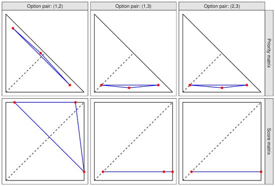
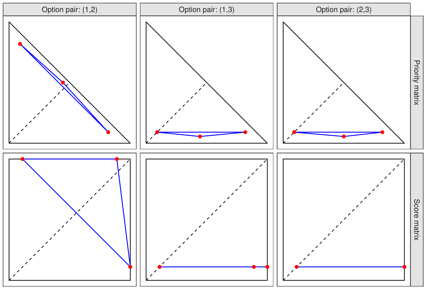
Figure 2 presents the convex hulls arising from the priority matrix ${\mathit{W}}_3$ and those from the score matrix ${\mathit{S}}_3$. Both convex hulls ${\mathcal{F}}_{1,2}$ and ${\mathcal{E}}_{1,2}$ cross the bisectors. From the score matrix, we obtain

$${\mathcal{E}}_{1,3}=\left\{\left({\displaystyle \genfrac{}{}{0pt}{}{1/9}{1/9}}\right),\left({\displaystyle \genfrac{}{}{0pt}{}{1}{1/9}}\right),\left({\displaystyle \genfrac{}{}{0pt}{}{8/9}{1/9}}\right)\right\}.$$

As the three points share the same $y_2$-coordinates, they are on the same line, and the convex hull becomes a line segment shown in Figure 2. In addition,

$${\mathcal{E}}_{2,3}=\left\{\left({\displaystyle \genfrac{}{}{0pt}{}{1}{1/9}}\right),\left({\displaystyle \genfrac{}{}{0pt}{}{1/9}{1/9}}\right),\left({\displaystyle \genfrac{}{}{0pt}{}{1}{1/9}}\right)\right\}.$$

There are only two distinct points in ${\mathcal{E}}_{2,3}$ that are on the same line, which means that the convex hull becomes a line segment, shown in Figure 2.

Figure 2. Belton–Gear example: convex hulls for option pairs $(1,2)$, $(1,3)$ and $(2,3)$, top row from the priority matrix and bottom row from the score matrix.

After a new option is added, the matrix of priorities becomes

$${\mathit{W}}_4=\left(\begin{array}{ccc}1/20& 9/12& 8/27\\ 9/20& 1/12& 9/27\\ 1/20& 1/12& 1/27\\ 9/20& 1/12& 9/27\end{array}\right).$$

The matrix of scores becomes

$${\mathit{S}}_4=\left(\begin{array}{ccc}1/9& 1& 8/9\\ 1& 1/9& 1\\ 1/9& 1/9& 1/9\\ 1& 1/9& 1\end{array}\right).$$

Given ${\lambda }_{\ell }=1/3$ for $\ell =1$, 2, 3, by some simple algebra, we obtain

$$\begin{array}{c}{w}_1(x_4,\mathcal{K})={\displaystyle \frac{9}{20}},w_2(x_4,\mathcal{K})={\displaystyle \frac{1}{12}},w_3(x_4,\mathcal{K})={\displaystyle \frac{9}{27}}={\displaystyle \frac{1}{3}},\\ {\gamma }_1={\displaystyle \frac{11}{20}},{\gamma }_2={\displaystyle \frac{11}{12}},{\gamma }_3={\displaystyle \frac{2}{3}},\\ {\theta }_1={\displaystyle \frac{9}{11}}=M_1\left(\mathcal{Q}\right),{\theta }_2={\displaystyle \frac{1}{11}}<{\displaystyle \frac{9}{11}}=M_2\left(\mathcal{Q}\right),{\theta }_3={\displaystyle \frac{1}{2}}=M_3\left(\mathcal{Q}\right),\\ {\nu }_1=1,{\nu }_2=1,{\nu }_3=1,\\ C_1={\displaystyle \frac{1}{3}}\left({\displaystyle \frac{11}{20}}+{\displaystyle \frac{11}{12}}+{\displaystyle \frac{2}{3}}\right)={\displaystyle \frac{32}{45}},\\ C_2={\displaystyle \frac{1}{3}}(1+1+1)=1.\end{array}$$

Because ${\nu }_1={\nu }_2={\nu }_3=1$, ${\mathit{t}}_n^{*}$ in (39) and ${\mathit{t}}_n$ in (44) are identical.

The aggregate vectors are given by

$$\begin{array}{c}{\overline{\mathit{w}}}_3={\displaystyle \frac{1}{594}}\left(\begin{array}{c}268\\ 279\\ 47\end{array}\right),{\overline{\mathit{w}}}_4={\displaystyle \frac{1}{1620}}\left(\begin{array}{c}592\\ 468\\ 92\\ 468\end{array}\right),{\overline{\mathit{s}}}_3={\displaystyle \frac{1}{27}}\left(\begin{array}{c}18\\ 19\\ 3\end{array}\right),{\overline{\mathit{s}}}_4={\displaystyle \frac{1}{27}}\left(\begin{array}{c}18\\ 19\\ 3\\ 19\end{array}\right).\end{array}$$

The four vectors used for comparison are given in Table 1. Under the condition that rank reversal is feasible, rank reversal is realized in the Saaty framework, while rank reversal is not realized in the Belton–Gear framework, as one can see from the following facts.

$${\mathit{\varphi }}_{12}\in \overline{B},{\mathit{\psi }}_{12}\in \underline{B},{\mathit{p}}_{12}={\mathit{q}}_{12}\in \overline{D}.$$

Table 1. Belton–Gear example: comparison vectors for three option pairs under the Saaty framework and the Belton–Gear framework.

	Saaty		Belton–Gear
$(\mathit{j},\mathit{k})$	$\mathit{\varphi }$	$\mathit{\psi }$	$\mathit{p}$	$\mathit{q}$
$(1,2)$	${\displaystyle \frac{1}{594}}\left(\begin{array}{c}268\\ 279\end{array}\right)$	${\displaystyle \frac{1}{288}}\left(\begin{array}{c}148\\ 117\end{array}\right)$	${\displaystyle \frac{1}{27}}\left(\begin{array}{c}18\\ 19\end{array}\right)$	${\displaystyle \frac{1}{27}}\left(\begin{array}{c}18\\ 19\end{array}\right)$
$(1,3)$	${\displaystyle \frac{1}{594}}\left(\begin{array}{c}268\\ 47\end{array}\right)$	${\displaystyle \frac{1}{288}}\left(\begin{array}{c}148\\ 23\end{array}\right)$	${\displaystyle \frac{1}{27}}\left(\begin{array}{c}18\\ 3\end{array}\right)$	${\displaystyle \frac{1}{27}}\left(\begin{array}{c}18\\ 3\end{array}\right)$
$(2,3)$	${\displaystyle \frac{1}{594}}\left(\begin{array}{c}279\\ 47\end{array}\right)$	${\displaystyle \frac{1}{288}}\left(\begin{array}{c}117\\ 23\end{array}\right)$	${\displaystyle \frac{1}{27}}\left(\begin{array}{c}19\\ 3\end{array}\right)$	${\displaystyle \frac{1}{27}}\left(\begin{array}{c}19\\ 3\end{array}\right)$

Finally, the ranks from the aggregate vectors are presented as follows,

$$\left\{\begin{array}{cc}{x}_2\succ x_1\succ x_3\hfill & \left({\overline{\mathit{w}}}_3\right),\hfill \\ x_1\succ x_2\sim x_4\succ x_3\hfill & \left({\overline{\mathit{w}}}_4\right),\hfill \\ x_2\succ x_1\succ x_3\hfill & \left({\overline{\mathit{s}}}_3\right),\hfill \\ x_4\sim x_2\succ x_1\succ x_3\hfill & \left({\overline{\mathit{s}}}_4\right),\hfill \end{array}\right.$$

where $a\succ b$ means that a is preferable to b, and $a\sim b$ means that a and b are indifferent.

4.2. The Saaty–Vargas Example

There are two options ($n=2$) under three criteria ($m=3$) with ${\lambda }_{\ell }=1/3$, $\ell =1$, 2, 3 [11]. Three pairwise comparison matrices proposed in Saaty and Vargas [11] are

$$\left(\begin{array}{cc}1& 1/2\\ 2& 1\end{array}\right),\left(\begin{array}{cc}1& 7/6\\ 6/7& 1\end{array}\right),\left(\begin{array}{cc}1& 3\\ 1/3& 1\end{array}\right).$$

The matrix of priorities in (23) is

$${\mathit{W}}_2=\left(\begin{array}{ccc}1/3& 7/13& 3/4\\ 2/3& 6/13& 1/4\end{array}\right).$$

Note that

$$M_1\left(\mathcal{Q}\right)={\displaystyle \frac{2}{3}},M_2\left(\mathcal{Q}\right)={\displaystyle \frac{7}{13}},M_3\left(\mathcal{Q}\right)={\displaystyle \frac{3}{4}}.$$

The matrix of scores in (54) is

$${\mathit{S}}_2=\left(\begin{array}{ccc}1/2& 1& 1\\ 1& 6/7& 1/3\end{array}\right).$$

The feasibility matrix has only one column, i.e.,

$$\mathsf{\Sigma }=\mathsf{\Omega }={(-1,1,1)}^{\top }.$$

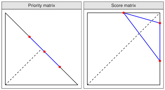
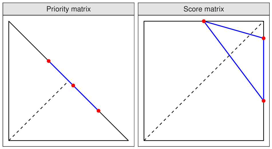
Because $\chi (1,2)=0$ and $\chi \left(\mathsf{\Sigma }\right)=0$, rank reversal is feasible. Figure 3 presents the convex hull from the priority matrix and that from the score matrix. Both convex hulls cross the bisectors. As $n=2$, ${\mathcal{F}}_{12}$ is on the line $y_1+y_2=1$, and its convex hull is a line segment, shown in Figure 3.

Figure 3. Saaty–Vargas example: convex hulls for the option pair $(1,2)$, left from the priority matrix and right from the score matrix.

When a new option is added, the updated pairwise comparison matrices are

$$\left(\begin{array}{ccc}1& 1/2& 1/2\\ 2& 1& 1\\ 2& 1& 1\end{array}\right),\left(\begin{array}{ccc}1& 7/6& 1\\ 6/7& 1& 6/7\\ 1& 7/6& 1\end{array}\right),\left(\begin{array}{ccc}1& 3& 1/2\\ 1/3& 1& 1/6\\ 2& 6& 1\end{array}\right),$$

as proposed in Saaty and Vargas [11]. The updated priority matrix is

$${\mathit{W}}_3=\left(\begin{array}{ccc}1/5& 7/20& 3/10\\ 2/5& 6/20& 1/10\\ 2/5& 7/20& 6/10\end{array}\right),$$

and the updated score matrix is

$${\mathit{S}}_3=\left(\begin{array}{ccc}1/2& 1& 3/6\\ 1& 6/7& 1/6\\ 1& 1& 1\end{array}\right).$$

Simple algebra yields

$$\begin{array}{c}{w}_1(x_3,\mathcal{K})={\displaystyle \frac{2}{5}},w_2(x_3,\mathcal{K})={\displaystyle \frac{7}{20}},w_3(x_3,\mathcal{K})={\displaystyle \frac{3}{5}},\\ {\gamma }_1={\displaystyle \frac{3}{5}},{\gamma }_2={\displaystyle \frac{13}{20}},{\gamma }_3={\displaystyle \frac{2}{5}},\\ {\theta }_1={\displaystyle \frac{2}{3}}=M_1\left(\mathcal{Q}\right),{\theta }_2={\displaystyle \frac{7}{13}}=M_2\left(\mathcal{Q}\right),{\theta }_3={\displaystyle \frac{3}{2}}>M_3\left(\mathcal{Q}\right)={\displaystyle \frac{3}{4}},\\ {\nu }_1=1,{\nu }_2=1,{\nu }_3={\displaystyle \frac{1}{2}},\\ C_1={\displaystyle \frac{1}{3}}\left({\displaystyle \frac{3}{5}}+{\displaystyle \frac{13}{20}}+{\displaystyle \frac{2}{5}}\right)={\displaystyle \frac{11}{20}},\\ C_2={\displaystyle \frac{1}{3}}\left(1+1+{\displaystyle \frac{1}{2}}\right)={\displaystyle \frac{5}{6}}.\end{array}$$

The aggregated vectors are

$$\begin{array}{c}\hfill {\overline{\mathit{w}}}_2={\displaystyle \frac{1}{468}}\left(\begin{array}{c}253\\ 215\end{array}\right),{\overline{\mathit{s}}}_2={\displaystyle \frac{1}{126}}\left(\begin{array}{c}105\\ 92\end{array}\right),{\overline{\mathit{w}}}_3={\displaystyle \frac{1}{60}}\left(\begin{array}{c}17\\ 16\\ 27\end{array}\right),{\overline{\mathit{s}}}_3={\displaystyle \frac{1}{126}}\left(\begin{array}{c}84\\ 85\\ 126\end{array}\right).\end{array}$$

There is only one option pair with indices $(1,2)$, and the four vectors used for comparison are given as follows,

$$\begin{array}{cc}\hfill {\mathit{\varphi }}_{12}={\displaystyle \frac{1}{468}}\left({\displaystyle \genfrac{}{}{0pt}{}{253}{215}}\right)& \mathrm{versus}{\mathit{\psi }}_{12}={\displaystyle \frac{1}{33}}\left({\displaystyle \genfrac{}{}{0pt}{}{17}{16}}\right),\hfill \\ \hfill {\mathit{p}}_{12}={\displaystyle \frac{1}{126}}\left({\displaystyle \genfrac{}{}{0pt}{}{105}{92}}\right)& \mathrm{versus}{\mathit{q}}_{12}={\displaystyle \frac{1}{105}}\left({\displaystyle \genfrac{}{}{0pt}{}{84}{85}}\right).\hfill \end{array}$$

Under the condition that rank reversal is feasible, rank reversal is not realized in the Saaty framework, while it is realized in the Belton–Gear framework, because

$${\mathit{\varphi }}_{12}\in \underline{B},{\mathit{\psi }}_{12}\in \underline{B},{\mathit{p}}_{12}\in \underline{D},{\mathit{q}}_{12}\in \overline{D}.$$

Finally, the ranks from the aggregate vectors are presented as follows:

$$\left\{\begin{array}{cc}{x}_1\succ x_2\hfill & \left({\overline{\mathit{w}}}_2\right),\hfill \\ x_3\succ x_1\succ x_2\hfill & \left({\overline{\mathit{w}}}_3\right),\hfill \\ x_1\succ x_2\hfill & \left({\overline{\mathit{s}}}_2\right),\hfill \\ x_3\succ x_2\succ x_1\hfill & \left({\overline{\mathit{s}}}_3\right).\hfill \end{array}\right.$$

4.3. The Yan–Mao Examples

Yan and Mao [26] propose four synthetic examples labeled by A, B, C and D, each with three options and three criteria ($n=3,m=3$). Their priority matrices are presented as follows:

$$\begin{array}{c}\hfill {\mathit{W}}_A={\displaystyle \frac{1}{12}}\left(\begin{array}{ccc}1& 1& 9\\ 1& 9& 1\\ 9& 2& 2\end{array}\right),{\mathit{W}}_B={\displaystyle \frac{1}{12}}\left(\begin{array}{ccc}1& 1& 4\\ 2& 9& 3\\ 9& 2& 5\end{array}\right),\\ \hfill {\mathit{W}}_C={\displaystyle \frac{1}{12}}\left(\begin{array}{ccc}1& 1& 3\\ 2& 9& 4\\ 9& 2& 5\end{array}\right),{\mathit{W}}_D={\displaystyle \frac{1}{12}}\left(\begin{array}{ccc}1& 1& 3\\ 2& 3& 4\\ 9& 8& 5\end{array}\right).\end{array}$$

Table 2 presents the score matrices ${\mathit{S}}_n$ and feasibility matrices $\mathsf{\Omega }$.

Table 2. Yan–Mao examples: score matrices and feasibility matrices.

Example	Score Matrix ${\mathit{S}}_3$	Feasibility Matrix $\mathsf{\Omega }$
A	${\displaystyle \left(\begin{array}{ccc}1/9& 1/9& 1\\ 1/9& 1& 1/9\\ 1& 2/9& 2/9\end{array}\right)}$	${\displaystyle \left(\begin{array}{ccc}0& -1& -1\\ -1& -1& 1\\ 1& 1& -1\end{array}\right)}$
B	${\displaystyle \left(\begin{array}{ccc}1/9& 1/9& 4/5\\ 2/9& 1& 3/5\\ 1& 2/9& 1\end{array}\right)}$	${\displaystyle \left(\begin{array}{ccc}-1& -1& -1\\ -1& -1& 1\\ 1& -1& -1\end{array}\right)}$
C	${\displaystyle \left(\begin{array}{ccc}1/9& 1/9& 3/5\\ 2/9& 1& 4/5\\ 1& 2/9& 1\end{array}\right)}$	${\displaystyle \left(\begin{array}{ccc}-1& -1& -1\\ -1& -1& 1\\ -1& -1& -1\end{array}\right)}$
D	${\displaystyle \left(\begin{array}{ccc}1/9& 1/8& 3/5\\ 2/9& 3/8& 4/5\\ 1& 1& 1\end{array}\right)}$	${\displaystyle \left(\begin{array}{ccc}-1& -1& -1\\ -1& -1& -1\\ -1& -1& -1\end{array}\right)}$

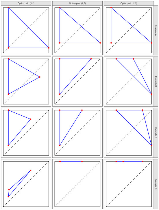
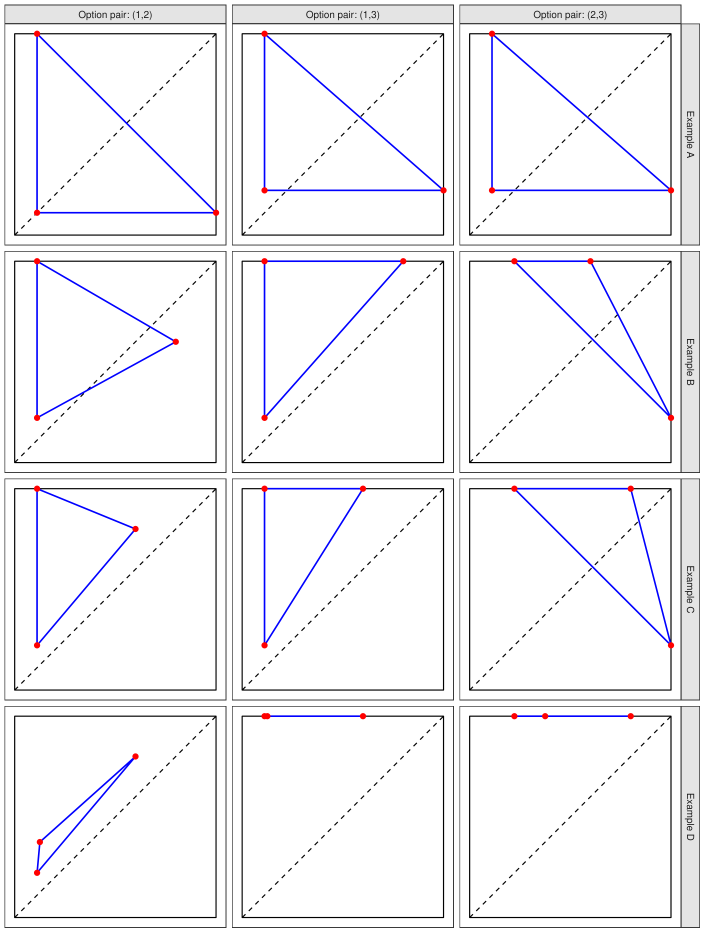
Figure 4 presents the convex hulls of ${\mathcal{E}}_{j,k}$. We consider comparing Figure 3 in Yan and Mao [26] against Figure 4.

Figure 4. Yan–Mao examples: convex hulls for three option pairs from score matrices, left column for pair $(1,2)$, middle for $(1,3)$, and right for $(2,3)$.

• Example A: The convex hull $conv\left({\mathcal{E}}_{j,k}\right)$ crosses the bisector D, while $conv\left({\mathcal{F}}_{j,k}\right)$ crosses the bisector B for $(j,k)=(1,2)$, $(1,3)$ and $(2,3)$.
• Example B: The convex hulls $conv\left({\mathcal{E}}_{1,2}\right)$ and $conv\left({\mathcal{E}}_{2,3}\right)$ cross D, while $conv\left({\mathcal{F}}_{1,2}\right)$ and $conv\left({\mathcal{F}}_{2,3}\right)$ cross B; $conv\left({\mathcal{E}}_{1,3}\right)$ is contained in $\overline{D}$, while $conv\left({\mathcal{F}}_{1,3}\right)$ is contained in $\overline{B}$.
• Example C: The convex hull $conv\left({\mathcal{E}}_{2,3}\right)$ crosses D, while $conv\left({\mathcal{F}}_{2,3}\right)$ crosses B; both $conv\left({\mathcal{E}}_{1,2}\right)$ and $conv\left({\mathcal{E}}_{1,3}\right)$ are contained in $\overline{D}$, while both $conv\left({\mathcal{F}}_{1,2}\right)$ and $conv\left({\mathcal{F}}_{1,3}\right)$ are contained in $\overline{B}$.
• Example D: The convex hull $conv\left({\mathcal{E}}_{j,k}\right)$ is contained in $\overline{D}$, while $conv\left({\mathcal{F}}_{j,k}\right)$ is contained in $\overline{B}$ for $(j,k)=(1,2)$, $(1,3)$ and $(2,3)$. Both $conv\left({\mathcal{E}}_{1,3}\right)$ and $conv\left({\mathcal{E}}_{2,3}\right)$ are line segments because, from Table 2,

  $$\begin{array}{c}\hfill {\mathcal{E}}_{1,3}=\left\{\left({\displaystyle \genfrac{}{}{0pt}{}{1/9}{1}}\right),\left({\displaystyle \genfrac{}{}{0pt}{}{1/8}{1}}\right),\left({\displaystyle \genfrac{}{}{0pt}{}{3/5}{1}}\right)\right\}\mathrm{and}{\mathcal{E}}_{2,3}=\left\{\left({\displaystyle \genfrac{}{}{0pt}{}{2/9}{1}}\right),\left({\displaystyle \genfrac{}{}{0pt}{}{3/8}{1}}\right),\left({\displaystyle \genfrac{}{}{0pt}{}{4/5}{1}}\right)\right\}.\end{array}$$

  It is clear that these results are expected from Theorems 1, 4 and 6.

To compare the geometric approach and the algebraic approach, we present the indicator, where the convex hull ${\mathcal{E}}_{j,k}$ crosses the bisector D or not, and the infeasibility indicator $\chi (j,k)$ in Table 3, where ✓ and $\chi (j,k)=0$ represent the crossing and feasibility, while × and $\chi (j,k)=1$ represent not-crossing and infeasibility. The two approaches are clearly equivalent.

Table 3. Yan–Mao examples: crossing the bisector and algebraic infeasibility indicators.

	Crossing the Bisector			Infeasibility Indicator $\mathit{\chi }$
$(\mathit{j},\mathit{k})$	(1, 2)	(1, 3)	(2, 3)	(1, 2)	(1, 3)	(2, 3)
A	✓	✓	✓	0	0	0
B	✓	×	✓	0	1	0
C	×	×	✓	1	1	0
D	×	×	×	1	1	1

4.4. Example: Realizations Given Different Added Options

We now present an example showing that, once rank reversal is feasible, its realization depends on the introduced option. Starting from the same original pairwise comparison matrices, four different added options lead to four possible outcomes: no rank reversal in either the Saaty framework or the Belton–Gear framework, rank reversal only in the Saaty framework, rank reversal only in the Belton–Gear framework, and rank reversal in both frameworks.

There are three options ($n=3$) under two criteria ($m=2$), with ${\lambda }_1=3/5$ and ${\lambda }_2=2/5$. The two pairwise comparison matrices are

$$A_1=\left(\begin{array}{ccc}1& 2& 6\\ 1/2& 1& 3\\ 1/6& 1/3& 1\end{array}\right),A_2=\left(\begin{array}{ccc}1& 1/2& 3\\ 2& 1& 6\\ 1/3& 1/6& 1\end{array}\right).$$

Both matrices are cardinally consistent. Their priority vectors are

$${\mathit{w}}_1={\displaystyle \frac{1}{10}}\left(\begin{array}{c}6\\ 3\\ 1\end{array}\right),{\mathit{w}}_2={\displaystyle \frac{1}{10}}\left(\begin{array}{c}3\\ 6\\ 1\end{array}\right).$$

(62)

The aggregate priority vector is

$${\overline{\mathit{w}}}_3={\displaystyle \frac{3}{5}}{\mathit{w}}_1+{\displaystyle \frac{2}{5}}{\mathit{w}}_2={\displaystyle \frac{1}{50}}\left(\begin{array}{c}24\\ 21\\ 5\end{array}\right).$$

(63)

Under the Belton–Gear normalization, since

$$M_1\left(\mathcal{Q}\right)=M_2\left(\mathcal{Q}\right)={\displaystyle \frac{3}{5}},$$

the score vectors are

$${\mathit{s}}_1={\displaystyle \frac{1}{6}}\left(\begin{array}{c}6\\ 3\\ 1\end{array}\right),{\mathit{s}}_2={\displaystyle \frac{1}{6}}\left(\begin{array}{c}3\\ 6\\ 1\end{array}\right).$$

(64)

The aggregate score vector is

$${\overline{\mathit{s}}}_3={\displaystyle \frac{3}{5}}{\mathit{s}}_1+{\displaystyle \frac{2}{5}}{\mathit{s}}_2={\displaystyle \frac{1}{30}}\left(\begin{array}{c}24\\ 21\\ 5\end{array}\right).$$

(65)

For the option pair $(x_1,x_2)$, we have

$$\begin{array}{cc}\hfill {\sigma }_1(1,2)& =sign(w_1(x_1,\mathcal{Q})-w_1(x_2,\mathcal{Q}))=sign\left({\displaystyle \frac{6}{10}}-{\displaystyle \frac{3}{10}}\right)=sign{\displaystyle \frac{3}{10}}=1,\hfill \\ \hfill {\sigma }_2(1,2)& =sign(w_2(x_1,\mathcal{Q})-w_2(x_2,\mathcal{Q}))=sign\left({\displaystyle \frac{3}{10}}-{\displaystyle \frac{6}{10}}\right)=sign{\displaystyle \frac{-3}{10}}=-1.\hfill \end{array}$$

The two criteria induce opposite signs, which means that rank reversal is feasible.

We next introduce four different added options, each represented by two updated consistent pairwise comparison matrices.

Case 1: Two updated consistent pairwise comparison matrices are

$$A_1^{\left(1\right)}=\left(\begin{array}{cccc}1& 2& 6& 12/5\\ 1/2& 1& 3& 6/5\\ 1/6& 1/3& 1& 2/5\\ 5/12& 5/6& 5/2& 1\end{array}\right),A_2^{\left(1\right)}=\left(\begin{array}{cccc}1& 1/2& 3& 6/5\\ 2& 1& 6& 12/5\\ 1/3& 1/6& 1& 2/5\\ 5/6& 5/12& 5/2& 1\end{array}\right).$$

The priority vectors are

$${\mathit{w}}_1^{\left(1\right)}={\displaystyle \frac{1}{25}}\left(\begin{array}{c}12\\ 6\\ 2\\ 5\end{array}\right),{\mathit{w}}_2^{\left(1\right)}={\displaystyle \frac{1}{25}}\left(\begin{array}{c}6\\ 12\\ 2\\ 5\end{array}\right).$$

(66)

The aggregate vector is

$${\overline{\mathit{w}}}_4^{\left(1\right)}={\displaystyle \frac{3}{5}}{\mathit{w}}_1^{\left(1\right)}+{\displaystyle \frac{2}{5}}{\mathit{w}}_2^{\left(1\right)}={\displaystyle \frac{1}{125}}\left(\begin{array}{c}48\\ 42\\ 10\\ 25\end{array}\right).$$

(67)

Since $M_1\left({\mathcal{K}}^{\left(1\right)}\right)=12/25$, and $M_2\left({\mathcal{K}}^{\left(1\right)}\right)=12/25$, the score vectors are

$${\mathit{s}}_1^{\left(1\right)}={\displaystyle \frac{1}{12}}\left(\begin{array}{c}12\\ 6\\ 2\\ 5\end{array}\right),{\mathit{s}}_2^{\left(1\right)}={\displaystyle \frac{1}{12}}\left(\begin{array}{c}6\\ 12\\ 2\\ 5\end{array}\right).$$

(68)

The aggregate score vector is

$${\overline{\mathit{s}}}_4^{\left(1\right)}={\displaystyle \frac{3}{5}}{\mathit{s}}_1^{\left(1\right)}+{\displaystyle \frac{2}{5}}{\mathit{s}}_2^{\left(1\right)}={\displaystyle \frac{1}{60}}\left(\begin{array}{c}48\\ 42\\ 10\\ 25\end{array}\right).$$

(69)

Case 2: Two updated consistent pairwise comparison matrices are

$$A_1^{\left(2\right)}=\left(\begin{array}{cccc}1& 2& 6& 11/15\\ 1/2& 1& 3& 11/30\\ 1/6& 1/3& 1& 11/90\\ 15/11& 30/11& 90/11& 1\end{array}\right),A_2^{\left(2\right)}=\left(\begin{array}{cccc}1& 1/2& 3& 27/10\\ 2& 1& 6& 27/5\\ 1/3& 1/6& 1& 9/10\\ 10/27& 5/27& 10/9& 1\end{array}\right).$$

The priority vectors are

$${\mathit{w}}_1^{\left(2\right)}={\displaystyle \frac{1}{200}}\left(\begin{array}{c}66\\ 33\\ 11\\ 90\end{array}\right),{\mathit{w}}_2^{\left(2\right)}={\displaystyle \frac{1}{100}}\left(\begin{array}{c}27\\ 54\\ 9\\ 10\end{array}\right).$$

(70)

The aggregate priority vector is

$${\overline{\mathit{w}}}_4^{\left(2\right)}={\displaystyle \frac{3}{5}}{\mathit{w}}_1^{\left(2\right)}+{\displaystyle \frac{2}{5}}{\mathit{w}}_2^{\left(2\right)}={\displaystyle \frac{1}{1000}}\left(\begin{array}{c}306\\ 315\\ 69\\ 310\end{array}\right).$$

(71)

Since $M_1\left({\mathcal{K}}^{\left(2\right)}\right)=90/200$, and $M_2\left({\mathcal{K}}^{\left(2\right)}\right)=54/100$, the score vectors are

$${\mathit{s}}_1^{\left(2\right)}={\displaystyle \frac{1}{90}}\left(\begin{array}{c}66\\ 33\\ 11\\ 90\end{array}\right),{\mathit{s}}_2^{\left(2\right)}={\displaystyle \frac{1}{54}}\left(\begin{array}{c}27\\ 54\\ 9\\ 10\end{array}\right).$$

(72)

The aggregate score vector is

$${\overline{\mathit{s}}}_4^{\left(2\right)}={\displaystyle \frac{3}{5}}{\mathit{s}}_1^{\left(2\right)}+{\displaystyle \frac{2}{5}}{\mathit{s}}_2^{\left(2\right)}={\displaystyle \frac{1}{1350}}\left(\begin{array}{c}864\\ 837\\ 189\\ 910\end{array}\right).$$

(73)

Case 3: Two updated consistent pairwise comparison matrices are

$$A_1^{\left(3\right)}=\left(\begin{array}{cccc}1& 2& 6& 9/35\\ 1/2& 1& 3& 9/70\\ 1/6& 1/3& 1& 3/70\\ 35/9& 70/9& 70/3& 1\end{array}\right),A_2^{\left(3\right)}=\left(\begin{array}{cccc}1& 1/2& 3& 1/5\\ 2& 1& 6& 2/5\\ 1/3& 1/6& 1& 1/15\\ 5& 5/2& 15& 1\end{array}\right).$$

The corresponding priority vectors are

$${\mathit{w}}_1^{\left(3\right)}={\displaystyle \frac{1}{100}}\left(\begin{array}{c}18\\ 9\\ 3\\ 70\end{array}\right),{\mathit{w}}_2^{\left(3\right)}={\displaystyle \frac{1}{25}}\left(\begin{array}{c}3\\ 6\\ 1\\ 15\end{array}\right).$$

(74)

The aggregate priority vector is

$${\overline{\mathit{w}}}_4^{\left(3\right)}={\displaystyle \frac{3}{5}}{\mathit{w}}_1^{\left(3\right)}+{\displaystyle \frac{2}{5}}{\mathit{w}}_2^{\left(3\right)}={\displaystyle \frac{1}{500}}\left(\begin{array}{c}78\\ 75\\ 17\\ 330\end{array}\right).$$

(75)

Since $M_1\left({\mathcal{K}}^{\left(3\right)}\right)=70/100$, and $M_2\left({\mathcal{K}}^{\left(3\right)}\right)=15/25$, the score vectors are

$${\mathit{s}}_1^{\left(3\right)}={\displaystyle \frac{1}{70}}\left(\begin{array}{c}18\\ 9\\ 3\\ 70\end{array}\right),{\mathit{s}}_2^{\left(3\right)}={\displaystyle \frac{1}{15}}\left(\begin{array}{c}3\\ 6\\ 1\\ 15\end{array}\right).$$

(76)

The aggregate score vector is

$${\overline{\mathit{s}}}_4^{\left(3\right)}={\displaystyle \frac{3}{5}}{\mathit{s}}_1^{\left(3\right)}+{\displaystyle \frac{2}{5}}{\mathit{s}}_2^{\left(3\right)}={\displaystyle \frac{1}{1050}}\left(\begin{array}{c}246\\ 249\\ 55\\ 1050\end{array}\right).$$

(77)

Case 4: Two updated consistent pairwise comparison matrices are

$$A_1^{\left(4\right)}=\left(\begin{array}{cccc}1& 2& 6& 9/35\\ 1/2& 1& 3& 9/70\\ 1/6& 1/3& 1& 3/70\\ 35/9& 70/9& 70/3& 1\end{array}\right),A_2^{\left(4\right)}=\left(\begin{array}{cccc}1& 1/2& 3& 6/5\\ 2& 1& 6& 12/5\\ 1/3& 1/6& 1& 2/5\\ 5/6& 5/12& 5/2& 1\end{array}\right).$$

The priority vectors are

$${\mathit{w}}_1^{\left(4\right)}={\displaystyle \frac{1}{100}}\left(\begin{array}{c}18\\ 9\\ 3\\ 70\end{array}\right),{\mathit{w}}_2^{\left(4\right)}={\displaystyle \frac{1}{25}}\left(\begin{array}{c}6\\ 12\\ 2\\ 5\end{array}\right).$$

(78)

The aggregate priority vector is

$${\overline{\mathit{w}}}_4^{\left(4\right)}={\displaystyle \frac{3}{5}}{\mathit{w}}_1^{\left(4\right)}+{\displaystyle \frac{2}{5}}{\mathit{w}}_2^{\left(4\right)}={\displaystyle \frac{1}{500}}\left(\begin{array}{c}102\\ 123\\ 25\\ 250\end{array}\right).$$

(79)

Since $M_1\left({\mathcal{K}}^{\left(4\right)}\right)=70/100$, and $M_2\left({\mathcal{K}}^{\left(4\right)}\right)=12/25$, the score vectors are

$${\mathit{s}}_1^{\left(4\right)}={\displaystyle \frac{1}{70}}\left(\begin{array}{c}18\\ 9\\ 3\\ 70\end{array}\right),{\mathit{s}}_2^{\left(4\right)}={\displaystyle \frac{1}{12}}\left(\begin{array}{c}6\\ 12\\ 2\\ 5\end{array}\right).$$

(80)

The aggregate score vector is

$${\overline{\mathit{s}}}_4^{\left(4\right)}={\displaystyle \frac{3}{5}}{\mathit{s}}_1^{\left(4\right)}+{\displaystyle \frac{2}{5}}{\mathit{s}}_2^{\left(4\right)}={\displaystyle \frac{1}{1050}}\left(\begin{array}{c}372\\ 501\\ 97\\ 805\end{array}\right).$$

(81)

The aggregate priority vectors in (63), (67), (71), (75) and (79) in the Saaty framework generate the rankings respectively, as follows:

$$\begin{array}{cc}\hfill \mathrm{Before}\mathrm{addition}:& x_1\succ x_2\succ x_3,\hfill \end{array}$$

(82)

$$\begin{array}{cc}\hfill \mathrm{After}\mathrm{addition}:& \left\{\begin{array}{cc}{x}_1\succ x_2\succ x_4\succ x_3\hfill & \left(\mathrm{Case}1\right)\hfill \\ x_2\succ x_4\succ x_1\succ x_3\hfill & \left(\mathrm{Case}2\right)\hfill \\ x_4\succ x_1\succ x_2\succ x_3\hfill & \left(\mathrm{Case}3\right)\hfill \\ x_4\succ x_2\succ x_1\succ x_3\hfill & \left(\mathrm{Case}4\right)\hfill \end{array}\right..\hfill \end{array}$$

(83)

The aggregate score vectors in (65), (69), (73), (77) and (81) in the Belton–Gear framework generate the rankings respectively, as follows:

$$\begin{array}{cc}\hfill \mathrm{Before}\mathrm{addition}:& x_1\succ x_2\succ x_3,\hfill \end{array}$$

(84)

$$\begin{array}{cc}\hfill \mathrm{After}\mathrm{addition}:& \left\{\begin{array}{cc}{x}_1\succ x_2\succ x_4\succ x_3\hfill & \left(\mathrm{Case}1\right)\hfill \\ x_4\succ x_1\succ x_2\succ x_3\hfill & \left(\mathrm{Case}2\right)\hfill \\ x_4\succ x_2\succ x_1\succ x_3\hfill & \left(\mathrm{Case}3\right)\hfill \\ x_4\succ x_2\succ x_1\succ x_3\hfill & \left(\mathrm{Case}4\right)\hfill \end{array}\right..\hfill \end{array}$$

(85)

Finally, the four cases are summarized as follows:

$$\left\{\begin{array}{c}\mathrm{Case}1:\mathrm{no}\mathrm{rank}\mathrm{reversal}\mathrm{in}\mathrm{either}\mathrm{framework},\hfill \\ \mathrm{Case}2:\mathrm{rank}\mathrm{reversal}\mathrm{only}\mathrm{in}\mathrm{the}\mathrm{Saaty}\mathrm{framework},\hfill \\ \mathrm{Case}3:\mathrm{rank}\mathrm{reversal}\mathrm{only}\mathrm{in}\mathrm{the}\mathrm{Belton–Gear}\mathrm{framework},\hfill \\ \mathrm{Case}4:\mathrm{rank}\mathrm{reversal}\mathrm{in}\mathrm{both}\mathrm{frameworks},\hfill \end{array}\right.$$

(86)

which can be obtained by comparing (83) against (82) and comparing (85) against (84).

This example shows that feasibility is a property of the original priority matrix or score matrix, but realization depends on the introduced option. Even when the original matrices are fixed, and rank reversal is feasible, different added options may lead to different outcomes in the Saaty framework and the Belton–Gear framework.

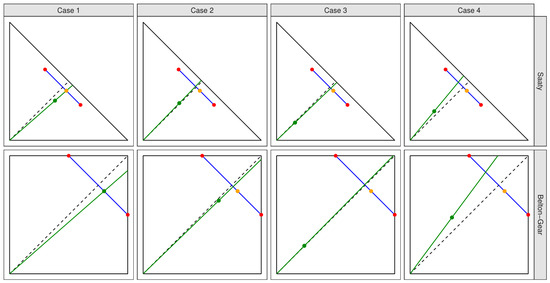
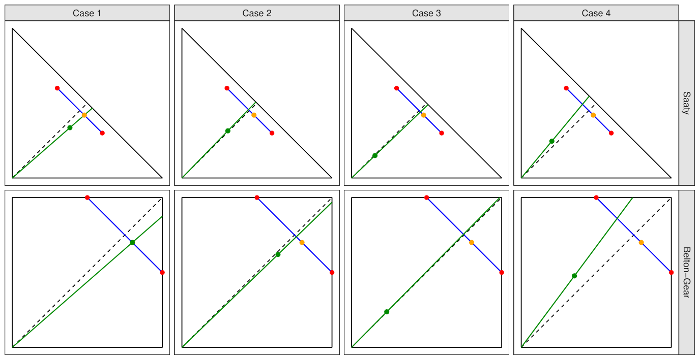
Given the option pair $(1,2)$, Figure 5 presents the subvectors extracted from the priority vectors, i.e., ${(w_{\ell }(x_1,\mathcal{Q}),w_{\ell }(x_2,\mathcal{Q}))}^{\top }$ (red points) from (62), $\ell =1$ and 2, and ${(w_{\ell }^{\left(h\right)}(x_1,{\mathcal{K}}^{\left(h\right)}),w_{\ell }^{\left(h\right)}(x_2,{\mathcal{K}}^{\left(h\right)}))}^{\top }$ (red points) from (66), (70), (74) and (78), $\ell =1$ and 2, $h=1$, 2, 3 and 4; those from the aggregate priority vectors, i.e., ${\mathit{\varphi }}_{12}$ (orange points) from (63), and ${\mathit{\psi }}_{12}^{*}$ (green points) from (67), (71), (75) and (79); those from the score vectors, i.e., ${(s_{\ell }(x_1,\mathcal{Q}),s_{\ell }(x_2,\mathcal{Q}))}^{\top }$ (red points) from (64), $\ell =1$, 2, and ${(s_{\ell }^{\left(h\right)}(x_1,{\mathcal{K}}^{\left(h\right)}),s_{\ell }^{\left(h\right)}(x_2,{\mathcal{K}}^{\left(h\right)}))}^{\top }$ (red points) from (68), (72), (76) and (80), $\ell =1$ and 2, $h=1$, 2, 3 and 4; and those from the aggregate score vectors, i.e., ${\mathit{p}}_{12}$ from (65) (orange points), and ${\mathit{q}}_{1,2}^{*}$ (green points) from (69), (73), (77) and (81). In each plot, the convex hull of the two red points is a line segment (solid blue line segment), and the solid green ray from the origin through one green point is also shown, together with the bisector (dashed black line). The solid green rays can be compared against the bisectors. If a green ray and the orange point are in the same side of the bisector, then rank reversal does not occur, and otherwise, rank reversal occurs.

Figure 5. Example: realizations given different added options.

For Case 1, the green point and the orange point are on the same green ray because ${\mathit{\varphi }}_{12}=(5/4)·{\mathit{\psi }}_{12}^{*}$ in the Saaty framework, and the green point and the orange point coincide because ${\mathit{p}}_{12}={\mathit{q}}_{12}^{*}$ in the Belton–Gear framework, where

$$\begin{array}{cccccc}\hfill & \hfill & \hfill {\mathit{\varphi }}_{12}& ={\displaystyle \frac{1}{50}}\left({\displaystyle \genfrac{}{}{0pt}{}{24}{21}}\right)={\displaystyle \frac{1}{4}}·{\displaystyle \frac{6}{25}}\left({\displaystyle \genfrac{}{}{0pt}{}{8}{7}}\right),\hfill & \hfill {\mathit{p}}_{12}& ={\displaystyle \frac{1}{30}}\left({\displaystyle \genfrac{}{}{0pt}{}{24}{21}}\right)={\displaystyle \frac{1}{10}}\left({\displaystyle \genfrac{}{}{0pt}{}{8}{7}}\right),\hfill \\ \hfill \mathrm{Case}1:& \hfill & \hfill {\mathit{\psi }}_{12}^{*}& ={\displaystyle \frac{1}{125}}\left({\displaystyle \genfrac{}{}{0pt}{}{48}{42}}\right)={\displaystyle \frac{1}{5}}·{\displaystyle \frac{6}{25}}\left({\displaystyle \genfrac{}{}{0pt}{}{8}{7}}\right),\hfill & \hfill {\mathit{q}}_{12}^{*}& ={\displaystyle \frac{1}{60}}\left({\displaystyle \genfrac{}{}{0pt}{}{48}{42}}\right)={\displaystyle \frac{1}{10}}\left({\displaystyle \genfrac{}{}{0pt}{}{8}{7}}\right).\hfill \end{array}$$

For Case 2 and Case 3, the solid green rays and the black dashed bisectors are close to each other because the two coordinates of a green point (${\mathit{\psi }}_{12}^{*}$ in the Saaty framework or ${\mathit{q}}_{12}^{*}$ in the Belton–Gear framework) are slightly different from each other, where

$$\begin{array}{cccccc}\hfill \mathrm{Case}2:& \hfill & \hfill {\mathit{\psi }}_{12}^{*}& ={\displaystyle \frac{1}{1000}}\left({\displaystyle \genfrac{}{}{0pt}{}{306}{315}}\right)={\displaystyle \frac{9}{1000}}\left({\displaystyle \genfrac{}{}{0pt}{}{34}{35}}\right),\hfill & \hfill {\mathit{q}}_{12}^{*}& ={\displaystyle \frac{1}{1350}}\left({\displaystyle \genfrac{}{}{0pt}{}{864}{837}}\right)={\displaystyle \frac{1}{50}}\left({\displaystyle \genfrac{}{}{0pt}{}{32}{31}}\right),\hfill \\ \hfill \mathrm{Case}3:& \hfill & \hfill {\mathit{\psi }}_{12}^{*}& ={\displaystyle \frac{1}{500}}\left({\displaystyle \genfrac{}{}{0pt}{}{78}{75}}\right)={\displaystyle \frac{3}{500}}\left({\displaystyle \genfrac{}{}{0pt}{}{26}{25}}\right),\hfill & \hfill {\mathit{q}}_{12}^{*}& ={\displaystyle \frac{1}{1050}}\left({\displaystyle \genfrac{}{}{0pt}{}{246}{249}}\right)={\displaystyle \frac{1}{350}}\left({\displaystyle \genfrac{}{}{0pt}{}{82}{83}}\right).\hfill \end{array}$$

For Case 4, the solid green rays and the black dashed bisectors are well separated because

$$\begin{array}{cccccc}\hfill \mathrm{Case}4:& \hfill & \hfill {\mathit{\psi }}_{12}^{*}& ={\displaystyle \frac{1}{500}}\left({\displaystyle \genfrac{}{}{0pt}{}{102}{123}}\right),\phantom{={\displaystyle \frac{1}{500}}\left({\displaystyle \genfrac{}{}{0pt}{}{102}{123}}\right)}\hfill & \hfill {\mathit{q}}_{12}^{*}& ={\displaystyle \frac{1}{1050}}\left({\displaystyle \genfrac{}{}{0pt}{}{372}{501}}\right)={\displaystyle \frac{1}{350}}\left({\displaystyle \genfrac{}{}{0pt}{}{124}{167}}\right).\hfill \end{array}$$

The scaled vectors ${\mathit{\psi }}_{12}={\mathit{\psi }}_{12}^{*}/C_1$ and ${\mathit{q}}_{12}={\mathit{q}}_{12}^{*}/C_2$ are in the convex hulls of the two red points and are shown as the intersections of the solid blue lines and solid green rays, where

$$\begin{array}{cccccc}\hfill \mathrm{Case}1:& \hfill & \hfill C_1& ={\displaystyle \frac{4}{5}},\hfill & \hfill C_2& =1,\hfill \\ \hfill \mathrm{Case}2:& \hfill & \hfill C_1& ={\displaystyle \frac{69}{100}},\hfill & \hfill C_2& ={\displaystyle \frac{21}{25}},\hfill \\ \hfill \mathrm{Case}3:& \hfill & \hfill C_1& ={\displaystyle \frac{17}{50}},\hfill & \hfill C_2& ={\displaystyle \frac{11}{35}},\hfill \\ \hfill \mathrm{Case}4:& \hfill & \hfill C_1& ={\displaystyle \frac{1}{2}},\hfill & \hfill C_2& ={\displaystyle \frac{97}{175}}.\hfill \end{array}$$

Nevertheless, the same conclusions as those in (86) can be obtained from Figure 5.

4.5. Example: Cardinally Inconsistent Pairwise Comparison Matrices

The infeasibility condition established in Section 2 and Section 3 is derived under the assumption of cardinal consistency. We now present an example showing that our results cannot be directly extended to cardinally inconsistent pairwise comparison matrices when priorities are derived by the principal eigenvector method.

Consider three options ($n=3$) under two criteria ($m=2$), with ${\lambda }_1={\lambda }_2=1/2$. The two pairwise comparison matrices are

$$A_1=\left(\begin{array}{ccc}1& 9& 8\\ 1/9& 1& 3\\ 1/8& 1/3& 1\end{array}\right),A_2=\left(\begin{array}{ccc}1& 4& 6\\ 1/4& 1& 3\\ 1/6& 1/3& 1\end{array}\right).$$

Both matrices are cardinally inconsistent as $a_{12|\ell }{a}_{23|\ell }\ne a_{13|\ell }$, $\ell =1$, 2, i.e.,

$$9\times 3=27\ne 8\mathrm{in}{A}_1,4\times 3=12\ne 6\mathrm{in}{A}_2.$$

Using the principal eigenvector method, we obtain the priority vectors

$${\mathit{w}}_1=\left(\begin{array}{c}0.8000\\ 0.1333\\ 0.0667\end{array}\right),{\mathit{w}}_2=\left(\begin{array}{c}0.6910\\ 0.2176\\ 0.0914\end{array}\right).$$

(87)

The aggregate priority vector is

$${\overline{\mathit{w}}}_3={\displaystyle \frac{1}{2}}{\mathit{w}}_1+{\displaystyle \frac{1}{2}}{\mathit{w}}_2\approx \left(\begin{array}{c}0.7455\\ 0.1755\\ 0.0791\end{array}\right).$$

Next, we check the algebraic infeasibility condition. The feasibility matrix is

$$\Sigma =\begin{array}{cc}\text{option pair}& (1,2)(1,3)(2,3)\\ \begin{array}{c}\text{criterion 1}\\ \text{criterion 2}\end{array}& \left[\begin{array}{ccc}1& 1& 1\\ 1& 1& 1\end{array}\right]\end{array}.$$

This means that

$$\begin{array}{c}\chi (1,2)=1,\chi (1,3)=1,\chi (2,3)=1,\\ \chi \left(\mathsf{\Sigma }\right)=\chi (1,2)\chi (1,3)\chi (2,3)=1.\end{array}$$

According to the algebraic infeasibility condition developed for the consistent case, rank reversal is infeasible.

We add a new option $x_4$ by presenting two updated pairwise comparison matrices:

$$B_1=\left(\begin{array}{cccc}1& 9& 8& 1\\ 1/9& 1& 3& 3\\ 1/8& 1/3& 1& 9\\ 1& 1/3& 1/9& 1\end{array}\right),B_2=\left(\begin{array}{cccc}1& 4& 6& 1\\ 1/4& 1& 3& 1\\ 1/6& 1/3& 1& 7\\ 1& 1& 1/7& 1\end{array}\right).$$

Again, using the principal eigenvector method, we obtain

$${\mathit{w}}_1^{\prime }=\left(\begin{array}{c}0.5394\\ 0.1648\\ 0.1888\\ 0.1070\end{array}\right),{\mathit{w}}_2^{\prime }=\left(\begin{array}{c}0.4529\\ 0.1872\\ 0.2231\\ 0.1368\end{array}\right).$$

(88)

The aggregate priority vector becomes

$${\overline{\mathit{w}}}_4={\displaystyle \frac{1}{2}}{\mathit{w}}_1^{\prime }+{\displaystyle \frac{1}{2}}{\mathit{w}}_2^{\prime }\approx \left(\begin{array}{c}0.4962\\ 0.1760\\ 0.2060\\ 0.1219\end{array}\right).$$

Consider the Belton–Gear normalization. From ${\mathit{w}}_1$ and ${\mathit{w}}_2$ in (87), we obtain

$${\mathit{s}}_1={\displaystyle \frac{1}{0.8000}}\left(\begin{array}{c}0.8000\\ 0.1333\\ 0.0667\end{array}\right)\approx \left(\begin{array}{c}1.0000\\ 0.1666\\ 0.0834\end{array}\right),{\mathit{s}}_2={\displaystyle \frac{1}{0.6910}}\left(\begin{array}{c}0.6910\\ 0.2176\\ 0.0914\end{array}\right)\approx \left(\begin{array}{c}1.0000\\ 0.3149\\ 0.1323\end{array}\right).$$

Hence, the aggregate score vector is

$${\overline{\mathit{s}}}_3={\displaystyle \frac{1}{2}}{\mathit{s}}_1+{\displaystyle \frac{1}{2}}{\mathit{s}}_2\approx \left(\begin{array}{c}1.0000\\ 0.2408\\ 0.1079\end{array}\right).$$

Applying the Belton–Gear normalization to ${\mathit{w}}_1^{\prime }$ and ${\mathit{w}}_2^{\prime }$ in (88) gives

$${\mathit{s}}_1^{\prime }={\displaystyle \frac{1}{0.5394}}\left(\begin{array}{c}0.5394\\ 0.1648\\ 0.1888\\ 0.1070\end{array}\right)\approx \left(\begin{array}{c}1.0000\\ 0.3055\\ 0.3500\\ 0.1984\end{array}\right),{\mathit{s}}_2^{\prime }={\displaystyle \frac{1}{0.4529}}\left(\begin{array}{c}0.4529\\ 0.1872\\ 0.2231\\ 0.1368\end{array}\right)\approx \left(\begin{array}{c}1.0000\\ 0.4133\\ 0.4926\\ 0.3021\end{array}\right).$$

Therefore, the updated aggregate score vector is

$${\overline{\mathit{s}}}_4={\displaystyle \frac{1}{2}}{\mathit{s}}_1^{\prime }+{\displaystyle \frac{1}{2}}{\mathit{s}}_2^{\prime }\approx \left(\begin{array}{c}1.0000\\ 0.3594\\ 0.4213\\ 0.2503\end{array}\right).$$

Finally, the rankings from the aggregate vectors are presented as follows:

$$\left\{\begin{array}{cc}{x}_1\succ x_2\succ x_3\hfill & \left({\overline{\mathit{w}}}_3\right),\hfill \\ x_1\succ x_3\succ x_2\succ x_4\hfill & \left({\overline{\mathit{w}}}_4\right),\hfill \\ x_1\succ x_2\succ x_3\hfill & \left({\overline{\mathit{s}}}_3\right),\hfill \\ x_1\succ x_3\succ x_2\succ x_4\hfill & \left({\overline{\mathit{s}}}_4\right).\hfill \end{array}\right.$$

(89)

Thus, from (89), under both the Saaty framework and the Belton–Gear framework, the relative order of $x_2$ and $x_3$ is reversed after the introduction of $x_4$. This example shows that, for cardinally inconsistent pairwise comparison matrices under the principal eigenvector method, the infeasibility condition derived for the cardinally consistent case no longer guarantees the impossibility of rank reversal.

The reason is that, in the cardinally inconsistent case, the addition of a new option does not in general preserve the proportional relationships in (8) and (40), which play a fundamental role in the analysis of Section 2 and Section 3. Note that

$$\begin{array}{cccccc}\hfill {\displaystyle \frac{w_1^{\prime }\left(x_1\right)}{w_1\left(x_1\right)}}& ={\displaystyle \frac{0.5394}{0.8000}}\approx 0.67,\hfill & \hfill {\displaystyle \frac{w_1^{\prime }\left(x_2\right)}{w_1\left(x_2\right)}}& ={\displaystyle \frac{0.1648}{0.1333}}\approx 1.24,\hfill & \hfill {\displaystyle \frac{w_1^{\prime }\left(x_3\right)}{w_1\left(x_3\right)}}& ={\displaystyle \frac{0.1888}{0.0667}}\approx 2.83,\hfill \\ \hfill {\displaystyle \frac{w_2^{\prime }\left(x_1\right)}{w_2\left(x_1\right)}}& ={\displaystyle \frac{0.4529}{0.6910}}\approx 0.66,\hfill & \hfill {\displaystyle \frac{w_2^{\prime }\left(x_2\right)}{w_2\left(x_2\right)}}& ={\displaystyle \frac{0.1872}{0.2176}}\approx 0.86,\hfill & \hfill {\displaystyle \frac{w_2^{\prime }\left(x_3\right)}{w_2\left(x_3\right)}}& ={\displaystyle \frac{0.2231}{0.0914}}\approx 2.44,\hfill \\ \hfill {\displaystyle \frac{s_1^{\prime }\left(x_1\right)}{s_1\left(x_1\right)}}& ={\displaystyle \frac{1}{1}}=1,\hfill & \hfill {\displaystyle \frac{s_1^{\prime }\left(x_2\right)}{s_1\left(x_2\right)}}& ={\displaystyle \frac{0.3055}{0.1666}}\approx 1.83,\hfill & \hfill {\displaystyle \frac{s_1^{\prime }\left(x_3\right)}{s_1\left(x_3\right)}}& ={\displaystyle \frac{0.3500}{0.0833}}\approx 4.20,\hfill \\ \hfill {\displaystyle \frac{s_2^{\prime }\left(x_1\right)}{s_2\left(x_1\right)}}& ={\displaystyle \frac{1}{1}}=1,\hfill & \hfill {\displaystyle \frac{s_2^{\prime }\left(x_2\right)}{s_2\left(x_2\right)}}& ={\displaystyle \frac{0.4133}{0.3149}}\approx 1.31,\hfill & \hfill {\displaystyle \frac{s_2^{\prime }\left(x_3\right)}{s_2\left(x_3\right)}}& ={\displaystyle \frac{0.4926}{0.1323}}\approx 3.72.\hfill \end{array}$$

The ratios in each row should be the same for the cardinally consistent case and actually vary for the cardinally inconsistent case. Hence, once cardinal consistency is abandoned, a different theoretical paradigm is required to study the infeasibility of rank reversal.

5. Conclusions

Although Belton and Gear [10] present the problem of rank reversal, their proposal of solving the issue of rank reversal does not achieve its claimed aim of eliminating rank reversals. Saaty and Vargas [11] use an example to show the failure of the proposal in Belton and Gear [10] without theoretical support. Our analysis indicates that when rank reversal is feasible, both the Saaty framework and the Belton–Gear framework have opportunities to realize rank reversal, i.e., they do not differ in terms of the feasibility of rank reversal. The conditions of the infeasibility of rank reversal are equivalent within both frameworks.

A key implication of our results is the distinction between the feasibility and the realization of rank reversal. While the feasibility is determined solely by the original matrix, the realization additionally depends on the introduced option. This distinction provides a unified explanation for the seemingly conflicting observations reported in the literature.

Beyond the Saaty and Belton–Gear frameworks, the proposed geometric and algebraic approaches offer a general analytical paradigm. In particular, the geometric perspective characterizes feasibility through convex structures and their interaction with bisectors, whereas the algebraic formulation enables efficient verification via sign patterns. These approaches may be naturally extended to other normalization or aggregation schemes.

References

- Saaty, T.L. A Scaling Method for Priorities in Hierarchical Structures. J. Math. Psychol. 1977, 15, 234–281. [Google Scholar] [CrossRef] [Scilit]
- Saaty, T.L. The Analytic Hierarchy Process; McGraw-Hill: New York, NY, USA, 1980. [Google Scholar]
- Saaty, T.L. How to Make a Decision: The Analytic Hierarchy Process. Eur. J. Oper. Res. 1990, 48, 9–26. [Google Scholar] [CrossRef] [Scilit]
- Brunelli, M. Introduction to the Analytic Hierarchy Process; Springer: Cham, Switzerland, 2015. [Google Scholar]
- Chaoui, G.; Yaagoubi, R.; Mastere, M. Integrating Geospatial Technologies and Multi-Criteria Decision Analysis for Sustainable and Resilient Urban Planning. Chall. Sustain. 2025, 13, 122–134. [Google Scholar] [CrossRef] [Scilit]
- Fedorka, P.; Buchuk, R.; Klymenko, M.; Saibert, F.; Petrushyn, A. The Use of Adaptive Artificial Intelligence Learning Models in Decision Support Systems for Smart Regions. J. Res. Innov. Technol. 2025, 4, 99–115. [Google Scholar]
- Terentieva, N.; Karpenko, V.; Yarova, N.; Shkvyria, N.; Pasko, M. Technological Innovation in Digital Brand Management: Leveraging Artificial Intelligence and Immersive Experiences. J. Res. Innov. Technol. 2025, 4, 201–223. [Google Scholar]
- Maleki, H.; Zahir, S. A Comprehensive Literature Review of the Rank Reversal Phenomenon in the Analytic Hierarchy Process. J. Multi-Criteria Decis. Anal. 2013, 20, 141–155. [Google Scholar] [CrossRef] [Scilit]
- Aires, R.F.F.; Ferreira, L. The rank reversal problem in multi-criteria decision making: A literature review. Pesqui. Oper. 2018, 38, 331–362. [Google Scholar] [CrossRef] [Scilit]
- Belton, V.; Gear, T. On a short-coming of Saaty’s method of analytic hierarchies. Omega 1983, 11, 228–230. [Google Scholar] [CrossRef] [Scilit]
- Saaty, T.L.; Vargas, L.G. The legitimacy of rank reversal. Omega 1984, 12, 513–516. [Google Scholar] [CrossRef] [Scilit]
- Belton, V.; Gear, T. The legitimacy of rank reversal—A comment. Omega 1985, 13, 143–144. [Google Scholar] [CrossRef] [Scilit]
- Schoner, B.; Wedley, W.C. Ambiguous criteria weights in AHP: Consequences and solutions. Decis. Sci. 1989, 20, 462–475. [Google Scholar] [CrossRef] [Scilit]
- Schoner, B.; Wedley, W.C.; Choo, E.U. A unified approach to AHP with linking pins. Eur. J. Oper. Res. 1993, 64, 384–392. [Google Scholar] [CrossRef] [Scilit]
- Lootsma, F.A. Scale sensitivity in the multiplicative AHP and SMART. J. Multi-Criteria Decis. Anal. 1993, 2, 87–110. [Google Scholar] [CrossRef] [Scilit]
- Barzilai, J.; Golany, B. AHP rank reversal, normalization and aggregation rules. INFOR Inf. Syst. Oper. Res. 1994, 32, 57–64. [Google Scholar] [CrossRef] [Scilit]
- Barzilai, J.; Lootsma, F.A. Power relations and group aggregation in the multiplicative AHP and SMART. J. Multi-Criteria Decis. Anal. 1997, 6, 155–165. [Google Scholar] [CrossRef]
- Lootsma, F.A.; Barzilai, J. Response to the comments by Larichev, Korhonen and Vargas. J. Multi-Criteria Decis. Anal. 1997, 6, 171–174. [Google Scholar] [CrossRef]
- Stam, A. Short note on “On the measurement of preferences in the analytic hierarchy process”. J. Multi-Criteria Decis. Anal. 1997, 6, 338–339. [Google Scholar] [CrossRef]
- Triantaphyllou, E. Two new cases of rank reversals when the AHP and some of its additive variants are used that do not occur with the multiplicative AHP. J. Multi-Criteria Decis. Anal. 2001, 10, 11–25. [Google Scholar] [CrossRef] [Scilit]
- Stam, A.; Silva, A.P.D. On multiplicative priority rating methods for the AHP. Eur. J. Oper. Res. 2003, 145, 92–108. [Google Scholar] [CrossRef] [Scilit]
- Tu, J.; Wu, Z. Analytic hierarchy process rank reversals: Causes and solutions. Ann. Oper. Res. 2025, 346, 1785–1809. [Google Scholar] [CrossRef] [Scilit]
- Krause, A.; Köppel, J. A multi-criteria approach for assessing the sustainability of small-scale cooking and sanitation technologies. Chall. Sustain. 2018, 6, 1–19. [Google Scholar] [CrossRef] [Scilit]
- Qiu, Y.; Bouraima, M.B.; Badi, I.; Stevic, Z.; Simic, V. A decision-making model for prioritizing low-carbon policies in climate change mitigation. Chall. Sustain. 2024, 12, 1–17. [Google Scholar] [CrossRef] [Scilit]
- Peng, D.; Liu, J.; Wu, S.; Yang, G. Discussion for the Belton–Gear normalization of analytic hierarchy process. IAENG Int. J. Appl. Math. 2025, 55, 553–564. [Google Scholar]
- Yan, J.; Mao, C. An infeasibility condition for rank reversal in the analytic hierarchy process. Axioms 2025, 14, 860. [Google Scholar] [CrossRef] [Scilit]
Disclaimer/Publisher’s Note: The statements, opinions and data contained in all publications are solely those of the individual author(s) and contributor(s) and not of MDPI and/or the editor(s). MDPI and/or the editor(s) disclaim responsibility for any injury to people or property resulting from any ideas, methods, instructions or products referred to in the content. |
© 2026 by the authors. Licensee MDPI, Basel, Switzerland. This article is an open access article distributed under the terms and conditions of the Creative Commons Attribution (CC BY) license.