Preservation of Mean-Square Lyapunov Exponents for Nonautonomous Stochastic Evolution Equations

Abstract

We study the long-time behavior of nonlinear stochastic evolution equations in a separable Hilbert space driven by a Q-Wiener process. The linear part of the equation is generated by a strongly continuous semigroup with an exponential dichotomy, which provides fixed rates of decay and growth. The nonlinear drift and diffusion terms are globally Lipschitz and become small as time tends to infinity. Our main result shows that under these conditions, the mean-square Lyapunov exponents of the nonlinear system coincide with those of the linear part. In other words, nonlinear stochastic perturbations that decay in time do not change the main growth or decay rates of solutions in the mean-square sense. This result provides simple and verifiable criteria ensuring that the long-time Lyapunov behavior of the nonlinear stochastic equation is fully determined by the linear semigroup, even in the presence of time-dependent stochastic perturbations.

1. Introduction

The asymptotic behavior of infinite-dimensional evolution equations under deterministic and stochastic perturbations is a fundamental problem with deep connections to stability theory, invariant manifold theory, and the qualitative analysis of stochastic partial differential equations. In many concrete models arising in physics, biology, and engineering, the linear part of the dynamics provides a natural splitting of the phase space into exponentially stable and unstable directions; this splitting is conveniently formalized by an exponential dichotomy of the linear semigroup. Understanding whether and how the asymptotic growth rates dictated by the linear part persist in the presence of (possibly multiplicative) stochastic forcing and nonlinear perturbations is the central question studied in this paper.

The asymptotic behavior of random dynamical systems, as $t\to \infty$, is important both in theory and in applications. A key tool in this area is the concept of exponential dichotomy for linear evolution equations, which is closely related to stability and long-time behavior of solutions. Classical results of Daleckii and Krein [1] describe conditions for exponential dichotomy of deterministic systems generated by $C_0$-semigroups and their spectral properties. Later, this idea became a standard tool in the study of perturbed linear and nonlinear systems, including stable and unstable manifolds and exponential stability.

For stochastic systems, the natural analogue is mean-square exponential dichotomy, which describes a splitting of the phase space into stable and unstable parts in the mean-square sense. In finite-dimensional systems, exponential dichotomy was studied in [2] using quadratic forms. The relation between dichotomy and bounded solutions of inhomogeneous systems was investigated in [3], and the persistence of dichotomy under small perturbations was studied in [4]. For infinite-dimensional stochastic systems, dichotomy was studied, for example, in [5,6].

The concept of exponential dichotomy is also closely related to Lyapunov exponents. In the linear case, dichotomy is expected when the Lyapunov exponents do not vanish. The basic theory of Lyapunov exponents for stochastic systems was developed in [7,8]. Later, Lyapunov exponents were used in many problems, including Hopf bifurcation with noise [9], lower bounds for Lyapunov exponents [10], ergodic theory [11], and synchronization of infinite-dimensional stochastic systems [12]. However, the preservation of Lyapunov exponents for infinite-dimensional stochastic systems under asymptotically vanishing perturbations has not been studied in the same form.

We consider stochastic evolution equations on a separable Hilbert space H of the form

$$\mathrm{d}y\left(t\right)=\left(Ay\left(t\right)+F(t,y(t\left)\right)\right)\mathrm{d}t+G(t,y\left(t\right))\mathrm{d}W\left(t\right),$$

(1)

where $A:D\left(A\right)\subset H\to H$ generates a strongly continuous semigroup ${\left\{e^{At}\right\}}_{t\ge 0}$ and W denotes a Q-Wiener process. The unperturbed linear semigroup is assumed to admit an exponential dichotomy on $[0,\infty )$: there is a bounded projection that splits $H=H^{-}\oplus H^{+}$ and a rate $\alpha >0$ so that solutions originating in the negative subspace $H^{-}$ decay exponentially at least at a rate $\alpha$, while those associated with the positive subspace $H^{+}$ grow at least at a rate $\alpha$. This linear dichotomy provides the reference exponents $\pm \alpha$ against which the perturbed dynamics will be measured.

The nonlinear terms are taken to satisfy two structural conditions. First, a global Lipschitz condition (assumption (H1)) ensures well posedness and permits mean-square estimates for solutions. Second, an asymptotic smallness condition (assumption (H2)) requires that the nonlinear drift and diffusion coefficients decay to zero, as $t\to \infty$, in a uniform, multiplicative manner. Intuitively, (H2) means that, for large times, the nonlinear stochastic perturbation becomes negligible in comparison with the linear dynamics; such a regime is natural in models with temporally vanishing forcing or coefficients and is crucial for comparing long-time growth rates with the linear reference.

Our main result (Theorem 1) states that, under (H1) and (H2), the asymptotic mean-square growth rates of nontrivial mild solutions coincide with the reference exponents provided by the linear dichotomy: any solution that remains bounded in mean-square decays with an upper mean-square Lyapunov exponent of at most $-\alpha$, while any solution whose mean-square norm diverges grows with a lower mean-square Lyapunov exponent of at least $+\alpha$. Equivalently, there is no intermediate mean-square growth rate: every nontrivial trajectory is either mean-square exponentially decaying or mean-square exponentially growing, and the corresponding mean-square Lyapunov exponent equals $\pm \alpha$. This preservation of mean-square Lyapunov exponents demonstrates a robust dichotomy of asymptotic dynamics for the full stochastic system.

From a conceptual viewpoint, the result highlights a form of spectral rigidity for mean-square growth rates: when nonlinear and stochastic perturbations decay in time, they cannot create new asymptotic mean-square growth rates distinct from those already present in the linear part. Practically, this gives a simple and computable criterion to classify long-time behavior of a large class of stochastic evolution equations by inspecting the linear generator and verifying the mild decay of perturbations.

The hypotheses adopted here strike a balance between generality and technical transparency. The global Lipschitz assumption could be relaxed in future work (for instance, to local Lipschitz with suitable dissipativity), and the asymptotic smallness condition might be weakened to integrability-type assumptions; both directions raise interesting technical challenges, especially in controlling stochastic convolutions without uniform Lipschitz estimates. We briefly discuss such extensions and open problems in the conclusion.

A heuristic way to understand the result is the following. The exponential dichotomy of the linear semigroup splits the phase space into directions that decay exponentially and directions that grow exponentially. When the nonlinear drift and diffusion terms become small, as $t\to \infty$, their influence on the dynamics over large time intervals is negligible compared with the exponential action of the linear semigroup.

If a trajectory had an intermediate growth rate, lying between the stable and unstable exponential rates, then the projections of the solution onto the stable and unstable subspaces would have to balance each other in a very precise way over arbitrarily long time intervals. However, the dichotomy estimates imply that the stable component is exponentially damped, while the unstable component is exponentially amplified. Since the perturbation terms become arbitrarily small for large times, they cannot maintain such a delicate balance. As a consequence, the solution must eventually align with either the stable or the unstable directions of the linear dynamics, which leads to exponential decay or exponential growth in the mean-square sense. The extension from finite-dimensional systems to stochastic evolution equations in Hilbert spaces is not purely notational. In many classical results on exponential dichotomy and the preservation of Lyapunov exponents for stochastic systems, the analysis relies on Lyapunov functions given by quadratic forms. Such approaches reduce stability questions to properties of the corresponding quadratic functional and its generator along the system.

In infinite-dimensional spaces, however, the existence of suitable quadratic Lyapunov functionals generally requires additional structural assumptions on the operator or on the underlying semigroup. Therefore, arguments based directly on quadratic forms are not always readily applicable in the abstract Hilbert space setting.

Another technical difference concerns compactness arguments that are often used implicitly in finite-dimensional proofs. In ${\mathbb{R}}^n$ the unit sphere is compact, which allows one to extract convergent subsequences and to perform certain maximization arguments. In an infinite-dimensional Hilbert space, the unit sphere is no longer compact, and such arguments cannot be used directly.

For this reason, the proof presented in this paper follows a different strategy. Instead of constructing Lyapunov functionals, we derive direct estimates for the second moment of the solution using the projections associated with the exponential dichotomy and elementary inequalities, such as the Cauchy–Schwarz inequality and Itô’s isometry. This leads to a simple comparison inequality that controls the present second moment of the solution by its past and future values.

From a methodological point of view, the proposed approach provides an alternative to the classical quadratic-form techniques and yields a relatively elementary proof of the preservation of mean-square Lyapunov exponents in the infinite-dimensional stochastic setting.

This paper is organized as follows. Immediately after this introduction, we present precise definitions, the standing hypotheses (H1)–(H2), the notion of a mild solution and mean-square Lyapunov exponents, and we state the main preservation theorem together with remarks on the interpretation of the driving noise (see Section 2). In Section 3, we give a detailed proof of Theorem 1. Section 4 contains two concrete examples that illustrate the applicability of the abstract result to simple stochastic evolution models. This manuscript concludes with a discussion in Section 5, outlining possible generalizations and further research directions.

• Notation. Throughout this paper $\parallel ·\parallel$ denotes the norm on H, $L\left(H\right)$ denotes the space of bounded linear operators on H, and ${\parallel ·\parallel }_{HS}$ is the Hilbert–Schmidt norm for operators where it appears. We work in the mean-square framework and use standard notions for stochastic integrals in Hilbert spaces.

2. Preliminaries and Problem Statement

2.1. Exponential Dichotomy of the Linear Part

We assume that the linear semigroup generated by A admits an exponential dichotomy on $[0,\infty )$ (see, e.g., [1,13]). More precisely, there exists a bounded projection $P_{-}\in L\left(H\right)$ inducing a decomposition

$$H=H^{-}\oplus H^{+},$$

where $H^{-}:=P_{-}H$, and $H^{+}:=(I-P_{-})H$, and constants $N\ge 1$, $\alpha >0$, such that

$$\parallel P_{-}{e}^{As}\parallel \le N{e}^{-\alpha s},\parallel P_{+}{e}^{-As}\parallel \le N{e}^{-\alpha s},s\ge 0,$$

(2)

where $P_{+}:=I-P_{-}$.

This dichotomy provides a reference splitting into exponentially stable and unstable directions for the unperturbed linear dynamics.

2.2. Assumptions on the Nonlinear Terms

Throughout this paper we impose the following standing hypotheses on the nonlinearities.

Hypothesis 1

(H1). Global Lipschitz continuity. There exists a constant $L>0$, such that, for all $t\ge 0$ and all $y_1,y_2\in H$,

$$\parallel F(t,y_1)-F(t,y_2)\parallel +\parallel G(t,y_1)-G(t,y_2){\parallel }_{HS} \le L\parallel y_1-y_2\parallel .$$

Hypothesis 2

(H2). Asymptotic smallness. There exists a scalar function $\epsilon :[0,\infty )\to [0,\infty )$ with $\epsilon \left(t\right)\to 0$, as $t\to \infty$, such that for all $t\ge 0$ and all $y\in H$

$$\parallel F(t,y)\parallel +{\parallel G(t,y)\parallel }_{HS}\le \epsilon \left(t\right)\parallel y\parallel .$$

Note that assumption (H2) implies $F(t,0)=0$ and $G(t,0)=0$ for all $t\ge 0$. Hence, the nonlinear perturbation vanishes at the origin, which excludes additive noise terms.

Assumption (H1) ensures global well posedness (see, e.g., [13]), while (H2) expresses that the nonlinear perturbation becomes negligible along large time trajectories, allowing comparison with the linear dynamics.

2.3. Q-Wiener Processes

Let U be a separable Hilbert space, and let $Q\in L\left(U\right)$ be a self-adjoint, non-negative operator with finite trace $TrQ<\infty$. Then there exists an orthonormal basis ${\left\{e_j\right\}}_{j\ge 1}\subset U$ and a sequence of non-negative eigenvalues ${\left\{{\lambda }_j\right\}}_{j\ge 1}$, such that

$$Q{e}_j={\lambda }_j{e}_j,{\lambda }_j\ge 0,\sum _{j=1}^{\infty }{\lambda }_j=TrQ<\infty .$$

Definition 1

(Q-Wiener process). Let ${\left\{{\beta }_j\left(t\right)\right\}}_{j\ge 1}$ be a collection of mutually independent standard one-dimensional Wiener processes defined on a filtered probability space $(\mathsf{\Omega },\mathcal{F},{\left\{{\mathcal{F}}_t\right\}}_{t\ge 0},\mathbb{P})$, adapted to the filtration $\left\{{\mathcal{F}}_t\right\}$. The U-valued process

$$W\left(t\right)=\sum _{j=1}^{\infty }\sqrt{{\lambda }_j}{\beta }_j\left(t\right)e_j$$

(3)

is called a Q-Wiener process. If $TrQ<\infty$, then for each fixed $t\ge 0$, the series (3) converges in $L^2(\mathsf{\Omega };U)$, and W admits a version with continuous trajectories in U almost surely (see, e.g., [13]).

In the sequel, we shall treat the driving noise in (1) as a Q-Wiener process taking values in U, and interpret $G(t,y)$ as an operator in the space $L_{HS}(U,H)$ of Hilbert–Schmidt operators from U to H; consequently ${\parallel G\parallel }_{HS}$ denotes the Hilbert–Schmidt norm.

2.4. Mild Solutions

Definition 2.

A mild solution to Equation (1) at $t\ge 0$ with initial data $y\left(0\right)=y_0\in H$ is a $\left\{{\mathcal{F}}_t\right\}$-adapted process $y(·)\in H$ that satisfies the integral representation

$$y\left(t\right)=e^{At}{y}_0+{\int }_0^t{e}^{A(t-s)}F\left(s,y\left(s\right)\right)\mathrm{d}s+{\int }_0^t{e}^{A(t-s)}G\left(s,y\left(s\right)\right)\mathrm{d}W\left(s\right).$$

(4)

The first integral is understood as a Bochner integral in H, and the second as the stochastic Itô integral.

Remark 1.

Under assumptions (H1) and (H2) on F and G, the mild solution in Definition 2 exists, is pathwise unique, and extends for all $t\ge 0$. Moreover, the function

$$m\left(t\right):={\mathbb{E}\parallel y\left(t\right)\parallel }^2$$

is finite and continuous for $t\ge 0$. These facts follow from standard results on stochastic evolution equations; see, e.g., [1,13] (and further discussion in [4]).

2.5. Mean-Square Lyapunov Exponents

Definition 3.

Let $y(t;y_0)$ be the unique mild solution of (1) with deterministic initial data $y_0\in H$. Define the upper and lower mean-square Lyapunov exponents of $y_0$ by

$${\overline{\lambda }}_2\left(y_0\right):={\displaystyle \frac{1}{2}}\underset{t\to \infty }{lim\; sup}{\displaystyle \frac{1}{t}}ln\mathbb{E}\parallel y(t;y_0){\parallel }^2,{\underline{\lambda }}_2\left(y_0\right):={\displaystyle \frac{1}{2}}\underset{t\to \infty }{lim\; inf}{\displaystyle \frac{1}{t}}ln\mathbb{E}{\parallel y(t;y_0)\parallel }^2.$$

If ${\overline{\lambda }}_2\left(y_0\right)={\underline{\lambda }}_2\left(y_0\right)$, their common value is denoted by

$${\lambda }_2\left(y_0\right):={\overline{\lambda }}_2\left(y_0\right)={\underline{\lambda }}_2\left(y_0\right),$$

and is called the mean-square Lyapunov exponent of the solution starting at $y_0$.

Remark 2.

For deterministic linear systems the above definition coincides with the usual Lyapunov exponent (see, e.g., [1]). Indeed, if

$$y^{\prime }\left(t\right)=Ay\left(t\right)$$

(5)

and $y\left(t\right)=e^{At}{y}_0$, then

$${\lambda }_2\left(y_0\right)={\displaystyle \frac{1}{2}}\underset{t\to \infty }{lim}{\displaystyle \frac{1}{t}}ln\parallel e^{At}{y}_0{\parallel }^2=\underset{t\to \infty }{lim}{\displaystyle \frac{1}{t}}ln\parallel e^{At}{y}_0\parallel ,$$

which is the classical Lyapunov exponent of the trajectory $e^{At}{y}_0$. Thus, for (5), the mean-square exponent reduces to the standard exponent of the semigroup generated by A.

3. Results

The following result shows that the nonlinear stochastic perturbation preserves the asymptotic mean-square growth rates given by the linear dichotomy.

Theorem 1

(Preservation of mean-square Lyapunov exponents). Assume that the generator A of the linear semigroup admits an exponential dichotomy (see (2)) with projection $P_{-}$ and rate $\alpha >0$. Let F and G satisfy assumptions (H1)–(H2). Let $y(t;y_0)$ be the mild solution of (1) with initial data $y_0\in H$. Then:

1. 

If the solution has a uniformly bounded second moment,

$$\underset{t\ge 0}{sup}\mathbb{E}{\parallel y(t;y_0)\parallel }^2<\infty ,$$

then the upper mean-square Lyapunov exponent satisfies

$${\overline{\lambda }}_2\left(y_0\right)\le -\alpha .$$

2. 

If the solution has an unbounded second moment,

$$\underset{t\ge 0}{sup}\mathbb{E}{\parallel y(t;y_0)\parallel }^2=+\infty ,$$

then the lower mean-square Lyapunov exponent satisfies

$${\underline{\lambda }}_2\left(y_0\right)\ge \alpha .$$

In particular, every nontrivial solution of (1) is either mean-square exponentially decaying or mean-square exponentially growing, and its mean-square Lyapunov exponent coincides with the corresponding linear exponent $\pm \alpha$.

Outline of the Proof

The proof starts from a key estimate (13) that controls the second moment of the solution at an arbitrary time by its second moments at earlier and later times. This estimate is obtained by projecting the mild solution onto the stable and unstable subspaces associated with the exponential dichotomy of the linear semigroup. The resulting bounds show that the present state of the solution is constrained simultaneously by its past and its future.

The rest of the argument is devoted to showing that such a balance cannot persist unless the solution is either exponentially decaying or exponentially growing. The proof is split into two main steps. First, the lemma shows that once a solution begins to grow faster than a given rate $\gamma$, it must continue to grow at that rate for all later times. As a consequence, any solution that is genuinely decaying must decay in a sufficiently uniform way. Second, we use the main estimate again to rule out the possibility that a solution stays trapped between two exponential curves, one decaying and one growing. This excludes all intermediate growth rates and leads to the conclusion that every nontrivial solution must eventually follow one of the two dichotomy directions of the linear system.

Finally, in the last step, we connect these arguments with the precise formulation of the preservation of Lyapunov exponents, translating the obtained growth and decay properties into bounds for the corresponding Lyapunov characteristics.

Proof of Theorem 1.

We split the proof into several parts.

• Stable projection

Apply the projection $P_{-}$ to the mild solution (4). We have

$$\begin{array}{cc}\hfill P_{-}y\left(t_2\right)-P_{-}{e}^{A(t_2-t_1)}y\left(t_1\right)& ={\int }_{t_1}^{t_2}{P}_{-}{e}^{A(t_2-\tau )}F(\tau ,y\left(\tau \right))\mathrm{d}\tau \hfill \\ \hfill & +{\int }_{t_1}^{t_2}{P}_{-}{e}^{A(t_2-\tau )}G(\tau ,y\left(\tau \right))\mathrm{d}W\left(\tau \right).\hfill \end{array}$$

(6)

Set $C_0:=3N^2$. From (6) we obtain the moment estimate

$$\begin{array}{cc}\hfill \mathbb{E}\parallel P_{-}y\left(t_2\right){\parallel }^2& =\mathbb{E}\parallel P_{-}{e}^{A(t_2-t_1)}y\left(t_1\right)+{\int }_{t_1}^{t_2}{P}_{-}{e}^{A(t_2-\tau )}F(\tau ,y\left(\tau \right))\mathrm{d}\tau \hfill \\ \hfill & +{\int }_{t_1}^{t_2}{P}_{-}{e}^{A(t_2-\tau )}G(\tau ,y\left(\tau \right))\mathrm{d}W\left(\tau \right){\parallel }^2\hfill \\ \hfill & \le C_0{e}^{-2\alpha (t_2-t_1)}\mathbb{E}{\parallel y\left(t_1\right)\parallel }^2+3\mathbb{E}\parallel {\int }_{t_1}^{t_2}{P}_{-}{e}^{A(t_2-\tau )}F(\tau ,y\left(\tau \right))\mathrm{d}\tau {\parallel }^2\hfill \\ \hfill & +3\mathbb{E}\parallel {\int }_{t_1}^{t_2}{P}_{-}{e}^{A(t_2-\tau )}G(\tau ,y\left(\tau \right))\mathrm{d}W\left(\tau \right){\parallel }^2.\hfill \end{array}$$

(7)

Let $\beta =\beta \left(t_0\right)={sup}_{t\ge t_0}\epsilon \left(t\right)$. Obviously, $\beta \to 0$, as $t_0\to \infty$. By assumption (H2), we have

$$\parallel F(t,y)\parallel \le \beta \parallel y\parallel$$

(8)

for all $t\ge t_0,y\in H.$

In particular, if $t_1\ge t_0$ then (8) holds for every $\tau \in [t_1,t_2]$ and hence may be used to estimate the deterministic term in (7).

$$\begin{array}{cc}\hfill & \mathbb{E}\left({∥{\int }_{t_1}^{t_2}{P}_{-}{e}^{A(t_2-\tau )}F(\tau ,y)\mathrm{d}\tau ∥}^2\right)\hfill \\ \hfill & \le N^2{\beta }^2\mathbb{E}\left({\left({\int }_{t_1}^{t_2}\parallel y\left(\tau \right)\parallel e^{-\alpha (t_2-\tau )}\mathrm{d}\tau \right)}^2\right)\hfill \\ \hfill & =N^2{\beta }^2\mathbb{E}\left({\left({\int }_{t_1}^{t_2}\parallel y\left(\tau \right)\parallel e^{-{\alpha }^{\prime }(t_2-\tau )}{e}^{-(\alpha -{\alpha }^{\prime })(t_2-\tau )/2}{e}^{-(\alpha -{\alpha }^{\prime })(t_2-\tau )/2}\mathrm{d}\tau \right)}^2\right)\hfill \\ \hfill & \le N^2{\beta }^2{\int }_{t_1}^{t_2}{\mathbb{E}(\parallel y\left(\tau \right)\parallel }^2)e^{-2{\alpha }^{\prime }(t_2-\tau )}{e}^{-(\alpha -{\alpha }^{\prime })(t_2-\tau )}\mathrm{d}\tau {\int }_{t_1}^{t_2}{e}^{-(\alpha -{\alpha }^{\prime })(t_2-\tau )}\mathrm{d}\tau \hfill \\ \hfill & \le {\displaystyle \frac{N^2{\beta }^2}{{(\alpha -{\alpha }^{\prime })}^2}}\underset{t_1\le \tau \le t_2}{max}\mathbb{E}(\parallel y\left(\tau \right)e^{-{\alpha }^{\prime }(t_2-\tau )}{\parallel }^2)\hfill \end{array}$$

(9)

for any ${\alpha }^{\prime }\in (0;\alpha )$. From this point on, we fix such a choice of ${\alpha }^{\prime }$ and keep it unchanged throughout the proof until the “Final step: translation into Lyapunov characteristics”, where this choice will be revisited.

Next, we estimate the stochastic integral using Itô’s isometry and the smallness assumption ${\parallel G(\tau ,y)\parallel }_{HS}\le \beta \parallel y\parallel$. We obtain

$$\begin{array}{cc}\hfill & \mathbb{E}\parallel {\int }_{t_1}^{t_2}{P}_{-}{e}^{A(t_2-\tau )}G(\tau ,y\left(\tau \right))\mathrm{d}W\left(\tau \right){\parallel }^2\hfill \\ \hfill & =\mathbb{E}{\int }_{t_1}^{t_2}{\parallel P_{-}{e}^{A(t_2-\tau )}G(\tau ,y\left(\tau \right))\parallel }_{HS}^2\mathrm{d}\tau \hfill \\ \hfill & \le N^2{\beta }^2{\int }_{t_1}^{t_2}{e}^{-2\alpha (t_2-\tau )}\mathbb{E}{\parallel y\left(\tau \right)\parallel }^2\mathrm{d}\tau \hfill \\ \hfill & \le N^2{\beta }^2\underset{t_1\le \tau \le t_2}{sup}\left({\mathbb{E}\parallel y\left(\tau \right)\parallel }^2{e}^{-2{\alpha }^{\prime }(t_2-\tau )}\right){\int }_{t_1}^{t_2}{e}^{-2(\alpha -{\alpha }^{\prime })(t_2-\tau )}\mathrm{d}\tau \hfill \\ \hfill & \le {\displaystyle \frac{N^2{\beta }^2}{2(\alpha -{\alpha }^{\prime })}}\underset{t_1\le \tau \le t_2}{sup}\left({\mathbb{E}\parallel y\left(\tau \right)\parallel }^2{e}^{-2{\alpha }^{\prime }(t_2-\tau )}\right).\hfill \end{array}$$

(10)

Combining the inequality (10) with (9) yields

$$\mathbb{E}\parallel P_{-}y\left(t_2\right){\parallel }^2 \le C_0{e}^{-2\alpha (t_2-t_1)}\mathbb{E}{\parallel y\left(t_1\right)\parallel }^2+{\beta }_{-}\underset{t_1\le \tau \le t_2}{sup}\left({\mathbb{E}\parallel y\left(\tau \right)\parallel }^2{e}^{-2{\alpha }^{\prime }(t_2-\tau )}\right),$$

(11)

where

$${\beta }_{-}:={\displaystyle \frac{3N^2{\beta }^2}{\alpha -{\alpha }^{\prime }}}+{\displaystyle \frac{3N^2{\beta }^2}{{(\alpha -{\alpha }^{\prime })}^2}}.$$

Therefore, $\beta \left(t_0\right)\to 0$, as $t_0\to \infty$, and we have ${\beta }_{-}\to 0$.

• Unstable projection

For the unstable component, we write the mild solution (4) at time $t_1$ and apply the projection $P_{+}$. Then we write the same formula at a later time $t_2>t_1$ and apply the operator $P_{+}{e}^{A(t_1-t_2)}$, which is well defined due to the exponential dichotomy (2). Subtracting the two resulting identities, we obtain

$$\begin{array}{cc}\hfill P_{+}y\left(t_1\right)& =P_{+}{e}^{A(t_1-t_2)}y\left(t_2\right)-{\int }_{t_1}^{t_2}{P}_{+}{e}^{A(t_1-\tau )}F(\tau ,y\left(\tau \right))\mathrm{d}\tau \hfill \\ & -{\int }_{t_1}^{t_2}{P}_{+}{e}^{A(t_1-\tau )}G(\tau ,y\left(\tau \right))\mathrm{d}W\left(\tau \right).\hfill \end{array}$$

Using the estimate $\parallel P_{+}{e}^{A(t_1-\tau )}\parallel = \parallel P_{+}{e}^{-A(\tau -t_1)}\parallel \le N{e}^{-\alpha (\tau -t_1)}$ for $\tau \in [t_1,t_2]$, and repeating the same steps as in the stable case, we obtain

$$\mathbb{E}\parallel P_{+}y\left(t_1\right){\parallel }^2 \le C_0{e}^{-2\alpha (t_2-t_1)}\mathbb{E}{\parallel y\left(t_2\right)\parallel }^2+{\beta }_{+}\underset{t_1\le \tau \le t_2}{sup}\left({\mathbb{E}\parallel y\left(\tau \right)\parallel }^2{e}^{-2{\alpha }^{\prime }(\tau -t_1)}\right),$$

(12)

where

$${\beta }_{+}:={\displaystyle \frac{3N^2{\beta }^2}{\alpha -{\alpha }^{\prime }}}+{\displaystyle \frac{3N^2{\beta }^2}{{(\alpha -{\alpha }^{\prime })}^2}}.$$

Moreover, ${\beta }_{+}\to 0$, as $t_0\to \infty$.

• Main inequality

Set ${\beta }^{\prime }:={\beta }_{-}={\beta }_{+}$. Let $t_1\le t^{\prime }\le t_2$ be arbitrary, with $t_1,t_2\ge t_0$. Applying (11) on $[t_1,t^{\prime }]$ and (12) on $[t^{\prime },t_2]$, and using the identity ${\parallel y\parallel }^2=\parallel P_{-}{y\parallel }^2+{\parallel P_{+}y\parallel }^2$, we obtain

$$\begin{array}{cc}\hfill \mathbb{E}\parallel y\left(t^{\prime }\right){\parallel }^2\le & C_0{e}^{-2\alpha (t_2-t^{\prime })}\mathbb{E}\parallel y\left(t_2\right){\parallel }^2+C_0{e}^{-2\alpha (t^{\prime }-t_1)}\mathbb{E}{\parallel y\left(t_1\right)\parallel }^2\hfill \\ \hfill & +{\beta }^{\prime }\underset{t_1\le \tau \le t^{\prime }}{sup}\left({\mathbb{E}\parallel y\left(\tau \right)\parallel }^2{e}^{-2{\alpha }^{\prime }(t^{\prime }-\tau )}\right)+{\beta }^{\prime }\underset{t^{\prime }\le \tau \le t_2}{sup}\left({\mathbb{E}\parallel y\left(\tau \right)\parallel }^2{e}^{-2{\alpha }^{\prime }(\tau -t^{\prime })}\right).\hfill \end{array}$$

(13)

Next, we state and prove the following lemma.

Lemma 1.

For any γ with ${\alpha }^{\prime }>\gamma >-{\alpha }^{\prime }$, there exists a time $T>0$, such that if, for an arbitrary nontrivial solution, the estimate

$$\mathbb{E}\parallel y\left(t_1\right){\parallel }^2 < \mathbb{E}{∥y(t_1+T)e^{-\gamma T}∥}^2$$

holds, then for any $t>2T$, the inequality

$$\mathbb{E}\parallel y\left(t_1\right){\parallel }^2 < \mathbb{E}{∥y(t_1+t)e^{-\gamma t}∥}^2$$

is satisfied.

Proof. 

We argue by contradiction. Suppose there exists $t_2>2T+t_1$, such that

$$\mathbb{E}\parallel y\left(t_1\right){\parallel }^2 \ge \mathbb{E}{∥y(t_1+t_2)e^{-\gamma (t_2-t_1)}∥}^2.$$

Consider the set

$$A=\{t\in [t_1,t_2]\mid \mathbb{E}\parallel y(t_1+T){\parallel }^2{e}^{2{\alpha }^{\prime }|t-(t_1+T)|}\le \mathbb{E}\parallel y\left(t\right){\parallel }^2\}.$$

This set is closed because ${\mathbb{E}\parallel y\left(t\right)\parallel }^2$ is continuous; it is also bounded and hence compact. Since $t_1+T\in A$, the set A is nonempty. Therefore, there exists a point $t^{\prime }\in A$ at which the maximum of ${\mathbb{E}\parallel y\left(t\right)\parallel }^2$ on A is attained. By the definition of A, for every $t\in [t_1,t_2]$, we have

$$\mathbb{E}\parallel y\left(t^{\prime }\right){\parallel }^2{e}^{2{\alpha }^{\prime }|t-t^{\prime }|}\ge \mathbb{E}{\parallel y\left(t\right)\parallel }^2.$$

(14)

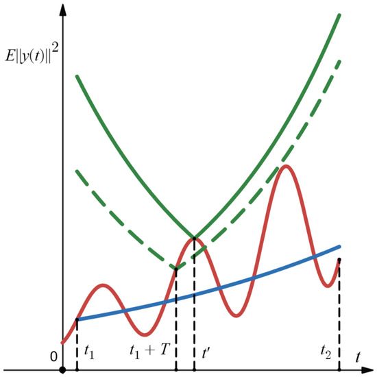
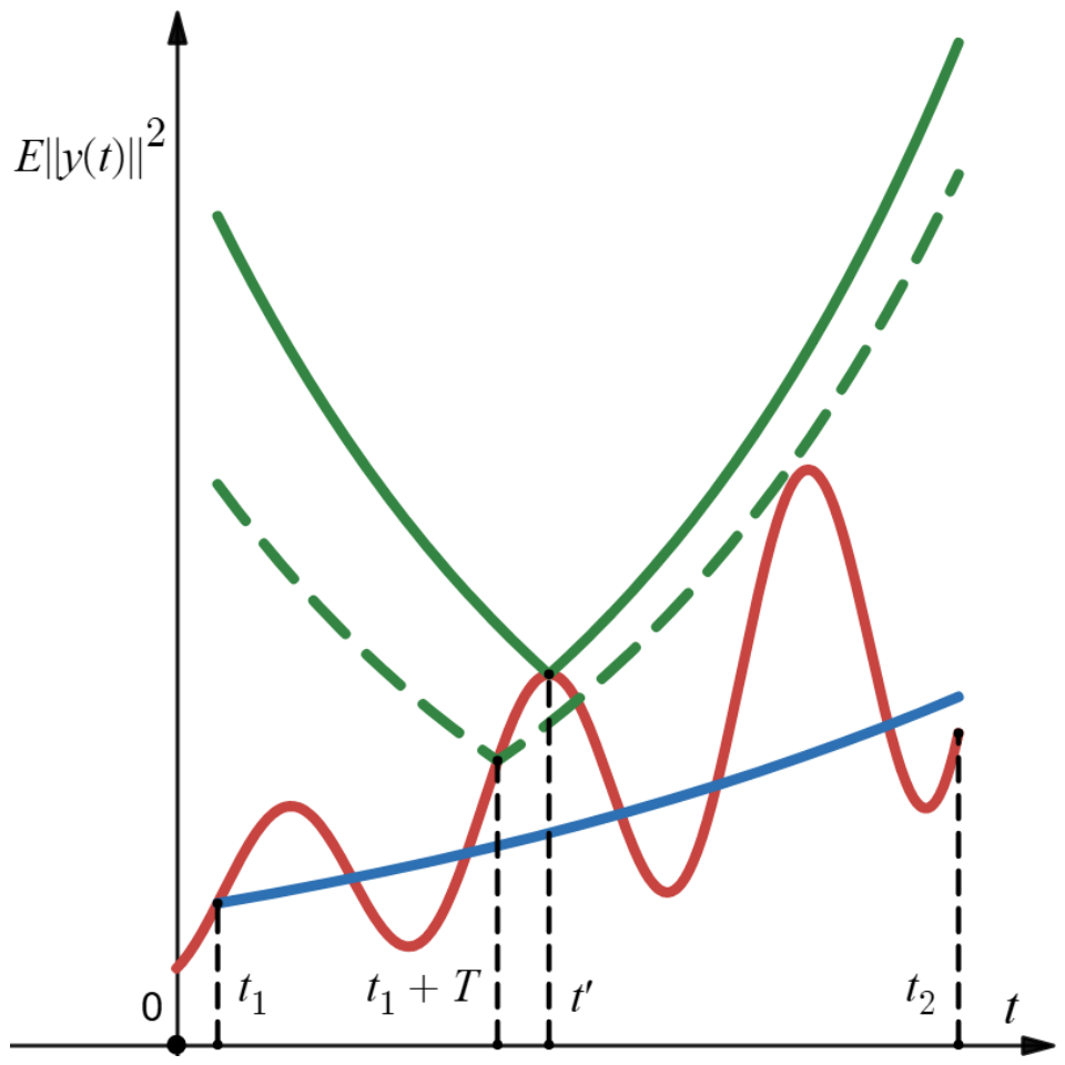
The algebraic details are somewhat involved, but the geometric idea is simple; for a clearer picture, see also Figure 1.

Figure 1. Illustration of Lemma 1. The red line is ${\mathbb{E}\parallel y\left(t\right)\parallel }^2$, and the blue line is the threshold $\mathbb{E}\parallel y\left(t_1\right){\parallel }^2{e}^{2\gamma (t-t_1)}$. Green curves illustrate the choice of $t^{\prime }$, such that $\mathbb{E}\parallel y\left(t^{\prime }\right){\parallel }^2{e}^{2{\alpha }^{\prime }|t-t^{\prime }|}\ge \mathbb{E}{\parallel y\left(t\right)\parallel }^2$.

Using the assumption for $t_1+T$ and the relation above (14), we obtain the following estimate at the point $t_2$:

$$\begin{array}{cc}\hfill \mathbb{E}\parallel y\left(t^{\prime }\right){\parallel }^2& \ge e^{2{\alpha }^{\prime }|t^{\prime }-(t_1+T)|}\mathbb{E}{\parallel y(t_1+T)\parallel }^2\hfill \\ \hfill & \ge e^{2{\alpha }^{\prime }|t^{\prime }-(t_1+T)|+2\gamma (t_1+T-t_2)}\mathbb{E}{\parallel y\left(t_2\right)\parallel }^2\hfill \\ \hfill & \ge e^{2({\alpha }^{\prime }-\left|\gamma \right|\left)\right|t^{\prime }-(t_1+T)|-2|\gamma \left|\right|t^{\prime }-t_2|}\mathbb{E}{\parallel y\left(t_2\right)\parallel }^2\hfill \\ \hfill & =e^{2({\alpha }^{\prime }-\left|\gamma \right|\left)\right|t^{\prime }-(t_1+T)|+2(\alpha -\left|\gamma \right|\left)\right|t^{\prime }-t_2|}{e}^{-2\alpha (t_2-t^{\prime })}\mathbb{E}{\parallel y\left(t_2\right)\parallel }^2\hfill \\ \hfill & \ge e^{2({\alpha }^{\prime }-\left|\gamma \right|)(t_2-(t_1+T))}{e}^{-2\alpha (t_2-t^{\prime })}\mathbb{E}{\parallel y\left(t_2\right)\parallel }^2.\hfill \end{array}$$

Hence

$$\mathbb{E}\parallel y\left(t^{\prime }\right){\parallel }^2{e}^{-2({\alpha }^{\prime }-|\gamma \left|\right)T}\ge e^{-2\alpha (t_2-t^{\prime })}\mathbb{E}{\parallel y\left(t_2\right)\parallel }^2.$$

(15)

A similar argument yields the estimate (15) at $t_1$:

$$\mathbb{E}\parallel y\left(t^{\prime }\right){\parallel }^2{e}^{-2({\alpha }^{\prime }-|\gamma \left|\right)T}\ge e^{-2\alpha (t^{\prime }-t_1)}\mathbb{E}{\parallel y\left(t_1\right)\parallel }^2.$$

(16)

From (14), we also get

$$\underset{t^{\prime }\le \tau \le t_2}{max}\mathbb{E}\left(\parallel y\left(\tau \right)e^{-{\alpha }^{\prime }(\tau -t^{\prime })}{\parallel }^2\right)=\underset{t_1\le \tau \le t^{\prime }}{max}\mathbb{E}\left(\parallel y\left(\tau \right)e^{-{\alpha }^{\prime }(t^{\prime }-\tau )}{\parallel }^2\right)=\mathbb{E}\left(\parallel y\left(t^{\prime }\right){\parallel }^2\right).$$

(17)

Using estimates (16) and (17), together with the inequality (13) applied on appropriate subintervals, we obtain

$$\mathbb{E}\left(\parallel y\left(t^{\prime }\right){\parallel }^2\right)\le 2C_0\mathbb{E}{\parallel y\left(t^{\prime }\right)\parallel }^2{e}^{-2({\alpha }^{\prime }-|\gamma \left|\right)T}+2{\beta }^{\prime }\mathbb{E}\left(\parallel y\left(t^{\prime }\right){\parallel }^2\right).$$

(18)

Now, choose ${\beta }^{\prime }$ and $t_0$, such that

$${\beta }^{\prime }<{\displaystyle \frac{1}{8}},$$

and take T satisfying

$$T>{\displaystyle \frac{ln\left(16N^2\right)}{2({\alpha }^{\prime }-|\gamma \left|\right)}}.$$

Then the inequality (18) contradicts the nontriviality of $\mathbb{E}\parallel y\left(t^{\prime }\right){\parallel }^2$, which proves the lemma. □

• Growth or decay in mean-square

Assume that $y\left(t\right)$ is a nontrivial solution to (1). Then, by Lemma 1, for any fixed $\gamma \mathrm{with}{\alpha }^{\prime }>\gamma >-{\alpha }^{\prime },$ there exists $t_0^{\prime }$, such that the graph of $\mathbb{E}(\parallel y\left(t\right){\parallel }^2)$ does not intersect the graph of $\mathbb{E}(\parallel y\left(t_1\right)e^{\gamma (t-t_1)}{\parallel }^2)$ for $t\ge t_0^{\prime }$. By continuity, for $t\ge t_0^{\prime }$, one of the inequalities

$$\mathbb{E}\left(\parallel y\left(t_1\right)e^{\gamma (t-t_1)}{\parallel }^2\right)<\mathbb{E}\left({\parallel y\left(t\right)\parallel }^2\right)\mathrm{or}\mathbb{E}\left(\parallel y\left(t_1\right)e^{\gamma (t-t_1)}{\parallel }^2\right)>\mathbb{E}\left({\parallel y\left(t\right)\parallel }^2\right)$$

holds for all $t\ge t_0^{\prime }$. The first case with $\gamma >0$ yields exponential growth; the second case with $\gamma <0$ yields exponential decay. It remains to rule out the possibility that the solution $y\left(t\right)$ is trapped between two exponentials with negative and positive exponents.

Fix $\gamma$ with $0<\gamma <{\alpha }^{\prime }$, and choose $t_0^{\prime }$ large enough so that the double inequality

$$\mathbb{E}\left({\parallel y\left(t_1\right)e^{-\gamma (t-t_1)}\parallel }^2\right)<\mathbb{E}\left({\parallel y\left(t\right)\parallel }^2\right)<\mathbb{E}\left(\parallel y\left(t_1\right)e^{\gamma (t-t_1)}{\parallel }^2\right),\mathrm{for}\mathrm{all}t>t_0^{\prime },$$

(19)

holds.

For any $\tau >t_0^{\prime }$ define

$$A_{\tau }=\{t\ge t_0^{\prime }{:\mathbb{E}\parallel y\left(\tau \right)\parallel }^2\le {\mathbb{E}\parallel y\left(t\right)\parallel }^2{e}^{-2{\alpha }^{\prime }|t-\tau |}\}.$$

Using (19), one shows that the set $A_{\tau }$ is bounded. Since ${\mathbb{E}\parallel y\left(t\right)\parallel }^2$ is continuous, the set $A_{\tau }$ is also closed and hence compact. Therefore, there exists a point ${\tau }^{\prime }\in A_{\tau }$ at which the maximum of ${\mathbb{E}\parallel y\left(t\right)\parallel }^2$ on $A_{\tau }$ is attained.

Moreover, for this choice of ${\tau }^{\prime }$, an argument analogous to that used in Lemma 1 (see also Figure 1) shows that ${\tau }^{\prime }$ is the only point in $A_{{\tau }^{\prime }}$, that is,

$$A_{{\tau }^{\prime }}=\left\{{\tau }^{\prime }\right\}.$$

(20)

Substituting $t_1=t_0^{\prime }$ and $t^{\prime }={\tau }^{\prime }$ into the projection estimate (13), using (19) and (20), and letting $t_2\to \infty$, we obtain

$$\begin{array}{cc}\hfill \mathbb{E}\left({\parallel y\left({\tau }^{\prime }\right)\parallel }^2\right)& \le C_0{e}^{-2\alpha ({\tau }^{\prime }-t_0^{\prime })}\mathbb{E}\left({\parallel y\left(t_0^{\prime }\right)\parallel }^2\right)+2{\beta }^{\prime }\mathbb{E}\left({\parallel y\left({\tau }^{\prime }\right)\parallel }^2\right)\hfill \\ & <\left(C_0{e}^{-2(\alpha -{\alpha }^{\prime })({\tau }^{\prime }-t_0^{\prime })}+2{\beta }^{\prime }\right)\mathbb{E}\left(\parallel y\left({\tau }^{\prime }\right){\parallel }^2\right).\hfill \end{array}$$

Choosing a sufficiently large ${\tau }^{\prime }$ yields a contradiction. This completes the proof.

• Final step: translation into Lyapunov characteristics

By the continuity of ${\mathbb{E}\parallel y\left(t\right)\parallel }^2$ and Lemma 1, for any fixed $\gamma \in (0,{\alpha }^{\prime })$, one of the following mutually exclusive alternatives holds, for all large t, for each nontrivial solution:

• ${\mathbb{E}\parallel y\left(t\right)\parallel }^2\ge \mathbb{E}{∥y\left(t_1\right)e^{\gamma (t-t_1)}∥}^2,$ which shows that ${\mathbb{E}\parallel y\left(t\right)\parallel }^2$ grows at least as $e^{2\gamma t}$ as $t\to \infty$. Moreover,

  $$\begin{array}{cc}\hfill {\underline{\lambda }}_2\left(y_0\right)& :={\displaystyle \frac{1}{2}}\underset{t\to \infty }{lim\; inf}{\displaystyle \frac{1}{t}}ln\mathbb{E}{\parallel y\left(t\right)\parallel }^2\ge {\displaystyle \frac{1}{2}}\underset{t\to \infty }{lim}{\displaystyle \frac{1}{t}}ln\mathbb{E}{∥y\left(t_1\right)e^{\gamma (t-t_1)}∥}^2\hfill \\ & =\underset{t\to \infty }{lim}{\displaystyle \frac{2\gamma (t-t_1)+ln\mathbb{E}{\parallel y\left(t_1\right)\parallel }^2}{2t}}=\gamma .\hfill \end{array}$$
  Hence, ${\underline{\lambda }}_2\left(y_0\right)\ge \gamma$. Since $\gamma \in (0,{\alpha }^{\prime })$ is arbitrary and intermediate growth rates are excluded by the previous analysis, it follows that ${\underline{\lambda }}_2\left(y_0\right)\ge {\alpha }^{\prime }$.
• Alternatively, ${\mathbb{E}\parallel y\left(t\right)\parallel }^2<\mathbb{E}{∥y\left(t_1\right)e^{\gamma (t-t_1)}∥}^2$. In this case, by the impossibility of intermediate growth established in (19), it follows that ${\mathbb{E}\parallel y\left(t\right)\parallel }^2\le \mathbb{E}{∥y\left(t_1\right)e^{-\gamma (t-t_1)}∥}^2.$ Hence, ${\mathbb{E}\parallel y\left(t\right)\parallel }^2$ decays at least as $e^{-2\gamma t}$ as $t\to \infty$.
  Proceeding in the same way, we conclude that ${\overline{\lambda }}_2\left(y_0\right)\le -\gamma$ and hence ${\overline{\lambda }}_2\left(y_0\right)\le -{\alpha }^{\prime }$.

We now return to the initial choice of ${\alpha }^{\prime }$. Because the preceding arguments apply for every ${\alpha }^{\prime }\in (0,\alpha )$, and the Lyapunov exponent is independent of this auxiliary parameter, we obtain the following bounds:

• For unbounded solutions, ${\overline{\lambda }}_2\left(y_0\right)\ge \alpha$.
• For bounded solutions, ${\overline{\lambda }}_2\left(y_0\right)\le -\alpha$.

This completes the proof of the theorem. □

Remark 3.

The assumption that the exponential dichotomy of A is given with a single rate $\alpha >0$ can be relaxed to admit distinct rates for the stable and unstable parts. More precisely, suppose there exist constants ${\alpha }_{-},{\alpha }_{+}>0$ and a bounded projection $P_{-}$, such that

$$\parallel P_{-}{e}^{As}\parallel \le N{e}^{-{\alpha }_{-}s},\parallel P_{+}{e}^{-As}\parallel \le N{e}^{-{\alpha }_{+}s},s\ge 0.$$

Then, under the remaining hypotheses of Theorem 1 (with the smallness condition in (H2) verified for sufficiently large times and with the perturbation amplitudes chosen small relative to ${\alpha }_{-}$ and ${\alpha }_{+}$), the conclusions of Theorem 1 hold with the rates applied separately to each spectral part, that is,

$${\overline{\lambda }}_2\left(y_0\right)\le -{\alpha }_{-}(forsolutionsboundedinmean\text{-}square),$$

and

$${\underline{\lambda }}_2\left(y_0\right)\ge {\alpha }_{+}(forsolutionswithanunboundedsecondmoment).$$

The proof is the same as that of Theorem 1, with the only difference that ${\beta }^{\prime }$ is replaced by $max\{{\beta }_{-},{\beta }_{+}\}$.

4. Examples

Here are examples illustrating Theorem 1.

Example 1.

Let $D\subset {\mathbb{R}}^d$ be a bounded domain with a sufficiently smooth boundary,

$$Au:=\sum _{i,j=1}^d{\left(a_{ij}\left(\xi \right)u_{{\xi }_i}\right)}_{{\xi }_j}=\mathrm{div}(a\left(\xi \right)\nabla u),$$

where $a\left(\xi \right)=\left(a_{ij}\left(\xi \right)\right)$ is a symmetric and bounded matrix, and $a_{ij}\left(\xi \right)$ are Hölder continuous with the Hölder exponent $\beta \in (0,1)$. Furthermore, assume there exists a constant $a_0>0$, such that

$$\left|⟨a\left(\xi \right)h,h⟩\right|\ge a_0{\parallel h\parallel }^2,$$

for all $\xi \in D$ and $h\in {\mathbb{R}}^d$. The boundedness of $A\left(\xi \right)$ implies that there exists $a_1>0$, such that

$$\left|⟨a\left(\xi \right)h,h⟩\right|\le a_1{\parallel h\parallel }^2.$$

Set $H=L^2\left(D\right)$. It is well known that the operator A generates a $C_0$-semigroup $S\left(t\right)=e^{At}\in H$, and has a discrete spectrum: a sequence of eigenvalues

$$0<{\lambda }_1\le {\lambda }_2\le \dots \le {\lambda }_n\le \dots ,{\lambda }_n\to \infty ,asn\to \infty .$$

Let $\left\{e_n\right\}$ be the corresponding orthonormal eigenbasis in H, such that

$$\underset{n\in N}{sup}{\parallel e_n\parallel }_{L^{\infty }\left(D\right)}<\infty .$$

According to standard results (see, e.g., [14]), such a basis always exists.

Let ${\mu }_n\ge 0$, ${\sum }_{n=1}^{\infty }{\mu }_n<\infty$, and we introduce the covariance operator $Q\in \mathcal{L}\left(H\right)$, such that Q is non-negative, $\mathrm{Tr}\left(Q\right)<\infty$, and $Q{e}_n={\mu }_n{e}_n$.

This allows us to define an H-valued stochastic process

$$W\left(t\right):=\sum _{n=1}^{\infty }\sqrt{{\mu }_n}{e}_n\left(\xi \right){\beta }_n\left(t\right),t\ge 0,$$

which is a Q-Wiener process. Here, ${\beta }_n\left(t\right)$ are standard, scalar, mutually independent Wiener processes. Denote $U:=Q^{{\displaystyle \frac{1}{2}}}\left(L^2\left(D\right)\right)$. It follows from ([15], Lemma 2.2), that $U\subset L^{\infty }\left(D\right)$. For any fixed $\varphi \in L^2\left(D\right)$, we may now introduce the multiplication operator $\mathsf{\Phi }:U\to H$ defined by

$$\mathsf{\Phi }\left(\varphi \right):=\varphi ·\psi ,\forall \psi \in U.$$

Since $\psi \in L^2\left(D\right)$ and $\varphi \in L^{\infty }\left(D\right)$, the operator $\mathsf{\Phi }$ is well defined. Hence $\mathsf{\Phi }\circ Q^{1/2}:L^2\left(D\right)\to L^2\left(D\right)$ is a Hilbert–Schmidt operator.

In the sequel, we denote by $L_2^0=L_2(Q^{1/2}H,H)$ the space of Hilbert–Schmidt operators with the norm ${\parallel ·\parallel }_{HS}$. Then

$$\begin{array}{cc}\hfill {\parallel \mathsf{\Phi }\circ Q^{1/2}\parallel }_{HS}^2& :=\sum _{i=1}^{\infty }{\parallel \mathsf{\Phi }\circ Q^{1/2}{e}_i\parallel }^2=\sum _{i=1}^{\infty }{\mu }_i{\int }_D\varphi {\left(\xi \right)}^2{e}_i^2\left(\xi \right)d\xi \hfill \\ & \le \mathrm{Tr}\left(Q\right)\underset{i}{sup}\parallel e_i{\parallel }_{L^{\infty }\left(D\right)}^2·{\parallel \varphi \parallel }_{L^2\left(D\right)}^2.\hfill \end{array}$$

Hence, if $\mathsf{\Phi }:\mathsf{\Omega }\times [0,T]\to L(U,H)$ is a predictable process, such that

$$\mathbb{E}{\int }_0^T{\parallel \mathsf{\Phi }\left(s\right)Q^{1/2}\parallel }_{HS}^{2}ds<\infty ,$$

then, following [15], we can define the stochastic integral

$${\int }_0^t\mathsf{\Phi }\left(s\right)dW\left(s\right)\in H,$$

$${\int }_0^t\mathsf{\Phi }\left(s\right)dW\left(s\right)=\sum _{i=1}^{\infty }\sqrt{{\mu }_i}{\int }_0^t\mathsf{\Phi }(s,·)e_i(·)d{\beta }_i\left(s\right),$$

and

$$\mathbb{E}{\left|{\int }_0^t\mathsf{\Phi }\left(s\right)dW\left(s\right)\right|}^2\le \mathrm{Tr}\left(Q\right)\underset{i}{sup}\parallel e_i{\parallel }_{L^{\infty }\left(D\right)}^2{\int }_0^t\mathbb{E}{\left|\varphi (s,·)\right|}^{2}ds.$$

We consider the following stochastic linear partial differential equation:

$$\left\{\begin{array}{c}{\displaystyle dX(t,\xi )=\left(\sum _{i,j=1}^d{\left(a_{ij}\left(\xi \right)X_{{\xi }_i}\right)}_{{\xi }_j}+\lambda X(t,\xi )\right)dt+\sum _{n=1}^{\infty }\sqrt{{\mu }_n}{p}_n(t,\xi ,X)d{\beta }_n\left(t\right),}\hfill \\ {\displaystyle X(t,\xi ){|}_{\xi \in \partial D}=0,}\hfill \end{array}\right.$$

(21)

where the function $p(t,\xi ,X)=\sqrt{{\sum }_{n=1}^{\infty }{p_n}^2(t,\xi ,X)}$ is Lipschitz continuous for $t\ge 0$, $\xi \in D$, and ${sup}_{\xi \in D}p(t,\xi ,X)\to 0$, as $t\to \infty$. The parameter $\lambda >0$ is chosen, such that $\lambda \ne {\lambda }_j,\mathrm{for}\mathrm{all}j=1,2,\dots$.

Then, obviously, all the conditions of Theorem 1 are fulfilled, and the mean-square Lyapunov exponents of Equation (21) are preserved (i.e., they coincide with the reference exponents of the linear part).

In the following example, we consider the one-dimensional problem (21) with $A=\Delta$. In this case, the spectrum is given explicitly.

Example 2.

Let $D=(0,\pi )$. Consider the problem

$$\left\{\begin{array}{c}dX(t,\xi )=\left({\Delta }_{\xi }X(t,\xi )+\lambda X(t,\xi )\right)dt\hfill \\ {\displaystyle +\sum _{n=1}^{\infty }\sqrt{{\mu }_n}{p}_n(t,\xi ,X)e_n\left(\xi \right)d{\beta }_n\left(t\right),}\hfill \\ X(t,0)=X(t,\pi )=0,t\ge 0,\hfill \end{array}\right.$$

(22)

$\lambda >0$, $\lambda \ne n^2$, $n\in \mathbb{N}$. The function $p(t,\xi ,X)$ satisfies the previous conditions. In this case, $H=L^2(0,\pi )$, and the operator $A={\displaystyle \frac{d^2}{d{\xi }^2}}+\lambda I$, with $D\left(A\right)=H^2(0,\pi )\cap H_0^1(0,\pi )$.

Then, as is well known [16], the spectrum

$$\sigma \left(A\right)=\{\lambda -n^2:n\in \mathbb{N}\}$$

is real and $0\notin \sigma \left(A\right)$. Set

$${\alpha }_{+}:=\underset{n^2<\lambda }{min}(\lambda -n^2),{\alpha }_{-}:=\underset{n^2>\lambda }{min}(n^2-\lambda ).$$

Then ${\alpha }_{+},{\alpha }_{-}>0$ and $\alpha =min\{{\alpha }_{+},{\alpha }_{-}\}$.

For any mild solution $y(t;y_0)$ of (22), Theorem 1 implies:

1.

If the solution has an unbounded second moment, then

$${\underline{\lambda }}_2\left(y_0\right)\ge \alpha .$$

2.

If the solution has a bounded second moment, then

$${\overline{\lambda }}_2\left(y_0\right)\le -\alpha .$$

Thus, on the unstable spectral subspace, the mean-square Lyapunov exponent is not smaller than the minimal positive eigenvalue ${\alpha }_{+}$, while on the stable subspace, it does not exceed the negative of the minimal modulus of the negative eigenvalues, $-{\alpha }_{-}$.

Remark 4.

Inspecting the proof of Theorem 1, one can see that, if necessary, the exact rates ${\alpha }_{+}$ and ${\alpha }_{-}$ can be taken instead of the common value α.

5. Discussion

This paper studies the Lyapunov structure of nonlinear stochastic evolution equations in a separable Hilbert space driven by a Q-Wiener process. The linear operator A generates a $C_0$-semigroup admitting an exponential dichotomy, which induces a splitting associated with positive and negative Lyapunov exponents. The nonlinear drift and diffusion terms are assumed to be globally Lipschitz and to decay in time.

The main result shows that the Lyapunov exponents of the nonlinear stochastic equation coincide with those of the linear part. In particular, no new mean-square growth rates appear due to the nonlinear perturbations, and the splitting induced by the operator A remains unchanged in the mean-square sense.

The analysis confirms that the linear exponential dichotomy provides a correct reference structure for the nonlinear stochastic system and that this structure is robust under small fading perturbations in both drift and diffusion terms. The proof relies on the spectral splitting of the semigroup generated by A and on mean-square estimates based on the Itô isometry.

From a physical viewpoint, assumption (H2) means that the nonlinear perturbation vanishes at the equilibrium state: indeed, $F(t,0)=0$ and $G(t,0)=0$ for all $t\ge 0$, so the system contains no additive forcing at the origin. In this sense, the nonlinear terms act only as state-dependent perturbations, which is consistent with a model of fading or self-regulating effects rather than external noise injected independently of the current state. The nonautonomous character of the coefficients is also natural in applications, since it allows the strength of the perturbation to change in time while still remaining asymptotically negligible.

We also remark that condition (H2) could likely be weakened to a more physically natural growth bound of the form $\parallel F(t,y)\parallel +{\parallel G(t,y)\parallel }_{HS}\le C(1+\parallel y\parallel ),$ or to a similar subcritical condition. Such a refinement would broaden the range of admissible models, but it would require additional technical estimates in the proof. On the other hand, assumption (H1) can probably be relaxed without essential difficulty; it is imposed here mainly to keep the statement and the exposition as transparent as possible.

The obtained results give a simple and verifiable criterion for the invariance in Lyapunov exponents in nonlinear stochastic evolution equations. Possible extensions include weaker decay conditions and almost-sure versions of the obtained statements.

References

- Daleckii, J.L.; Krein, M.G. Stability of Solutions of Differential Equations in Banach Space; American Mathematical Society: Providence, RI, USA, 1974; p. 386. [Google Scholar]
- Stanzhytskyi, O. Investigation of exponential dichotomy of Ito stochastic systems by using quadratic forms. Ukr. Math. J. 2001, 53, 1882–1894. [Google Scholar] [CrossRef] [Scilit]
- Stanzhytskyi, O. Exponential dichotomy and mean-square bounded solutions of linear stochastic Ito systems. Nonlinear Oscil. 2001, 4, 389–398. [Google Scholar]
- Samoilenko, A.M.; Stanzhytskyi, O.M. Qualitative and Asymptotic Analysis of Differential Equations with Random Perturbations; World Scientific: Singapore, 2011; p. 322. [Google Scholar]
- Ungureanu, V.M. Representation theorem for stochastic differential equations in Hilbert spaces and its applications. Surv. Math. Its Appl. 2006, 1, 117–134. [Google Scholar]
- Stoica, D. Uniform exponential dichotomy of stochastic cocycles. Stoch. Processes Their Appl. 2010, 120, 1920–1928. [Google Scholar] [CrossRef] [Scilit]
- Arnold, L.; Kliemann, W.; Oeljeklaus, E. Lyapunov exponents of linear stochastic systems. In Lyapunov Exponents; Ludwig, A., Wihstutz, V., Eds.; Springer: Berlin/Heidelberg, Germany, 1986; pp. 85–125. [Google Scholar]
- Arnold, L.; Papanicolaou, G.; Wihstutz, V. Asymptotic analysis of the Lyapunov exponent and rotation number of the random oscillator and applications. SIAM J. Appl. Math. 1986, 46, 427–450. [Google Scholar] [CrossRef] [Scilit]
- Baxendale, P.H. Lyapunov exponents and shear-induced chaos for a Hopf bifurcation with additive noise. Probab. Theory Relat. Fields 2024, 193, 375–425. [Google Scholar] [CrossRef] [Scilit]
- Bedrossian, A.; Blumenthal, A.; Punshon-Smith, S. Lower bounds on the Lyapunov exponents of stochastic differential equations. In International Congress of Mathematicians; EMS Press: Berlin, Switzerland, 2023; Volume 7, pp. 5618–5654. [Google Scholar]
- Barreira, L.; Valls, C. Stability of Nonautonomous Differential Equations; Lecture Notes in Mathematics; Springer: Berlin/Heidelberg, Germany, 2008; Volume 1926. [Google Scholar]
- Flandoli, F.; Gess, B.; Scheutzow, M. Synchronization by noise. Probab. Theory Relat. Fields 2017, 168, 511–556. [Google Scholar] [CrossRef] [Scilit]
- Prato, G.D.; Zabczyk, J. Stochastic Equations in Infinite Dimensions, 2nd ed.; Cambridge University Press: Cambridge, UK, 2014. [Google Scholar]
- Ovsepian, R.I.; Pelczynski, A. On the existence of a fundamental total biorthogonal sequence in every separable Banach space and related constructions of uniformly bounded orthonormal systems in L2. Stud. Math. 1975, 54, 149–159. [Google Scholar] [CrossRef] [Scilit]
- Manthey, R.; Zausinger, T. Stochastic evolution in . Stochastics Stochastics Rep. 1999, 66, 37–85. [Google Scholar] [CrossRef] [Scilit]
- Evans, L.C. Partial Differential Equations, 2nd ed.; American Mathematical Society: Providence, RI, USA, 2010. [Google Scholar]
Disclaimer/Publisher’s Note: The statements, opinions and data contained in all publications are solely those of the individual author(s) and contributor(s) and not of MDPI and/or the editor(s). MDPI and/or the editor(s) disclaim responsibility for any injury to people or property resulting from any ideas, methods, instructions or products referred to in the content. |
© 2026 by the authors. Licensee MDPI, Basel, Switzerland. This article is an open access article distributed under the terms and conditions of the Creative Commons Attribution (CC BY) license.