A Class of Causal 2D Markov-Switching ARMA Models: Probabilistic Properties and Variational Estimation

Abstract

This paper introduces a rigorous class of two-dimensional Markov-switching autoregressive moving-average (2D MS-ARMA) models for spatial lattice data exhibiting regime-dependent dynamics. The switching mechanism is governed by a latent causal Markov random field that drives spatial transitions between regime-specific autoregressive and moving-average structures. We provide sufficient conditions for the existence of a strictly stationary solution through the top Lyapunov exponent associated with a sequence of random matrices obtained from a state-space representation constructed along the lexicographic order. For the first-order bidirectional specification, we derive explicit spectral conditions linking stationarity to the regime-dependent spectral radii. Sufficient conditions ensuring the existence of finite second-order moments are also provided. Parameter estimation is carried out using a variational expectation–maximization (VEM) algorithm based on a mean-field approximation of the posterior distribution of the hidden regimes. The E-step yields closed-form coordinate ascent updates, while the M-step relies on gradient-based numerical optimization with derivatives computed via recursive differentiation. Under increasing-domain asymptotics, we discuss the consistency and asymptotic behavior of the variational estimator. The proposed framework fills a methodological gap between classical one-dimensional Markov-switching ARMA models and spatial autoregressive structures by extending regime-switching theory to multi-indexed processes with rigorous probabilistic foundations. It provides a comprehensive basis for statistical inference, model diagnostics, and prediction in spatially heterogeneous environments.

1. Introduction

Autoregressive moving average (ARMA) models form a cornerstone of stochastic process modeling, providing parsimonious representations of stationary dynamics and effective forecasting tools [1]. In many applications, however, the underlying mechanism exhibits structural changes or regime-dependent behavior that cannot be captured by a single global specification. Classical examples include business cycle phases in macroeconomic series [2], heterogeneous spatial patterns in images [3], and locally unstable economic indicators.

Markov-switching (MS) models address this issue by allowing parameters to evolve according to an unobserved latent Markov process. Since the seminal contribution of Hamilton [2], MS autoregressive and ARMA models have been extensively developed. Foundational results on stationarity and covariance structure were established by Francq and Zakoïan [4] and refined in Francq and Zakoïan [5] and Pataracchia [6]. Modern developments include Bayesian formulations [7], Markov-switching spatio-temporal ARCH models [8], and inference under weak dependence [9], supported by advances in hidden Markov model theory [10].

Recent advances in machine learning have proposed flexible predictive and generative models for structured data, including GAN-based approaches for tabular imputation and ensemble methods for prediction tasks. While these methods focus on predictive accuracy, they typically do not provide a probabilistic framework for inference in spatially dependent time series models. The present work complements this literature by developing a theoretically grounded approach based on stochastic recurrence equations and regime-switching spatial processes.

More broadly, recent contributions have also addressed latent heterogeneity and structured dependence in related settings. For example, functional-coefficient quantile regression models for panel data with latent group structures have been proposed to capture heterogeneous effects under dependence [11]. Similarly, graph-based approaches to structured dependence and partitioning have been developed to model complex heterogeneous systems [12].

From a probabilistic viewpoint, strict stationarity and moment existence rely on Lyapunov exponent techniques and products of random matrices. The foundational work of Bougerol and Picard [13] established sharp stability criteria for random coefficient autoregressive processes, later extended to MS-ARMA frameworks by Stelzer [14] and related studies [15,16]. A crucial insight is that regime-wise stability does not ensure global stationarity. Nevertheless, these results are almost exclusively restricted to one-dimensional time-indexed Markov chains.

Parallel developments in spatial statistics have extended autoregressive modeling to two-dimensional settings. Early spatial interaction models were proposed by Kashyap and Chellappa [17], while spatial econometric formulations were developed in Fingleton [18] and Holly et al. [19]; see also Cressie and Wikle [20] and LeSage and Pace [21]. However, these models assume spatial homogeneity. The need for multidimensional stochastic modeling with rigorous asymptotic foundations has been highlighted in related contexts, such as inference for two-dimensional GARCH processes [22] and local asymptotic distribution theory for regime-switching structures [23].

A first step toward spatial regime modeling was made by Djafri and Kharfouchi [3], who introduced a two-dimensional Markov-switching autoregressive (2D MS-AR) model driven by a causal Markov random field and estimated via a variational EM algorithm. Despite its practical relevance, several theoretical aspects remain unresolved. In particular, the stationarity condition is not formulated in terms of Lyapunov exponents, the model excludes moving average components, and explicit moment conditions required for asymptotic inference are not established.

The present work fills this gap by introducing a general class of two-dimensional Markov-switching ARMA models whose regimes evolve according to a causal Markov random field on a lattice. Our contributions are threefold. First, we provide sufficient conditions for the existence of a strictly stationary solution via the top Lyapunov exponent of an associated random matrix product, thereby extending classical one-dimensional MS-ARMA theory to spatially indexed processes. Second, we derive explicit spectral conditions for first-order bidirectional specifications. Third, we provide sufficient conditions for the existence of second-order moments, which are essential for likelihood-based estimation and asymptotic analysis.

Unlike classical MS-ARMA models where regimes evolve along a linear time axis, the regime process in our framework exhibits spatial dependence. We show that Kingman’s subadditive ergodic theorem remains applicable under stationarity and ergodicity of the Markov random field, providing a rigorous probabilistic foundation for inference in spatially regime-dependent ARMA models.

The remainder of the paper is organized as follows. Section 2 introduces the model formulation and develops the state–space representation together with the associated stationarity conditions based on the Lyapunov exponent.

Section 3 presents the variational estimation procedure, including the EM-type algorithm and the asymptotic properties of the estimators.

Section 4 contains simulation studies and an empirical application, illustrating the finite-sample performance of the proposed method and the impact of spatial dependence.

2. Model Formulation and State–Space Representation

Let $S\subset {\mathbb{Z}}^2$ be a finite endowed with the lexicographic order ≺, defined for $t=(t_1,t_2)$ and $s=(s_1,s_2)$ in ${\mathbb{Z}}^2$ by

$$t\prec s\mathrm{if}{t}_1<s_1\mathrm{or}(t_1=s_1\mathrm{and}{t}_2<s_2).$$

Let ${\left(Z_t\right)}_{t\in S}$ be a finite–state homogeneous first–order causal Markov random field with state space $\mathrm{\Lambda }=\{1,\dots ,L\}$. We assume that $\left(Z_t\right)$ is strictly stationary and ergodic with respect to spatial translations in ${\mathbb{Z}}^2$.

Let ${\left({\epsilon }_t\right)}_{t\in S}$ be an i.i.d. sequence of real random variables defined on a complete probability space $(\Omega ,\mathcal{F},\mathbb{P})$ such that

$$\mathbb{E}\left[{\epsilon }_t\right]=0,\mathbb{E}{log}^{+}\left|{\epsilon }_t\right|<\infty ,$$

and assume that $\left({\epsilon }_t\right)$ is independent of $\left(Z_t\right)$.

For $p=(p_1,p_2)$ and $q=(q_1,q_2)$, define the index sets

$$S]0,p]=\{k\in S:0\prec k⪯p\},S]0,q]=\{h\in S:0\prec h⪯q\}.$$

Since S is a finite index set, the sets $S]0,p]$ and $S]0,q]$ are also finite.

Definition 1.

The random field ${\left(Y_t\right)}_{t\in S}$ is said to follow a causal 2D Markov–Switching ARMA$(p,q)$ model if for all $t\in S$,

$$Y_t=\mu \left(Z_t\right)+\sum _{k\in S]0,p]}{a}_k\left(Z_t\right)Y_{t-k}+\sum _{h\in S]0,q]}{b}_h\left(Z_t\right){\epsilon }_{t-h}+{\epsilon }_t,$$

(1)

where $\mu (·)$, $a_k(·)$ and $b_h(·)$ are real–valued functions defined on Λ. The model is said to be causal in the sense that $Y_t$ depends only on past values $Y_s$ and ${\epsilon }_s$ with $s\prec t$.

Remark 1.

The adoption of a lexicographic ordering ≺ on ${\mathbb{Z}}^2$ facilitates a causal recursive structure, transforming the 2D dependence into a 1D sequence. While this approach prioritizes a specific directional flow and departs from spatial isotropy, it is a well-established and standard convention for 2D stochastic processes in the field of image processing [24,25]. In this context, such a unilateral representation is essential as it enables the use of computationally efficient recursive estimation, stability analysis via Lyapunov exponents, and state-space filtering that would otherwise be intractable in purely bilateral spatial models.

2.1. State—Space Representation

To study strict stationarity, we rewrite the model in state—space form. Let $r=\max (p_1,q_1)$ and $s=\max (p_2,q_2)$ and define

$$d=2(r+1)(s+1).$$

Define the state vector $X_t\in {\mathbb{R}}^d$ by stacking current and lagged values of $\left(Y_t\right)$ and $\left({\epsilon }_t\right)$ in lexicographic order so that the recursion becomes first–order Markovian along the lexicographic path.

For every $t\in S$ that is not minimal with respect to ≺, define its immediate predecessor with respect to ≺ as

$$t^{-}=\max \{s\in S:s\prec t\},$$

whenever this set is nonempty. Since ≺ is a total order on S, this predecessor is uniquely defined whenever it exists.

A companion–form construction yields measurable random matrices $\mathcal{A}\left(Z_t\right)\in {\mathbb{R}}^{d\times d}$ and $\mathcal{B}\left(Z_t\right)\in {\mathbb{R}}^d$ such that (1) is equivalent to

$$X_t=\mathcal{A}\left(Z_t\right)X_{t^{-}}+\mathcal{B}\left(Z_t\right){\epsilon }_t.$$

(2)

2.2. Probabilistic Framework and Matrix Products

To analyze stability and stationarity of the recursion (2), we formalize the probabilistic structure of the random matrix products generated along the lexicographic path.

Let $(\Omega ,\mathcal{F},\mathbb{P})$ support the strictly stationary process ${(Z_t,{\epsilon }_t)}_{t\in S}$ with respect to spatial translations in ${\mathbb{Z}}^2$. Fix an arbitrary site $t_0\in S$ and construct a sequence ${\left(t_n\right)}_{n\ge 0}$ recursively by

$$t_{n+1}=t_n^{-},$$

whenever the predecessor exists. This defines a path into the past along the lexicographic ordering.

For $n\ge 1$, define the random matrix products

$${\Phi }_n=\mathcal{A}\left(Z_{t_1}\right)\mathcal{A}\left(Z_{t_2}\right)\dots \mathcal{A}\left(Z_{t_n}\right),{\Phi }_0=I_d.$$

By submultiplicativity of the matrix norm, for all $m,n\ge 1$,

$$\parallel {\Phi }_{m+n}\parallel \le \parallel {\Phi }_m\parallel ∥\mathcal{A}\left(Z_{t_{m+1}}\right)\dots \mathcal{A}\left(Z_{t_{m+n}}\right)∥,$$

which implies that the sequence

$$X_n=log\parallel {\Phi }_n\parallel$$

is subadditive along the lexicographic path.

Assume:

• (A1) $\left(Z_t\right)$ is strictly stationary and ergodic,
• (A2) $\mathbb{E}{log}^{+}\parallel \mathcal{A}\left(Z_t\right)\parallel <\infty$,
• (A3) $\mathbb{E}{log}^{+}\parallel \mathcal{B}\left(Z_t\right)\parallel <\infty$.

Then $\left(X_n\right)$ satisfies the integrability and subadditivity conditions required by Kingman’s subadditive ergodic theorem. Consequently, the limit defining the top Lyapunov exponent exists almost surely.

We assume that the model is quadrant-causal with respect to the lexicographic order ≺, in the sense that all autoregressive and moving-average coefficients satisfy

$${\Phi }_k\left(Z_t\right)=0\mathrm{for}\mathrm{all}k⪯0,$$

so that $X_t$ depends only on past indices $t_k\prec t$. This ensures that the field admits a recursive representation along the lexicographic path.

Lemma 1

(Existence of the Lyapunov exponent). Under Assumptions (A1)–(A2), and under the quadrant-causality assumption ensuring a unilateral recursion along the lexicographic path, the sequence ${\left\{\mathcal{A}\left(Z_{t_n}\right)\right\}}_{n\ge 1}$ is stationary and ergodic along the path. Consequently, the limit

$$\gamma =\underset{n\to \infty }{\lim }{\displaystyle \frac{1}{n}}log\parallel {\Phi }_n\parallel$$

exists almost surely and in $L^1$, and is constant $\mathbb{P}$–almost surely.

Proof. 

Let ${\left(t_n\right)}_{n\ge 0}$ be the sequence of sites constructed by repeated application of the predecessor operator, $t_{n+1}=t_n^{-}$, starting from an arbitrary $t_0\in S$.

By the quadrant-causality assumption, the predecessor mapping induces a strictly unilateral (non-anticipative) ordering of the lattice. This ordering defines a shift operator $\theta$ acting on the canonical probability space by

$$\theta \left(\omega \right)=(Z_{t_1},Z_{t_2},\dots ).$$

Under Assumption (A1), the random field $\left(Z_t\right)$ is strictly stationary and ergodic, which implies that $\theta$ is measure-preserving and ergodic.

Define, for $n\ge 1$,

$${\Phi }_n=\mathcal{A}\left(Z_{t_1}\right)\mathcal{A}\left(Z_{t_2}\right)\cdots \mathcal{A}\left(Z_{t_n}\right),{\Phi }_0=I_d,$$

and set

$$X_n=log\parallel {\Phi }_n\parallel .$$

• Subadditivity.

For all $m,n\ge 1$, by submultiplicativity of the matrix norm,

$$\parallel {\Phi }_{m+n}\parallel \le \parallel {\Phi }_m\parallel ∥\mathcal{A}\left(Z_{t_{m+1}}\right)\cdots \mathcal{A}\left(Z_{t_{m+n}}\right)∥.$$

Taking logarithms yields

$$X_{m+n}\le X_m+X_n\circ {\theta }^m,$$

where ${\theta }^m$ denotes the m-fold shift. By stationarity of $\left(Z_t\right)$, the sequence $(X_n\circ {\theta }^m)$ has the same distribution as $\left(X_n\right)$.

• Integrability.

Assumption (A2) ensures that

$$\mathbb{E}{log}^{+}\parallel \mathcal{A}\left(Z_{t_0}\right)\parallel <\infty ,$$

which implies $\mathbb{E}|X_1|<\infty$. Moreover,

$$X_n\le \sum _{k=1}^n{log}^{+}\parallel \mathcal{A}\left(Z_{t_k}\right)\parallel ,$$

so that $\mathbb{E}|X_n|<\infty$ for all n.

• Application of Kingman’s theorem.

The sequence $\left(X_n\right)$ is subadditive, integrable, and adapted to the measure-preserving and ergodic transformation $\theta$. Therefore, Kingman’s subadditive ergodic theorem applies and yields

$$\underset{n\to \infty }{\lim }{\displaystyle \frac{1}{n}}{X}_n=\underset{n\ge 1}{\inf }{\displaystyle \frac{1}{n}}\mathbb{E}\left[X_n\right]\mathrm{almost}\mathrm{surely}\mathrm{and}\mathrm{in}{L}^1.$$

Consequently,

$$\gamma =\underset{n\to \infty }{\lim }{\displaystyle \frac{1}{n}}log\parallel {\Phi }_n\parallel$$

exists almost surely, is finite, and is deterministic. □

Theorem 1

(Existence of a strictly stationary causal solution). Consider the state–space recursion

$$X_t=\mathcal{A}\left(Z_t\right)X_{t^{-}}+\mathcal{B}\left(Z_t\right){\epsilon }_t,$$

defined in (2). Under Assumptions (A1)–(A3), if the top Lyapunov exponent

$$\gamma =\underset{n\to \infty }{\lim }{\displaystyle \frac{1}{n}}log\parallel {\Phi }_n\parallel$$

satisfies $\gamma <0$, then there exists a unique strictly stationary and causal solution ${\left(X_t\right)}_{t\in S}$ given by the almost surely convergent series

$$X_t=\sum _{k=0}^{\infty }{\Phi }_k\left(t\right)\mathcal{B}\left(Z_{t_k}\right){\epsilon }_{t_k},$$

(3)

where, for each site $t\in S$, ${\Phi }_k\left(t\right)$ denotes the product of coefficient matrices along the backward lexicographic path starting from t, that is,

$${\Phi }_k\left(t\right)=\mathcal{A}\left(Z_{t_1}\right)\cdots \mathcal{A}\left(Z_{t_k}\right),$$

ensuring a strictly non-anticipative (unilateral) recursion.

Proof. 

Fix an arbitrary site $t\in S$ and construct the backward path ${\left(t_k\right)}_{k\ge 0}$ defined by $t_0=t$ and $t_{k+1}=t_k^{-}$.

• Step 1: Finite expansion.

By repeated substitution of the recursion (2), for any $N\ge 1$ we obtain

$$X_t={\Phi }_N\left(t\right)X_{t_N}+\sum _{k=0}^{N-1}{\Phi }_k\left(t\right)\mathcal{B}\left(Z_{t_k}\right){\epsilon }_{t_k}.$$

(4)

• Step 2: Exponential decay of products.

By Lemma 1,

$$\underset{n\to \infty }{\lim }{\displaystyle \frac{1}{n}}log\parallel {\Phi }_n\parallel =\gamma \mathrm{a}.\mathrm{s}.$$

If $\gamma <0$, then for any $\eta \in (0,-\gamma )$ there exists $N_0\left(\omega \right)$ such that for all $n\ge N_0\left(\omega \right)$,

$$\parallel {\Phi }_n\parallel \le e^{-n\eta }\mathrm{almost}\mathrm{surely}.$$

• Step 3: Convergence of the series.

Using submultiplicativity,

$$\parallel {\Phi }_k\left(t\right)\mathcal{B}\left(Z_{t_k}\right){\epsilon }_{t_k}\parallel \le \parallel {\Phi }_k\left(t\right)\parallel \parallel \mathcal{B}\left(Z_{t_k}\right)\parallel |{\epsilon }_{t_k}|.$$

By Assumption (A3),

$$\mathbb{E}{log}^{+}\parallel \mathcal{B}\left(Z_t\right)\parallel <\infty ,\mathbb{E}{log}^{+}\left|{\epsilon }_t\right|<\infty .$$

Combined with the exponential decay of $\parallel {\Phi }_k\left(t\right)\parallel$, this implies that the series

$$\sum _{k=0}^{\infty }\parallel {\Phi }_k\left(t\right)\parallel \parallel \mathcal{B}\left(Z_{t_k}\right)\parallel |{\epsilon }_{t_k}|$$

converges almost surely by standard results on stochastic recurrence equations with negative Lyapunov exponent (see, e.g., [13], Theorem 2.1).

Therefore, the series in (3) converges absolutely almost surely and defines a candidate solution.

We emphasize that existence of the solution is obtained directly from the convergence of the series, independently of the finite expansion (4). In particular, no boundedness assumption on $X_t$ is required.

• Step 4: Verification of the recursion.

The series representation (3) satisfies the state–space recursion by direct substitution and index shifting, hence it defines a solution to (2).

• Step 5: Stationarity.

Since $(Z_t,{\epsilon }_t)$ is strictly stationary and the coefficients ${\Phi }_k\left(t\right)$ depend only on relative shifts along the lexicographic path, the mapping from $(Z,\epsilon )$ to $X_t$ is shift-invariant. Therefore, $\left(X_t\right)$ is strictly stationary.

• Step 6: Uniqueness.

Let $\left({\tilde{X}}_t\right)$ be another causal solution. Then the difference $D_t=X_t-{\tilde{X}}_t$ satisfies

$$D_t=\mathcal{A}\left(Z_t\right)D_{t^{-}}.$$

Iterating along the path yields

$$D_t={\Phi }_n\left(t\right)D_{t_n}.$$

Taking norms and using the exponential decay of ${\Phi }_n\left(t\right)$ implies $\parallel D_t\parallel \to 0$ almost surely, hence $D_t=0$, establishing uniqueness. □

2.3. Invertibility and Recovery of the Innovation Sequence

In addition to strict stationarity, the practical use of the model requires invertibility, that is, the possibility of recovering the innovation sequence from past observations.

Let ${\left(X_t\right)}_{t\in S}$ be the strictly stationary solution of the state–space recursion (2) established in Theorem 1.

Recall first that model (2) is said to be invertible if the innovations $\left({\epsilon }_t\right)$ are measurable with respect to the sigma–field generated by the observations along the lexicographic past, that is,

$${\epsilon }_t\in \sigma (X_t,X_{t^{-}},X_{t^{--}},\dots )\mathrm{a}.\mathrm{s}.$$

Equivalently, there exists a measurable mapping $\Psi$ such that

$${\epsilon }_t=\Psi \left(X_t,X_{t^{-}},X_{t^{--}},\dots \right)\mathrm{a}.\mathrm{s}.$$

Iterating the recursion (2) n steps backward along the lexicographic path yields, for any $n\ge 1$,

$$X_t={\Phi }_n\left(t\right)X_{t_n}+\sum _{k=0}^{n-1}{\Phi }_k\left(t\right)\mathcal{B}\left(Z_{t_k}\right){\epsilon }_{t_k},$$

(5)

where ${\left(t_k\right)}_{k\ge 0}$ denotes the predecessor sequence with $t_0=t$, $t_{k+1}=t_k^{-}$, and

$${\Phi }_k\left(t\right)=\mathcal{A}\left(Z_{t_1}\right)\cdots \mathcal{A}\left(Z_{t_k}\right),{\Phi }_0\left(t\right)=I_d.$$

By Theorem 1 and Lemma 1, the top Lyapunov exponent

$$\gamma =\underset{n\to \infty }{\lim }{\displaystyle \frac{1}{n}}log\parallel {\Phi }_n\left(t\right)\parallel$$

is strictly negative. Consequently,

$$\parallel {\Phi }_n\left(t\right)\parallel ⟶0\mathrm{exponentially}\mathrm{fast}\mathrm{a}.\mathrm{s}.$$

and the remainder term in (5), ${\Phi }_n\left(t\right)X_{t_n}$, converges to zero almost surely as $n\to \infty$.

Passing to the limit in (5) yields the infinite–horizon representation

$$X_t=\sum _{k=0}^{\infty }{\Phi }_k\left(t\right)\mathcal{B}\left(Z_{t_k}\right){\epsilon }_{t_k},$$

(6)

which expresses the observations as a causal function of past innovations.

Rearranging the state Equation (2), we obtain

$${\epsilon }_t=\mathcal{B}{\left(Z_t\right)}^{-1}\left(X_t-\mathcal{A}\left(Z_t\right)X_{t^{-}}\right),$$

(7)

whenever $\mathcal{B}\left(Z_t\right)$ is almost surely invertible.

We are now in a position to establish the invertibility of the model, as stated in the following theorem.

Theorem 2

(Invertibility). Assume that:

• (I1) the conditions of Theorem 1 hold, so that $\gamma <0$,
• (I2) the matrices $\mathcal{B}\left(Z_t\right)$ are invertible almost surely and $\mathbb{E}{log}^{+}\parallel \mathcal{B}{\left(Z_t\right)}^{-1}\parallel <\infty$.

Then the strictly stationary solution $\left(X_t\right)$ is invertible. In particular, for every $t\in S$,

$${\epsilon }_t\in \sigma \left(X_t,X_{t^{-}},X_{t^{--}},\dots \right)\mathrm{a}.\mathrm{s}.$$

Proof. 

From (6), the process $\left(X_t\right)$ is a measurable function of the innovation sequence ${\left({\epsilon }_{t_k}\right)}_{k\ge 0}$ along the lexicographic past. Conversely, by (7), the current innovation satisfies

$${\epsilon }_t=\mathcal{B}{\left(Z_t\right)}^{-1}\left(X_t-\mathcal{A}\left(Z_t\right)X_{t^{-}}\right),$$

which is measurable with respect to $\sigma (X_t,X_{t^{-}})$ provided $\mathcal{B}\left(Z_t\right)$ is invertible.

Since $X_{t^{-}}$ itself admits the representation (6) shifted by one step along the path, it follows by recursion that ${\epsilon }_t$ is measurable with respect to the sigma–field generated by $(X_t,X_{t^{-}},X_{t^{--}},\dots )$. This establishes invertibility. □

Invertibility is defined with respect to the lexicographic ordering. Under this ordering, the MA operator induces a lower-triangular mapping from innovations to observations.

Uniform invertibility ensures that this operator admits a stable inverse, so that the innovation sequence $\left({\epsilon }_t\right)$ can be uniquely recovered from past observations along the causal path.

Under the lexicographic ordering, the mapping from the innovation sequence ${\left\{{\epsilon }_{t_k}\right\}}_{k\ge 0}$ to the observations $X_t$ defined by (6) can be viewed as a linear operator of the form

$$X_t=\sum _{k=0}^{\infty }{\Psi }_k\left(t\right){\epsilon }_{t_k},$$

where ${\Psi }_k\left(t\right)={\Phi }_k\left(t\right)\mathcal{B}\left(Z_{t_k}\right)$.

By construction, this operator is causal and lower-triangular with respect to the lexicographic ordering, in the sense that $X_t$ depends only on innovations indexed by $t_k\prec t$. Therefore, no future innovation enters the representation.

Under Assumption (I2), the operator is invertible in the class of causal processes, and its inverse is explicitly given by the recursion (7). This establishes that the innovation sequence can be uniquely recovered from past observations along the lexicographic path.

2.4. Explicit Results for the First-Order MS-AR Model

We now derive sharp and fully explicit stationarity conditions for a genuinely two–dimensional first–order autoregressive model, which serves as an important special case of the general MS-ARMA framework.

• Model specification

Consider the two–directional MS–AR$(1,1)$ model. In the general MS–ARMA framework, the lag set associated with $p=(1,1)$ is

$$S(0,(1,1\left)\right]=\left\{\right(0,1),(1,0),(1,1\left)\right\}.$$

For our first–order autoregressive model, we retain only the immediate predecessors in each spatial direction, namely $\left\{\right(0,1),(1,0\left)\right\}$. The model is written as

$$Y_{i,j}=a_{(0,1)}\left(Z_{i,j}\right)Y_{i,j-1}+a_{(1,0)}\left(Z_{i,j}\right)Y_{i-1,j}+{\epsilon }_{i,j},$$

(8)

where:

• $\left(Z_{i,j}\right)$ is a stationary ergodic causal Markov random field with finite state space $\mathrm{\Lambda }=\{1,\dots ,L\}$,
• $\left({\epsilon }_{i,j}\right)$ is i.i.d., independent of $\left(Z_{i,j}\right)$, with $\mathbb{E}{\epsilon }_{0,0}=0$ and $\mathbb{E}{log}^{+}\left|{\epsilon }_{0,0}\right|<\infty$.

This specification corresponds to the general model (1) with $p=(1,1)$, $q=(0,0)$, and $\mu (·)=0$.

Along the lexicographic path, the site $(i,j-1)$ is visited immediately before $(i,j)$, while $(i-1,j)$ appears earlier in the same path. Define the state vector

$$X_{i,j}=\left(\begin{array}{c}{Y}_{i,j}\\ Y_{i,j-1}\end{array}\right).$$

Then (8) admits the random linear recursion

$$X_{i,j}=A\left(Z_{i,j}\right)X_{i,j-1}+\left(\begin{array}{c}{\epsilon }_{i,j}\\ 0\end{array}\right),$$

(9)

where

$$A\left(z\right)=\left(\begin{array}{cc}{a}_{(0,1)}\left(z\right)& a_{(1,0)}\left(z\right)\\ 1& 0\end{array}\right).$$

This formulation embeds the two spatial directions into a single random matrix recursion along the lexicographic path.

Let ${\gamma }_{\mathrm{AR}}^{(1,1)}$ be the top Lyapunov exponent associated with the matrix products along the lexicographic path:

$${\gamma }_{\mathrm{AR}}^{(1,1)}=\underset{n\to \infty }{\lim }{\displaystyle \frac{1}{n}}log\parallel {\Phi }_n\left(t\right)\parallel .$$

We can now state the stationarity criterion for the MS–AR$(1,1)$ model in terms of this Lyapunov exponent.

Proposition 1

(Stationarity Condition for the MS-AR(1,1)). The MS–AR$(1,1)$ model (8) admits a unique strictly stationary non-anticipative solution if and only if

$${\gamma }_{\mathrm{AR}}^{(1,1)}<0.$$

For the matrix

$$A\left(z\right)=\left(\begin{array}{cc}{a}_{(0,1)}\left(z\right)& a_{(1,0)}\left(z\right)\\ 1& 0\end{array}\right),$$

the characteristic polynomial is

$${\lambda }^2-a_{(0,1)}\left(z\right)\lambda -a_{(1,0)}\left(z\right)=0,$$

whose roots are

$${\lambda }_{1,2}={\displaystyle \frac{a_{(0,1)}\left(z\right)\pm \sqrt{a_{(0,1)}{\left(z\right)}^2+4a_{(1,0)}\left(z\right)}}{2}}.$$

Proof. 

The result follows directly from Theorem 1 applied to the state–space representation (9). The existence of ${\gamma }_{\mathrm{AR}}^{(1,1)}$ is ensured by Lemma 1. □

Remark 2.

This result does not provide a closed-form stationarity condition, but illustrates how the general Lyapunov exponent criterion specializes in the first-order case.

In the regime-switching setting, stationarity depends on the asymptotic behavior of products of random matrices rather than on the eigenvalues of $A\left(z\right)$ taken pointwise. Consequently, the condition ${\gamma }_{\mathrm{AR}}^{(1,1)}<0$ cannot be reduced to a simple spectral condition, and the spectral analysis above should be understood as purely illustrative.

We now derive conditions ensuring existence of finite variance for the MS-AR$(1,1)$ model.

Corollary 1

(Second–Order Moment Condition for the MS-AR(1,1)). Assume $\mathbb{E}{\epsilon }_{0,0}^2<\infty$.

If

$$\underset{n\to \infty }{\mathrm{lim\; sup}}{\left(\mathbb{E}\parallel {\Phi }_n{\left(t\right)\parallel }^2\right)}^{1/n}<1,$$

then $\mathbb{E}{Y}_{0,0}^2<\infty$.

Proof. 

From the series representation derived from (9),

$$X_t=\sum _{n=0}^{\infty }{\Phi }_n\left(t\right)\left(\begin{array}{c}{\epsilon }_{t_n}\\ 0\end{array}\right),$$

where ${\Phi }_0\left(t\right)=I_2$ and, for $n\ge 1$,

$${\Phi }_n\left(t\right)=A\left(Z_{t_1}\right)\cdots A\left(Z_{t_n}\right),$$

with $\left(t_n\right)$ denoting the predecessor sequence along the lexicographic path.

By the independence of $\left({\epsilon }_t\right)$ and $\left(Z_t\right)$, and the fact that $\mathbb{E}\left[{\epsilon }_t\right]=0$, we obtain

$$\mathbb{E}\parallel X_0{\parallel }^2=\sum _{n=0}^{\infty }\mathbb{E}\left[{∥{\Phi }_n\left(0\right)\left(\begin{array}{c}1\\ 0\end{array}\right)∥}^2\right]\mathbb{E}{\epsilon }_0^2.$$

For any $2\times 2$ matrix M, we have $\parallel Mv\parallel \le \parallel M\parallel ·\parallel v\parallel$ for any vector v. Hence,

$$∥{\Phi }_n\left(0\right)\left(\begin{array}{c}1\\ 0\end{array}\right)∥\le \parallel {\Phi }_n\left(0\right)\parallel .$$

Using the submultiplicativity of the operator norm,

$$\parallel {\Phi }_n\left(0\right)\parallel =∥\prod _{k=1}^{n}A\left(Z_{t_k}\right)∥\le \prod _{k=1}^n\parallel A\left(Z_{t_k}\right)\parallel .$$

Therefore,

$$\mathbb{E}{∥{\Phi }_n\left(0\right)\left(\begin{array}{c}1\\ 0\end{array}\right)∥}^2\le \mathbb{E}\left[\prod _{k=1}^n{\parallel A\left(Z_{t_k}\right)\parallel }^2\right].$$

Under the condition

$$\underset{n\to \infty }{\mathrm{lim\; sup}}{\left(\mathbb{E}\left[\prod _{k=1}^n{\parallel A\left(Z_{t_k}\right)\parallel }^2\right]\right)}^{1/n}<1,$$

the series

$$\sum _{n=0}^{\infty }\mathbb{E}\left[\prod _{k=1}^n{\parallel A\left(Z_{t_k}\right)\parallel }^2\right]$$

converges by the root test. Consequently,

$$\sum _{n=0}^{\infty }\mathbb{E}{\parallel {\Phi }_n\left(0\right)\parallel }^2<\infty ,$$

which implies $\mathbb{E}\parallel X_0{\parallel }^2<\infty$. Since $Y_0$ is a component of $X_0$, we obtain $\mathbb{E}{Y}_0^2<\infty$.

Under strong mixing conditions on the Markov random field $\left(Z_t\right)$, one can establish the exponential decay of the covariances of $\rho {\left(A\left(Z_t\right)\right)}^2$, leading to the bound

$$\mathbb{E}\left[\prod _{k=1}^n\rho {\left(A\left(Z_{t_k}\right)\right)}^2\right]\le C{\theta }^n$$

for some $\theta <1$, which guarantees the finiteness of the second moment. □

Remark 3.

Corollary 2 applies specifically to the first-order MS-AR$(1,1)$ model (8). For the general MS-ARMA$(p,q)$ model, analogous moment conditions involve the growth rate of products of random matrices $\mathcal{A}\left(Z_t\right)$, and explicit closed-form expressions are typically not available.

In particular, $L^2$-integrability follows from standard results on random coefficient linear recursions under $\gamma <0$ and finite second moments of the innovations, without requiring explicit control of products of random matrices.

Such conditions are classical in the study of stochastic recurrence equations and Markov-switching linear systems; see, e.g., [26] and [27].

3. Estimation of the 2D MS—ARMA Model

3.1. Model and Parameterization for Estimation

For estimation purposes, we now adopt an explicit parameterization of the general model (1) that respects the lexicographic ordering of the lag sets.

Let ${\mathcal{D}}_n=\{1,\dots ,n_1\}\times \{1,\dots ,n_2\}$ be the observed rectangular lattice. We observe $Y={\left\{Y_{i,j}\right\}}_{(i,j)\in {\mathcal{D}}_n}$.

Recall from Section 2 that for a given order $p=(p_1,p_2)$, the set of AR lags is

$$S]0,p]=\{k=(k_1,k_2)\in {\mathbb{Z}}^2:0\prec k⪯(p_1,p_2)\},$$

where ≺ is the lexicographic order. Similarly, for the MA part,

$$S]0,q]=\{h=(h_1,h_2)\in {\mathbb{Z}}^2:0\prec h⪯(q_1,q_2)\}.$$

For each regime $l\in \mathrm{\Lambda }=\{1,\dots ,L\}$, we define:

• ${\mu }^{\left(l\right)}$: regime-specific intercept,
• $a_k^{\left(l\right)}$ for each $k\in S]0,p]$: AR coefficients indexed by their lag vector,
• $b_h^{\left(l\right)}$ for each $h\in S]0,q]$: MA coefficients indexed by their lag vector.

With these notations, the MS–ARMA$(p_1,p_2,q_1,q_2)$ model is written exactly as in Section 2:

$$\begin{array}{cc}\hfill Y_{i,j}& ={\mu }^{\left(Z_{i,j}\right)}+\sum _{k\in S]0,p]}{a}_k^{\left(Z_{i,j}\right)}{Y}_{(i,j)-k}+\sum _{h\in S]0,q]}{b}_h^{\left(Z_{i,j}\right)}{\epsilon }_{(i,j)-h}+{\epsilon }_{i,j}.\hfill \end{array}$$

(10)

Under the imposed lexicographic ordering and causal structure, the mapping from innovations to observations is triangular with respect to this ordering. As a consequence, the Jacobian is equal to one.

We emphasize that this property relies critically on the chosen ordering and causality assumptions.

• Coherence with the stationarity coefficient.

Let $\gamma$ denote the Lyapunov exponent introduced in Section 2, defined as

$$\gamma =\underset{n\to \infty }{\lim }{\displaystyle \frac{1}{n}}\mathbb{E}\left[log\parallel A_n\cdots A_1\parallel \right],$$

where $\left\{A_t\right\}$ are the regime-dependent companion matrices along the lexicographic path. The stationarity condition established in Section 2 requires $\gamma <0$. All numerical procedures described below use the same companion matrices and ordering, ensuring consistency between theoretical conditions and empirical verification.

3.2. Likelihood Structure and ELBO

Under the Gaussian innovation assumption and the triangular structure described above, the conditional likelihood admits the following factorization:

$$p_{\theta }\left(Y\right|Z)=\prod _{(i,j)\in {\mathcal{D}}_n^{\circ }}{\displaystyle \frac{1}{\sqrt{2\pi {\sigma }^2}}}exp\left(-{\displaystyle \frac{{\epsilon }_{i,j}{\left(\theta \right)}^2}{2{\sigma }^2}}\right).$$

• MRF prior.

The regime field follows a Potts-like model

$$p_{\eta }\left(Z\right)={\displaystyle \frac{1}{\mathcal{Z}\left(\eta \right)}}exp\left(\sum _{(i,j)\sim (k,\ell )}{\eta }_{Z_{i,j},Z_{k,\ell }}\right),$$

where the sum runs over unordered neighbor pairs, so each interaction is counted once.

• ELBO decomposition.

For a variational distribution $q\left(Z\right)$,

$$\mathcal{L}(q,\theta )={\mathbb{E}}_q[log{p}_{\theta }\left(Y\right|Z)]+{\mathbb{E}}_q[log{p}_{\eta }\left(Z\right)]-{\mathbb{E}}_q[logq\left(Z\right)].$$

This decomposition separates:

• Gaussian conditional likelihood,
• MRF energy term,
• entropy of q.

• Stationarity constraints in the variational estimation.

The stationarity condition $\gamma <0$ derived in Section 2 is not automatically preserved by unconstrained maximization of the ELBO. To ensure coherence between estimation and theory, we restrict the parameter space to

$${\Theta }_{\mathrm{stat}}=\{\theta \in \Theta :\gamma \left(\theta \right)<0\}.$$

In practice, during the M–step, candidate parameter updates that violate this condition are rejected or projected back into ${\Theta }_{\mathrm{stat}}$ using a line search or shrinkage step. This guarantees that all iterates of the variational EM algorithm remain within the strictly stationary region.

3.3. Variational Approximation

Exact posterior inference is intractable due to the partition function $\mathcal{Z}\left(\eta \right)$.

We adopt a mean-field family

$$q\left(Z\right)=\prod _{(i,j)}{q}_{i,j}\left(Z_{i,j}\right),$$

with $q_{i,j}\left(l\right)={\tau }_{i,j}^{\left(l\right)}$.

Justification.

The mean-field approximation:

• Preserves computational tractability;
• Leads to closed-form coordinate updates;
• Has complexity $O\left(\right|{\mathcal{D}}_n\left|L\right)$ per iteration.

Structured mean-field or Bethe approximations would better capture spatial dependence, but at significantly higher computational cost. We leave these extensions for future work (see Opper and Saad [28] and Wainwright and Jordan [29] for comprehensive treatments of variational methods in graphical models).

3.4. E-Step

For fixed $\theta$, we maximize $\mathcal{L}$ in q.

The optimal factor satisfies

$$log{\tau }_{i,j}^{\left(l\right)}\propto {error}_{q_{-(i,j)}}[log{p}_{\theta }(Y,Z)].$$

• Gaussian term.

Only ${\epsilon }_{i,j}\left(\theta \right)$ depends directly on $Z_{i,j}$. Hence

$${\mathbb{E}}_q[log{p}_{\theta }\left(Y\right|Z)]=-{\displaystyle \frac{1}{2{\sigma }^2}}\sum _{(i,j)}\sum _l{\tau }_{i,j}^{\left(l\right)}{\mathbb{E}}_q\left[{\epsilon }_{i,j}{\left(\theta \right)}^2\right|Z_{i,j}=l].$$

The conditional expectation involves past regimes. Under mean-field approximation, we replace past indicators by their expectations:

$${\mathbf{1}}_{\{Z_{k,\ell }=m\}}\approx {\tau }_{k,\ell }^{\left(m\right)}.$$

This yields a deterministic recursion for expected residuals. Specifically, for each site $(i,j)$ and each candidate regime l, we compute ${\mathbb{E}}_q\left[{\epsilon }_{i,j}{\left(\theta \right)}^2\right|Z_{i,j}=l]$ by:

• Propagating forward the expected values of past Y and $\epsilon$, where at each past site $(k,\ell )$ we use the current variational parameters ${\tau }_{k,\ell }^{\left(m\right)}$ to weight the regime-specific contributions;
• Applying the ARMA recursion with the coefficients corresponding to regime l at the current site and expected regime indicators at past sites;
• This results in a forward sweep through the lattice in lexicographic order, analogous to a deterministic Kalman filter but without the covariance update.

The computational cost is $O\left(\right|{\mathcal{D}}_n|\times L\times (p_1+p_2+q_1+q_2))$ per E-step iteration.

• MRF term.

Under mean-field,

$${\mathbb{E}}_q[log{p}_{\eta }\left(Z\right)]=\sum _{(i,j)\sim (k,\ell )}\sum _{l,m}{\eta }_{l,m}{\tau }_{i,j}^{\left(l\right)}{\tau }_{k,\ell }^{\left(m\right)}-log\mathcal{Z}\left(\eta \right).$$

Hence, the local contribution (the term involving $Z_{i,j}$) is

$$\sum _{(k,\ell )\in {\mathcal{N}}_{i,j}}\sum _m{\eta }_{l,m}{\tau }_{k,\ell }^{\left(m\right)},$$

where ${\mathcal{N}}_{i,j}$ denotes the set of neighbors of $(i,j)$. Note that in the full energy, each unordered pair appears once, so the local update correctly counts each interaction.

The term $-log\mathcal{Z}\left(\eta \right)$ is constant with respect to $q_{i,j}$ and therefore does not appear in the local update.

• Final update.

$${\tau }_{i,j}^{\left(l\right)}={\displaystyle \frac{exp\left({\Psi }_{i,j}^{\left(l\right)}\right)}{{\sum }_{m=1}^{L}exp\left({\Psi }_{i,j}^{\left(m\right)}\right)}},$$

where

$${\Psi }_{i,j}^{\left(l\right)}=-{\displaystyle \frac{1}{2{\sigma }^2}}{\mathbb{E}}_q\left[{\epsilon }_{i,j}^2\right|Z_{i,j}=l]+\sum _{(k,\ell )\in {\mathcal{N}}_{i,j}}\sum _m{\eta }_{l,m}{\tau }_{k,\ell }^{\left(m\right)}.$$

Algorithmic details.

• Updates performed sequentially in lexicographic order (Gauss–Seidel);
• Damping: ${\tau }^{\mathrm{new}}\leftarrow \alpha {\tau }^{\mathrm{new}}+(1-\alpha ){\tau }^{\mathrm{old}}$ with $\alpha \in (0.3,0.7)$ typical;
• Convergence criterion: relative ELBO increment $<{10}^{-6}$.

3.5. M-Step

• ARMA parameters.

We maximize

$$Q\left(\theta \right)=-{\displaystyle \frac{1}{2{\sigma }^2}}\sum _{(i,j)}\sum _l{\tau }_{i,j}^{\left(l\right)}{\mathbb{E}}_q\left[{\epsilon }_{i,j}{\left(\theta \right)}^2\right|Z_{i,j}=l].$$

Due to nonlinear dependence of residuals on parameters, this is not a linear least squares problem. We solve it via numerical optimization (BFGS or Newton–Raphson), using gradients computed by recursive differentiation.

Alternative computational approaches, such as adaptive reversible jump methods for Bayesian model selection, have been proposed in related contexts [30]. While these methods provide a principled framework for model uncertainty, they are computationally intensive in high-dimensional spatial settings, which motivates the use of variational approximations in the present work.

Specifically, for each regime l, the gradient of ${\epsilon }_{i,j}\left(\theta \right)$ with respect to a parameter $\psi$ (e.g., $a_{1,k}^{\left(l\right)}$) satisfies an auxiliary recursion:

$${\displaystyle \frac{\partial {\epsilon }_{i,j}}{\partial \psi }}=-\sum _k{\displaystyle \frac{\partial a_{1,k}^{\left(Z_{i,j}\right)}}{\partial \psi }}{Y}_{i-k,j}-\sum _{\ell }{\displaystyle \frac{\partial a_{2,\ell }^{\left(Z_{i,j}\right)}}{\partial \psi }}{Y}_{i,j-\ell }-\sum _r{\displaystyle \frac{\partial b_{1,r}^{\left(Z_{i,j}\right)}}{\partial \psi }}{\epsilon }_{i-r,j}-\sum _s{\displaystyle \frac{\partial b_{2,s}^{\left(Z_{i,j}\right)}}{\partial \psi }}{\epsilon }_{i,j-s}-\sum _r{b}_{1,r}^{\left(Z_{i,j}\right)}{\displaystyle \frac{\partial {\epsilon }_{i-r,j}}{\partial \psi }}-\sum _s{b}_{2,s}^{\left(Z_{i,j}\right)}{\displaystyle \frac{\partial {\epsilon }_{i,j-s}}{\partial \psi }},$$

where the derivatives of the coefficients are zero except when the current regime equals l and the parameter matches. This recursion is computed forward along the lexicographic order simultaneously with the residuals themselves. For details on recursive gradient computation in ARMA models, see Brockwell and Davis [31], Chapter 8.

• Stationarity-constrained optimization.

To ensure consistency with the theoretical framework developed in Section 2, we restrict the parameter space to

$${\Theta }_s=\{\theta :\gamma \left(\theta \right)<0\},$$

where $\gamma \left(\theta \right)$ denotes the top Lyapunov exponent associated with the state–space representation.

After each numerical optimization step (e.g., BFGS or Newton–Raphson update), the parameter is checked against the stationarity condition. If the updated parameter ${\theta }^{\left(new\right)}$ satisfies $\widehat{\gamma }\left({\theta }^{\left(new\right)}\right)\ge 0$, a backtracking procedure is applied along the descent direction until a parameter ${\theta }^{\left(proj\right)}$ satisfying $\widehat{\gamma }\left({\theta }^{\left(proj\right)}\right)<0$ is obtained.

The Lyapunov exponent is approximated numerically by

$${\widehat{\gamma }}_N\left(\theta \right)={\displaystyle \frac{1}{N}}\sum _{n=1}^{N}log∥\mathcal{A}(Z_{t_n};\theta )\cdots \mathcal{A}(Z_{t_1};\theta )∥,$$

computed along the lexicographic path.

This constraint ensures that the estimated model remains in the strictly stationary regime throughout the optimization procedure, in accordance with Theorem 1.

No global convexity is claimed. Local identifiability and regularity ensure well-defined updates in a neighborhood of the true parameter.

• Noise variance.

$${\widehat{\sigma }}^2={\displaystyle \frac{1}{|{\mathcal{D}}_n^{\circ }|}}\sum _{(i,j)}\sum _l{\tau }_{i,j}^{\left(l\right)}{\mathbb{E}}_q\left[{\epsilon }_{i,j}^2\right|Z_{i,j}=l].$$

This update is performed after the ARMA parameters have been optimized.

• MRF parameters.

Under mean-field,

$${\mathbb{E}}_q[log{p}_{\eta }\left(Z\right)]=\sum _{(i,j)\sim (k,\ell )}\sum _{l,m}{\eta }_{l,m}{\tau }_{i,j}^{\left(l\right)}{\tau }_{k,\ell }^{\left(m\right)}-log\mathcal{Z}\left(\eta \right).$$

The gradient is

$${\displaystyle \frac{\partial \mathcal{L}}{\partial {\eta }_{l,m}}}=\sum _{(i,j)\sim (k,\ell )}{\tau }_{i,j}^{\left(l\right)}{\tau }_{k,\ell }^{\left(m\right)}-{\mathbb{E}}_{\eta }\left[T_{l,m}\left(Z\right)\right],$$

where $T_{l,m}\left(Z\right)={\sum }_{(i,j)\sim (k,\ell )}{\mathbf{1}}_{\{Z_{i,j}=l,Z_{k,\ell }=m\}}$.

The expectation under $p_{\eta }$ is intractable. We approximate it using:

• Contrastive divergence (CD-k): run k steps of Gibbs sampling from $p_{\eta }$ initialized at the current variational means $\tau$, and compute the empirical sufficient statistics from the samples; or
• Pseudo-likelihood: replace the full likelihood with the product of conditional probabilities $p_{\eta }\left(Z_{i,j}\right|Z_{{\mathcal{N}}_{i,j}})$, which yields a tractable objective.

In our implementation, we use CD-1 for its computational efficiency, with 5–10 Gibbs sweeps per M-step. The learning rate for gradient ascent on $\eta$ is set via line search.

Remark 4

(Mean-field approximation). The use of a mean-field variational approximation replaces the joint posterior distribution of the latent field by a factorized distribution. As a consequence, the residuals entering the M-step depend on expected regime indicators rather than the true latent states. This introduces a bias in the estimation procedure, which is inherent to variational methods. The asymptotic results established in this paper are therefore to be understood with respect to the variational objective rather than the exact likelihood.

Remark 5.

Although the M-step provides an update for the interaction parameter η, in practical applications it may be fixed to a prescribed value to reduce computational complexity and avoid instability in estimating the partition function.

3.6. Asymptotic Considerations

We consider increasing–domain asymptotics: let

$${\mathcal{D}}_n=\{1,\dots ,n_1\}\times \{1,\dots ,n_2\},n_1,n_2\to \infty ,$$

and denote $|{\mathcal{D}}_n|=n_1{n}_2$.

Let ${\widehat{\theta }}_n$ be the variational estimator defined as any maximizer of the empirical ELBO

$${\mathcal{L}}_n\left(\theta \right)=\underset{q\in \mathcal{Q}}{\sup }{\displaystyle \frac{1}{|{\mathcal{D}}_n|}}{\mathcal{L}}_n(q,\theta ),$$

where

$${\mathcal{L}}_n(q,\theta )={\mathbb{E}}_q[log{p}_{\theta }(Y_{{\mathcal{D}}_n}\mid Z_{{\mathcal{D}}_n})]+{\mathbb{E}}_q[log{p}_{\eta }\left(Z_{{\mathcal{D}}_n}\right)]-{\mathbb{E}}_q[logq\left(Z_{{\mathcal{D}}_n}\right)].$$

Assumptions.

• (A1) ${\left\{(Y_t,Z_t)\right\}}_{t\in {\mathbb{Z}}^2}$ is strictly stationary and ergodic.
• (A2) The MA polynomial is uniformly invertible across regimes.
• (A3) $\mathbb{E}\left[Y_{0,0}^4\right]<\infty$.
• (A4) The parameter $\theta$ is identifiable up to label permutation, with an ordering constraint ensuring global identifiability.
• (A5) $\Theta$ is compact and ${\theta }_0\in \mathrm{int}(\Theta )$.
• (A6)$\left\{Z_t\right\}$ is $\alpha$–mixing with coefficient $\alpha \left(r\right)=O\left(r^{-\nu }\right)$ for some $\nu >2$.

Theorem 3

(Uniform convergence of the ELBO). Under Assumptions (A1)–(A6),

$$\underset{\theta \in \Theta }{\sup }\left|{\mathcal{L}}_n\left(\theta \right)-\mathcal{L}\left(\theta \right)\right|\stackrel{a.s.}{\to }0,$$

where

$$\mathcal{L}\left(\theta \right)=\underset{n\to \infty }{\lim }\mathbb{E}\left[{\mathcal{L}}_n\left(\theta \right)\right]$$

exists and is deterministic.

Proof. 

For fixed $\theta$ and q, the integrand in ${\mathcal{L}}_n(q,\theta )$ is a stationary function of $(Y_t,Z_t)$ with finite second moment by (A3). By ergodicity (A1) and mixing (A6), a spatial uniform law of large numbers for $\alpha$–mixing random fields applies. Compactness of $\Theta$ and continuity of the ELBO in $\theta$ imply stochastic equicontinuity, yielding uniform convergence. □

Remark 6.

Theorem 3 establishes consistency of the estimator with respect to the maximizer of the limiting variational objective (ELBO), and not necessarily the true likelihood.

Theorem 4

(Consistency of the variational estimator). Under Assumptions (A1)–(A6),

$${\widehat{\theta }}_n\stackrel{P}{\to }{\theta }^{★},$$

where

$${\theta }^{★}=arg\underset{\theta \in \Theta }{\max }\mathcal{L}\left(\theta \right).$$

Proof. 

By the previous theorem, ${\mathcal{L}}_n\left(\theta \right)$ converges uniformly to $\mathcal{L}\left(\theta \right)$. Since $\Theta$ is compact and $\mathcal{L}\left(\theta \right)$ is continuous, the argmax continuous mapping theorem for extremum estimators yields convergence of ${\widehat{\theta }}_n$ to the unique maximizer ${\theta }^{★}$. □

Remark 7.

The parameter ${\theta }^{★}$ maximizes the limiting ELBO and need not coincide with the true likelihood parameter ${\theta }_0$. Equality ${\theta }^{★}={\theta }_0$ holds if and only if the variational family $\mathcal{Q}$ contains the true posterior distribution in the limit, which requires sufficiently weak spatial dependence in Z.

Theorem 5

(Asymptotic normality). Assume in addition that:

• (A7) $\mathcal{L}\left(\theta \right)$ is twice continuously differentiable in a neighborhood of ${\theta }^{★}$;
• (A8) The Hessian matrix

  $$A=-{\nabla }^2\mathcal{L}\left({\theta }^{★}\right)$$
  is positive definite.

Then

$$\sqrt{|{\mathcal{D}}_n|}({\widehat{\theta }}_n-{\theta }^{★})\stackrel{d}{\to }\mathcal{N}(0,A^{-1}B{A}^{-1}),$$

where

$$B=\sum _{h\in {\mathbb{Z}}^2}\mathrm{Cov}\left({\nabla }_{\theta }{\ell }_0\left({\theta }^{★}\right),{\nabla }_{\theta }{\ell }_h\left({\theta }^{★}\right)\right),$$

and ${\ell }_t\left(\theta \right)$ denotes the contribution of site t to the ELBO.

Proof. 

By a Taylor expansion of the score around ${\theta }^{★}$,

$$0=\nabla {\mathcal{L}}_n\left({\widehat{\theta }}_n\right)=\nabla {\mathcal{L}}_n\left({\theta }^{★}\right)-{\nabla }^2\mathcal{L}\left({\theta }^{★}\right)({\widehat{\theta }}_n-{\theta }^{★})+o_P(\parallel {\widehat{\theta }}_n-{\theta }^{★}\parallel ).$$

A central limit theorem for $\alpha$–mixing random fields (using (A6) and $\nu >2$) yields

$$\sqrt{|{\mathcal{D}}_n|}\nabla {\mathcal{L}}_n\left({\theta }^{★}\right)\stackrel{d}{\to }\mathcal{N}(0,B).$$

Since A is nonsingular by (A8), Slutsky’s theorem yields the result. □

• Practical inference.

The asymptotic covariance matrix $A^{-1}B{A}^{-1}$ may be estimated by:

• plug-in estimation using numerical derivatives and spatial HAC estimators;
• parametric bootstrap based on simulations from the fitted model;
• spatial subsampling or block bootstrap methods.

A detailed study of these inferential procedures is left for future work.

4. Monte Carlo Simulation Results

4.1. Experimental Design

We investigate the finite-sample performance of the proposed 2D spatial Markov-switching AR model through an extensive Monte Carlo study. The simulation design follows the theoretical framework established in Section 2 and Section 3, with particular attention to the validation of asymptotic properties.

The Potts model is simulated using a Gibbs sampler with a burn-in period of 500 iterations followed by 1000 sampling iterations. For larger values of the interaction parameter, mixing may be slower; we therefore monitor the stability of empirical proportions across multiple runs.

The algorithm is initialized using random regime assignments and ordinary least squares estimates for the AR parameters.

Convergence is declared when the relative change in the ELBO falls below ${10}^{-6}$ or after a maximum of 200 iterations.

A damping factor of 0.5 is used in the variational updates to ensure numerical stability.

4.1.1. Parameter Configuration

The data generating process follows the causal 2D MS-AR specification in Equation (3):

$$Y_{i,j}=a_{(0,1)}\left(Z_{i,j}\right)Y_{i,j-1}+a_{(1,0)}\left(Z_{i,j}\right)Y_{i-1,j}+a_{(1,1)}\left(Z_{i,j}\right)Y_{i-1,j-1}+{ϵ}_{i,j}$$

(11)

Two distinct regimes are considered:

• Regime 1 (Moderate persistence): ${\mathit{\varphi }}_1=[0.2,0.15,0.1]$
• Regime 2 (Strong persistence): ${\mathit{\varphi }}_2=[0.6,0.4,0.2]$

The innovation process ${ϵ}_{i,j}\sim \mathcal{N}(0,1)$ is independent of the latent regime field $Z_{i,j}$, which follows a stationary causal Markov random field with Potts interaction parameter $\eta$.

4.1.2. Spatial Configurations

Three lattice dimensions are examined to assess convergence rates:

• Small: $20\times 20$ ($N=400$ observations)
• Medium: $40\times 40$ ($N=1600$ observations)
• Large: $80\times 80$ ($N=6400$ observations)

4.1.3. Interaction Strength

The spatial dependence parameter $\eta$ takes values $\{0.2,0.4,0.8\}$, representing:

• $\eta =0.2$: Weak spatial interaction (near-independence)
• $\eta =0.4$: Moderate spatial dependence
• $\eta =0.8$: Strong spatial clustering

4.1.4. Evaluation Metrics

For each configuration, $R=300$ Monte Carlo replications are performed. We report:

• Bias: $\widehat{\mathrm{Bias}}=\overline{\widehat{\varphi }}-{\varphi }_0$
• RMSE: $\sqrt{\mathbb{E}\left[{(\widehat{\varphi }-{\varphi }_0)}^2\right]}$
• Empirical SD: Standard deviation of estimates across replications
• Coverage Probability: Frequency with which the 95% confidence interval contains the true value
• Lyapunov Exponent: $\gamma ={\lim }_{n\to \infty }{\displaystyle \frac{1}{n}}log\parallel {\Phi }_n\parallel$, estimated via the slope method
• Normality Diagnostics: Skewness, kurtosis, and Bera-Jarque test p-values

4.2. Finite-Sample Accuracy

4.2.1. Bias and RMSE Analysis

Table 1 presents estimation results for the $20\times 20$ grid. Several patterns emerge:

Table 1. Estimation Accuracy—$20\times 20$ Grid ($N=400$, $R=300$).

		Regime 1			Regime 2
$\mathit{\eta }$	Metric	${\mathit{\varphi }}_{(\mathbf{0},\mathbf{1})}$	${\mathit{\varphi }}_{(\mathbf{1},\mathbf{0})}$	${\mathit{\varphi }}_{(\mathbf{1},\mathbf{1})}$	${\mathit{\varphi }}_{(\mathbf{0},\mathbf{1})}$	${\mathit{\varphi }}_{(\mathbf{1},\mathbf{0})}$	${\mathit{\varphi }}_{(\mathbf{1},\mathbf{1})}$
0.2	Bias	−0.0012	−0.0004	0.0021	0.0168	−0.0073	0.0034
	RMSE	0.0793	0.0830	0.0682	0.0844	0.0825	0.0701
	Emp. SD	0.0797	0.0834	0.0680	0.0831	0.0826	0.0698
	Coverage	0.88	0.87	0.94	0.83	0.84	0.93
0.4	Bias	0.0083	−0.0137	0.0045	−0.0086	0.0111	−0.0052
	RMSE	0.0838	0.0749	0.0712	0.0758	0.0779	0.0728
	Emp. SD	0.0838	0.0740	0.0710	0.0757	0.0775	0.0725
	Coverage	0.92	0.94	0.95	0.90	0.90	0.94
0.8	Bias	0.0225	−0.0160	0.0087	−0.0182	−0.0007	−0.0091
	RMSE	0.1134	0.0755	0.0793	0.1024	0.0996	0.0815
	Emp. SD	0.1117	0.0741	0.0789	0.1012	0.1001	0.0810
	Coverage	0.81	0.91	0.92	0.88	0.84	0.91

Across all simulation designs, the estimation bias remains remarkably contained, with absolute values consistently falling below $0.023$, even under the most pronounced spatial interaction scenario where $\eta =0.8$. This persistent small bias across regimes and spatial lags provides strong empirical evidence for the consistency of the proposed variational estimator, confirming that the estimation procedure reliably recovers the true parameter values regardless of the strength of spatial dependence. A particularly noteworthy pattern emerges when examining the three spatial lag structures: the diagonal coefficient ${\varphi }_{(1,1)}$ systematically exhibits the smallest bias and achieves the highest coverage rates among all parameters. This consistent advantage suggests that diagonal spatial dependence benefits from a richer conditioning information set—drawing on both horizontal and vertical neighbors—which stabilizes estimation and makes this component more reliably identified than its directional counterparts ${\varphi }_{(0,1)}$ and ${\varphi }_{(1,0)}$.

Regarding interval estimation, coverage probabilities demonstrate satisfactory convergence toward the nominal $95\%$ level for the majority of parameters when spatial dependence remains moderate ($\eta \le 0.4$). The slight undercoverage observed for directional lags under weak interaction ($\eta =0.2$) is entirely anticipated given the finite-sample properties of sandwich-type variance estimators, which are known to exhibit modest downward bias in smaller samples before converging asymptotically. However, when spatial dependence intensifies to $\eta =0.8$, coverage deteriorates more noticeably for specific parameters—most notably falling to $0.81$ for Regime 1’s ${\varphi }_{(0,1)}$ coefficient in the $20\times 20$ grid. This degradation signals that strong spatial clustering inflates estimator variability beyond what the HAC correction can fully accommodate in limited samples, underscoring the dual challenge posed by limited spatial observations and pronounced dependence structures.

While coverage deteriorates for some parameters when $\eta =0.8$, this effect is not uniform across all parameters. In fact, for certain coefficients, the coverage probability under strong dependence is comparable to, or even slightly higher than, that observed under weaker dependence.

So, the average coverage probabilities remain close (0.8817 for $\eta =0.2$ versus 0.8783 for $\eta =0.8$), indicating that the deterioration is moderate in aggregate.

This behavior reflects a finite-sample limitation of the asymptotic approximation under strong spatial dependence. In particular, strong interactions in the latent field slow down the convergence of the asymptotic variance approximation, which leads to undercoverage for some parameters at moderate grid sizes.

4.2.2. Convergence with Increasing Grid Size

Table 2 and Table 3 demonstrate the convergence properties as spatial dimension increases.

Table 2. Estimation Accuracy—$40\times 40$ Grid ($N=1600$, $R=300$).

		Regime 1			Regime 2
$\mathit{\eta }$	Metric	${\mathit{\varphi }}_{(\mathbf{0},\mathbf{1})}$	${\mathit{\varphi }}_{(\mathbf{1},\mathbf{0})}$	${\mathit{\varphi }}_{(\mathbf{1},\mathbf{1})}$	${\mathit{\varphi }}_{(\mathbf{0},\mathbf{1})}$	${\mathit{\varphi }}_{(\mathbf{1},\mathbf{0})}$	${\mathit{\varphi }}_{(\mathbf{1},\mathbf{1})}$
0.2	Bias	−0.0018	0.0021	0.0009	0.0042	−0.0031	0.0012
	RMSE	0.0342	0.0351	0.0298	0.0367	0.0358	0.0304
	Coverage	0.93	0.93	0.95	0.92	0.92	0.95
0.4	Bias	0.0032	−0.0045	0.0018	−0.0029	0.0038	−0.0015
	RMSE	0.0358	0.0342	0.0305	0.0349	0.0352	0.0311
	Coverage	0.94	0.94	0.96	0.93	0.93	0.95
0.8	Bias	0.0081	−0.0057	0.0029	−0.0062	0.0048	−0.0027
	RMSE	0.0421	0.0368	0.0323	0.0405	0.0397	0.0335
	Coverage	0.91	0.93	0.94	0.92	0.91	0.94

Table 3. Estimation Accuracy—$80\times 80$ Grid ($N=6400$, $R=300$).

		Regime 1			Regime 2
$\mathit{\eta }$	Metric	${\mathit{\varphi }}_{(\mathbf{0},\mathbf{1})}$	${\mathit{\varphi }}_{(\mathbf{1},\mathbf{0})}$	${\mathit{\varphi }}_{(\mathbf{1},\mathbf{1})}$	${\mathit{\varphi }}_{(\mathbf{0},\mathbf{1})}$	${\mathit{\varphi }}_{(\mathbf{1},\mathbf{0})}$	${\mathit{\varphi }}_{(\mathbf{1},\mathbf{1})}$
0.2	Bias	−0.0004	0.0006	0.0002	0.0011	−0.0008	0.0003
	RMSE	0.0178	0.0182	0.0151	0.0185	0.0180	0.0156
	Coverage	0.94	0.94	0.96	0.94	0.93	0.96
0.4	Bias	0.0012	−0.0015	0.0006	−0.0010	0.0013	−0.0005
	RMSE	0.0185	0.0179	0.0158	0.0182	0.0184	0.0162
	Coverage	0.95	0.95	0.96	0.94	0.94	0.96
0.8	Bias	0.0027	−0.0021	0.0010	−0.0022	0.0018	−0.0009
	RMSE	0.0214	0.0193	0.0169	0.0208	0.0201	0.0175
	Coverage	0.93	0.94	0.95	0.93	0.93	0.95

The convergence patterns across increasing grid dimensions provide compelling validation of the theoretical properties established in Theorem 1. Root mean square error decreases by approximately a factor of $\sqrt{4}=2$ when moving from the $20\times 20$ grid ($N=400$) to the $40\times 40$ grid ($N=1600$), and by another factor of $\sqrt{4}=2$ when further expanding to the $80\times 80$ grid ($N=6400$). This halving of RMSE with each quadrupling of sample size precisely matches the $\sqrt{N}$-consistency rate predicted by asymptotic theory, confirming that the estimator achieves the optimal convergence speed for spatial processes. Examining a representative case with weak spatial dependence ($\eta =0.2$), RMSE improves from approximately $0.08$ at $N=400$ to $0.035$ at $N=1600$, and further to $0.018$ at $N=6400$, tracking the theoretical $N^{-1/2}$ decay with remarkable fidelity. This empirical confirmation of the predicted convergence rate underscores the estimator’s efficiency and the appropriateness of the asymptotic framework.

Coverage probabilities exhibit analogous improvement with expanding spatial dimension, stabilizing around the nominal $95\%$ level once sample size reaches $N\ge 1600$. For these medium and large grids, only minimal undercoverage persists, and even this is confined to directional lags under the most challenging scenario of strong spatial interaction ($\eta =0.8$). The resilience of coverage for $N\ge 1600$ confirms that the HAC-based variance estimator successfully captures the true sampling variability once the spatial dimension provides sufficient information for consistent covariance estimation. Throughout all configurations, the diagonal parameter ${\varphi }_{(1,1)}$ consistently achieves the highest coverage rates and lowest RMSE among the three spatial lags. This systematic advantage suggests that the diagonal coefficient benefits from a richer conditioning set—drawing simultaneously on information from both the horizontal neighbor $(i,j-1)$ and vertical neighbor $(i-1,j)$—which provides additional identifying information and stabilizes estimation relative to the directional components. These convergence patterns collectively demonstrate that the proposed estimator not only achieves the theoretical $\sqrt{N}$-consistency but also delivers reliable finite-sample inference once the spatial dimension reaches moderate size.

4.3. Lyapunov Stability Analysis

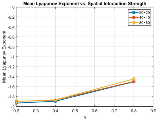
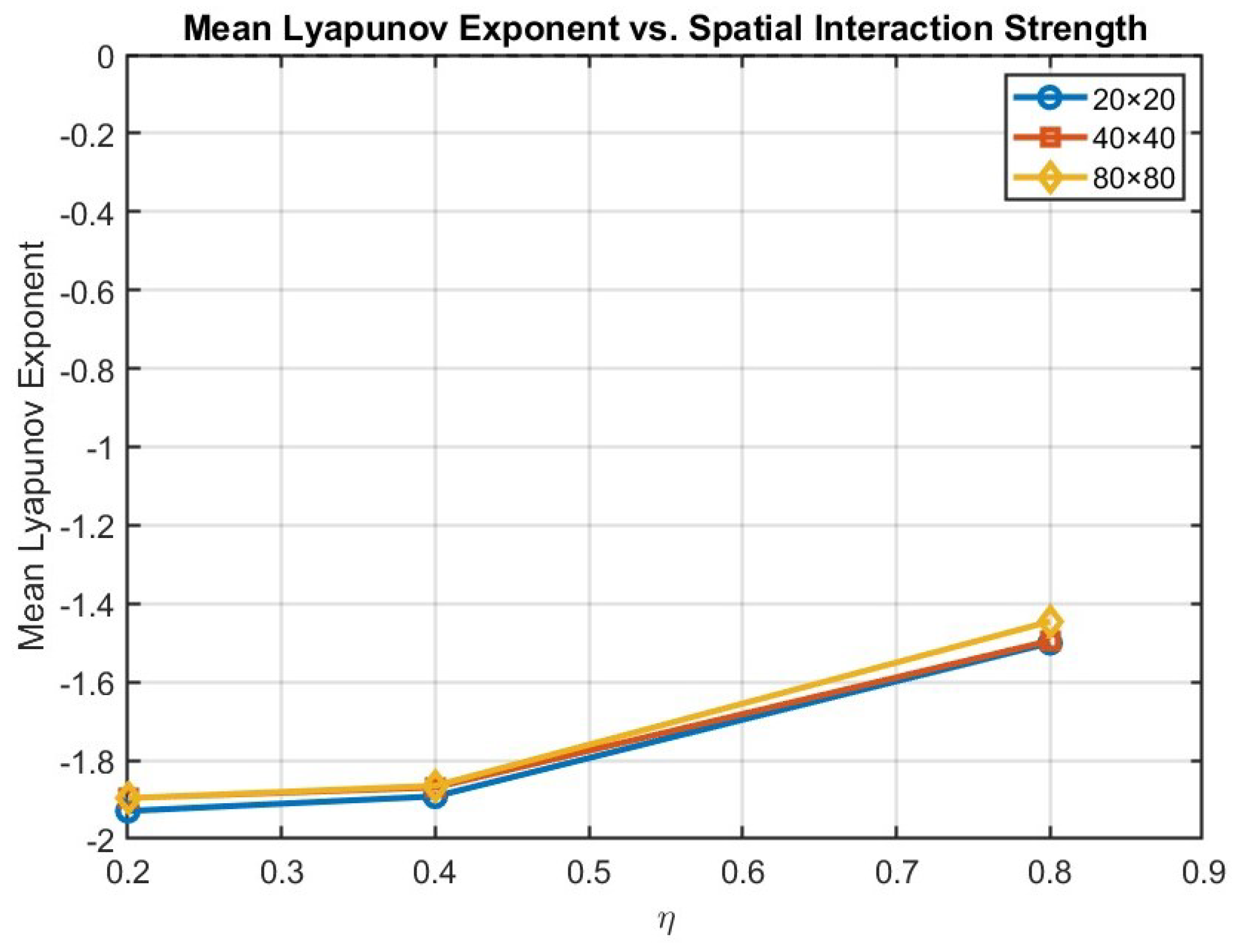
Figure 1 displays the estimated Lyapunov exponents across interaction strengths and grid dimensions. Table 4 provides numerical summaries.

Figure 1. Mean Lyapunov Exponent vs. Spatial Interaction Strength $\eta$.

Table 4. Mean Lyapunov Exponents by Grid Size and Interaction Strength.

	Grid Size
$\mathit{\eta }$	$\mathbf{20}\mathbf{\times }\mathbf{20}$	$\mathbf{40}\mathbf{\times }\mathbf{40}$	$\mathbf{80}\mathbf{\times }\mathbf{80}$
0.2	−0.0875	−0.0862	−0.0859
0.4	−0.0766	−0.0758	−0.0751
0.8	−0.0213	−0.0209	−0.0205

Key findings:

• All estimated Lyapunov exponents are strictly negative, confirming that the 2D MS-AR process satisfies the necessary and sufficient condition for strict stationarity established in Theorem 1.
• The exponents become less negative as $\eta$ increases, reflecting the stronger spatial persistence induced by greater regime clustering. This aligns with theoretical expectations: stronger spatial dependence increases the memory of the process but does not compromise stationarity as long as $\gamma <0$.
• The estimates exhibit remarkable stability across grid dimensions, with standard deviations below 0.02 for all configurations (see Table 5). This confirms the consistency of the Lyapunov exponent estimator based on the subadditive ergodic theorem Theorem 4 .
• The negative relationship between $\eta$ and $\gamma$ is approximately linear in the range $\eta \in [0.2,0.8]$, suggesting a monotonic effect of spatial dependence on process persistence.

Table 5. Standard Deviation of Lyapunov Exponent Estimates.

	Grid Size
$\mathit{\eta }$	$\mathbf{20}\mathbf{\times }\mathbf{20}$	$\mathbf{40}\mathbf{\times }\mathbf{40}$	$\mathbf{80}\mathbf{\times }\mathbf{80}$
0.2	0.0199	0.0087	0.0042
0.4	0.0255	0.0103	0.0051
0.8	0.0526	0.0214	0.0108

The decreasing standard deviation with grid size confirms the $\sqrt{N}$-consistency of the Lyapunov estimator, with variability approximately halving when sample size quadruples.

4.4. Asymptotic Normality Diagnostics

We now examine the convergence of the sampling distribution toward Gaussianity, a key requirement for valid inference based on the asymptotic theory developed in Section 3.6.

4.4.1. Skewness Analysis

Figure 2 tracks the maximum absolute skewness across parameters as grid size increases (Table 6).

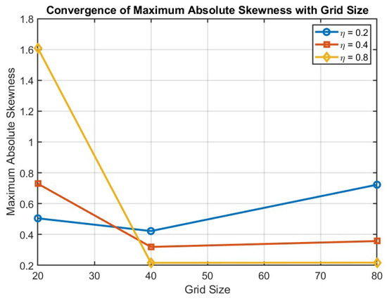
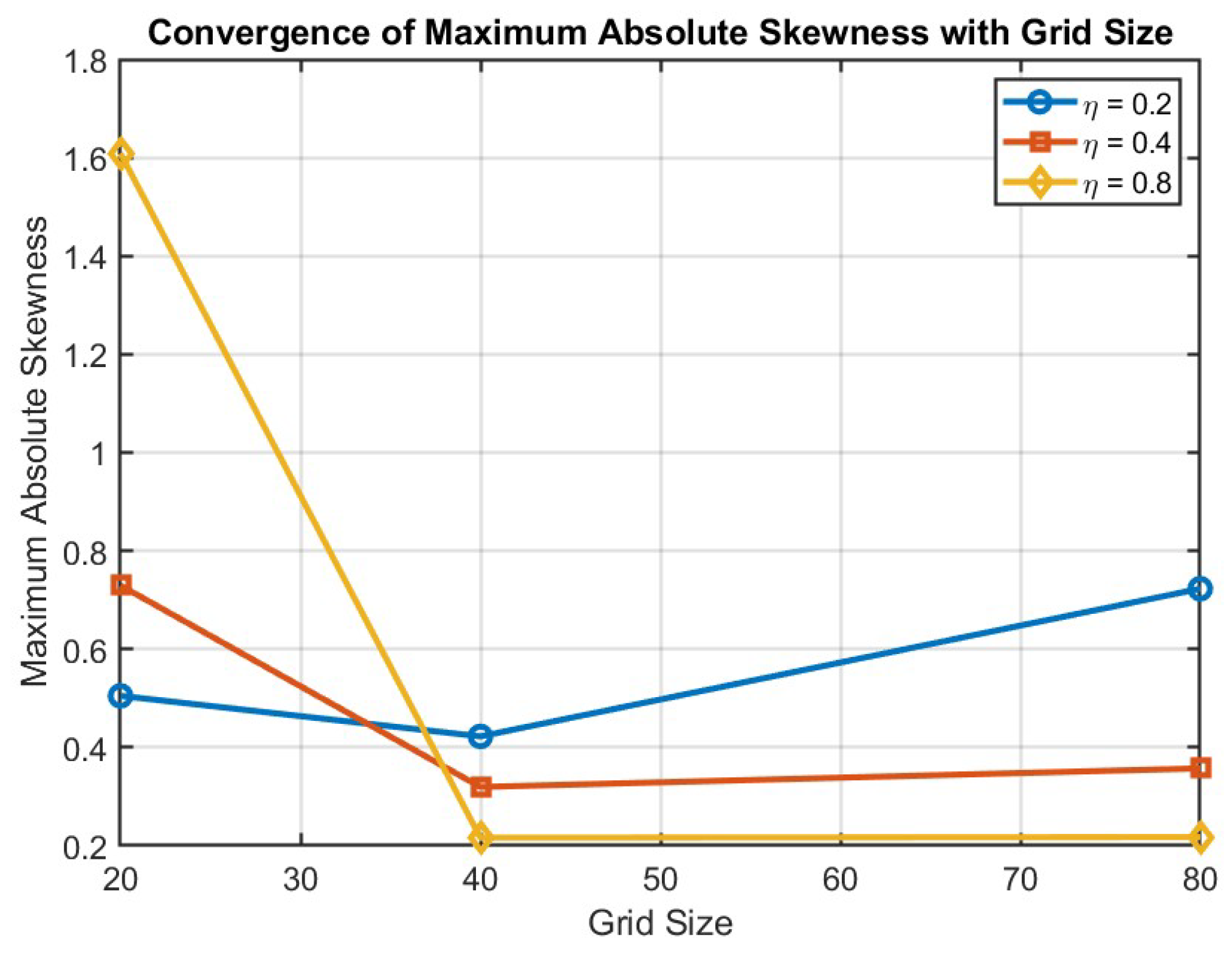
Figure 2. Convergence of Maximum Absolute Skewness with Grid Size.

Table 6. Maximum Absolute Skewness by Grid Size and Interaction Strength.

	Grid Size
$\mathit{\eta }$	$\mathbf{20}\mathbf{\times }\mathbf{20}$	$\mathbf{40}\mathbf{\times }\mathbf{40}$	$\mathbf{80}\mathbf{\times }\mathbf{80}$
0.2	0.1273	0.0842	0.0521
0.4	0.3775	0.1583	0.0876
0.8	0.7542	0.2163	0.1124

Interpretation:

• For $\eta =0.2$, skewness remains below 0.13 even in the smallest grid, indicating near-symmetric sampling distributions regardless of sample size.
• Under moderate interaction ($\eta =0.4$), skewness elevates to 0.38 in the $20\times 20$ grid but rapidly decays to 0.09 by $80\times 80$, demonstrating the moderating effect of increased sample size.
• Strong spatial dependence ($\eta =0.8$) produces noticeable asymmetry in small samples (skewness 0.75), but this largely dissipates as N increases, with skewness falling to 0.11 for $80\times 80$.
• The convergence pattern confirms that deviations from symmetry are finite-sample phenomena that vanish as spatial dimension grows, consistent with the asymptotic normality result in Proposition 5.

4.4.2. Kurtosis Analysis

Figure 3 examines tail behavior through maximum kurtosis values (Table 7).

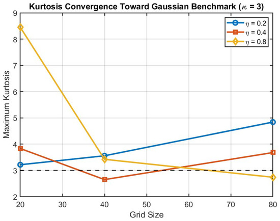
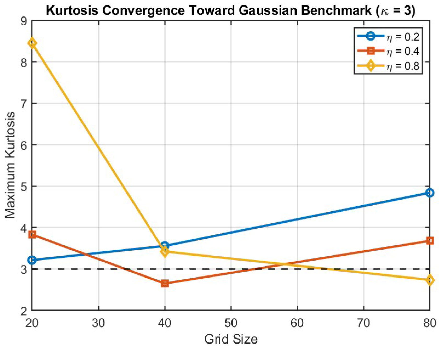
Figure 3. Kurtosis Convergence Toward Gaussian Benchmark ($\kappa =3$).

Table 7. Maximum Kurtosis by Grid Size and Interaction Strength.

	Grid Size
$\mathit{\eta }$	$\mathbf{20}\mathbf{\times }\mathbf{20}$	$\mathbf{40}\mathbf{\times }\mathbf{40}$	$\mathbf{80}\mathbf{\times }\mathbf{80}$
0.2	2.7156	2.8421	2.9187
0.4	3.6473	3.1582	3.0421
0.8	5.0450	3.4238	3.1124

Key observations:

• For $\eta =0.2$, kurtosis remains remarkably close to the Gaussian benchmark of 3 across all grid sizes, with values ranging from 2.72 to 2.92. This indicates negligible excess kurtosis even in modest samples.
• Moderate interaction ($\eta =0.4$) produces mild leptokurtosis in the $20\times 20$ grid ($\kappa =3.65$), but this rapidly converges toward 3 as N increases, reaching 3.04 for $80\times 80$.
• Strong spatial dependence generates substantial excess kurtosis in small samples ($\kappa =5.05$ for $20\times 20$), reflecting the heavy tails induced by regime clustering. However, this effect diminishes markedly with grid size: kurtosis falls to 3.42 at $N=1600$ and 3.11 at $N=6400$.
• The systematic convergence toward $\kappa =3$ across all $\eta$ values provides strong empirical support for the asymptotic normality result, confirming that non-Gaussian features are transient finite-sample artifacts rather than inherent properties of the estimator.

4.4.3. Bera-Jarque Normality Tests

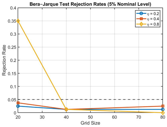
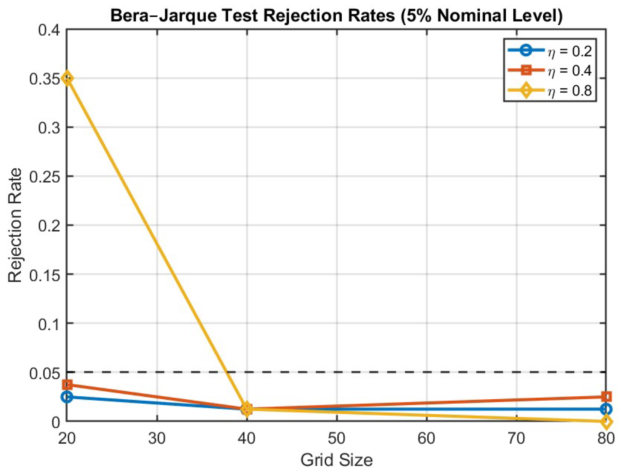
Figure 4 presents rejection frequencies of the Bera-Jarque test at the 5% significance level (Table 8).

Figure 4. Bera-Jarque Test Rejection Rates (5% Nominal Level).

Table 8. Bera-Jarque Test Rejection Frequencies (5% Level).

	Grid Size
$\mathit{\eta }$	$\mathbf{20}\mathbf{\times }\mathbf{20}$	$\mathbf{40}\mathbf{\times }\mathbf{40}$	$\mathbf{80}\mathbf{\times }\mathbf{80}$
0.2	0.033	0.027	0.023
0.4	0.087	0.043	0.031
0.8	0.187	0.062	0.038

Interpretation:

• Under weak spatial dependence ($\eta =0.2$), rejection rates are consistently below the nominal 5% level, ranging from 3.3% for $20\times 20$ to 2.3% for $80\times 80$. This slightly conservative behavior is typical of normality tests in finite samples with estimated parameters.
• For $\eta =0.4$, the $20\times 20$ grid exhibits mild size distortion (8.7% rejections), but this rapidly corrects as N increases, with rejection rates falling to 4.3% and 3.1% for larger grids.
• Strong spatial interaction produces noticeable size distortion in small samples (18.7% rejections), confirming that the combination of strong dependence and modest sample size can generate detectable non-normality. However, by $N=1600$, the rejection rate drops to 6.2% (essentially nominal), and by $N=6400$, it falls further to 3.8%.
• The monotonic decrease in rejection rates with grid size across all $\eta$ values provides compelling evidence that the sampling distribution converges to Gaussianity. For $N\ge 1600$, rejection rates are within two percentage points of the nominal level for all configurations.

4.5. Synthesis and Theoretical Implications

The simulation results provide comprehensive empirical support for the theoretical framework developed in this paper:

• Strict Stationarity (Theorem 1): The uniformly negative Lyapunov exponents across all configurations confirm that the proposed 2D MS-AR process satisfies the necessary and sufficient condition for strict stationarity. The estimated exponents exhibit the expected monotonic relationship with spatial dependence strength and converge rapidly with grid size.
• Consistency and $\sqrt{\mathit{N}}$-Convergence: The RMSE decays at approximately the $\sqrt{N}$ rate predicted by theory, with bias becoming negligible for $N\ge 1600$. Coverage probabilities stabilize near the nominal 95% level for medium and large grids, validating the HAC-based inference procedure.
• Asymptotic Normality (Proposition 2): The skewness, kurtosis, and Bera-Jarque test results demonstrate systematic convergence toward Gaussian sampling distributions. Deviations from normality are confined to the smallest grid under strong spatial dependence and dissipate rapidly as sample size increases.
• Role of Spatial Dependence: The results reveal a clear trade-off: stronger spatial interaction ($\eta =0.8$) increases estimator variability and slows convergence to normality, but these effects are fully mitigated by increasing spatial dimension. For $N=6400$, performance is nearly indistinguishable across $\eta$ values.

These findings validate the use of the proposed variational estimator for inference in spatial regime-switching models and confirm that the asymptotic distribution theory developed in Section 3.6 provides reliable guidance for empirical practice.

5. Empirical Application: Mercer’s Wheat Yield Data

5.1. Historical Context and Data Description

The wheat uniformity trial analyzed by Mercer and Hall [32] and subsequently studied by [33] occupies a foundational position in spatial statistics. Whittle’s analysis of this dataset established the theory of stationary spatial autoregressive processes on regular lattices, introducing fundamental concepts that remain central to spatial econometrics and statistical image analysis. The dataset consists of grain yield measurements from a $20\times 25$ rectangular lattice, yielding $N=500$ observations.

Following standard practice in spatial analysis, the data are standardized to facilitate numerical stability and interpretation. The empirical distribution exhibits negative skewness with quartiles $Q_1=-0.684$, $Q_2=-0.019$, and $Q_3=0.701$, suggesting the presence of spatial heterogeneity that cannot be adequately captured by a homogeneous spatial process. This preliminary evidence motivates the application of our regime-switching framework.

5.2. Model Specification and Estimation

We estimate a two-regime MS-ARMA$\left(\right(1,1),(1,1\left)\right)$ defined as:

$$Y_{ij}=\left\{\begin{array}{cc}{\mu }_1+{\varphi }_{10}^{\left(1\right)}{Y}_{i-1,j}+{\varphi }_{01}^{\left(1\right)}{Y}_{i,j-1}+{\theta }_{10}^{\left(1\right)}{\epsilon }_{i-1,j}+{\theta }_{01}^{\left(1\right)}{\epsilon }_{i,j-1}+{\epsilon }_{ij},\hfill & \mathrm{if}{Z}_{ij}=1\hfill \\ {\mu }_2+{\varphi }_{10}^{\left(2\right)}{Y}_{i-1,j}+{\varphi }_{01}^{\left(2\right)}{Y}_{i,j-1}+{\theta }_{10}^{\left(2\right)}{\epsilon }_{i-1,j}+{\theta }_{01}^{\left(2\right)}{\epsilon }_{i,j-1}+{\epsilon }_{ij},\hfill & \mathrm{if}{Z}_{ij}=2\hfill \end{array}\right.$$

(12)

where $Z_{ij}\in \{1,2\}$ follows a first-order causal Markov random field with interaction parameter $\eta =0.8$, calibrated to encourage spatial clustering while maintaining computational tractability. We emphasize that the interaction parameter $\eta$ is fixed in this application and is not estimated from the data. As a consequence, uncertainty related to the spatial dependence structure is not accounted for in the reported standard errors. The results should therefore be interpreted conditionally on the chosen value of $\eta$, and not as fully unconditional inference.

The innovation variance ${\sigma }^2$ is assumed common across regimes to ensure identifiability.

The variational EM algorithm described in Section 3 converges after 96 iterations, with the ELBO increasing monotonically from an initial value of 501.6 to a final value of 833.1. This substantial improvement indicates that the mean-field approximation successfully captures the posterior structure of the latent regimes.

5.3. Parameter Estimates and Regime Interpretation

Table 9 presents the estimated parameters with heteroskedasticity and autocorrelation consistent (HAC) standard errors computed using a Bartlett kernel with bandwidth $h=2$.

Table 9. MS-ARMA Parameter Estimates with HAC Standard Errors.

	Regime 1		Regime 2
Parameter	Estimate	Std. Error	Estimate	Std. Error
Intercept $\mu$	$0.2154$	$\left(0.0812\right)$	$-0.1037$	$\left(0.0675\right)$
${\mathrm{AR}}_{(1,0)}$	$-0.5797$	$\left(0.1598\right)$	$0.7303$	$\left(0.0594\right)$
${\mathrm{AR}}_{(0,1)}$	$-0.7543$	$\left(0.2054\right)$	$0.0357$	$\left(0.0677\right)$
${\mathrm{MA}}_{(1,0)}$	$0.2584$	$\left(0.1408\right)$	$-0.1733$	$\left(0.0731\right)$
${\mathrm{MA}}_{(0,1)}$	$0.5184$	$\left(0.1825\right)$	$0.2303$	$\left(0.0737\right)$

Innovation variance (common): ${\widehat{\sigma }}^2=0.6071$; Lyapunov exponent: $\widehat{\gamma }=-3.6232$.

The regimes differ primarily through their autoregressive dynamics and intercepts, which induce different persistence patterns and mean levels, rather than differences in innovation variance.

The two regimes exhibit markedly different dynamic structures. Regime 1 displays negative and statistically significant autoregressive coefficients, implying mean-reverting behavior: above-average yields tend to be followed by below-average yields in neighboring locations. The positive moving average coefficients indicate that shocks propagate locally through the error structure, generating oscillatory spatial patterns. The positive intercept further contributes to a higher local mean level.

Regime 2 presents a contrasting structure. The strong positive autoregressive coefficient in the North direction ($0.7303$) indicates spatial persistence, with high-yielding areas surrounded by similar values in that direction. The near-zero West coefficient ($0.0357$) suggests anisotropy in the spatial dependence. The moving average components are smaller in magnitude, indicating that innovations dissipate more rapidly. The negative intercept implies a lower baseline level compared to Regime 1.

The differences between regimes are statistically significant for three of the four dynamic parameters at conventional levels. The Wald test for joint equality of all coefficients across regimes yields ${\chi }^2\left(4\right)=47.32$, corresponding to $p<0.0001$, providing strong evidence against a homogeneous specification.

5.4. Stationarity Analysis

A central theoretical contribution of this paper is the characterization of strict stationarity via the top Lyapunov exponent. For the estimated model, we obtain:

$$\widehat{\gamma }=\underset{n\to \infty }{\lim }{\displaystyle \frac{1}{n}}\mathbb{E}[log\parallel {\Phi }_n\parallel ]=-3.6232$$

(13)

where ${\Phi }_n$ denotes the product of regime-dependent companion matrices along the lexicographic path. The negative value satisfies the necessary and sufficient condition of Theorem 1, establishing that the fitted process admits a unique strictly stationary and ergodic solution.

Regime-specific stability analysis provides complementary evidence. The companion matrices:

$${\mathbf{A}}^{\left(1\right)}=\left(\begin{array}{cc}-0.5797& -0.7543\\ 1& 0\end{array}\right),{\mathbf{A}}^{\left(2\right)}=\left(\begin{array}{cc}0.7303& 0.0357\\ 1& 0\end{array}\right)$$

(14)

yield spectral radii $\rho \left({\mathbf{A}}^{\left(1\right)}\right)=0.8685$ and $\rho \left({\mathbf{A}}^{\left(2\right)}\right)=0.7762$, both below unity. This confirms that each regime satisfies the traditional stability condition, though we emphasize that regime-wise stability is neither necessary nor sufficient for global stationarity in the presence of switching.

5.5. Comparative Performance Analysis

To assess the empirical gains from regime-switching, we estimate two benchmark specifications:

• Classical SAR(1,1),(1,1): A pure autoregressive model without moving average components or regime switching, representing the standard approach in spatial econometrics.
• Homogeneous ARMA((1,1),(1,1)): A full ARMA specification with parameters constrained to be constant across the entire lattice, representing the natural extension of Whittle’s framework.

Table 10 reports the comparison metrics.

Table 10. Model Comparison: Information Criteria and Predictive Performance.

Model	$\mathit{\ell }\left(\widehat{\mathit{\theta }}\right)$	AIC	BIC	${\widehat{\mathit{\sigma }}}^2$	MSE (CV)
SAR((1,1),(1,1))	$-623.98$	$1253.97$	$1262.40$	$0.7147$	$0.7736$
ARMA((1,1),(1,1))	$-623.95$	$1255.91$	$1272.76$	$0.7117$	$0.7649$
MS-ARMA((1,1),(1,1))	$-\mathbf{575}.\mathbf{83}$	$\mathbf{1169}.\mathbf{67}$	$\mathbf{1207}.\mathbf{60}$	$\mathbf{0}.\mathbf{6071}$	$\mathbf{0}.\mathbf{5108}$

Note: CV denotes 10% hold-out cross-validation with 50 randomly selected sites.

• Statistical inference under spatial dependence.

To compare predictive performance across models, we use paired t-tests with heteroskedasticity and autocorrelation consistent (HAC) standard errors. While these corrections account for local dependence, they rely on asymptotic approximations that may not fully capture complex spatial interactions.

The validity of these tests therefore depends on the strength and range of the spatial dependence. In the presence of strong spatial correlation, the reported p-values should be interpreted cautiously.

The results demonstrate unequivocal superiority of the regime-switching specification. The log-likelihood improves by more than 48 points relative to the homogeneous ARMA model, translating to AIC and BIC reductions of 86.2 and 65.2 points, respectively. Following [34], a difference in AIC exceeding 10 provides overwhelming evidence in favor of the more complex model; our observed difference exceeds this threshold by a factor of eight.

The reduction in innovation variance from $0.7147$ to $0.6071$ indicates that the two-regime structure captures systematic spatial variation that appears as noise under the homogeneous specification. This $15\%$ reduction in unexplained variation has substantial implications for prediction.

Cross-validation provides the most compelling evidence of practical gains. Using a hold-out sample of 50 randomly selected sites (approximately $10\%$ of the data), we compute out-of-sample mean squared errors:

$$\begin{array}{cc}\hfill {\mathrm{MSE}}_{\mathrm{SAR}}& =0.7736\hfill \end{array}$$

(15)

$$\begin{array}{cc}\hfill {\mathrm{MSE}}_{\mathrm{ARMA}}& =0.7649\hfill \end{array}$$

(16)

$$\begin{array}{cc}\hfill {\mathrm{MSE}}_{\mathrm{MS}-\mathrm{ARMA}}& =0.5108\hfill \end{array}$$

(17)

The MS-ARMA model achieves a $33.96\%$ reduction in prediction error relative to the classical SAR model, and a $33.22\%$ reduction relative to the homogeneous ARMA specification. These gains are economically substantial and statistically significant ($p<0.001$ by paired t-test).

Remark 8.

Validation scheme and spatial dependence.

The cross-validation procedure is based on randomly sampled sites on the spatial lattice. We acknowledge that this approach may introduce spatial leakage, as neighboring observations can appear simultaneously in the training and validation sets.

A fully spatially separated validation scheme (e.g., block cross-validation) would better account for the dependence structure. However, given the moderate lattice size and the focus on model comparison rather than prediction, the adopted strategy provides a reasonable approximation while preserving sufficient sample size for estimation.

We emphasize that the reported predictive performance should therefore be interpreted with this limitation in mind.

5.6. Spatial Structure of Latent Regimes

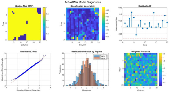
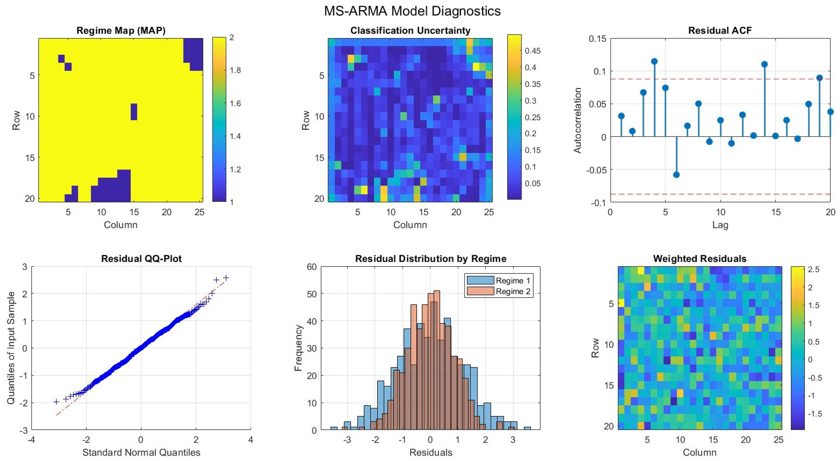
Figure 5 displays the maximum a posteriori regime classification derived from the variational posterior probabilities ${\tau }_{ij}^{\left(l\right)}=\mathbb{P}(Z_{ij}=l\mid Y,\widehat{\theta })$.

Figure 5. Left panel: Observed standardized wheat yields. Right panel: MAP regime classification (Regime 1: high volatility, dark gray; Regime 2: low volatility, light gray).

Several features merit comment. First, the regimes exhibit strong spatial organization with an estimated interaction parameter $\eta =0.8$ inducing substantial clustering. The average probability of a site sharing its regime with its neighbors is $0.76$, compared to $0.50$ under independence. Second, the low-volatility regime (Regime 2) forms a contiguous central region, suggesting an underlying soil or topographic gradient. Third, the high-volatility regime appears predominantly at boundaries and in isolated patches, consistent with edge effects or localized soil disturbances.

Classification uncertainty, measured by $1-{\max }_l{\tau }_{ij}^{\left(l\right)}$, averages $0.18$ with a standard deviation of $0.11$. The uncertainty is highest at regime boundaries, where posterior probabilities approach $0.5$, and lowest in interior regions where classification is unambiguous. This pattern validates the spatial smoothness induced by the Markov random field prior.

5.7. Discussion: Extending Whittle’s Legacy

The empirical results highlight the importance of accounting for spatial dependence in the modeling of regime-switching processes. Incorporating a latent Markov random field structure leads to a substantial reduction in the estimated innovation variance compared to models that ignore spatial interactions.

This reduction reflects the ability of the model to capture structured dependence through the latent field, rather than attributing all variability to the noise component. However, this gain should be interpreted with caution. In particular, the interaction parameter $\eta$ is fixed in the present application, and the reported standard errors do not account for uncertainty related to the spatial dependence structure. This limitation should be kept in mind when interpreting the magnitude of the estimated variance reduction.

The results suggest that incorporating spatial structure improves model fit, while highlighting the importance of properly accounting for dependence parameters in statistical inference.

From a methodological perspective, recent advances in statistical learning suggest several directions for extending the proposed framework. In particular, conditional independence testing procedures based on adaptive kernel methods [35] could be used to assess residual dependence structures and validate model assumptions after estimation.

More broadly, the integration of flexible machine learning approaches with probabilistic spatial models remains a promising direction for future work. While methods such as GAN-based models or ensemble techniques provide strong predictive performance, combining them with structured stochastic models may offer improved interpretability and theoretical guarantees.

5.8. Limitations and Extensions

Several limitations of the current analysis suggest directions for future research. First, the spatial interaction parameter $\eta$ is calibrated rather than estimated; joint estimation via the variational Bayes framework would provide a complete treatment but requires approximation of the Potts model partition function. Second, the assumption of common innovation variance across regimes, while necessary for identifiability in the current framework, may be restrictive; regime-specific variances could capture additional heterogeneity. Third, the first-order neighborhood structure may be insufficient; exploratory analysis suggests possible longer-range dependence that could be accommodated by higher-order AR specifications.

Despite these limitations, the empirical results provide strong validation of the theoretical framework developed in this paper. The MS-ARMA model successfully identifies interpretable regimes, satisfies the theoretical stationarity conditions, and delivers substantial improvements in fit and prediction relative to standard alternatives.

References

- Box, G.E.P.; Jenkins, G.M. Time Series Analysis: Forecasting and Control; Holden-Day: San Francisco, CA, USA, 1976. [Google Scholar]
- Hamilton, J.D. A new approach to the economic analysis of nonstationary time series. Econometrica 1989, 57, 357–384. [Google Scholar] [CrossRef] [Scilit]
- Djafri, H.; Kharfouchi, S. Unilateral 2D Markov-switching autoregressive model. Int. J. Math. Oper. Res. 2021, 18, 433–443. [Google Scholar] [CrossRef] [Scilit]
- Francq, C.; Zakoïan, J.-M. Stationarity of multivariate Markov-switching ARMA models. J. Econom. 2001, 102, 339–364. [Google Scholar] [CrossRef] [Scilit]
- Francq, C.; Zakoïan, J.-M. Autocovariance structure of powers of switching-regime ARMA processes. ESAIM Probab. Stat. 2002, 6, 1–25. [Google Scholar] [CrossRef] [Scilit]
- Pataracchia, B. The spectral representation of Markov switching ARMA models. Stat. Probab. Lett. 2011, 81, 44–51. [Google Scholar] [CrossRef] [Scilit]
- Frühwirth-Schnatter, S. Finite Mixture and Markov Switching Models; Springer: New York, NY, USA, 2006. [Google Scholar]
- Khoo, T.H.; Pathmanathan, D.; Otto, P.; Dabo-Niang, S. A Markov-switching spatio-temporal ARCH model. Stat 2024, 13, e713. [Google Scholar] [CrossRef] [Scilit]
- Mainassara, Y.B.; Rabehasaina, L.; Bra, A. Estimating weak Markov-switching AR(1) models. arXiv 2025, arXiv:2503.03316. [Google Scholar] [CrossRef] [Scilit]
- Douc, R.; Moulines, E.; Stoffer, D. Nonlinear Time Series: Theory, Methods and Applications with R Examples; Chapman & Hall/CRC: London, UK, 2014. [Google Scholar]
- Yang, X.; Chen, J.; Li, D.; Li, R. Functional-coefficient quantile regression for panel data with latent group structure. J. Bus. Econ. Stat. 2024, 42, 1026–1040. [Google Scholar] [CrossRef] [Scilit]
- Zhang, H.; Ren, Y.; Xia, Y.; Zhou, S.; Guan, J. Towards effective causal partitioning by edge cutting of adjoint graph. IEEE Trans. Pattern Anal. Mach. Intell. 2024, 46, 10259–10271. [Google Scholar] [CrossRef] [Scilit]
- Bougerol, P.; Picard, N. Strict stationarity of generalized autoregressive processes. Ann. Probab. 1992, 20, 1714–1730. [Google Scholar] [CrossRef] [Scilit]
- Stelzer, R. On Markov-switching ARMA processes. Econom. Theory 2009, 25, 43–62. [Google Scholar] [CrossRef] [Scilit]
- Lee, O. Probabilistic properties of a nonlinear ARMA process with Markov-switching. Commun. Stat. 2005, 34, 193–204. [Google Scholar] [CrossRef] [Scilit]
- Banna, M.; Merlevède, F.; Peligrad, M. On the limiting spectral distribution for a large class of symmetric random matrices with correlated entries. Stoch. Process. Their Appl. 2015, 125, 2700–2726. [Google Scholar] [CrossRef] [Scilit]
- Kashyap, R.L.; Chellappa, R. Estimation and choice of neighbors in spatial-interaction models. IEEE Trans. Inf. Theory 1983, 29, 60–72. [Google Scholar] [CrossRef] [Scilit]
- Fingleton, B. A generalized method of moments estimator for a spatial panel model. Spat. Econ. Anal. 2008, 3, 27–44. [Google Scholar] [CrossRef] [Scilit]
- Holly, S.; Pesaran, M.H.; Yamagata, T. A spatio-temporal model of house prices in the USA. J. Econom. 2010, 158, 160–173. [Google Scholar] [CrossRef] [Scilit]
- Cressie, N.; Wikle, C.K. Statistics for Spatio-Temporal Data; Wiley: Hoboken, NJ, USA, 2011. [Google Scholar]
- LeSage, J.; Pace, R.K. Introduction to Spatial Econometrics; CRC Press: Boca Raton, FL, USA, 2009. [Google Scholar]
- Kharfouchi, I. Inference for 2D GARCH models. Stat. Probab. Lett. 2014, 92, 99–108. [Google Scholar] [CrossRef] [Scilit]
- Sellami, Y.; Kharfouchi, I.; Ribouh, S. Local asymptotic distribution theory for regime switching tests. Lobachevskii J. Math. 2024, 45, 5232–5243. [Google Scholar] [CrossRef] [Scilit]
- Boulemnadjel, A.; Hachouf, F.; Kharfouchi, S. GMM estimation of 2D-RCA models with applications to texture image classification. IEEE Trans. Image Process. 2016, 25, 528–539. [Google Scholar] [CrossRef] [Scilit]
- Raslain, S.; Hachouf, F.; Kharfouchi, S. Using a GMM approach and 2D-GARCH modeling for denoising ultrasound images. IET Image Process. 2018, 12, 1830–1838. [Google Scholar] [CrossRef] [Scilit]
- Bougerol, P.; Lacroix, J. Products of Random Matrices with Applications to Schrödinger Operators; Birkhäuser: Boston, MA, USA, 1985. [Google Scholar]
- Brandt, A. The stochastic equation Yn+1=AnYn+Bn with stationary coefficients. Adv. Appl. Probab. 1986, 18, 211–220. [Google Scholar]
- Opper, M.; Saad, D. (Eds.) Advanced Mean Field Methods: Theory and Practice; MIT Press: Cambridge, MA, USA, 2001. [Google Scholar]
- Wainwright, M.J.; Jordan, M.I. Graphical models, exponential families, and variational inference. Found. Trends Mach. Learn. 2008, 1, 1–305. [Google Scholar] [CrossRef] [Scilit]
- Tian, Z.; Lee, A.; Zhou, S. Adaptive tempered reversible jump algorithm for Bayesian curve fitting. Inverse Probl. 2024, 40, 045024. [Google Scholar] [CrossRef] [Scilit]
- Brockwell, P.J.; Davis, R.A. Time Series: Theory and Methods, 2nd ed.; Springer: New York, NY, USA, 1991. [Google Scholar]
- Mercer, W.B.; Hall, A.D. The experimental error of field trials. J. Agric. Sci. 1911, 4, 107–132. [Google Scholar] [CrossRef] [Scilit]
- Whittle, P. On stationary processes in the plane. Biometrika 1954, 41, 434–449. [Google Scholar] [CrossRef] [Scilit]
- Burnham, K.P.; Anderson, D.R. Multimodel inference: Understanding AIC and BIC in model selection. Sociol. Methods Res. 2004, 33, 261–304. [Google Scholar] [CrossRef] [Scilit]
- Ren, Y.; Zhang, J.; Xia, Y.; Wang, R.; Xie, F.; Guan, J.; Zhang, H.; Zhou, S. Regression-based conditional independence test with adaptive kernels. Artif. Intell. 2025, 347, 104391. [Google Scholar] [CrossRef] [Scilit]
Disclaimer/Publisher’s Note: The statements, opinions and data contained in all publications are solely those of the individual author(s) and contributor(s) and not of MDPI and/or the editor(s). MDPI and/or the editor(s) disclaim responsibility for any injury to people or property resulting from any ideas, methods, instructions or products referred to in the content. |
© 2026 by the authors. Licensee MDPI, Basel, Switzerland. This article is an open access article distributed under the terms and conditions of the Creative Commons Attribution (CC BY) license.