Odd Right-End Numerical Semigroups

Abstract

An odd right-end semigroup (hereinafter Ore semigroup) is a numerical semigroup S verifying that $x+1\in S$ for every $x\in S\setminus \left\{0\right\}$ such that x is even. The introduction and study of these semigroups is the purpose of the present work. In particular, we will give some algorithms which compute all Ore semigroups with a given genus, a fixed Frobenius number and a specific multiplicity. We will see that if X is a set of positive integers, then there exists the smallest Ore semigroup, under the inclusion sets, that contains X. We will denote this semigroup by $\theta \left[X\right]$ and present an algorithm to calculate it. Finally, we will study the embedding dimension, the Frobenius number, and the genus of Ore semigroups of the form $\theta \left[\right\{m\left\}\right]$, where m is a positive integer. As a consequence of this study, we will prove that this kind of semigroup satisfies Wilf’s conjecture.

1. Introduction

Consider $\mathbb{Z}$ a set of integers and let $\mathbb{N}$ be the set of non-negative integers. A subset S of $\mathbb{N}$ containing 0 is a submonoid of $(\mathbb{N},+)$ if it is closed under the addition. A submonoid S of $(\mathbb{N},+)$ is a numerical semigroup if $\mathbb{N}\setminus S=\{x\in \mathbb{N}\mid x\notin S\}$ is a finite set.

Given a numerical semigroup S there exist three very important elements: the multiplicity, the Frobenius number and the genus, defined by $\mathrm{m}\left(S\right)=\min (S\setminus \{0\},$ $\mathrm{F}\left(S\right)=\max \{z\in \mathbb{Z}\mid z\notin S\}$ and $\mathrm{g}\left(S\right)=♯(\mathbb{N}\setminus S)$ (where $♯X$ denotes the cardinality of a set X), respectively.

Let A be a non-empty subset of $\mathbb{N}.$ Denote by $⟨A⟩$ the submonoid of $(\mathbb{N},+)$ generated by A. That is,

$$⟨A⟩=\{{\alpha }_1{a}_1+\dots +{\alpha }_r{a}_r\mid r\in \mathbb{N}\setminus \left\{0\right\},\{a_1, \dots , a_r\}\subseteq A \mathrm{and} \{{\alpha }_1, \dots , {\alpha }_r\}\subseteq \mathbb{N}\}.$$

It is verified that $⟨A⟩$ is a numerical semigroup if and only if $\gcd \left(A\right)=1$ (see ([1] Lemma 2.1)).

Suppose A is a non-empty subset of $\mathbb{N}$ and M is a submonoid of $(\mathbb{N},+).$ If $M=⟨A⟩,$ then A is called a system of generators of $M.$ In addition, A will be called a minimal system of generators of M if $M\ne ⟨B⟩$ for all $B⊊A.$ It is verified that every submonoid of $(\mathbb{N},+)$ has a unique minimal system of generators, which, in addition, is finite (see ([1] Corollary 2.8)). The minimal system of generators of a submonoid M is denoted by $\mathrm{msg}\left(M\right).$ We will call the cardinality of $\mathrm{msg}\left(M\right)$ the embedding dimension of $M$, denoted by $\mathrm{e}\left(M\right).$

In the study of numerical semigroups, the Frobenius problem (see [2]) involves finding explicit formulas to determine both the Frobenius number and the genus based on its minimal system of generators. While Sylvester [3] provided a solution for semigroups with embedding dimension two, the problem remains an open challenge for those numerical semigroups with embedding dimension three or higher. Nevertheless, specific solutions have been extensively documented for various subfamilies of numerical semigroups (see, for example, [4,5,6,7,8,9]).

Another important unresolved issue in the theory of numerical semigroups concerns the relationship between the Frobenius number, genus, and embedding dimension. This is summarized in Wilf’s conjecture (see [10]), given that $\mathrm{e}\left(S\right)\mathrm{g}\left(S\right)\le \left(\mathrm{e}\right(S)-1)\left(\mathrm{F}\right(S)+1).$ Despite being one of the most important challenges in the discipline, this conjecture has only been proven for particular classes of semigroups, as documented in the works of [11,12,13,14,15], among others.

For each $g\in \mathbb{N},$ the set $\mathrm{S}\left(g\right)=\{S\mid S \text{is a numerical semigroup and} \mathrm{g}(S)=g\}$ has been extensively studied in the literature (see [16,17,18,19,20]), often motivated by the conjecture introduced in [18]. This conjecture posits that the sequence of cardinalities ${\{\#\mathrm{S}\left(g\right)\}}_{g\in \mathbb{N}}$ is increasing and behaves similarly to the Fibonacci sequence. While Zhai ([21]) established that ${\displaystyle \underset{g\to \infty }{\lim }\frac{\#\mathrm{S}\left(g\right)}{\#\mathrm{S}(g-1)}}$ is the golden number and therefore the asymptotic behavior of the sequence ${\{\#\mathrm{S}\left(g\right)\}}_{g\in \mathbb{N}}$ is similar to the behavior of the Fibonacci sequence. Nevertheless, whether $\#\mathrm{S}(g-1)\le \#\mathrm{S}\left(g\right)$ for every $g\in \mathbb{N}\setminus \left\{0\right\},$ is still unresolved to this day.

An odd right-end numerical semigroup (hereinafter Ore semigroup) is a numerical semigroup S verifying that $x+1\in S$ for every $x\in S\setminus \left\{0\right\}$ such that x is even. The main goal of this paper is to study these semigroups.

Denote by $\theta =\{S\mid S \text{is an Ore semigroup}\}.$ In Section 2, we first establish that $\theta$ is a Frobenius variety. This fact, together the results from [22], will allow us to construct a tree whose vertices are the set $\theta .$ In Section 3, as an application of the above tree structure, we develop algorithmic procedure to determine all Ore semigroups with a given genus.

If $X\subseteq \mathbb{N}\setminus \left\{0\right\}$ is non-empty, in Section 4, we will see that the set defined as $\theta \left(X\right)=\{S\mid S \mathrm{is} \mathrm{an} \mathrm{Ore} \mathrm{semigroup} \mathrm{and} X\subseteq S\}$ is a Frobenius variety with finite cardinality. As a consequence, we will obtain that ${\displaystyle \theta \left[X\right]=\bigcap _{S\in \theta \left(X\right)}S}$ is the smallest Ore semigroup that contains $X.$ If $S=\theta \left[X\right],$ then we say that X is an Ore system of generators of $S.$ Additionally, if $S\ne \theta \left[Y\right]$ for all $Y⊊X,$ then X is an Ore minimal system of generators of $S.$ In Section 4 we will also see that every Ore semigroup has a unique Ore minimal system of generators. It will be denoted by $\theta \mathrm{msg}\left(S\right)$ and its cardinality is called the $\theta \mathrm{rank}$ of S, denoted by $\theta \mathrm{rank}\left(S\right).$ Section 4 will conclude by showing an algorithm that calculates $\theta \left[X\right],$ starting from a finite and non-empty subset X of $\mathbb{N}\setminus \left\{0\right\}.$

In Section 5, we will study the Ore semigroups with $\theta \mathrm{rank}$ $1.$ We will give formulas for obtaining the embedding dimension, Frobenius number, and genus. As a consequence, we will verify that this type of semigroup satisfies Wilf’s conjecture.

Section 6 is devoted to see that ${\theta }_m=\{S\mid S \text{is an Ore semigroup and} \mathrm{m}\left(S\right)=m\},$ where $m\in \mathbb{N}\setminus \{0, 1\},$ is a Frobenius pseudo-variety with finite cardinality. Combining this fact with the results of [23], we can build a tree whose vertex set is ${\theta }_m$, thus yielding an algorithm to compute all elements in ${\theta }_m$.

Lastly, we show in Section 7 that if F is a positive integer, then the set defined as $\theta \left(F\right)=\{S\mid S \mathrm{is} \mathrm{an} \mathrm{Ore} \mathrm{semigroup} \mathrm{and} \mathrm{F}(S)=F\}$ is a covariety. This fact, together with the results from [24], allows us to construct a tree whose vertex set is $\theta \left(F\right)$ and, consequently, to design an algorithm that computes all elements of $\theta \left(F\right).$

To conclude, we would like to point out that in this introduction we have presented three of the most significant problems in the theory of numerical semigroups, namely the Frobenius problem, Wilf’s conjecture and the conjecture of Bras-Amoros. In our work, we have shown how to calculate all Ore semigroups with a given genus. In this sense, we follow the line of research associated with the Bras-Amorós conjecture. We have solved the Frobenius problem for Ore semigroups of rank one and have also seen that these semigroups verify Wilf’s conjecture. Therefore, the introduction and study of Ore semigroups is sufficiently motivated and justified by their contribution to the progress and resolution of these three major problems.

2. The Tree of the Ore Semigroups

A Frobenius variety is a non-empty family of semigroups $\mathcal{V}$, which verifies the following:

1.

If $\{S, T\}\subseteq \mathcal{V},$ then $S\cap T\in \mathcal{V}.$

2.

If $S\in \mathcal{V}$ and $S\ne \mathbb{N},$ then $S\cup \left\{\mathrm{F}\right(S\left)\right\}\in \mathcal{V}.$

In this section, we first aim to show that $\theta =\{S\mid S \text{is an Ore semigroup}\}$ is a Frobenius variety. Since $\{0, m, \to \}\in \theta$ for all $m\in \mathbb{N}$ (with → indicating that all integers greater than or equal to m are included), it follows that $\theta$ is infinite.

It is evident that $\mathrm{F}\left(\mathbb{N}\right)=-1$ and $\mathrm{F}\left(S\right)\in \mathbb{N}\setminus \left\{0\right\}$ for every numerical semigroup S such that $S\ne \mathbb{N}.$

We can easily see the following result.

Lemma 1.

Given S and T numerical semigroups, the following conditions are verified.

1. 

If $S\ne \mathbb{N},$ then $S\cup \left\{\mathrm{F}\right(S\left)\right\}$ is a numerical semigroup.

2. 

$S\cap T$ is a numerical semigroup.

3. 

$\mathrm{F}(S\cap T)=\max \left\{\mathrm{F}\right(S), \mathrm{F}(T\left)\right\}.$

4. 

$\mathrm{m}(S\cap T)\ge \max \left\{\mathrm{F}\right(S), \mathrm{F}(T\left)\right\}.$

By applying Lemma 1, the following result has a simple proof.

Proposition 1.

With the above notation, θ is a Frobenius variey.

A pair $(V, E)$ where V is a non-empty set and E is a subset of $\left\{\right(u, v)\in V\times V\mid u\ne v\}$ is called a graph and it will be denoted by $G.$ The vertices and edges of G will be the element of V and and E, respectively.

A path of length n, connecting the vertices u and v of G is a sequence of different edges of the form $(v_0, v_1), (v_1, v_2), \dots , (v_{n-1}, v_n)$ such that $v_0=u$ and $v_n=v$.

A graph G is a tree if there exists a vertex r (known as the root of G) such that for any other vertex v of G there exists a unique path connecting v and r. If $(u, v)$ is an edge of the tree G, we say that u is a child of v.

Now let us consider the graph $\mathrm{G}\left(\theta \right)$ defined as follows: the set of vertices is $\theta$ and $(S, T)\in \theta \times \theta$ is an edge if and only if $T=S\cup \left\{\mathrm{F}\right(S\left)\right\}.$

By virtue of Proposition 1 and ([22] Theorem 27), we arrive at the following result.

Theorem 1.

$\mathrm{G}\left(\theta \right)$ is a rooted tree at $\mathbb{N}.$ Moreover, the set formed by the children of a vertex S of the tree $\mathrm{G}\left(\theta \right)$ is $\{S\setminus \{x\}\mid x\in \mathrm{msg}(S), x>\mathrm{F}(S) and S\setminus \{x\}\in \theta \}.$

We refer to ([1] Lemma 2.3) for the next result.

Lemma 2.

Let S be a numerical semigroup and $x\in S.$ Then $S\setminus \left\{x\right\}$ is a numerical semigroup if and only if $x\in \mathrm{msg}\left(S\right).$

The following result will allow us to easily determine the immediate descendants of an arbitrary vertex of tree $\mathrm{G}\left(\theta \right).$

Proposition 2.

Let S be an Ore semigroup and $x\in \mathrm{msg}\left(S\right)$ such that $x>\mathrm{F}\left(S\right).$ Then $S\setminus \left\{x\right\}$ is an Ore semigroup if and only if $x=\mathrm{F}\left(S\right)+1$ or x is even.

Proof. 

(Necessity). If $x\ne \mathrm{F}\left(S\right)+1,$ then $x-1\in S\setminus \left\{x\right\}.$ As $x\notin S\setminus \left\{x\right\}$ and $S\setminus \left\{x\right\}$ is an Ore semigroup, then $x-1$ is odd and x is even.

(Sufficiency). By Lemma 2, we have that $S\setminus \left\{x\right\}$ is a numerical semigroup. To show that $S\setminus \left\{x\right\}$ is an Ore semigroup, it suffices to show that $x-1\notin S$ or $x-1$ is odd. But this is true because $x=\mathrm{F}\left(S\right)+1$ or x is even.    □

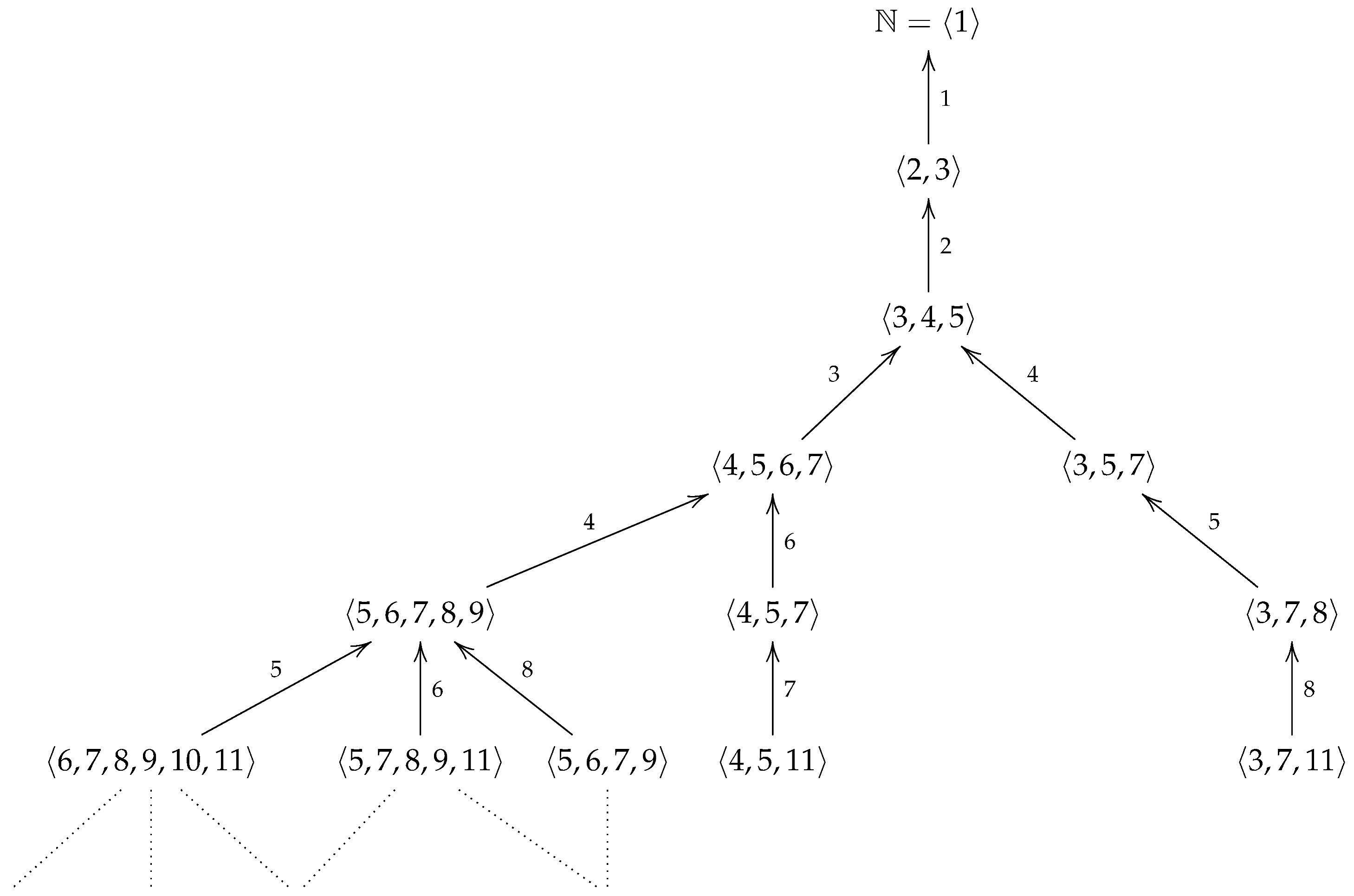
We can build a tree recursively by starting at the root and joining every constructed vertex to its children via an edge. If we use this idea and apply Theorem 1 and Proposition 2, we can construct the tree $\mathrm{G}\left(\theta \right)$ as shown below, where the number x that appears on the edge $\begin{array}{c}P\hfill \\ \uparrow x\hfill \\ Q\hfill \end{array}$ indicates that $Q=P\setminus \left\{x\right\}.$ Moreover, remark that $\mathrm{F}\left(Q\right)=x.$

Also, since the cardinality of set $\theta$ is infinite, we cannot construct the complete tree. Therefore, we will indicate this fact with ellipses.

3. Ore Semigroups with Fixed Genus

In this section our primary goal is to provide an algorithm such that given $g\in \mathbb{N}$ computes the set $\{S\mid S\mathrm{is} \mathrm{an} \mathrm{Ore} \mathrm{semigroup} \mathrm{and} \mathrm{g}(S)=g\}.$

Proposition 3.

With the above notation, it holds that $\left\{\mathrm{g}\right(S)\mid S \mathit{is} \mathit{an} \mathit{Ore} \mathit{semigroup}\}=\mathbb{N}.$

Proof. 

It suffices to observe that $S=\{0, m, \to \}$ is an Ore semigroup for all $m\in \mathbb{N}\setminus \left\{0\right\}$ and $\mathrm{g}\left(S\right)=m-1.$    □

Consider the tree $G=(V, E).$ For any vertex $v\in V,$ we denote by $\mathrm{d}\left(v\right)$ its depth, which is the length of the unique path connecting v to the root. If $k\in \mathbb{N}$, then we denote by $\mathrm{N}(G, k)=\{x\in V\mid \mathrm{d}(x)=k\}.$ The height of G is $\mathrm{h}\left(G\right)=\max \{k\in \mathbb{N}\mid \mathrm{N}(G, k)\ne Ø\}.$

Proposition 4.

If $k\in \mathbb{N},$ then the following conditions hold.

1. 

$\mathrm{N}\left(G\right(\theta ), k)=\{S\mid S \mathit{is} \mathit{an} \mathit{Ore} \mathit{semigroup} \mathit{and} \mathrm{g}(S)=k\}.$

2. 

$\mathrm{N}\left(G\right(\theta ), k+1)=\{S\mid S\mathit{is}a\mathit{child}\mathit{of}\mathit{an}\mathit{element}\mathit{of}N(G\left(\theta \right), k) \mathit{in}\mathit{the}\mathit{tree} \mathrm{G}(\theta \left)\right\}.$

Proof. 

We begin by making some observations that will assist in the proof of the proposition.

(1)

From Theorem 3, we know that $\mathrm{G}\left(\theta \right)$ is a tree with root $\mathbb{N}.$

(2)

Given $(S, T)\in \theta \times \theta$ an edge of $\mathrm{G}\left(\theta \right),$ then $T=S\cup \left\{\mathrm{F}\right(S\left)\right\},$ so $\mathrm{g}\left(S\right)=\mathrm{g}\left(T\right)+1.$

(3)

If $\mathrm{d}\left(S\right)=k,$ then the unique path connecting S with the root $\mathbb{N}$ has the length $k.$ That is, there exists $(S_0, S_1), \dots , (S_{k-1}, S_k),$ where $S_0=S$ and $S_k=\mathbb{N}.$ Therefore, as $\mathrm{g}\left(\mathbb{N}\right)=0$ and by observation (2), we have $\mathrm{g}\left(S\right)=k.$

With these observations in hand, we now proceed to the proof of the proposition.

1.

From the above and by definition, it follows that $\mathrm{N}\left(G\right(\theta ), k)=\{S\mid S\in \theta \mathrm{and} \mathrm{d}(S)=k\}=\{S\mid S \text{is an Ore semigroup and} \mathrm{g}(S)=k\}.$

2.

By combining (1) with the above remarks, it is verified that

$$\mathrm{N}\left(G\right(\theta ), k+1)=\{S\mid S \text{is an Ore semigroup and} \mathrm{g}(S)=k+1\}.$$

Hence, S is a son of a vertex T with $\mathrm{g}\left(T\right)=k.$ That is, T is a vertex reachable from the root via a path of length $k.$ So, $\mathrm{d}\left(T\right)=k.$ Therefore, $T\in \mathrm{N}\left(G\right(\theta ), k).$ Consequently,

$$\mathrm{N}\left(G\right(\theta ), k+1)=\{S\mid S\mathrm{is}\mathrm{a}\mathrm{child}\mathrm{of}\mathrm{an}\mathrm{element}\mathrm{of}\mathrm{N}(G\left(\theta \right), k) \mathrm{in}\mathrm{the}\mathrm{tree} \mathrm{G}(\theta \left)\right\}.$$

   □

We are now in a position to provide the Algorithm 1 announced at the beginning of this section.

Algorithm 1 Computation of $\{S\mid S \text{is an Ore semigroup and} \mathrm{g}(S)=g\}$

Input: A non-negative integer $g.$ Output: $\left\{S\right|S \text{is an Ore semigroup and} \mathrm{g}\left(S\right)=g\}.$ (1) $A=\mathbb{N},$ $i=0.$ (2) If $i=g$, then return A and stop. (3) For every $S\in A$ computes $\alpha \left(S\right)=\{x\in \mathrm{msg}(S\left)\right|x>\mathrm{F}\left(S\right)\mathrm{and}x=\mathrm{F}\left(S\right)+1 \mathrm{or} x \mathrm{is} \mathrm{even}\}.$ (4) ${\displaystyle A:=\bigcup _{S\in A}\{S\setminus \left\{x\right\}\mid x\in \alpha \left(S\right)\},}$ $i:=i+1$ and go to Step $\left(2\right).$

Let us see how this algorithm works.

Example 1.

We will determine the set $\{S\mid S\mathit{is} \mathit{an} \mathit{Ore} \mathit{semigroup} \mathit{and} \mathrm{g}(S)=4\}$ by applying Algorithm 1 as follows:

• $A=\left\{\mathbb{N}\right\}$, $i=0$.
• $\alpha \left(\mathbb{N}\right)=\left\{1\right\}$.
• $A=\{⟨2, 3⟩\}$, $i=1$.
• $\alpha (⟨2, 3⟩)=\left\{2\right\}$.
• $A=\{⟨3, 4, 5⟩\}$, $i=2$.
• $\alpha (⟨3, 4, 5⟩)=\{3, 4\}$.
• $A=\{⟨4, 5, 6, 7⟩, ⟨3, 5, 7⟩\}$, $i=3$.
• $\alpha (⟨4, 5, 6, 7⟩)=\{4, 6\}$ and $\alpha (⟨3, 5, 7⟩)=\left\{5\right\}.$
• $A=\{⟨5, 6, 7, 8, 9⟩, ⟨4, 5, 7⟩, ⟨3, 7, 8⟩\}$, $i=4$.
• $\{S\mid S \mathit{is} \mathit{an} \mathit{Ore} \mathit{semigroup} \mathit{and} \mathrm{g}(S)=4\}=\{⟨5, 6, 7, 8, 9⟩, ⟨4, 5, 7⟩, ⟨3, 7, 8⟩\}$.

4. Ore System of Generators

In this entire section, X stands for a non-empty subset of $\mathbb{N}\setminus \left\{0\right\}$, and we denote it by $\theta \left(X\right)=\{S\mid S \mathrm{is} \mathrm{an} \mathrm{Ore} \mathrm{semigroup} \mathrm{and} X\subseteq S\}.$ Our first objetive in this section will be to see that $\theta \left(X\right)$ is a Frobenius variety with finite cardinality.

Since $\mathbb{N}\setminus S$ is finite for any numerical semigroup $S,$ hence the following result follows.

Lemma 3.

If S is a numerical semigroup, then $\{T\mid T \mathit{is} \mathit{an} \mathit{numerical} \mathit{semigroup} \mathit{and} S\subseteq T\}$ is a finite set.

Lemma 4.

With the above notation, $\theta \left(X\right)$ is a finite set.

Proof. 

If $x\in X$ and $S\in \theta \left(X\right),$ then $\{x, 2x+1\}\subseteq S$ and so $⟨x, 2x+1⟩\subseteq S.$ As $\gcd (x, 2x+1)=1,$ then $⟨x, 2x+1⟩$ is a numerical semigroup. Consequently, $\theta \left(X\right)\subseteq \{S\mid S \mathrm{is} \mathrm{an} \mathrm{numerical} \mathrm{semigroup} \mathrm{and} ⟨x, 2x+1⟩\subseteq S\}.$ Applying Lemma 3, we can conclude that $\theta \left(X\right)$ is a finite set.    □

Proposition 5.

Using the notation above, $\theta \left(X\right)$ is a Frobenius variey with finite cardinality.

Proof. 

The following is verified.

1.

If $\{S, T\}\subseteq \theta \left(X\right),$ then $\{S, T\}\subseteq \theta$ and $X\subseteq S,$ $X\subseteq T.$ By Proposition 1, we have that $S\cap T\in \theta ,$ as $X\subseteq S\cap T;$ consequently, $S\cap T\in \theta \left(X\right).$

2.

If $S\in \theta \left(X\right)$ and $S\ne \mathbb{N},$ then $S\in \theta$ and, by Proposition 1, we have $S\cup \left\{\mathrm{F}\right(S\left)\right\}\in \theta .$ As $X\subseteq S,$ it is verified that $X\subseteq S\cup \left\{\mathrm{F}\right(S\left)\right\}.$ Therefore, $S\cup \left\{\mathrm{F}\right(S\left)\right\}\in \theta \left(X\right).$

Consequently, $\theta \left(X\right)$ is a Frobenius variety, and by Lemma 4, we obtain the result.    □

If we denote ${\displaystyle \theta \left[X\right]=\bigcap _{S\in \theta \left(X\right)}S}$ then, as a consequence of Proposition 5, we have the following.

Corollary 1.

$\theta \left[X\right]$ is the smallest, with respect to inclusion order, Ore semigroup containing $X.$

If $S=\theta \left[X\right],$ then we say that X is an Ore system of generators of $S.$ Additionally, $S\ne \theta \left[Y\right]$ for all $Y⊊X,$ then X is an Ore minimal system of generators of $S.$

By Proposition 1, we known that the set of Ore semigroups is a Frobenius variety; then by applying Corollary 19 from [22] we obtain the following result.

Theorem 2.

Every Ore semigroup has a unique Ore minimal system of generators.

If S is an Ore semigroup, then we denote by $\theta \mathrm{msg}\left(S\right)$ the Ore minimal system of generators of $S.$ The $\theta \mathrm{rank}$ of S, denoted by $\theta \mathrm{rank}\left(S\right)$ is defined as the cardinality of $\theta \mathrm{msg}\left(S\right).$

From Proposition 1 and ([22] Proposition 24), we deduce the following result which describes the Ore minimal system generator of an Ore semigroup S.

Proposition 6.

If S is an Ore semigroup, then

$$\theta \mathrm{msg}\left(S\right)=\{x\in \mathrm{msg}(S)\mid S\setminus \{x\left\} \mathit{is} \mathit{an} \mathit{Ore} \mathit{semigroup}\right\}.$$

As a consequence from Proposition 6, we have the following result.

Corollary 2.

If S is an Ore semigroup, then $\theta \mathrm{msg}\left(S\right)=\{x\in \mathrm{msg}(S)\mid x \mathit{is} \mathit{even} \mathit{or} x-1\notin S\}.$

Example 2.

Clearly, $S=\{0, 5, 7, \to \}$ is an Ore semigroup and $\mathrm{msg}\left(S\right)=\{5, 7, 8, 9, 11\}.$ By applying Corollary 2, we have $\theta \mathrm{msg}\left(S\right)=\{5, 7, 8\}$ and so $\theta \mathrm{rank}\left(S\right)=3.$

We conclude this section by providing an algorithm to compute $\theta \left[X\right],$ X being a finite and non-empty subset of $\mathbb{N}\setminus \left\{0\right\}.$ With this in mind, we first introduce some concepts and results.

Let M be a submonoid of $(\mathbb{N},+).$ Denote by ${\mathrm{msg}}_{\mathrm{e}}\left(S\right)=\{x\in \mathrm{msg}\left(S\right)\mid x \mathrm{is} \mathrm{even}\}$ and ${\mathrm{msg}}_{\mathrm{o}}\left(S\right)=\{x\in \mathrm{msg}\left(S\right)\mid x \mathrm{is} \mathrm{odd}\}.$

Let A and B be a non-empty subsets of $\mathbb{Z}$. Denote $A+B=\{a+b\mid a\in A, b\in B\}.$ Another characterization of Ore semigroups is shown in the result below.

Proposition 7.

Let S be a numerical semigroup. Then S is an Ore semigroup if and only if ${\mathrm{msg}}_{\mathrm{e}}\left(S\right)+\left\{1\right\}\subseteq S$ and ${\mathrm{msg}}_{\mathrm{o}}\left(S\right)+{\mathrm{msg}}_{\mathrm{o}}\left(S\right)+\left\{1\right\}\subseteq S.$

Proof. 

The necessary condition is trivial. Let us examine the sufficient condition. Toward this goal, we shall show that if $s\in S\setminus \left\{0\right\}$ and s is even, then $s+1\in S.$ To verify this, we consider two cases:

(1)

If there is $a\in {\mathrm{msg}}_{\mathrm{e}}\left(S\right)$ such that $s-a\in S,$ then $s+1=(s-a)+a+1\in S.$

(2)

If there is no $a\in {\mathrm{msg}}_{\mathrm{e}}\left(S\right)$ such that $s-a\in S,$ then we deduce that there exists $\{a, b\}\subseteq {\mathrm{msg}}_{\mathrm{o}}\left(S\right)$ such that $s-(a+b)\in S.$ Therefore, $s+1=(s-(a+b\left)\right)+a+b+1\in S.$

   □

We are now in a position to present the Algorithm 2 previously announced.

Algorithm 2 Computation of $\theta \left[X\right]$

Input: A finite and non-empty subset X of $\mathbb{N}\setminus \left\{0\right\}.$ Output: $\theta \left[X\right].$ (1) $S=⟨X⟩.$ (2) Compute ${\mathrm{msg}}_{\mathrm{e}}\left(S\right)$ and ${\mathrm{msg}}_{\mathrm{o}}\left(S\right).$ (3) $A=\{x\in {\mathrm{msg}}_{\mathrm{e}}\left(S\right)+\left\{1\right\}\mid x\notin S\}$ and $B=\{x\in {\mathrm{msg}}_{\mathrm{o}}\left(S\right)+{\mathrm{msg}}_{\mathrm{o}}\left(S\right)+\left\{1\right\}\mid x\notin S\}.$ (4) If $A=B=Ø,$ then return S and stop. (5) $S=⟨\mathrm{msg}\left(S\right)\cup A\cup B⟩$ and go to Step $\left(2\right).$

In what follows, we show the step-by-step operation of the previous algorithm.

Example 3.

By using Algorithm 2, let us calculate $\theta \left[\right\{5, 8\left\}\right].$

• $S=⟨5, 8⟩,$ ${\mathrm{msg}}_{\mathrm{e}}\left(S\right)=\left\{8\right\}$ and ${\mathrm{msg}}_{\mathrm{o}}\left(S\right)=\left\{5\right\}.$
• $A=\left\{9\right\}$ and $B=\left\{11\right\}.$
• $S=⟨5, 8, 9, 11⟩.$
• ${\mathrm{msg}}_{\mathrm{e}}\left(S\right)=\left\{8\right\}$ and ${\mathrm{msg}}_{\mathrm{o}}\left(S\right)=\{5, 9, 11\}.$
• $A=Ø$ and $B=Ø.$
• $\theta \left[\right\{5, 8\left\}\right]=⟨5, 8, 9, 11⟩.$

5. Ore Semigroup with $\mathit{\theta }\mathrm{rank}$ One

In this section, we will study the Ore semigroups of $\theta$rank one, that is, Ore semigroups of the form $\theta \left[\right\{m\left\}\right],$ where $m\in \mathbb{N}\setminus \left\{0\right\}.$ For this study, the proof is split into two cases, depending on the parity of $m.$

5.1. The Case Where m Is Odd

Throughout this subsection, we assume that m is an odd positive integer.

We begin by presenting a system of generators for the semigroup $\theta \left[\right\{m\left\}\right]$.

Proposition 8.

If m is odd, then $\theta \left[\right\{m\left\}\right]=⟨m, 2m+1, 3m+2, \dots , mm+m-1⟩.$

Proof. 

We use induction on i to prove that $im+i-1\in \theta \left[\right\{m\left\}\right]$ for all $i\in \{1, \dots , m\}.$ If $i=1,$ then $im+i-1=m\in \theta \left[\right\{m\left\}\right].$ Assume that $im+i-1\in \theta \left[\right\{m\left\}\right]$ and let us prove that $(i+1)m+i\in \theta \left[\right\{m\left\}\right].$ As $im+i-1$ and m are odd elements from $\theta \left[\right\{m\left\}\right]$ and $\theta \left[\right\{m\left\}\right]$ is an Ore semigroup, then $im+i-1+m+1\in \theta \left[\right\{m\left\}\right].$ Therefore, $(i+1)m+i\in \theta \left[\right\{m\left\}\right].$

If we verify that $S=⟨m, 2m+1, 3m+2, \dots , mm+m-1⟩$ is an Ore semigroup, then by applying Corollary 1, we have the result and the proof ends. Note that to prove that S is an Ore semigroup, by Proposition 7, it is enough to see that $\{m, 2m+1, \dots , mm+m-1\}+\{m, 2m+1, \dots , mm+m-1\}+\left\{1\right\}\subseteq S$ (observe that $im+i-1=i(m+1)-1$ is an odd number). To demostrate this fact, let $i, j\in \{1, \dots , m\}$; we must also distinguish two cases:

1.

If $i+j\le m,$ then $im+i-1+jm+j-1+1=(i+j)m+(i+j-1)\in S.$

2.

If $i+j>m,$ then $im+i-1+jm+j-1+1=(i+j)m+i+j-1=(i+j-m+m)m+i+j-m+m-1=(i+j-m)m+(i+j-m-1)+m^2+m\in S.$

   □

In Corollary 3, we will show that this system of generators constitutes the minimal system of generators of $\theta \left[\right\{m\left\}\right].$ To continue our study we need to introduce the concept of Apéry set and show some of its properties.

Let S be a numerical semigroup and $n\in S\setminus \left\{0\right\}.$ The Apéry set of n in S (see [25]) is $Ap(S, n)=\{s\in S\mid s-n\notin S\}.$  

The following result is deduced from ([1] Lemma 2.4).

Lemma 5.

Given S a numerical semigroup and $n\in S\setminus \left\{0\right\},$ it is verified that $\mathrm{Ap}(S, n)=\{0=w(0), w(1), \dots , w(n-1\left)\right\}$, where $w\left(i\right)$ is the least element in S congruent to i modulo n, for all $i\in \{0, \dots , n-1\}.$

The next result is deduced from ([26] Lemma 3.3).

Lemma 6.

Let $n\in \mathbb{N}\setminus \{0, 1\}$ and $\left\{\alpha \right(0)=0, \alpha (1), \dots , \alpha (n-1\left)\right\}\subseteq \mathbb{N}$ such that $\alpha \left(i\right)$ is congruent to i modulo n for all $i\in \{0, \dots , n-1\}$ and let $S=⟨n, \alpha \left(1\right), \dots , \alpha (n-1)⟩.$ Then $\mathrm{Ap}(S, n)=\left\{\alpha \right(0), \alpha (1), \dots , \alpha (n-1\left)\right\}$ if and only if $\alpha \left(i\right)+\alpha \left(j\right)\ge \alpha \left(\right(i+j\left) \mathit{mod} n\right)$ for all $\{i, j\}\subseteq \{1, \dots , n-1\}.$

Proposition 9.

If m is odd, then $\mathrm{Ap}\left(\theta \right[\left\{m\right\}], m)=\{0, 2m+1, 3m+2, \dots , mm+m-1\}.$

Proof. 

According to Proposition 8 and Lemma 6, it suffices to show that $\{i, j\}\subseteq \{1, \dots , m-1\}$ and $i+j\ne m,$ then $(i+1)m+i+(j+1)m+j\ge \left(\left(\right(i+j\left) \mathrm{mod} m\right)+1\right)m+(i+j) \mathrm{mod} m.$ But it is true because $(i+1)m+i+(j+1)m+j=(i+j+2)m+i+j>\left(\left(\right(i+j\left) \mathrm{mod} m\right)+1\right)m+(i+j) \mathrm{mod} m.$    □

Recall that if we denote by $\mathrm{msg}\left(S\right)$ the minimal system of generators of a numerical semigroup $S,$ then $\mathrm{e}\left(S\right)$ and $\mathrm{m}\left(S\right)$ denote the embedding dimension and the multiplicity of S, that is, the cardinality and the minimum of $\mathrm{msg}\left(S\right),$ respectively. Given a numerical semigroup S, from Proposition 2.10 in [1], we know that $\mathrm{e}\left(S\right)\le m\left(S\right).$ A numerical semigroup S has maximal embedding dimension if $\mathrm{e}\left(S\right)=\mathrm{m}\left(S\right).$

In ([1] Corollary 2.6) appears the following result.

Lemma 7.

Let S be a numerical semigroup, $\mathrm{m}\left(S\right)=n$ and $\mathrm{Ap}(S, n)=\left\{w\right(0)=0, w(1), \dots , w(n-1\left)\right\}.$ Then S has maximal embedding dimension if and only if $w\left(i\right)+w\left(j\right)>w\left(\right(i+j\left)modn\right)$ for all $\{i, j\}\subseteq \{1, \dots , n-1\}.$

By applying Lemma 7, Proposition 9 and the end of its proof, we deduce the following.

Proposition 10.

If m is odd, then the numerical semigroup $\theta \left[\right\{m\left\}\right]$ has maximal embedding dimension.

Finally, the following result which is a consequence from Propositions 8 and 10, presents the minimal generator system for Ore semigroups of the form $\theta \left[\right\{m\left\}\right],$ where m is odd.

Corollary 3.

If m is odd, then $\{m, 2m+1, 3m+2, \dots , mm+m-1\}$ is the minimal system of generators of $\theta \left[\right\{m\left\}\right].$

In order to calculate the genus of $\theta \left[\right\{m\left\}\right],$ where m is odd, we recall the following result that appears in [27].

Lemma 8.

If S is a numerical semigroup and $n\in S\setminus \left\{0\right\},$ then $\mathrm{F}\left(S\right)=\max \left(\mathrm{Ap}(S, n)\right)-n$ and ${\displaystyle \mathrm{g}\left(S\right)=\frac{1}{n}\sum _{w\in \mathrm{Ap}(S, n)}w-\frac{n-1}{2}.}$

We are now in a position to determine the embedding dimension, the multiplicity, the Frobenius number and the genus of $\theta \left[\right\{m\left\}\right]$, assuming m is odd.

Theorem 3.

If m is odd, then $\mathrm{e}\left(\theta \right[\left\{m\right\}\left]\right)=\mathrm{m}\left(\theta \right[\left\{m\right\}\left]\right)=m,$ $\mathrm{F}\left(\theta \left[\right\{m\left\}\right]\right)=m^2-1$ and ${\displaystyle \mathrm{g}\left(\theta \left[\right\{m\left\}\right]\right)=\frac{(m+2)(m-1)}{2}.}$

Proof. 

By Corollary 3, we know that $\mathrm{e}\left(\theta \right[\left\{m\right\}\left]\right)=\mathrm{m}\left(\theta \right[\left\{m\right\}\left]\right)=m.$ By applying Proposition 9 and Lemma 8, we can easily deduce that $\mathrm{F}\left(\theta \left[\right\{m\left\}\right]\right)=mm+m-1-m=m^2-1$ and ${\displaystyle \mathrm{g}\left(\theta \left[\right\{m\left\}\right]\right)=\frac{1}{m}[(2m+1)+(3m+2)+\dots +(mm+m-1)]-\frac{m-1}{2}=\frac{1}{m}[(m(2+3+\dots +m)+(1+2+\dots +m-1)]-\frac{m-1}{2}=\frac{1}{m}\left[{\displaystyle m\frac{(m+2)(m-1)}{2}+\frac{m(m-1)}{2}}\right]-\frac{m-1}{2}=\frac{(m+2)(m-1)}{2}.}$    □

Now we illustre the previous result.

Example 4.

By Corollary 3, we know that $\{5, 11, 17, 23, 29\}$ is the minimal system of generators of $\theta \left[\right\{5\left\}\right]$ and by using Theorem 3, it is verified that $\mathrm{F}\left(\theta \left[\right\{5\left\}\right]\right)=5^2-1=24$ and $\mathrm{g}\left(\theta \left[\right\{5\left\}\right]\right)={\displaystyle \frac{7·4}{2}}=14.$

5.2. The Case Where m Is Even

We now turn our attention to the study of $\theta \left[\right\{m\left\}\right]$ when m is even. Therefore, throughout this subsection, we shall assume that m is a positive even integer.

Our first result yields a system of generators for $\theta \left[\right\{m\left\}\right]$.

Proposition 11.

If m is even, then $\theta \left[\left\{m\right\}\right]=⟨m, m+1, 2m+3, \dots , {\displaystyle \frac{m}{2}}m+m-1⟩.$

Proof. 

We use, once more, induction on i to prove that $im+2i-1\in \theta \left[\right\{m\left\}\right]$ for all $i\in \{1, \dots , {\displaystyle \frac{m}{2}}\}.$ For $i=1$ the result is obvious. By induction hypothesis, $im+2i-1\in \theta \left[\right\{m\left\}\right]$ and so $im+2i-1+m+1$ is an even element of $\theta \left[\right\{m\left\}\right].$ As $\theta \left[\right\{m\left\}\right]$ is an Ore semigroup, then $im+2i-1+m+1+1\in \theta \left[\right\{m\left\}\right]$ and consequently, $(i+1)m+2(i+1)-1\in \theta \left[\right\{m\left\}\right].$

By applying Corollary 1 to conclude the proof, it will be enough that $S=⟨m, m+1, 2m+3, \dots , {\displaystyle \frac{m}{2}}m+m-1⟩$ is an Ore semigroup. To do this, by virtue of Proposition 7, it will suffice to see that $\{m+1, 2m+3, \dots , {\displaystyle \frac{m}{2}}m+m-1\}+\{m+1, 2m+3, \dots , {\displaystyle \frac{m}{2}}m+m-1\}+\left\{1\right\}\subseteq S.$ Indeed, let $\{i, j\}\subseteq \{1, \dots , {\displaystyle \frac{m}{2}}\}$ and we will see that $im+2i-1+jm+2j-1+1\in S.$ To this purpose, we distinguish between two cases.

1.

If $i+j\le {\displaystyle \frac{m}{2}},$ then $im+2i-1+jm+2j-1+1=(i+j)m+2(i+j)-1\in \{2m+3, \dots , {\displaystyle \frac{m}{2}}m+m-1\}\subseteq S.$

2.

If $i+j>m,$ then $im+2i-1+jm+2j-1+1=(i+j-{\displaystyle \frac{m}{2}}+{\displaystyle \frac{m}{2}})m+2(i+j-{\displaystyle \frac{m}{2}}+{\displaystyle \frac{m}{2}})-1=(i+j-{\displaystyle \frac{m}{2}})m+2(i+j-{\displaystyle \frac{m}{2}})-1+{\displaystyle \frac{m}{2}}m+m\in S.$

   □

Our study now aims to show that the system of generators for $\theta \left[\right\{m\left\}\right]$ presented above is, in fact, its minimal system of generators. This result will be the content of Corollary 4. The Apéry set, as in the case of odd $m,$ will be a fundamental tool for achieving this goal.

Proposition 12.

If m is even, then $\mathrm{Ap}(\theta \left[\left\{m\right\}\right], m)=\{0, m+1, 2m+2, 2m+3, 3m+4, 3m+5, \dots , {\displaystyle \frac{m}{2}}m+m-2, {\displaystyle \frac{m}{2}}m+m-1\}.$

Proof. 

Let $\alpha \left(0\right)=0,$ $\alpha \left(1\right)=m+1,$ $\alpha \left(2\right)=2m+2,$ $\alpha \left(3\right)=2m+3,$ $\alpha \left(4\right)=3m+4,$ $\alpha \left(5\right)=3m+5, \dots , \alpha (m-2)={\displaystyle \frac{m}{2}}m+m-2$ and $\alpha (m-1)={\displaystyle \frac{m}{2}}m+m-1.$ Note that for every $i\in \{1, \dots , m-1\}$ we have

$$\alpha \left(i\right)=\left\{\begin{array}{ccc}{\displaystyle \frac{i+1}{2}}m+i\hfill & \mathrm{if}& i \mathrm{is} \mathrm{odd},\hfill \\ {\displaystyle \frac{i+2}{2}}m+i\hfill & \mathrm{if}& i \mathrm{is} \mathrm{even}.\hfill \end{array}\right.$$

If i is odd, then by Proposition 11, $\alpha \left(i\right)\in \theta \left[\right\{m\left\}\right].$ Now we will see that if i is even, then also $\alpha \left(i\right)\in \theta \left[\right\{m\left\}\right].$ Indeed, $\left\{\alpha \right(i-1), m+1\}\subseteq \theta \left[\right\{m\left\}\right]$ and so $\alpha (i-1)+m+1\in \theta \left[\right\{m\left\}\right].$ Therefore, ${\displaystyle \frac{i-1+1}{2}}m+i-1+m+1\in \theta \left[\left\{m\right\}\right]$ and consequently, $\alpha \left(i\right)={\displaystyle \frac{i+2}{2}}m+i\in \theta \left[\left\{m\right\}\right].$

To complete the proposition, it will suffice to see, by Lemma 6, that $\alpha \left(i\right)+\alpha \left(j\right)\ge \alpha \left(\right(i+j\left) \mathrm{mod} m\right)$ for all $\{i, j\}\subseteq \{1, \dots , m-1\}.$ Three cases can be identified for this purpose.

1.

If i and j are odd, then $\alpha \left(i\right)+\alpha \left(j\right)={\displaystyle \frac{i+1}{2}}m+i+{\displaystyle \frac{j+1}{2}}m+j={\displaystyle \frac{i+j+2}{2}}m+i+j\ge {\displaystyle \frac{(i+j) \mathrm{mod} m+2}{2}}m+(i+j) \mathrm{mod} m=\alpha \left((i+j) \mathrm{mod} m\right).$

2.

If i and j are even, then $\alpha \left(i\right)+\alpha \left(j\right)={\displaystyle \frac{i+2}{2}}m+i+{\displaystyle \frac{j+2}{2}}m+j={\displaystyle \frac{i+j+4}{2}}m+i+j>{\displaystyle \frac{(i+j) \mathrm{mod} m+2}{2}}m+(i+j) \mathrm{mod} m=\alpha \left((i+j) \mathrm{mod} m\right).$

3.

If i is odd and j is even, then $\alpha \left(i\right)+\alpha \left(j\right)={\displaystyle \frac{i+1}{2}}m+i+{\displaystyle \frac{j+2}{2}}m+j={\displaystyle \frac{i+j+3}{2}}m+i+j>{\displaystyle \frac{(i+j) \mathrm{mod} m+1}{2}}m+(i+j) \mathrm{mod} m=\alpha \left((i+j) \mathrm{mod} m\right).$

   □

Note that as a consequence of case 3 in the proof of Proposition 12, it follows that if i is odd, then $\alpha \left(i\right)$ cannot be expressed as $\alpha \left(i\right)+\alpha \left(j\right)$ being $\{i, j\}\subseteq \{1, \dots , m-1\}.$ Therefore, we can state the following announced result.

Corollary 4.

If m is even, then $\{m, m+1, 2m+3, \dots , {\displaystyle \frac{m}{2}}m+m-1\}$ is the minimal system of generators of $\theta \left[\right\{m\left\}\right].$

We now have all the necessary ingredients to compute the embedding dimension, Frobenius number and genus of the semigroup $\theta \left[\right\{m\left\}\right].$

Theorem 4.

If m is even, then $\mathrm{e}\left(\theta \left[\left\{m\right\}\right]\right)={\displaystyle \frac{m}{2}}+1,$ $\mathrm{F}\left(\theta \left[\right\{m\left\}\right]\right)={\displaystyle \frac{m^2}{2}}-1$ and ${\displaystyle \mathrm{g}\left(\theta \left[\right\{m\left\}\right]\right)=\frac{1}{2}\left[\frac{m}{2}\left(\frac{m}{2}+1\right)+\left(\frac{m}{2}+2\right)\left(\frac{m}{2}-1\right)\right].}$

Proof. 

As an immediate consequence of Corollary 4, we can state that $\mathrm{e}\left(\theta \left[\left\{m\right\}\right]\right)={\displaystyle \frac{m}{2}}+1.$ By using Lemma 8 and Proposition 12, we can easily deduce that $\mathrm{F}\left(\theta \left[\right\{m\left\}\right]\right)={\displaystyle \frac{m^2}{2}}-1$ and ${\displaystyle \mathrm{g}\left(\theta \left[\right\{m\left\}\right]\right)=\frac{1}{2}\left[\frac{m}{2}\left(\frac{m}{2}+1\right)+\left(\frac{m}{2}+2\right)\left(\frac{m}{2}-1\right)\right].}$    □

Let’s look at an example of the previous result.

Example 5.

By Corollary 4, the set $\{6, 7, 15, 23\}$ is the minimal system of generators of $\theta \left[\right\{6\left\}\right]$ and by Theorem 4, we have $\mathrm{F}\left(\theta \left[\right\{6\left\}\right]\right)=17$ and $\mathrm{g}\left(\theta \left[\right\{6\left\}\right]\right)=11.$

The following result is given in ([11] Theorem 3.2).

Proposition 13.

If S is a numerical semigroup and $3\mathrm{e}\left(S\right)\ge \mathrm{m}\left(S\right),$ then S verifies the Wilf’s conjecture.

Finally, by Proposition 13 and Theorems 3 and 4, we obtain the following result where a new family of semigroups satisfying Wilf’s conjecture is identified, that is, all Ore semigroups with $\theta \mathrm{rank}$ one verifiy the Wilf’s conjecture.

Corollary 5.

If S is an Ore semigroup and $\theta \mathrm{rank}\left(S\right)=1,$ then Wilf’s conjecture holds for $S.$

6. The Ore Semigroups with Fixed Multiplicity

In this section, m will denote an integer greater than or equal to 2, and we consider the set ${\theta }_m=\{S\mid S \text{is an Ore semigroup and} \mathrm{m}\left(S\right)=m\}.$ Our main aim will be to design an algorithm that computes all the elements of ${\theta }_m$. To do this, we need to introduce the following concept.

We define a Frobenius pseudo-variety as a family $\mathcal{P}$ of numerical semigroups subject to the following conditions:

1.

$\mathcal{P}$ has a maximum (with respect to inclusion order).

2.

If $\{S, T\}\subseteq \mathcal{P},$ then $S\cap T\in \mathcal{P}.$

3.

If $S\in \mathcal{P}$ and $S\ne \max \left(\mathcal{P}\right),$ then $S\cup \left\{\mathrm{F}\right(S\left)\right\}\in \mathcal{P}.$

Proposition 14.

${\theta }_m$ is a Frobenius pseudo-variety with finite cardinality. In addition $\{0, m, \to \}$ is its maximum.

Proof. 

It is clear that $\{0, m, \to \}$ is the maximum of ${\theta }_m.$ If $\{S, T\}\subseteq {\theta }_m,$ then by Lemma 1 and Proposition 1, we deduce easily that $S\cap T\in {\theta }_m.$ Likewise, if $S\ne \{0, m, \to \},$ then $S\cup \left\{\mathrm{F}\left(S\right)\right\}\in {\theta }_m.$ Hence, ${\theta }_m$ is a Frobenius pseudo-variety.

If $S\in {\theta }_m,$ then $⟨m, 2m+1⟩\subseteq S.$ As $⟨m, 2m+1⟩$ is a numerical semigroup, then by applying Lemma 3, we assert that ${\theta }_m$ is a finite set.    □

Consider the graph $\mathrm{G}\left({\theta }_m\right),$ whose vertex set is ${\theta }_m$ and $(S, T)\in {\theta }_m\times {\theta }_m$ is an edge if and only if $T=S\cup \left\{\mathrm{F}\right(S\left)\right\}.$

In view of Proposition 14 and ([23] Theorem 3), we may state the below result.

Proposition 15.

The graph $\mathrm{G}\left({\theta }_m\right)$ is a tree where $\{0, m, \to \}$ is its root. In additon, the set of children of a vertex S in the tree $\mathrm{G}\left({\theta }_m\right)$ is given by $\{S\setminus \left\{x\right\}\mid x\in \mathrm{msg}\left(S\right),x>\mathrm{F}\left(S\right) and S\setminus \left\{x\right\}\in {\theta }_m\}.$

Proposition 16.

Let $S\in {\theta }_m$ and $x\in \mathrm{msg}\left(S\right)$ such that $x>\mathrm{F}\left(S\right).$ Then $S\setminus \left\{x\right\}\in {\theta }_m$ if and only if $x\ne m$ and x is even or $x=\mathrm{F}\left(S\right)+1.$

Proof. 

(Necessity.) If $S\setminus \left\{x\right\}\in {\theta }_m,$ then $\mathrm{m}(S\setminus \{x\left\}\right)=m$ and so $x\ne m.$ Moreover, $x-1$ is odd or $x-1\notin S.$ Therefore, x is even or $x=\mathrm{F}\left(S\right)+1.$

(Sufficiency.) By Lemma 2, we assert that $S\setminus \left\{x\right\}$ is a numerical semigroup. As $x\ne m,$ then $\mathrm{m}(S\setminus \{x\left\}\right)=m.$ It remains to show that $S\setminus \left\{x\right\}$ is an Ore semigroup to conclude the proof. For this purpose it is enough to see that if $x-1\in S,$ then $x-1$ is even. But this statement is clearly deduced from the hypotheses.    □

Subsequently, we will illustrate how the tree $\mathrm{G}\left({\theta }_5\right)$ is constructed by means of Propositions 15 and 16.

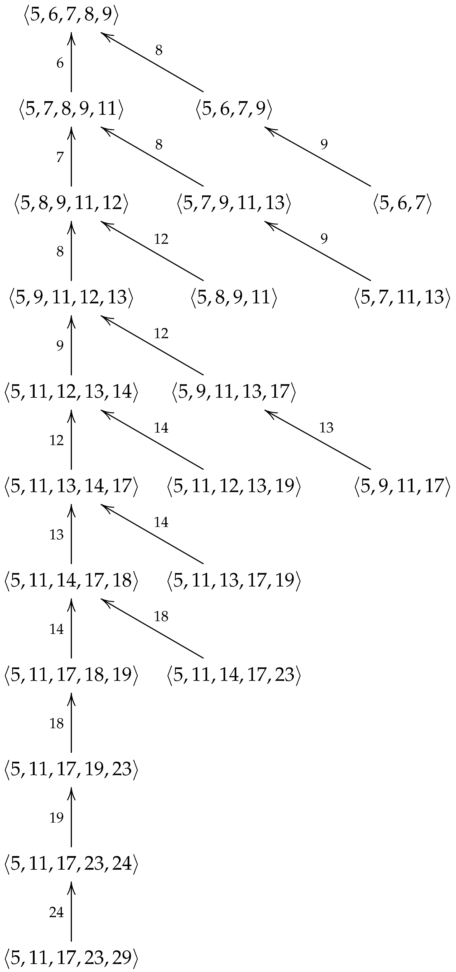
The number x, which appears on the edge $\begin{array}{c}P\hfill \\ \uparrow x\hfill \\ Q\hfill \end{array},$ indicates that $Q=P\setminus \left\{x\right\}$. Moreover, note that $\mathrm{F}\left(Q\right)=x$.

It is clear that $\min \left({\theta }_m\right)=\theta \left[\left\{m\right\}\right]$, and so we have the next outcome.

Proposition 17.

With the above notation, the following is verified

1. 

If m is odd, then ${\displaystyle \{\mathrm{g}\left(S\right)\mid S\in {\theta }_m\}=\{m-1, m, \dots , \frac{(m+2)(m-1)}{2}\}}$ and ${\displaystyle \mathrm{h}\left(\mathrm{G}\left({\theta }_m\right)\right)=\frac{m(m-1)}{2}.}$

2. 

If m is even, then ${\displaystyle \{\mathrm{g}\left(S\right)\mid S\in {\theta }_m\}=\{m-1, m, \dots , \frac{1}{2}\left[\frac{m}{2}\left(\frac{m}{2}+1\right)+\left(\frac{m}{2}+2\right)\left(\frac{m}{2}-1\right)\right]\}}$ and ${\displaystyle \mathrm{h}\left(\mathrm{G}\left({\theta }_m\right)\right)=\frac{1}{2}\left[\frac{m}{2}\left(\frac{m}{2}+1\right)+\left(\frac{m}{2}+2\right)\left(\frac{m}{2}-1\right)\right]-(m-1).}$

If $m\in \mathbb{N}\setminus \{0, 1\},$ then denote by   

$$\mathrm{g}\left(m\right)=\left\{\begin{array}{ccc}{\displaystyle \frac{(m+2)(m-1)}{2}}\hfill & \mathrm{if}\hfill & m \mathrm{is} \mathrm{odd},\hfill \\ {\displaystyle \frac{1}{2}\left[\left(\frac{m}{2}+1\right)\frac{m}{2}+\left(\frac{m}{2}+2\right)\left(\frac{m}{2}-1\right)\right]}\hfill & \mathrm{if}\hfill & m \mathrm{is} \mathrm{even}.\hfill \end{array}\right.$$

We can now provide the Algorithm 3 announced at the outset of this section.

Algorithm 3 Computation of ${\theta }_m$

Input: $m\in \mathbb{N}\setminus \{0, 1\}.$ Output: ${\theta }_m.$ (1) $A=\left\{\right\{0, m, \to \left\}\right\},$ $B=\left\{\right\{0, m, \to \left\}\right\},$ $i=m-1.$ (2) If $i=g\left(m\right)$, then return A and stop. (3) For every $S\in B$ computes $\gamma \left(S\right)=\{x\in \mathrm{msg}(S)\mid x>\mathrm{F}(S), x\ne m \mathrm{and} x \mathrm{is} \mathrm{even} \mathrm{or} x=\mathrm{F}(S)+1\}.$ (4) ${\displaystyle C:=\bigcup _{S\in B}\{S\setminus \left\{x\right\}\mid x\in \gamma \left(S\right)\}.}$ (5) $A:=A\cup C,$ $B:=C,$ $i:=i+1$ and go to Step $\left(2\right).$

Let us look at an example of how this algorithm works.

Example 6.

We obtain ${\theta }_4$ through Algorithm 3. First, we observe that $\mathrm{g}\left(4\right)=5.$

• $A=\{⟨4, 5, 6, 7⟩\},$ $B=\{⟨4, 5, 6, 7⟩\},$ $i=3.$
• $\gamma (⟨4, 5, 6, 7⟩)=\left\{6\right\}.$
• $C=\{⟨4, 5, 7⟩\}.$
• $A=\{⟨4, 5, 6, 7⟩, ⟨4, 5, 7⟩\},$ $B=\{⟨4, 5, 7⟩\},$ $i=4.$
• $\gamma (⟨4, 5, 7⟩)=\left\{7\right\}.$
• $C=\{⟨4, 5, 11⟩\}.$
• $A=\{⟨4, 5, 6, 7⟩, ⟨4, 5, 7⟩, ⟨4, 5, 11⟩\},$ $B=\{⟨4, 5, 11⟩\},$ $i=5.$
• ${\theta }_4=\{⟨4, 5, 6, 7⟩,⟨4, 5, 7⟩, ⟨4, 5, 11⟩\}.$

We will demonstrate how a slight modification to Algorithm 3 enables the computation of all elements in B belonging to a specific genus.

Let us consider an example of the operation of this Algorithm 4.

Algorithm 4 Computation of $\{S\in {\theta }_m\mid \mathrm{g}\left(S\right)=g\}$

Input: $m\in \mathbb{N}\setminus \{0, 1\}$ and $g\in \mathbb{N}.$ Output: $\{S\in {\theta }_m\mid \mathrm{g}\left(S\right)=g\}.$ (1) If $g\notin \{m-1, m, \dots , \mathrm{g}(m\left)\right\},$ then return Ø and stop. (2) $A=\left\{\right\{0, m, \to \left\}\right\},$ $i=m-1.$ (3) If $i=g$, then return A and stop. (4) For every $S\in A$ computes $\gamma \left(S\right)=\{x\in \mathrm{msg}(S)\mid x>\mathrm{F}(S), x\ne m \mathrm{and} x \mathrm{is} \mathrm{even} \mathrm{or} x=\mathrm{F}(S)+1\}.$ (5) ${\displaystyle A:=\bigcup _{S\in A}\{S\setminus \left\{x\right\}\mid x\in \gamma \left(S\right)\},}$ $i:=i+1$ and go to Step $\left(3\right).$

Example 7.

We will calculate $\{S\in {\theta }_5\mid \mathrm{g}\left(S\right)=6\}$ by using Algorithm 4. Note that $5-1\le 6\le \mathrm{g}\left(5\right)=14.$

• $A=\{⟨5, 6, 7, 8, 9⟩\},$ $i=4.$
• $\gamma (⟨5, 6, 7, 8, 9⟩)=\{6, 8\}.$
• $A=\{⟨5, 7, 8, 9, 11⟩, ⟨5, 6, 7, 9⟩\},$ $i=5.$
• $\gamma (⟨5, 7, 8, 9, 11⟩)=\{7, 8\}$ and $\gamma (⟨5, 6, 7, 9⟩)=\left\{9\right\}.$
• $A=\{⟨5, 8, 9, 11, 12⟩, ⟨5, 7, 9, 11, 13⟩, ⟨5, 6, 7⟩\},$ $i=6.$
• $\{S\in {\theta }_5\mid \mathrm{g}\left(S\right)=6\}=\{⟨5, 8, 9, 11, 12⟩, ⟨5, 7, 9, 11, 13⟩, ⟨5, 6, 7⟩\}.$

7. The Ore Semigroups with a Fixed Frobenius Number

Throughout this section, F will denote a positive integer. Our goal here is to present an algorithm that computes $\theta \left(F\right)=\{S\mid S \mathrm{is} \mathrm{an} \mathrm{Ore} \mathrm{semigroup} \mathrm{and} \mathrm{F}(S)=F\}$. To this end, we need to introduce the following concept.

We will say that a family of numerical semigroups $\mathcal{C}$ is a covariety if it satisfies the conditions below.

1.

$\mathcal{C}$ has a minimum (to respect to inclusion order).

2.

If $\{S, T\}\subseteq \mathcal{C}$ then $S\cap T\in \mathcal{C}.$

3.

If $S\in \mathcal{C}$ and $S\ne \min \left(\mathcal{C}\right),$ then $S\setminus \left\{\mathrm{m}\right(S\left)\right\}\in \mathcal{C}.$

The following result can be easily obtained by Proposition 1 and Lemma 2.

Proposition 18.

$\theta \left(F\right)$ is a covariety and $\{0, F+1, \to \}$ is its minimum.

We are going to consider the following graph $\mathrm{G}\left(\theta \right(F\left)\right)$: its vertex set will be $\theta \left(F\right)$, and we say that $(S, T)\in \theta \left(F\right)\times \theta \left(F\right)$ is an edge if and only if $T=S\setminus \left\{\mathrm{m}\right(S\left)\right\}.$

By applying Proposition 18 and ([24] Proposition 2.6), we obtain the following.

Proposition 19.

$\mathrm{G}\left(\theta \right(F\left)\right)$ is a rooted tree at $\{0, F+1, \to \}.$

We next describe the children of each vertex in the tree $\mathrm{G}\left(\theta \right(F\left)\right)$. To this end, we must first introduce the following concept.

A special gap of a numerical semigroup S is an integer x such that $x\notin S$ and $S\cup \left\{x\right\}\in S.$ We will denote by $\mathrm{S}G\left(S\right)$ the set of special gaps of $S.$ If we apply Proposition 18 and ([24] Proposition 2.9), we have the following result.

Proposition 20.

Given $S\in \theta \left(F\right),$ then the set formed by the children of S in the tree $\mathrm{G}\left(\theta \right(F\left)\right)$ is $\{S\cup \{x\}\mid x\in \mathrm{S}G(S), x<\mathrm{m}(S) \mathrm{and} S\cup \{x\}\in \theta (F\left)\right\}.$

The proof of following result is straightforward.

Proposition 21.

Let $S\in \theta \left(F\right)$ and $x\in \mathrm{S}G\left(S\right)$ such that $x<\mathrm{m}\left(S\right).$ Then $S\cup \left\{x\right\}\in \theta \left(F\right)$ if and only if $x\ne F$ and x is odd or $x=\mathrm{m}\left(S\right)-1.$

Remark 1.

Let S be a numerical semigroup and we suppose that $\mathrm{Ap}(S, n)$ is known for some $n\in S\setminus \left\{0\right\}.$ Then, the following is true:

1. 

By Remark 1 from [24], we can obtain $\mathrm{S}G\left(S\right).$

2. 

We can compute the set $\mathrm{Ap}(S\cup \{x\}, n)$ for all $x\in \mathrm{S}G\left(S\right)$ by using ([24] Remark 2).

We are now ready to show the Algorithm 5 mentioned at the start of this section.

Algorithm 5 Computation of $\theta \left(F\right)$

Input: A positive integer F. Output: $\theta \left(F\right).$ (1) $A=B=\left\{\right\{0, F+1, \to \left\}\right\}$ and $\mathrm{Ap}\left(\right\{0, F+1, \to \}, F+1)=\{0, F+2, F+3, \dots , 2F+1\}.$ (2) For every $S\in B$ computes $\lambda \left(S\right)=\{x\in \mathrm{S}G(S)\mid x\ne F, x<\mathrm{m}(S) \mathrm{and} x \mathrm{is} \mathrm{odd} \mathrm{or} x=\mathrm{m}(S)-1\}.$ (3) ${\displaystyle C:=\bigcup _{S\in B}\{S\cup \left\{x\right\}\mid x\in \lambda \left(S\right)\}.}$ (4) If $C=Ø,$ then return A and stop. (5) $A:=A\cup C$ and $B:=C.$ (6) For all $S\in B$ compute $\mathrm{Ap}(S, F+1)$ and go to Step $\left(2\right).$

This section and the paper end by showing how all semigroups with a specific Frobenius number can be obtained through the application of the previous algorithm.

Example 8.

We are going to computes $\theta \left(7\right)$ by using Algorithm 5.

• $A=B=\left\{\right\{0, 8, \to \left\}\right\}$ and $\mathrm{Ap}\left(\right\{0, 8, \to \}, 8)=\{0, 9, 10, 11, 12, 13, 14, 15\}.$
• $\lambda \left(\right\{0, 8, \to \left\}\right)=\left\{5\right\}.$
• $C=\left\{\right\{0, 5, 8, \to \left\}\right\}.$
• $A=\left\{\right\{0, 5, 8, \to \}, \{0, 8, \to \left\}\right\}$ and $B=\left\{\right\{0, 5, 8, \to \left\}\right\}.$
• $\mathrm{Ap}\left(\right\{0, 5, 8, \to \}, 8)=\{0, 5, 9, 10, 11, 12, 14, 15\}.$
• $\lambda \left(\right\{0, 5, 8, \to \left\}\right)=\left\{4\right\}.$
• $C=\left\{\right\{0, 4, 5, 8, \to \left\}\right\}.$
• $A=\left\{\right\{0, 4, 5, 8, \to \}, \{0, 5, 8, \to \}, \{0, 8, \to \left\}\right\}$ and $B=\left\{\right\{0, 4, 5, 8, \to \left\}\right\}.$
• $\mathrm{Ap}\left(\right\{0, 4, 5, 8, \to \}, 8)=\{0, 4, 5, 9, 10, 11, 14, 15\}.$
• $\lambda \left(\right\{0, 4, 5, 8, \to \left\}\right)=Ø.$
• $C=Ø.$
• $\theta \left(7\right)=\left\{\right\{0, 4, 5, 8, \to \}, \{0, 5, 8, \to \}, \{0, 8, \to \left\}\right\}.$

8. Conclusions

The content of this work falls within the field of number theory, using combinatorial techniques for this purpose. We aimed to provide a modest contribution toward resolving three significant open problems in the theory of numerical semigroups: the Frobenius problem, the conjecture of Bras-Amorós and Wilf’s conjecture.

The notion of the Ore semigroup is introduced in this work. We establish that the collection of all Ore semigroups constitutes a variety; furthermore, we develop an algorithm for computing all such semigroups with a specified genus.

If X is a subset of $\mathbb{N}\setminus \left\{0\right\},$ then we demostrate that there is a smallest Ore semigroup that contains it, denoted by $\theta \left[X\right].$ If S is an Ore semigroup and $S=\theta \left[X\right],$ then X is called an Ore minimal system of generators. We have tested that every Ore semigroup has a unique Ore minimal system of generators, denoted by $\theta \mathrm{msg}\left(S\right)$, and its cardinality is called $\theta \mathrm{rank}$ of $S.$ The work presents a detailed study of Ore semigroups with $\theta \mathrm{rank}$ one, demonstrating that they verify Wilf’s conjecture.

Finally, we demonstrate that the set all Ore semigroups with a given multiplicity (Frobenius number) is a Frobenius pseudo-variety (respectively, a covariety), presenting an algorithm to calculate all of them.

References

- Rosales, J.C.; García-Sánchez, P.A. Numerical Semigroups; Springer: New York, NY, USA, 2009; Volume 20. [Google Scholar]
- Ramírez Alfonsín, J.L. The Diophantine Frobenius Problem; Oxford University Press: London, UK, 2005. [Google Scholar]
- Sylvester, J.J. Problem 7382. Educ. Times J. Coll. Preceptors New Ser. 1883, 36, 177. [Google Scholar]
- Brauer, A. On a problem of partitions. Amer. J. Math. 1942, 64, 299–312. [Google Scholar] [CrossRef] [Scilit]
- Curtis, F. On formulas for the Frobenius number of a numerical semigroup. Math. Scand. 1990, 67, 190–192. [Google Scholar] [CrossRef] [Scilit]
- Davison, J.L. On the linear Diophantine problem of Frobenius. J. Number Theory 1994, 48, 353–363. [Google Scholar] [CrossRef] [Scilit]
- Djawadi, M.; Hofmeister, G. Linear Diophantine problem. Arch. Math 1996, 66, 19–29. [Google Scholar] [CrossRef] [Scilit]
- Johnson, S.M. A linear diophantine problem. Canadian J. Math. 1960, 12, 390–398. [Google Scholar] [CrossRef] [Scilit]
- Watanabe, K. Some examples of one dimensional Gorenstein domains. Nagoya Math. J. 1973, 49, 101–109. [Google Scholar] [CrossRef] [Scilit]
- Wilf, H.S. A circle-of-lights algorithm for the “money-change problem”. Amer. Math. Mon. 1978, 85, 562–565. [Google Scholar]
- Delgado, M. Conjeture of Wilf: A survey. In Numerical Semigroups; INdAM Series; Springer: Cham, Switzerland, 2020; Volume 40, pp. 39–62. [Google Scholar]
- Delgado, M.; Eliahou, S.; Fromentin, A. A verification of Wilf’s conjeture up to genus 100. J. Algebra 2025, 664, 150–163. [Google Scholar] [CrossRef] [Scilit]
- Eliahou, S. Wilf’s conjeture and Macaulay’s Theorem. J. Eur. Math. Soc. 2018, 20, 2105–2129. [Google Scholar] [CrossRef] [Scilit]
- Eliahou, S. A graph-theoretic approach to Wilf’s conjeture. Elec. J. Combin. 2020, 27, 15–31. [Google Scholar] [CrossRef] [Scilit]
- Eliahou, S.; Fromentin, J. Near-misses in Wilf’s conjeture. Semigroup Forum 2019, 98, 285–298. [Google Scholar]
- Blanco, V.; Rosales, J.C. The set of numerical semigroups of a given genus. Semigroup Forum 2012, 85, 255–267. [Google Scholar] [CrossRef] [Scilit]
- Bras-Amorós, M. Bound on the number of numerical semigroups of a given genus. J. Pure Appl. Algebra 2008, 213, 997–1001. [Google Scholar]
- Bras-Amorós, M. Fibonacci-like behavior of the number of numerical semigroups of a given genus. Semigroup Forum 2008, 76, 379–384. [Google Scholar]
- Elizalde, S. Improved bounds on the number of numerical semigroup of a given genus. J. Pure Appl. Algebra 2010, 214, 1862–1873. [Google Scholar] [CrossRef] [Scilit]
- Kaplan, N. Counting numerical semigroups by genus and some cases of a question of Wilf. J. Pure Appl. Algebra 2012, 216, 1016–1032. [Google Scholar] [CrossRef] [Scilit]
- Zhai, A. Fibonacci-like growth of numerical semigroups with a given genus. Semigroup Forum 2013, 86, 634–662. [Google Scholar]
- Rosales, J.C. Families of numerical semigroups closed under finite intersection and for the Frobenius number. Houston J. Math. 2008, 34, 339–348. [Google Scholar]
- Robles-Pérez, A.M.; Rosales, J.C. Frobenius pseudo-varieties in numerical semigroups. Ann. Math. Pura Appl. 2015, 194, 275–287. [Google Scholar] [CrossRef] [Scilit]
- Moreno-Frías, M.A.; Rosales, J.C. The The covariety of numerical semigroups with fixed Frobenius number. J. Alg. Combi. 2024, 60, 555–568. [Google Scholar] [CrossRef] [Scilit]
- Apéry, R. Sur les branches superlinéaires des courbes algébriques. Comptes Rendus Acad. Sci. Paris 1946, 222, 1198–1200. [Google Scholar]
- Rosales, J.C. On numerical semigroups. Semigroup Forum. 1996, 52, 307–318. [Google Scholar] [CrossRef] [Scilit]
- Selmer, E.S. On a linear diophantine problem. J. Reine Angew. Math. 1977, 293/294, 1–17. [Google Scholar]
Disclaimer/Publisher’s Note: The statements, opinions and data contained in all publications are solely those of the individual author(s) and contributor(s) and not of MDPI and/or the editor(s). MDPI and/or the editor(s) disclaim responsibility for any injury to people or property resulting from any ideas, methods, instructions or products referred to in the content. |
© 2026 by the authors. Licensee MDPI, Basel, Switzerland. This article is an open access article distributed under the terms and conditions of the Creative Commons Attribution (CC BY) license.