Fixed Point Approximation of Generalized α-Non-Expansive Multi-Valued Mapping in Convex Metric Space

Abstract

In this paper, we present approximation results for a generalized $\alpha$-non-expansive multi-valued mapping using a four-step iteration scheme introduced in the context of a convex metric space. We extend some recent results about generalized $\alpha$-non-expansive multi-valued mappings from the Banach space setting to a convex metric space. Two examples of generalized $\alpha$-non-expansive multi-valued mappings are presented, and it is numerically shown that our iteration scheme enables faster convergence than other well-known schemes in the literature. To demonstrate the application of one of our results, we provide the solution of a non-linear integral equation.

1. Introduction

Markin [1] and Nadler [2] were the first to investigate fixed points for multi-valued contractions and non-expansive mappings using the Pompeiu–Hausdorff metric. Since then, the metric fixed point theory of multi-valued mappings has undergone rapid development. It has been used in differential equations, economics, control theory, and convex optimization. Moreover, several iterative techniques have been used to estimate the fixed points of multi-valued non-expansive mappings [3,4].

Over the last three decades, the iterative approximation of fixed points for specific classes of operators using the Mann and Ishikawa algorithms has been extensively studied. In the last decade, numerous authors have attempted to generalize fixed point results for single-valued non-expansive mappings, as well as considering related iterative fixed point theorems [5,6,7,8]. The multi-valued case for certain mappings has been established, and various fixed point theorems for them have been proven; see, for example, [9,10,11] and the references therein. Recently, Hussain et al. [12] presented common fixed point results for non-expansive-type multi-valued mappings in a convex metric space ($CMS$).

García et al. [13] introduced a broader category of mappings compared to those defined by Suzuki. This new, more general class of mappings is characterized by the satisfaction of condition (E).

Let K be a non-empty convex subset of a Banach space X and let $T:K\to CB\left(K\right)$ be a multi-valued mapping with $p\in F\left(T\right)$, where $CB\left(K\right)$ denotes the set of closed and bounded subsets of X, and $F\left(T\right)$ denotes the set of fixed points of T (cf. Definition 1).

• A multi-valued variant of Abbas and Nazir’s [14] iterative scheme is defined by the sequence $\left\{x_n\right\}\subset K:$

$$\left\{\begin{array}{c}{x}_{n+1}=(1-{\delta }_n)j_n+{\delta }_n{k}_n\hfill \\ f_n=(1-{\beta }_n)h_n+{\beta }_n{k}_n,\hspace{1em}n\in {\mathbb{Z}}^{+}\hfill \\ g_n=(1-{\nu }_n)x_n+{\nu }_n{h}_n,\hfill \end{array}\right.$$

where $h_n\in T{x}_n$, $k_n\in T{g}_n$ and $j_n\in T{f}_n$ and $\left\{{\delta }_n\right\}$, $\left\{{\beta }_n\right\}$, $\left\{{\nu }_n\right\}\subset (0,1)$;

• A multi-valued variant of Thakur et al. [15] iterative scheme is defined by the sequence $\left\{x_n\right\}\subset K:$

$$\left\{\begin{array}{c}{x}_{n+1}=(1-{\delta }_n)a_n+{\delta }_n{b}_n\hfill \\ m_n=(1-{\beta }_n)w_n+{\beta }_n{a}_n,\hspace{1em}n\in {\mathbb{Z}}^{+}\hfill \\ w_n=(1-{\nu }_n)x_n+{\nu }_n{o}_n,\hfill \end{array}\right.$$

where $o_n\in T{x}_n$, $a_n\in T{w}_n$ and $b_n\in T{m}_n$ and $\left\{{\delta }_n\right\}$, $\left\{{\beta }_n\right\}$, $\left\{{\nu }_n\right\}\subset (0,1)$;

• A multi-valued variant of M-iterative scheme [16] is defined by the sequence $\left\{x_n\right\}\subset K:$

$$\left\{\begin{array}{c}{x}_{n+1}=k_n\hfill \\ m_n=j_n,\hspace{1em}n\in {\mathbb{Z}}^{+}\hfill \\ a_n=(1-{\delta }_n)x_n+{\delta }_n{h}_n,\hfill \end{array}\right.$$

where $h_n\in T{x}_n$, $j_n\in T{a}_n$ and $k_n\in T{m}_n$ and $\left\{{\delta }_n\right\}\subset (0,1)$;

• A multi-valued variant of F-iterative scheme [17] is defined by the sequence $\left\{x_n\right\}\subset K$:

$$\left\{\begin{array}{c}{x}_{n+1}={\eta }_n\hfill \\ m_n=k_n\hfill \\ a_n=j_n,\hspace{1em}n\in {\mathbb{Z}}^{+}\hfill \\ b_n=(1-{\delta }_n)x_n+{\delta }_n{h}_n,\hfill \end{array}\right.$$

where $h_n\in T{x}_n$, $j_n\in T{b}_n$, $k_n\in T{a}_n$, ${\eta }_n\in T{m}_n$ and $\left\{{\delta }_n\right\}\subset (0,1)$.

We have established multi-valued variant of four-step iterative scheme of Gorodioa and Uddin [18] in the context of a $CMS$. The sequence is generated by $x_1\in X$ as follows:

$$\left\{\begin{array}{c}{x}_{n+1}=b_n\hfill \\ m_n=a_n\hfill \\ z_n=\mathcal{W}(g_n,e_n,{\varpi }_n),\hspace{1em}n\in {\mathbb{Z}}^{+}\hfill \\ g_n=c_n\hfill \end{array}\right.$$

(1)

where $c_n\in T{x}_n$, $e_n\in T{g}_n$, $a_n\in T{z}_n$, $b_n\in T{m}_n$ and $\left\{{\varpi }_n\right\}$ is a sequence in $(0,1)$.

2. Preliminaries

We begin by recalling several definitions.

Definition 1.

A point $x\in X$ is a fixed point of T if $x\in Tx$.

Definition 2.

The Pompeiu–Hausdorf metric H is derived from the metric d determined by the norm of X, i.e.,

$$H(U,Y)=max\left\{\underset{x\in U}{sup}d(x,Y),\underset{y\in Y}{sup}d(y,U)\right\}$$

for $U,Y\in CB\left(X\right)$ and $d(x,Y)=inf\{d(x,y):y\in Y\}$.

Definition 3.

A multi-valued map $T:K⟶CB\left(K\right)$ is called non-expansive if

$$H(Tx,Ty)\le d(x,y)$$

for all $x,y\in K$.

Definition 4.

Takahashi [19] proposed the idea of a convexity in a metric space X, characterized by a map $\mathcal{W}:X\times X\times I⟶X$ ensuring that

$$d(s,\mathcal{W}(x,y,\eta \left)\right)\le \eta d(s,x)+(1-\eta )d(s,y)$$

(2)

for all $x,y,s\in X$ and $\eta \in I=[0,1]$.

A metric space X endowed with such a structure is known as a convex metric space ($CMS$) and is represented by $(X,d,\mathcal{W}).$

Any linear normed space and its convex subsets are $CMS$s that have a natural convex structure (2). However, the converse is not necessarily true; there are examples of $CMS$s that cannot be embedded in any Banach space ([19], Example 1; [20], Example 1).

The following two lemmas describe essential characteristics of a $CMS$, as given in Definition 4.

Lemma 1.

Let $(X,d,\mathcal{W})$ be a $CMS$. For all $x,y\in X$ and any $\lambda \in [0,1]$,

$$d(x,y)=d(x,\mathcal{W}(x,y;\lambda \left)\right)+d\left(\mathcal{W}\right(x,y;\lambda ),y).$$

Proof. 

By the triangle inequality and Definition 4, we get

$$\begin{array}{cc}\hfill d(x,y)& \le d(x,\mathcal{W}(x,y;\lambda \left)\right)+d\left(\mathcal{W}\right(x,y;\lambda ),y)\hfill \\ \hfill \hspace{1em}& \le \lambda d(x,x)+(1-\lambda )d(x,y)+\lambda d(x,y)+(1-\lambda )d(y,y)=d(x,y).\hfill \end{array}$$

□

Lemma 2.

Let $(X,d,\mathcal{W})$ be a $CMS$. For all $x,y\in X$ and any $\lambda \in [0,1]$. We have

$$d(x,\mathcal{W}(x,y;\lambda \left)\right)=(1-\lambda )d(x,y)\hspace{1em}\mathit{and}\hspace{1em}d\left(\mathcal{W}\right(x,y;\lambda ),y)=\lambda d(x,y).$$

Proof. 

By (2), we get

$$d(x,\mathcal{W}(x,y;\lambda \left)\right)\le (1-\lambda )d(x,y)$$

and

$$d\left(\mathcal{W}\right(x,y;\lambda ),y)\le \lambda d(x,y).$$

If strict inequality occurred in one of the above two inequalities, then, from Lemma 1, we would get a contradiction.

$$d(x,y)=d(x,\mathcal{W}(x,y;\lambda \left)\right)+d\left(\mathcal{W}\right(x,y;\lambda ),y)<d(x,y).$$

□

Definition 5.

A $CMS$X is said to be a uniformly convex if, for any $ϵ>0$, there exists $\gamma >0$ such that

$$d\left(s,\mathcal{W}\left(x,y,\frac{1}{2}\right)\right)\le c(1-\gamma )$$

for all $c>0$ and $x,y,s\in X$ with

$$d(s,x)\le c,\hspace{1em}d(s,y)\le c\hspace{1em}\mathit{and}\hspace{1em}d(x,y)\ge cϵ.$$

Definition 6.

Let K be a subset of X and $\left\{x_n\right\}$ be a bounded sequence in K. For $x\in X$, define $r(x,\left\{x_n\right\})={lim\; sup}_{n\to +\infty }d(x,x_n).$ Then

(i) 

$r\left(\left\{x_n\right\}\right)=inf\{r(x,\left\{x_n\right\}):x\in K\}$ is said to be the asymptotic radius of $\left\{x_n\right\}$ with respect to K.

(ii) 

For any $y\in K$, the set $A\left(\left\{x_n\right\}\right)=\{x\in X:r(x,\left\{x_n\right\})\le r(y,\left\{x_n\right\})\}$ is called the asymptotic center of $\left\{x_n\right\}$ with respect to $K\subseteq X$.

Definition 7.

A subset K of a metric space X is considered a Chebyshev subset if, for every $x\in X$, there exists $z\in K$ such that $d(z,x)<d(c,x)\hspace{1em}\mathit{for}\mathit{all}c\in K\mathit{and}c\ne z.$

Definition 8.

If K is a Chebyshev subset in a metric space X, we consider nearest point projection, which involves sending point x to its closest point $z\in K$.

This aligns with the idea of orthogonal projection onto a subspace in Euclidean space. In [21], it is shown that every closed convex subset of a uniformly convex metric space ($UCMS$) is a Chebyshev set.

Definition 9

([22]). A sequence $\left\{x_n\right\}$ in X is ∆-convergent to $x\in X$ if x is the unique asymptotic center of every subsequence $\left\{c_n\right\}$ of $\left\{x_n\right\}$.

In this case, we write $∆-{lim}_n{x}_n=x.$

In 2008, Suzuki [23] introduced the concept of generalized non-expansive mappings. A mapping $T:K\to K$ is said to satisfy condition (C) if for all $x,y\in C$:

$${\displaystyle \frac{1}{2}}\parallel x-Tx\parallel \le \parallel x-y\parallel$$

which implies that

$$\parallel Tx-Ty\parallel \le \parallel x-y\parallel .$$

Suzuki [23] showed that the mapping satisfying condition (C) is weaker than non-expansiveness and stronger than quasi-non-expansiveness. The mapping satisfying condition (C) is called Suzuki generalized non-expansive mapping.

In 2011, Abkar and Eslamian [24] extended the condition $\left(C\right)$ to multi-valued mappings. A multi-valued mapping $T:K\to CB\left(K\right)$ is said to satisfy the condition $\left(C\right)$ if for all $x,y\in K$, the following condition holds:

$${\displaystyle \frac{1}{2}}d(x,Tx)\le \parallel x-y\parallel \hspace{1em}\mathrm{implies}\hspace{1em}H(Tx,Ty)\le \parallel x-y\parallel .$$

Note that every multi-valued non-expansive mapping satisfies condition $\left(C\right)$.

Iqbal et al. [25] extended the concept of generalized $\alpha$-non-expansive mappings due to Pant and Shukla [6] and presented the generalized $\alpha$-non-expansive multi-valued mappings to obtain approximation results in Banach spaces.

Let K be a nonempty subset of a Banach space X. A mapping $T:K\to CB\left(K\right)$ is called a generalized $\alpha$-non-expansive multi-valued mapping if there exists an $\alpha \in [0,1)$ such that for each $x,y\in K$, ${\displaystyle \frac{1}{2}}d(x,Tx)\le \left|\right|x-y\left|\right|$ implies that

$$H(Tx,Ty)\le \alpha d(x,Ty)+\alpha d(y,Tx)+(1-2\alpha )\parallel x-y\parallel .$$

We will use generalized $\alpha$-non-expansive multi-valued mapping in the following sense: ${\displaystyle \frac{1}{2}}d(x,Tx)\le d(x,y)$ implies that

$$H(Tx,Ty)\le \alpha d(x,Ty)+\alpha d(y,Tx)+(1-2\alpha )d(x,y)$$

(3)

for all $x,y\in K$.

Every multi-valued mapping satisfying condition $\left(C\right)$ is a multi-valued generalized 0-non-expansive mapping. It is clear that if T is a generalized $\alpha$-non-expansive mapping such that $F\left(T\right)\ne \varnothing$, then T is quasi-non-expansive.

We use the above four-step iterative scheme in the framework of a $CMS$ to approximate the fixed point of generalized $\alpha$-non-expansive multi-valued mapping.

3. Main Results

We need the following pair of lemmas.

Lemma 3

([26]). Let X be a $UCMS$, $x\in X$ and $\left\{a_n\right\}$ be a sequence in $[b,c]$ for some $b,c\in (0,1)$. If $\left\{c_n\right\}$ and $\left\{e_n\right\}$ are sequences in X such that

$$\underset{n\to +\infty }{lim\; sup}d(c_n,x)\le r,\hspace{1em}\underset{n\to +\infty }{lim\; sup}d(e_n,x)\le r\hspace{1em}\mathrm{and}\hspace{1em}\underset{n\to +\infty }{lim}d\left(\mathcal{W}(c_n,e_n,a_n),x\right)=r$$

for some $r\ge 0$, then

$$\underset{n\to +\infty }{lim}d(c_n,e_n)=0.$$

Lemma 4

([21]). Let X be a $UCMS$, K be a closed and convex subset of X, and $\left\{x_n\right\}$ be a bounded sequence in K such that $A\left(\left\{x_n\right\}\right)=\left\{y\right\}$ and $r\left(\left\{x_n\right\}\right)=p$. If $\left\{y_m\right\}$ is another sequence in K, such that ${lim}_{m\to +\infty }r(y_m,\left\{x_n\right\})=p$, then ${lim}_{m\to +\infty }{y}_m=y$.

We now establish a preliminary result that will be essential in proving the subsequent theorems.

Lemma 5.

Let X be a $UCMS$, K be a closed and convex subset of X, and $T:K\to CB\left(K\right)$ be a generalized α-non-expansive multi-valued mapping. Assume that $F\left(T\right)\ne ⌀$. If the sequence $\left\{x_n\right\}$ is defined by the iterative scheme (1), then ${lim}_{n\to +\infty }d(x_n,p)$ exists for all $p\in F\left(T\right).$

Proof. 

Suppose $p\in F\left(T\right)$. Consequently, we have the following:

$$d(g_n,p)=d(c_n,p)\le H(T{x}_n,Tp)$$

$$\begin{array}{cc}\hfill H(T{x}_n,Tp)& \le \alpha d(p,T{x}_n)+\alpha d(x_n,Tp)+(1-2\alpha )d(x_n,p)\hfill \\ \hfill \hspace{1em}& \le \alpha d(p,Tp)+\alpha H(Tp,T{x}_n)+\alpha d(x_n,p)+\alpha d(p,Tp)\hfill \\ \hfill \hspace{1em}& +(1-2\alpha )d(x_n,p)\hfill \\ \hfill \hspace{1em}& \le \alpha H(Tp,T{x}_n)+(1-\alpha )d(x_n,p)\hfill \\ \hfill (1-\alpha )H(Tp,T{x}_n)& \le (1-\alpha )d(x_n,p)\hfill \\ \hfill H(Tp,T{x}_n)& \le d(x_n,p)\hfill \end{array}$$

This implies that

$$d(g_n,p)\le d(x_n,p).$$

(4)

Next, we consider

$$d(z_n,p)=d(\mathcal{W}(g_n,e_n,{\varpi }_n),p)$$

$$d(z_n,p)=(1-{\varpi }_n)d(g_n,p)+{\varpi }_{n}d(e_n,p)$$

(5)

Then, we have

$$\begin{array}{cc}\hfill d(e_n,p)& =H(T{g}_n,Tp)\hfill \\ \hfill H(T{g}_n,Tp)& \le \alpha d(p,T{g}_n)+\alpha d(Tp,g_n)\hfill \\ \hfill \hspace{1em}& +(1-2\alpha )d(p,g_n)\hfill \\ \hfill \hspace{1em}& \le \alpha d(p,Tp)+\alpha H(Tp,T{g}_n)+\alpha d(g_n,p)\hfill \\ \hfill \hspace{1em}& +\alpha d(p,T{g}_n)+(1-2\alpha )d(p,g_n)\hfill \\ \hfill \hspace{1em}& \le \alpha H(Tp,T{g}_n)+(1-\alpha )d(p,g_n)\hfill \\ \hfill (1-\alpha )H(T{g}_n,Tp)& \le (1-\alpha )d(p,g_n)\hfill \\ \hfill H(T{g}_n,Tp)& \le d(p,g_n)\hfill \end{array}$$

which implies that

$$d(e_n,p)\le d(g_n,p)$$

(6)

We insert these values into (5)

$$d(z_n,p)=(1-{\varpi }_n)d(g_n,p)+{\varpi }_{n}d(g_n,p)$$

$$d(z_n,p)\le d(g_n,p)$$

(7)

By (4), we have

$$d(z_n,p)\le d(x_n,p)$$

(8)

Now,

$$\begin{array}{cc}\hfill d(m_n,p)& =d(a_n,p)\le H(T{z}_n,Tp)\hfill \\ \hfill H(T{z}_n,Tp)& \le \alpha d(p,T{z}_n)+\le \alpha d(z_n,Tp)+(1-2\alpha )d(p,z_n)\hfill \\ \hfill \hspace{1em}& \le \alpha d(p,Tp)+\alpha H(Tp,T{z}_n)+\alpha d(z_n,p)+\alpha d(p,Tp)\hfill \\ \hfill \hspace{1em}& +(1-2\alpha )d(p,z_n)\hfill \\ \hfill \hspace{1em}& \le \alpha H(Tp,T{z}_n)+(1-\alpha )d(p,z_n)\hfill \\ \hfill (1-\alpha )H(Tp,T{z}_n)& \le (1-\alpha )d(p,z_n)\hfill \\ \hfill H(Tp,T{z}_n)& \le d(p,z_n)\hfill \end{array}$$

which implies that

$$d(m_n,p)\le d(z_n,p).$$

(9)

By (8), we get

$$d(m_n,p)\le d(x_n,p).$$

(10)

Consider

$$\begin{array}{cc}\hfill d(x_{n+1},p)& =d(b_n,p)\le H(T{m}_n,Tp)\hfill \\ \hfill H(T{m}_n,Tp)& \le \alpha d(m_n,Tp)+\alpha d(T{m}_n,p)+(1-2\alpha )d(m_n,p)\hfill \\ \hfill \hspace{1em}& \le \alpha d(m_n,p)+\alpha d(p,Tp)+\alpha H(T{m}_n,Tp)\hfill \\ \hfill \hspace{1em}& +\alpha d(Tp,p)+(1-2\alpha )d(m_n,p)\hfill \\ \hfill \hspace{1em}& \le \alpha H(T{m}_n,Tp)+(1-\alpha )d(m_n,p)\hfill \\ \hfill (1-\alpha )H(T{m}_n,Tp)& \le (1-\alpha )d(m_n,p)\hfill \\ \hfill H(T{m}_n,Tp)& \le d(m_n,p)\hfill \end{array}$$

which implies that

$$d(b_n,p)\le d(m_n,p)$$

$$d(x_{n+1},p)\le d(m_n,p).$$

(11)

Therefore, by (10),

$$d(x_{n+1},p)\le d(x_n,p).$$

(12)

Since $d(x_n,p)$ is bounded and non-increasing, therefore ${lim}_{n\to +\infty }d(x_n,p)$ exists for all $p\in F\left(T\right).$ □

Theorem 1.

Suppose that K is a non-empty convex and closed subset of $UCMS$ X and $T:K\to CB\left(K\right)$ be a generalized α-non-expansive multi-valued mapping. If the sequence $\left\{x_n\right\}$ is the sequence generated by iterative process (1), then, $F\left(T\right)\ne ⌀$ if and only if $\left\{x_n\right\}$ is bounded and ${lim}_{n\to +\infty }d(T{x}_n,x_n)=0.$

Proof. 

Let $p\in F\left(T\right)$. By Lemma 5, ${lim}_{n\to +\infty }d(x_n,p)$ exists.

Let us consider

$$\underset{n\to +\infty }{lim}d(x_n,p)=k$$

(13)

For $k=0$, this is obvious. Suppose that $k>0$. By (4), we have

$$d(g_n,p)\le d(x_n,p).$$

Then, we get

$$\underset{n\to +\infty }{lim\; sup}d(g_n,p)\le \underset{n\to +\infty }{lim\; sup}d(x_n,p)=k$$

$$\underset{n\to +\infty }{lim\; sup}d(g_n,p)\le k.$$

(14)

$d(z_n,p)\le d(x_n,p)$ implies that

$$\underset{n\to +\infty }{lim\; sup}d(z_n,p)\le \underset{n\to +\infty }{lim\; sup}d(x_n,p)=k$$

$$\underset{n\to +\infty }{lim\; sup}d(z_n,p)\le k.$$

(15)

By (9) and (11), we have

$$d(x_{n+1},p)\le d(z_n,p)$$

which gives

$$k\le \underset{n\to +\infty }{lim\; inf}d(z_n,p).$$

(16)

By (15) and (16), we have

$$k\le \underset{n\to +\infty }{lim\; inf}d(z_n,p)\le \underset{n\to +\infty }{lim\; sup}d(z_n,p)\le k$$

which gives

$$\underset{n\to +\infty }{lim}d(z_n,p)=k$$

$$\underset{n\to +\infty }{lim}d(\mathcal{W}(g_n,e_n,{\varpi }_n),p)=k.$$

(17)

Thus, by (6), we have

$$\underset{n\to +\infty }{lim\; sup}d(e_n,p)\le \underset{n\to +\infty }{lim\; sup}d(g_n,p).$$

Now, by (14), we get

$$\underset{n\to +\infty }{lim\; sup}d(e_n,p)\le k.$$

(18)

Using Lemma 3 and (14), (17) and (18), we have

$$\underset{n\to +\infty }{lim}d(e_n,g_n)=0.$$

(19)

Next, we consider

$$\begin{array}{cc}\hfill d(z_n,e_n)& =d(\mathcal{W}(g_n,e_n,{\varpi }_n),e_n)\hfill \\ \hfill \hspace{1em}& \le (1-{\varpi }_n)d(e_n,g_n)+{\varpi }_{n}d(e_n,e_n)\hfill \end{array}$$

By (19), we have

$$\underset{n\to +\infty }{lim}d(z_n,e_n)=0.$$

(20)

Now,

$$d(g_n,z_n)\le d(g_n,e_n)+d(e_n,z_n).$$

Taking the limit as $n\to +\infty$, and by using (19) and (20), we get

$$\underset{n\to +\infty }{lim}d(g_n,z_n)=0.$$

(21)

$$\begin{array}{cc}\hfill d\left(T{x}_{n+1}\right),x_{n+1})& =d\left(T{x}_{n+1}\right),b_n)\hfill \\ \hfill \hspace{1em}& \le H\left(T{x}_{n+1}\right),T{m}_n)\hfill \\ \hfill H\left(T{x}_{n+1}\right),T{m}_n)& \le \alpha d(x_{n+1},T{m}_n)+\alpha d\left(T{x}_{n+1}\right),m_n)\hfill \\ \hfill \hspace{1em}& +(1-2\alpha )d(x_{n+1},m_n)\hfill \\ \hfill \hspace{1em}& \le \alpha d(x_{n+1},m_n)+\alpha d(m_n,T{m}_n)\hfill \\ \hfill \hspace{1em}& +\alpha H\left(T{x}_{n+1}\right),T{m}_n)+\alpha d(T{m}_n,m_n)\hfill \\ \hfill \hspace{1em}& +(1-2\alpha )d(x_{n+1},m_n)\hfill \\ \hfill \hspace{1em}& \le \alpha H\left(T{x}_{n+1}\right),T{m}_n)+(1-\alpha )d(x_{n+1},m_n)\hfill \\ \hfill (1-\alpha )H\left(T{x}_{n+1}\right),T{m}_n)& \le (1-\alpha )d(x_{n+1},m_n)\hfill \\ \hfill H\left(T{x}_{n+1}\right),T{m}_n)& \le d(x_{n+1},m_n)\hfill \end{array}$$

which implies that

$$d\left(T{x}_{n+1}\right),x_{n+1})\le d(x_{n+1},m_n).$$

(22)

Next, we have

$$\begin{array}{cc}\hfill d(x_{n+1},m_n)& =d(b_n,m_n)\le H(T{m}_n,T{z}_n)\hfill \\ \hfill H(T{m}_n,T{z}_n)& \le \alpha d(m_n,T{z}_n)+\alpha d(T{m}_n,z_n)+(1-2\alpha )d(m_n,z_n)\hfill \\ \hfill \hspace{1em}& \le \alpha d(m_n,T{m}_n)+\alpha H(T{m}_n,T{z}_n)+\alpha d(T{m}_n,m_n)\hfill \\ \hfill \hspace{1em}& +\alpha d(m_n,z_n)+(1-2\alpha )d(m_n,z_n)\hfill \\ \hfill \hspace{1em}& \le \alpha H(T{m}_n,T{z}_n)+(1-\alpha )d(m_n,z_n)\hfill \\ \hfill (1-\alpha )H(T{m}_n,T{z}_n)& \le (1-\alpha )d(m_n,z_n)\hfill \\ \hfill H(T{m}_n,T{z}_n)& \le d(m_n,z_n)\hfill \end{array}$$

$$d(x_{n+1},m_n)\le d(m_n,z_n)$$

(23)

and this implies that

$$d(z_n,m_n)=d(m_n,z_n).$$

(24)

Now,

$$\begin{array}{cc}\hfill d(m_n,e_n)& \le H(T{z}_n,T{g}_n)\hfill \\ \hfill H(T{z}_n,T{g}_n)& \le \alpha d(z_n,T{g}_n)+\alpha d(T{z}_n,g_n)+(1-2\alpha )d(z_n,g_n)\hfill \\ \hfill \hspace{1em}& \le \alpha d(z_n,g_n)+\alpha d(g_n,T{g}_n)+\alpha H(T{z}_n,T{g}_n)\hfill \\ \hfill \hspace{1em}& +\alpha d(T{g}_n,g_n)+(1-2\alpha )d(z_n,g_n)\hfill \\ \hfill \hspace{1em}& \le \alpha H(T{z}_n,T{g}_n)+(1-\alpha )d(z_n,g_n)\hfill \\ \hfill (1-\alpha )H(T{z}_n,T{g}_n)& \le (1-\alpha )d(z_n,g_n)\hfill \\ \hfill H(T{z}_n,T{g}_n)& \le d(z_n,g_n)\hfill \\ \hfill d(m_n,e_n)& \le d(z_n,g_n)\hfill \end{array}$$

gives

$$H(T{z}_n,T{g}_n)\le d(z_n,g_n).$$

(25)

We know that

$$d(z_n,m_n)=d(z_n,T{z}_n)\le d(z_n,T{g}_n)+H(T{g}_n,T{z}_n)$$

By (25), we get

$$\begin{array}{cc}\hfill d(z_n,m_n)& \le d(z_n,e_n)+d(g_n,z_n)\hfill \\ \hfill \underset{n\to +\infty }{lim}d(z_n,m_n)& \le \underset{n\to +\infty }{lim}d(z_n,e_n)+\underset{n\to +\infty }{lim}d(g_n,z_n)\hfill \end{array}$$

Using (20) and (21), we get

$$\underset{n\to +\infty }{lim}d(z_n,m_n)\le 0$$

(26)

Taking the limit as $n\to +\infty$, and using (22), (23) and (26), we obtain

$$\underset{n\to +\infty }{lim}d\left(T{x}_{n+1}\right),x_{n+1})\le \underset{n\to +\infty }{lim}d(x_{n+1},m_n)\le \underset{n\to +\infty }{lim}d(m_n,z_n)\le 0$$

$$\underset{n\to +\infty }{lim}d\left(T{x}_{n+1}\right),x_{n+1})=0$$

which implies that

$$\underset{n\to +\infty }{lim}d(T{x}_n,x_n)=0$$

Conversely, suppose that $\left\{x_n\right\}$ is bounded and ${lim}_{n\to +\infty }d(T{x}_n,x_n)=0.$

Let $p\in A(K,\left\{x_n\right\})$. Then, we have

$$r(Tp,\left\{x_n\right\})=\underset{n\to +\infty }{lim\; sup}d(x_n,Tp)$$

(27)

Clearly,

$$d(x_n,Tp)\le d(x_n,T{x}_n)+H(T{x}_n,Tp)$$

(28)

Replacing x by $x_n$ and y by p in (3), we get

$$\begin{array}{cc}\hfill H(T{x}_n,Tp)& \le \alpha d(x_n,p)+\alpha d(p,T{x}_n)+(1-2\alpha )d(x_n,p)\hfill \\ \hfill \hspace{1em}& \le \alpha d(x_n,p)+\alpha (d(p,x_n)+d(x_n,T{x}_n))+(1-2\alpha )d(x_n,p)\hfill \\ \hfill \hspace{1em}& \le (\alpha +\alpha +1-2\alpha )d(x_n,p)+\alpha d(x_n,T{x}_n)\hfill \end{array}$$

$$H(T{x}_n,Tp)\le d(x_n,p)+\alpha d(x_n,T{x}_n)$$

(29)

Using (29) in (28), we obtain

$$d(x_n,Tp)\le d(x_n,T{x}_n)+d(x_n,p)+\alpha d(x_n,T{x}_n)$$

$$d(x_n,Tp)\le (1+\alpha )d(x_n,T{x}_n)+d(x_n,p)$$

(30)

Moreover, using (30) in (27), we get

$$\begin{array}{cc}\hfill r(Tp,\left\{x_n\right\})& =\underset{n\to +\infty }{lim\; sup}d(x_n,Tp)\hfill \\ \hfill \hspace{1em}& \le \underset{n\to +\infty }{lim\; sup}\left((1+\alpha )d(x_n,T{x}_n)+d(x_n,p)\right)\hfill \end{array}$$

Since we know that ${lim}_{n\to +\infty }d(x_n,T{x}_n)=0$,

$$r(Tp,\left\{x_n\right\})\le \underset{n\to +\infty }{lim\; sup}d(x_n,p)=r(p,\left\{x_n\right\})$$

implies that any point q in the image set $Tp$ must also minimize the asymptotic radius $Tp\subseteq A(K,\left\{x_n\right\})$. Since X is uniformly convex, the set of asymptotic centers $A(K,\left\{x_n\right\})$ is a singleton i.e., $A(K,\left\{x_n\right\})=\left\{p\right\}$. Since $\left\{Tp\right\}$ is a subset of the singleton set $\left\{p\right\}$, every element in $\left\{Tp\right\}$ must be equal to $\left\{p\right\}$. Thus, $\left\{Tp\right\}=p$. If $q\in Tp,\mathrm{then}q=p$. This means the set $\left\{Tp\right\}$ contains only $\left\{p\right\}$. By the definition of a fixed point for a multi-valued mapping, $p\in Tp.$ □

Theorem 2.

Let K be as in Lemma 4 and let $T:K\to CB\left(K\right)$ be a generalized α-non-expansive multi-valued mapping with $F\left(T\right)\ne \varnothing$. Then, the sequence $\left\{x_n\right\}$ in (1), ∆-converges to an element of F.

Proof. 

In Lemma 5, it is observed that $\left\{x_n\right\}$ is bounded and so $A\left(\left\{x_n\right\}\right)$ has a unique asymptotic center. Let this unique asymptotic center be $A\left(\left\{x_n\right\}\right)=\left\{x\right\}$. Let $\left\{s_n\right\}$ be a subsequence of $\left\{x_n\right\}$ such that $A\left(\left\{s_n\right\}\right)=\left\{s\right\}$. First, we show that $s\in K$. Suppose $s\notin K$. As K is a Chebyshev set, we define the nearest point projection $P:X\to K$ to get $d(Ps,\left\{s_n\right\})<d(s,\left\{s_n\right\})$. The function $r(x,S)={lim\; sup}_{n\to +\infty }d(x,s_n)$ for $s_n\in S$. Since $Px\ne x$ and K is a Chebyshev set, we have $r(Px,\left\{x_n\right\})<r(x,\left\{x_n\right\})$. This refutes the claim that x is the unique asymptotic center of $\left\{x_n\right\}$. Thus, $s\in K$. By Theorem 1, ${lim}_{n\to +\infty }d(T{x}_n,x_n)=0.$ Let us define $z_m\in K$ as $z_m\in Ts$. Observe that

$$\begin{array}{cc}\hfill d(z_m,s_n)& \le d(Ts,T{s}_n)=H(Ts,T{s}_n)\hfill \\ \hfill \hspace{1em}& \le \alpha d(s,T{s}_n)+\alpha d(Ts,s_n)+(1-2\alpha )d(s,s_n)\hfill \\ \hfill \hspace{1em}& \le \alpha d(s,s_n)+\alpha d(s_n,T{s}_n)+\alpha d(Ts,s)+\alpha d(s,s_n)+(1-2\alpha )d(s,s_n)\hfill \\ \hfill \hspace{1em}& \le d(s,s_n)\hfill \end{array}$$

Therefore, we have

$$r(z_m,\left\{s_n\right\})=\underset{n⟶+\infty }{\mathrm{limsup}}d(z_m,s_n)\le \underset{n⟶+\infty }{\mathrm{limsup}}d(s,s_n)=r(s,\left\{s_n\right\}).$$

This gives that $|r(z_m,\left\{s_n\right\})-r(s,\left\{s_n\right\})|\to 0$ as $m\to +\infty .$ By Lemma 4, ${lim}_{n\to +\infty }{T}^{n}s=s$. Since K is closed, $\underset{n⟶+\infty }{\lim }{T}^{n}s=s\in K$ and $\underset{n⟶+\infty }{\lim }{T}^{n+1}s=Ts$. That is, $Ts=s$, and $\underset{n⟶+\infty }{\lim }d(x_n,s)$ exists. If $x\ne s$. Then, by the uniqueness of asymptotic centers, we have

$$\begin{array}{cc}\hfill \underset{n⟶+\infty }{\mathrm{limsup}}d(s_n,s)& <\underset{n⟶+\infty }{\mathrm{limsup}}d(s_n,x)\hfill \\ \hfill \hspace{1em}& \le \underset{n⟶+\infty }{\mathrm{limsup}}d(x_n,x)\hfill \\ \hfill \hspace{1em}& <\underset{n⟶+\infty }{\mathrm{limsup}}d(x_n,s)\hfill \\ \hfill \hspace{1em}& =\underset{n⟶+\infty }{\mathrm{limsup}}d(s_n,s)\hfill \end{array}$$

which is a contradiction. Hence, $x=s$. Therefore, $A\left(\left\{s_n\right\}\right)=\left\{s\right\}$ for all subsequences $\left\{s_n\right\}$ of $\left\{x_n\right\}$, which proves that $\left\{x_n\right\}$∆-converges to x. □

Theorem 3.

Let X be a complete $CMS$ and let K be a non-empty, compact, and convex subset of X. Let T and $\left\{x_n\right\}$ be as in Lemma 5. Then, $\left\{x_n\right\}$ converges to an element of T.

Proof. 

As in the proof of Lemma 5, ${lim}_{n\to +\infty }d(x_n,p)$ exists for all $p\in F\left(T\right)$, and therefore $\left\{x_n\right\}$ is bounded. Suppose that T is a continuous multi-valued mapping and K is compact. Then, there exists a subsequence $\left\{x_{n_k}\right\}$ of $\left\{x_n\right\}$ such that $\left\{x_{n_k}\right\}\to q$ for $q\in K$ as $k\to +\infty .$ Since $q\in K$ and K is compact, this property directly implies that the image set $Tq$ must be comapct. First, we show that $q\in Tq$. Since $Tq$ is compact, for each $\left\{x_{n_k}\right\}$ in X, there exists a $y_k$ in $Tq$ such that $d(x_{n_k},y_k)=d(x_{n_k},Tq).$

Now let $\left\{z_k\right\}$ be the subsequence of $\left\{y_k\right\}$ with $z_k\to z$. Obviously, $z\in Tq$. Now, we show that $z=q$. If this is not the case, we have

$$\begin{array}{cc}\hfill \underset{k\to +\infty }{lim\; sup}d(x_{n_k},z)\hspace{1em}& \le \underset{k\to +\infty }{lim\; sup}d(x_{n_k},z_k)+\underset{k\to +\infty }{lim\; sup}d(z_k,z)\hfill \\ \hfill \hspace{1em}& =\underset{k\to +\infty }{lim\; sup}d(x_{n_k},z_k)\hfill \\ \hfill \hspace{1em}& =\underset{k\to +\infty }{lim\; sup}d(x_{n_k},Tq)\hfill \\ \hfill \hspace{1em}& \le \underset{k\to +\infty }{lim\; sup}d(x_{n_k},T{x}_{n_k})\hfill \\ \hfill \hspace{1em}& +\underset{k\to +\infty }{lim\; sup}H(T{x}_{n_k},Tq)\hfill \\ \hfill \hspace{1em}& \le \underset{k\to +\infty }{lim\; sup}d(x_{n_k},q)<\underset{k\to +\infty }{lim\; sup}d(x_{n_k},z)\hfill \end{array}$$

which yields a contradiction and hence $q\in Tq.$ □

4. Numerical Experiment

This section presents a computational study of our novel four-step iterative method. A numerical example is given to demonstrate that our iterative approach to generalized $\alpha$-non-expansive mappings allows rapid convergence compared to existing techniques.

Example 1.

Let $X=[0,+\infty )\subset \mathbb{R}$ be endowed with the usual metric on $\mathbb{R}$ and $T:X\to CB\left(X\right)$ be defined as

$$T\left(x\right)=\left\{\begin{array}{cc}\left\{0\right\},\hfill & 0\le x<{\displaystyle \frac{1}{2}},\hfill \\ \{0,{\displaystyle \frac{x}{5}}\},\hfill & x\ge {\displaystyle \frac{1}{2}}.\hfill \end{array}\right.$$

We prove that T is a generalized ${\displaystyle \frac{1}{6}}$ non-expansive multi-valued mapping with $F\left(T\right)\ne \varphi$. To do so, we use the following three cases.

• For $x,y\in [0,{\displaystyle \frac{1}{2}})$

  $$\begin{array}{cc}\hfill {\displaystyle \frac{1}{6}}d(x,Ty)+{\displaystyle \frac{1}{6}}d(Tx,y)+{\displaystyle \frac{2}{3}}d(x,y)& ={\displaystyle \frac{1}{6}}\left|x-0\right|+{\displaystyle \frac{1}{6}}\left|0-y\right|+{\displaystyle \frac{2}{3}}\left|x-y\right|\hfill \\ \hfill \hspace{1em}& \ge {\displaystyle \frac{1}{6}}\left|x-y\right|+{\displaystyle \frac{2}{3}}\left|x-y\right|={\displaystyle \frac{5}{6}}\left|x-y\right|\hfill \\ \hfill \hspace{1em}& \ge 0=H(Tx,Ty)\hfill \end{array}$$
• For $x,y\in [{\displaystyle \frac{1}{2}},+\infty )$

  $$\begin{array}{cc}\hfill {\displaystyle \frac{1}{6}}d(x,Ty)+{\displaystyle \frac{1}{6}}d(Tx,y)+{\displaystyle \frac{2}{3}}d(x,y)& ={\displaystyle \frac{1}{6}}\left|x-{\displaystyle \frac{y}{5}}\right|+{\displaystyle \frac{1}{6}}\left|{\displaystyle \frac{x}{5}}-y\right|+{\displaystyle \frac{2}{3}}\left|x-y\right|\hfill \\ \hfill \hspace{1em}& \ge {\displaystyle \frac{1}{6}}\left|x-{\displaystyle \frac{y}{5}}+{\displaystyle \frac{x}{5}}-y\right|+{\displaystyle \frac{2}{3}}\left|x-y\right|\hfill \\ \hfill \hspace{1em}& \ge {\displaystyle \frac{1}{6}}\left|{\displaystyle \frac{6x-6y}{5}}\right|+{\displaystyle \frac{2}{3}}\left|x-y\right|\hfill \\ \hfill \hspace{1em}& \ge {\displaystyle \frac{1}{6}}\left|{\displaystyle \frac{6(x-y)}{5}}\right|\hfill \\ \hfill \hspace{1em}& \ge \left|{\displaystyle \frac{x-y}{5}}\right|=H(Tx,Ty)\hfill \end{array}$$
• For $x,\in [0,{\displaystyle \frac{1}{2}})$ and $y,\in [{\displaystyle \frac{1}{2}},+\infty )$

  $$\begin{array}{cc}\hfill {\displaystyle \frac{1}{6}}d(x,Ty)+{\displaystyle \frac{1}{6}}d(Tx,y)+{\displaystyle \frac{2}{3}}d(x,y)& ={\displaystyle \frac{1}{6}}\left|x-{\displaystyle \frac{y}{5}}\right|+{\displaystyle \frac{1}{6}}\left|0-y\right|+{\displaystyle \frac{2}{3}}\left|x-y\right|\hfill \\ \hfill \hspace{1em}& \ge {\displaystyle \frac{1}{6}}\left|x-{\displaystyle \frac{y}{5}}+0-y\right|+{\displaystyle \frac{2}{3}}\left|x-y\right|\hfill \\ \hfill \hspace{1em}& \ge {\displaystyle \frac{1}{6}}\left|{\displaystyle \frac{-6y}{5}}\right|+{\displaystyle \frac{2}{3}}\left|x-y\right|\hfill \\ \hfill \hspace{1em}& \ge {\displaystyle \frac{1}{6}}\left|{\displaystyle \frac{6y}{5}}\right|\hfill \\ \hfill \hspace{1em}& \ge \left|{\displaystyle \frac{y}{5}}\right|=H(Tx,Ty)\hfill \end{array}$$

Thus for all $x,y\in X$, (3) is satisfied. As a result, T is a generalized ${\displaystyle \frac{1}{6}}$-non-expansive multi-valued mapping. Additionally, the fixed point for T is $p=0$.

To demonstrate that T is not a Suzuki mapping, it is necessary to show that condition $\left(C\right)$ does not hold.

$${\displaystyle \frac{1}{2}}d(x,Tx)\le d(x,y)$$

(31)

and

$$H(Tx,Ty)>|x-y|$$

(32)

Now, let $x=0.4\in \left[{\displaystyle \frac{1}{2}},+\infty \right)$ and $y=0.6\in \left[0,{\displaystyle \frac{1}{2}}\right)$. By (31)

$${\displaystyle \frac{1}{2}}d(x,{\displaystyle \frac{x}{5}})\le d(x,y)\Rightarrow {\displaystyle \frac{1}{2}}.{\displaystyle \frac{4x}{5}}\le |0.4-0.6|\Rightarrow 0.16\le 0.2.$$

Next, we prove (32)

$$\begin{array}{cc}\hfill H(Tx,Ty)& =max\left\{d(x,Ty),d(Tx,y)\right\}\hfill \\ \hfill \hspace{1em}& =max\left\{|x-0|,|{\displaystyle \frac{x}{5}}-y|\right\}\hfill \\ \hfill \hspace{1em}& =max\left\{\left|0.4\right|,\left|0.52\right|\right\}\hfill \\ \hfill \hspace{1em}& =0.52>0.2=|x-y|\hfill \end{array}$$

Thus, both (31) and (32) are proven. Hence, T is not a Suzuki mapping.

Example 2.

Let $X={\mathbb{S}}^2$ be the unit sphere in ${\mathbb{R}}^3$ [27], endowed with the great circle metric $d(x,y)=arccos(x·y)$. This space $(X,d)$ is a convex metric space. Let $x_0$ be an arbitrary but fixed point in ${\mathbb{S}}^2$, and let $\alpha ={\displaystyle \frac{1}{4}}$.

Consider the set-valued mapping $T:X\to CB\left(X\right)$ defined by

$$Tx=\left\{x_0\right\},\hspace{1em}\mathrm{for}\mathrm{all}x\in X.$$

We show that the following implication holds for all $x,y\in X$:

$${\displaystyle \frac{1}{2}}d(x,Tx)\le d(x,y)\hspace{1em}\mathrm{implies}\hspace{1em}H(Tx,Ty)\le \alpha d(x,Ty)+\alpha d(y,Tx)+(1-2\alpha )d(x,y).$$

The consequent inequality is

$$H(Tx,Ty)\le {\displaystyle \frac{1}{4}}d(x,Ty)+{\displaystyle \frac{1}{4}}d(y,Tx)+{\displaystyle \frac{1}{2}}d(x,y)$$

Since $Tx=\left\{x_0\right\}$ and $Ty=\left\{x_0\right\}$, the Pompeiu–Hausdorff distance between the image sets is zero:

$$H(Tx,Ty)=H(\left\{x_0\right\},\left\{x_0\right\})=0.$$

Substituting this into the above-mentioned consequent inequality, we get

$$0\le {\displaystyle \frac{1}{4}}d(x,\left\{x_0\right\})+{\displaystyle \frac{1}{4}}d(y,\left\{x_0\right\})+{\displaystyle \frac{1}{2}}d(x,y).$$

We evaluate the distances on the RHS:

$$d(x,\left\{x_0\right\})=d(x,x_0)\mathrm{and}d(y,\left\{x_0\right\})=d(y,x_0).$$

Since d is metric, we have $d(a,b)\ge 0$ for all $a,b\in X$. Therefore,

$${\displaystyle \frac{1}{4}}d(x,x_0)\ge 0,\hspace{1em}{\displaystyle \frac{1}{4}}d(y,x_0)\ge 0,\hspace{1em}\mathrm{and}\hspace{1em}{\displaystyle \frac{1}{2}}d(x,y)\ge 0$$

The sum of non-negative terms must be non-negative:

$$\mathrm{RHS}={\displaystyle \frac{1}{4}}d(x,x_0)+{\displaystyle \frac{1}{4}}d(y,x_0)+{\displaystyle \frac{1}{2}}d(x,y)\ge 0$$

Thus, the consequent inequality $0\le \mathrm{RHS}$ is always true for all $x,y\in X$.

Therefore, T is a G$\alpha$NE mapping on $({\mathbb{S}}^2,d).$

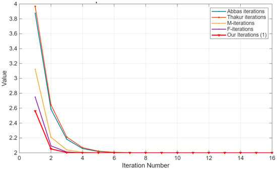
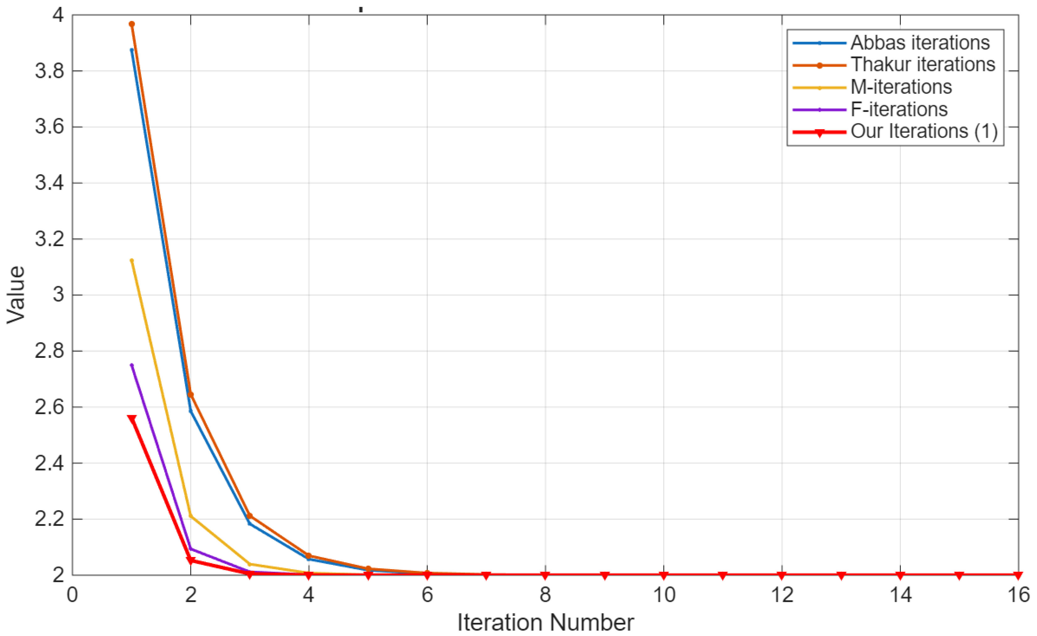
Next, we present an example of numerical computation and show that our iteration scheme enables faster convergence compared to other schemes. We take $Tx={\displaystyle \frac{x}{2}}+1$ with $x_0=8$ and ${\delta }_n={\beta }_n={\nu }_n={\varpi }_n=0.5.$ All the sequences converge to $x^{*}=2$. The comparison in the Table 1 shows that the rate of convergence of our iteration process (1) is faster than other iteration schemes. This fact is also described in Figure 1.

Table 1. Comparison of different iterative schemes.

n	Abbas Iterations	Thakur Iterations	M-Iterations	F-Iterations	Our Iterations (1)
1	3.87500000	3.96875000	3.12500000	2.75000000	2.56250000
2	2.58593750	2.64599609	2.21093750	2.09375000	2.05273438
3	2.18310547	2.21196747	2.03955078	2.01171875	2.00494385
4	2.05722046	2.06955183	2.00741577	2.00146484	2.00046349
5	2.01788139	2.02282169	2.00139046	2.00018311	2.00004345
6	2.00558794	2.00748837	2.00026071	2.00002289	2.00000407
7	2.00174623	2.00245712	2.00004888	2.00000286	2.00000038
8	2.00054570	2.00080624	2.00000917	2.00000036	2.00000004
9	2.00017053	2.00026455	2.00000172	2.00000004	2.00000000
10	2.00005329	2.00008680	2.00000032	2.00000001	2.00000000
11	2.00001665	2.00002848	2.00000006	2.00000000	2.00000000
12	2.00000520	2.00000935	2.00000001	2.00000000	2.00000000
13	2.00000163	2.00000307	2.00000000	2.00000000	2.00000000
14	2.00000051	2.00000101	2.00000000	2.00000000	2.00000000
15	2.00000016	2.00000033	2.00000000	2.00000000	2.00000000
16	2.00000005	2.00000011	2.00000000	2.00000000	2.00000000

Figure 1. Comparison of Different Iteration Schemes.

5. Application

In this section, Theorem 1 is used to demonstrate the existence of a solution for the following integral equation [28]:

$$x\left(\sigma \right)\in f\left(\sigma \right)+{\int }_l^{m}u(\sigma ,\delta )K_1(\delta ,x\left(\delta \right))d\delta .{\int }_l^{m}u(\sigma ,\delta )K_2(\delta ,x\left(\delta \right))d\delta ,$$

(33)

where $\sigma \in [l,m]$, $f:[l,m]\to \mathbb{R}$, $x:[l,m]\times [l,m]\to [0,+\infty )$ and $K_1,K_2:[l,m]\times \mathbb{R}\to \mathbb{R}$ are continuous functions. Let $\Pi =C\left(\right[l,m],\mathbb{R})$ denote the space of all continuous functions on $[l,m]$. Suppose that $d:\Pi \times \Pi ⟶[0,+\infty )$ is defined by $d(x,y)={sup}_{\sigma \in [l,m]}|x\left(\sigma \right)-y\left(\sigma \right)|$ and the function $\mathcal{W}:\Pi \times \Pi \times (0,1)⟶\Pi$ is defined as

$$\mathcal{W}(x,y,\alpha )=\alpha x+(1-\alpha )y.$$

It is well known that $(X,d,\mathcal{W})$ is a complete $CMS$.

Define multi-valued mapping $T:\Pi \to \Pi$ as

$$Tx\left(\sigma \right)=p\left(\sigma \right)\in \Pi :p\left(\sigma \right)=f\left(\sigma \right)+{\int }_l^{m}u(\sigma ,\delta )K_1(\delta ,x\left(\delta \right))d\delta .{\int }_l^{m}u(\sigma ,\delta )K_2(\delta ,x\left(\delta \right))d\delta .$$

Obviously, T is well defined.

Next, we present our result.

Theorem 4.

Assume that the following conditions are satisfied:

(i) 

${\int }_l^m\left|u(\sigma ,\delta )\right|d\delta \le 1$;

(ii) 

$$\begin{gathered} \mathit{for}\mathit{all}p,q\in \Pi ,\mathit{and}{k}_i(\sigma ,x\left(\sigma \right))\in K_i(\sigma ,x\left(\sigma \right))(i=1,2),\mathit{there}\mathit{exists} \\ {k}_i(\sigma ,y\left(\sigma \right))\in K_i(\sigma ,y\left(\sigma \right))\mathit{such}\mathit{that}\hspace{1em}|k_i(\delta ,x\left(\delta \right))-k_i(\delta ,y\left(\delta \right))|\le |x-y|,\hspace{1em}i=1,2. \\ {\int }_l^{m}u(\sigma ,\delta )|k_1(\delta ,y\left(\delta \right))|d\delta +{\int }_l^{m}u(\sigma ,\delta )\left|k_2(\delta ,x\left(\delta \right))\right|d\delta =1 \end{gathered}$$.

Then, the integral Equation (33) has a solution $x\left(\sigma \right)\in \Pi$.

Proof. 

It is sufficient to find a fixed point of T to guarantee a solution for integral Equation (33). Suppose that there exist two continuous mappings $k_1(\delta ,x\left(\delta \right))$ and $k_2(\delta ,x\left(\delta \right))$ such that

$$p\left(\sigma \right)=f\left(\sigma \right)+{\int }_l^{m}u(\sigma ,\delta )K_1(\delta ,x\left(\delta \right))d\delta .{\int }_l^{m}u(\sigma ,\delta )K_2(\delta ,x\left(\delta \right))d\delta .$$

By condition (ii), there exist $k_1(\delta ,x\left(\delta \right))$ and $k_2(\delta ,x\left(\delta \right))$, such that

$$|k_i(\delta ,x\left(\delta \right))-k_i(\delta ,y\left(\delta \right))|\le |x-y|,\hspace{1em}i=1,2.$$

Let

$$q\left(\sigma \right)=f\left(\sigma \right)+{\int }_l^{m}u(\sigma ,\delta )K_1(\delta ,y\left(\delta \right))d\delta .{\int }_l^{m}u(\sigma ,\delta )K_2(\delta ,y\left(\delta \right))d\delta$$

which yields

$$q\left(\sigma \right)\in f\left(\sigma \right)+{\int }_l^{m}u(\sigma ,\delta )K_1(\delta ,y\left(\delta \right))d\delta .{\int }_l^{m}u(\sigma ,\delta )K_2(\delta ,y\left(\delta \right))d\delta .$$

Therefore, $q\in Ty$. Notice that

$$\begin{array}{cc}\hfill d(p,q)& =\underset{\sigma \in [a,b]}{sup}\left|p\left(\sigma \right)-q\left(\sigma \right)\right|\hfill \\ \hfill \hspace{1em}& \le \underset{\sigma \in [a,b]}{sup}|{\int }_l^{m}u(\sigma ,\delta )k_1(\delta ,x\left(\delta \right))d\delta {\int }_l^{m}u(\sigma ,\delta )k_2(\delta ,x\left(\delta \right))d\delta \hfill \\ \hfill \hspace{1em}& -{\int }_l^{m}u(\sigma ,\delta )k_1(\delta ,y\left(\delta \right))d\delta {\int }_l^{m}u(\sigma ,\delta )k_2(\delta ,y\left(\delta \right))d\delta |\hfill \\ \hfill \hspace{1em}& \le \underset{\sigma \in [a,b]}{sup}|{\int }_l^{m}u(\sigma ,\delta )k_1(\delta ,x\left(\delta \right))d\delta {\int }_l^{m}u(\sigma ,\delta )k_2(\delta ,x\left(\delta \right))d\delta \hfill \\ \hfill \hspace{1em}& -{\int }_l^{m}u(\sigma ,\delta )k_1(\delta ,y\left(\delta \right))d\delta {\int }_l^{m}u(\sigma ,\delta )k_2(\delta ,x\left(\delta \right))d\delta |\hfill \\ \hfill \hspace{1em}& +|{\int }_l^{m}u(\sigma ,\delta )k_1(\delta ,y\left(\delta \right))d\delta {\int }_l^{m}u(\sigma ,\delta )k_2(\delta ,x\left(\delta \right))d\delta \hfill \end{array}$$

$$\begin{array}{cc}\hfill \hspace{1em}& -{\int }_l^{m}u(\sigma ,\delta )k_1(\delta ,y\left(\delta \right))d\delta {\int }_l^{m}u(\sigma ,\delta )k_2(\delta ,y\left(\delta \right))d\delta |\hfill \\ \hfill \hspace{1em}& \le \underset{\sigma \in [a,b]}{sup}\left\{{\int }_l^{m}u(\sigma ,\delta )|k_1(\delta ,x\left(\delta \right))-k_1(\delta ,y\left(\delta \right))|d\delta ·{\int }_l^{m}u(\sigma ,\delta )k_2(\delta ,x\left(\delta \right))d\delta \right.\hfill \\ \hfill \hspace{1em}& \hspace{1em}\left.+{\int }_l^{m}u(\sigma ,\delta )k_1(\delta ,y\left(\delta \right))d\delta {\int }_l^{m}u(\sigma ,\delta )|k_2(\delta ,x\left(\delta \right))-k_2(\delta ,y\left(\delta \right))|d\delta \right\}\hfill \\ \hfill \hspace{1em}& \le \underset{\sigma \in [a,b]}{sup}\left\{{\int }_l^{m}u(\sigma ,\delta )|x\left(\delta \right)-y\left(\delta \right)|d\delta ·{\int }_l^{m}u(\sigma ,\delta )k_2(\delta ,x\left(\delta \right))d\delta \right.\hfill \\ \hfill \hspace{1em}& \hspace{1em}\left.+{\int }_l^{m}u(\sigma ,\delta )k_1(\delta ,y\left(\delta \right))d\delta {\int }_l^{m}u(\sigma ,\delta )|x\left(\delta \right)-y\left(\delta \right)|d\delta \right\}\hfill \\ \hfill \hspace{1em}& \le \underset{\sigma \in [a,b]}{sup}|x\left(\sigma \right)-y\left(\sigma \right)|\left({\int }_l^{m}u(\sigma ,\delta )d\delta {\int }_l^{m}u(\sigma ,\delta )k_2(\delta ,x\left(\delta \right))d\delta \right)\hfill \\ \hfill \hspace{1em}& +\underset{\sigma \in [a,b]}{sup}|x\left(\sigma \right)-y\left(\sigma \right)|\left({\int }_l^{m}u(\sigma ,\delta )k_1(\delta ,y\left(\delta \right))d\delta {\int }_l^{m}u(\sigma ,\delta )d\delta \right)\hfill \\ \hfill \hspace{1em}& \le \underset{\sigma \in [a,b]}{sup}|x\left(\sigma \right)-y\left(\sigma \right)|{\int }_l^{m}u(\sigma ,\delta )d\delta ({\int }_l^{m}u(\sigma ,\delta )k_2(\delta ,x\left(\delta \right))d\delta \hfill \\ \hfill \hspace{1em}& +{\int }_l^{m}u(\sigma ,\delta )k_1(\delta ,y\left(\delta \right))d\delta ).\hfill \end{array}$$

By conditions (i) and (ii), we obtain

$$d(p,q)\le d(x,y)$$

By interchanging the role of x and y, we can conclude that $H(Tx,Ty)\le d(x,y)$. Hence, by Theorem 1, we get that the integral Equation (33) has a solution $x\left(\sigma \right)$ satisfying ${lim}_{n\to +\infty }{x}_n\left(\sigma \right)=x\left(\sigma \right)$ for the sequence $\left\{x_n\right\}$ generated by (1). □

6. Conclusions

In this paper, we demonstrate the derivation of approximate fixed point results for generalized $\alpha$-non-expansive multi-valued mappings through a four-step iteration scheme. We extend the results of Iqbal et al. [25] from a Banach space to a $CMS$. An example of a generalized $\alpha$-non-expansive multi-valued mapping is presented. Through the included table and graph, we show that our iteration scheme enables faster convergence than other well-known schemes. Moreover, an example is given to demonstrate the application of Theorem 1 to solve an integral equation.

References

- Markin, J. A fixed point theorem for set valued mappings. Bull. Am. Math. Soc. 1968, 74, 639–640. [Google Scholar] [CrossRef] [Scilit]
- Nadler, S.B., Jr. Multi-valued contraction mappings. Pac. J. Math. 1969, 30, 475–488. [Google Scholar] [CrossRef] [Scilit]
- Azam, A.; Rashid, M.; Kalsoom, A.; Ali, F. Fixed-point convergence of multi-valued non-expansive mappings with applications. Axioms 2023, 12, 1020. [Google Scholar] [CrossRef] [Scilit]
- Shahzad, N.; Zegeye, H. On Mann and Ishikawa iteration schemes for multi-valued maps in Banach space. Nonlinear Anal. 2009, 71, 838–844. [Google Scholar] [CrossRef] [Scilit]
- Berinde, V. A projection-type implicit algorithm for finding a common solution for fixed point problems and variational inequality problems. Mathematics 2024, 12, 3187. [Google Scholar] [CrossRef] [Scilit]
- Pant, R.; Shukla, R. Approximating fixed points of generalized α-non-expansive mapping in Banach space. Numer. Funct. Anal. Optim. 2017, 38, 248–266. [Google Scholar] [CrossRef] [Scilit]
- Berinde, V. Approximating fixed points of demicontractive mappings via the quasi-non-expansive case. Carpathian J. Math. 2023, 39, 73–85. [Google Scholar] [CrossRef] [Scilit]
- Achtoun, Y.; Radenović, S.; Tahiri, I.; Sefian, M.L. The nonlinear contraction in probabilistic cone b-metric spaces with application to integral equation. Nonlinear Anal. Model. Control 2024, 29, 658–669. [Google Scholar] [CrossRef] [Scilit]
- García-Falset, J.; Llorens-Fuster, E.; Moreno Gaávez, E. Fixed point theory for multi-valued generalized non-expansive mappings. Appl. Anal. Discr. Math. 2012, 1, 265–286. [Google Scholar] [CrossRef] [Scilit]
- Ahmad, J.; Kallel, I.A.; Aloqaily, A.; Mlaiki, N. On multi-valued generalized α-non-expansive mappings and an application to two-point BVPs. AIMS Math. 2025, 10, 403–419. [Google Scholar] [CrossRef] [Scilit]
- Nawaz, S.; Rafique, K.; Batool, A.; Mahmood, Z.; Muhammad, T. Fixed point approximation of multi-valued non-expansive mappings in uniformly convex Banach spaces via AR-iteration. Mod. Phys. Lett. B 2025, 39, 2450495. [Google Scholar] [CrossRef] [Scilit]
- Hussain, T.; Khan, A.R.; Riaz, K.; Alamri, H. Approximating common fixed points of non-expansive type multi-valued mappings in convex metric space. AIMS Math. 2025, 10, 30053–30067. [Google Scholar] [CrossRef] [Scilit]
- García-Falset, J.; Llorens-Fuster, E.; Suzuki, T. Fixed point theory for a class of generalized non-expansive mappings. J. Math. Anal. Appl. 2011, 375, 185–195. [Google Scholar] [CrossRef] [Scilit]
- Abbas, M.; Nazir, T. Some new faster iteration process applied to constrained minimization and feasibility problems. Mat. Vesn. 2014, 66, 223–234. [Google Scholar]
- Thakur, D.; Thakur, B.S.; Postolache, M. New iteration scheme for numerical reckoning fixed points of non-expansive mappings. J. Inequal. Appl. 2014, 2014, 328. [Google Scholar] [CrossRef] [Scilit]
- Ullah, K.; Ahmad, J.; Khan, M.S.; Muhammad, N. Convergence results of a faster iterative scheme including multi-valued mappings in Banach spaces. Filomat 2021, 35, 1359–1368. [Google Scholar] [CrossRef] [Scilit]
- Ali, J.; Jubair, M.; Ali, F. Stability and convergence of F iterative scheme with an application to the fractional differential equation. Eng. Comput. 2022, 38, 693–702. [Google Scholar] [CrossRef] [Scilit]
- Garodia, C.; Uddin, I. A new fixed point algorithm for finding the solution of a delay differential equation. AIMS Math. 2020, 5, 3182–3200. [Google Scholar] [CrossRef] [Scilit]
- Takahashi, W. A convexity in metric space and non-expansive mappings. Kodai Math. Sem. Rep. 1970, 22, 142–149. [Google Scholar] [CrossRef] [Scilit]
- Abbas, M. Common fixed point results with applications in convex metric space. Fasc. Math. 2008, 39, 5–15. [Google Scholar]
- Fukhar-Ud-Din, H. Existence and approximation of fixed points in convex metric spaces. Carpathian J. Math. 2014, 30, 175–185. [Google Scholar] [CrossRef] [Scilit]
- Kirk, W.A.; Panyanak, B. A concept of convergence in geodesic spaces. Nonlinear Anal. 2008, 68, 3689–3696. [Google Scholar] [CrossRef] [Scilit]
- Suzuki, T. Fixed point theorems and convergence theorems for some generalized non-expansive mappings. J. Math. Anal. Appl. 2008, 340, 1088–1095. [Google Scholar] [CrossRef] [Scilit]
- Abkar, A.; Eslamian, M. A fixed point theorem for generalized non-expansive multi-valued mappings. Fixed Point Theory 2011, 12, 241–246. [Google Scholar]
- Iqbal, H.; Abbas, M.; Husnine, S.M. Existence and approximation of fixed points of multi-valued generalized α-nonexpansive mappings in Banach spaces. Numer. Algorithms 2020, 85, 1029–1049. [Google Scholar] [CrossRef] [Scilit]
- Fukhar-ud-Din, H. One step iterative scheme for a pair of non-expansive mappings in a convex metric space. Hacet. J. Math. Stat. 2015, 44, 1023–1031. [Google Scholar]
- Aistleitner, C.; Brauchart, J.S.; Dick, J. Point sets on the sphere with small spherical cap discrepancy. Discret. Comput. Geom. 2012, 48, 990–1024. [Google Scholar]
- Ji, D.; Li, C.; Cui, Y. Fixed point theorems for Mann’s iteration scheme in convex Gb-metric spaces with an application. Axioms 2023, 12, 108. [Google Scholar] [CrossRef] [Scilit]
Disclaimer/Publisher’s Note: The statements, opinions and data contained in all publications are solely those of the individual author(s) and contributor(s) and not of MDPI and/or the editor(s). MDPI and/or the editor(s) disclaim responsibility for any injury to people or property resulting from any ideas, methods, instructions or products referred to in the content. |
© 2026 by the authors. Licensee MDPI, Basel, Switzerland. This article is an open access article distributed under the terms and conditions of the Creative Commons Attribution (CC BY) license.