


Abstract
In this work, we revisit the two-step Jarratt method from the perspective of numerical stability. While high-order iterative schemes are often examined in terms of convergence rate and computational efficiency, their backward stability properties have received comparatively less attention. We begin by establishing the method’s strong consistency. Next, we provide a quantitative backward stability assessment within the standard floating-point arithmetic framework, deriving explicit perturbation bounds that show that the iteration errors remain proportional to machine precision. To support the theoretical findings, we present numerical experiments—including tests under finite-precision perturbations—as well as Python implementations and visualizations of the numerical examples. The results illustrate that the two-step Jarratt method not only achieves a high convergence order but also remains numerically robust for well-conditioned nonlinear systems.
Keywords:
nonlinear equations; iterative methods; Jarratt method; consistency; backward stability; convergence MSC:
65H10
1. Introduction
High-order iterative methods for solving nonlinear systems have been extensively studied from the viewpoint of convergence order and efficiency [1,2,3,4,5,6,7,8,9,10,11,12,13,14,15,16,17,18,19,20,21,22,23,24,25,26,27,28,29,30]. However, numerical stability—particularly backward stability—has received comparatively less attention [31,32].
While Newton’s method has been analyzed from a backward error perspective (Wozniakowski [33] and Tisseur [34]), similar stability investigations for multipoint high-order methods remain limited.
In particular, despite the widespread development of Jarratt-type methods for nonlinear systems, a quantitative backward stability analysis for the classical two-step Jarratt method has not been explicitly established. More recently, the discrete dynamical systems approach has provided valuable tools for analyzing the behavior of iterative methods. Developments in this area include the extension of classical dynamics to vector-valued rational functions, leading to the identification of phenomena such as strange attractors and periodic cycles [6,8]. Additionally, the use of isonormal surfaces has been proposed to detect regions of instability and chaos in parameter spaces [9]. Fourth-order Jacobian-free methods have also shown promising stability and robustness over wide parameter intervals, with divergence occurring only in isolated cases [10].
Numerical methods are typically divided into two classes [31,32]: direct algorithms that compute exact solutions in a bounded number of steps and approximation techniques that iteratively solve modified problems to approximate the original problem . Gaussian elimination exemplifies the former, while the latter is essential for problems where exact solutions are infeasible. Consistency assesses how well approximates as k grows, but practical relevance lies in the convergence of the computed solution to the true value . Importantly, convergence depends not only on consistency but also on the numerical stability of the procedure. Under reasonable assumptions, consistency and stability together ensure convergence [32,35].
The objective of this paper is to carry out consistency and backward stability analysis of the two-step Jarratt method introduced in [11] for solving systems of nonlinear equations [13,14]. In other words, the main contributions of this paper are:
- A strengthened consistency analysis including local truncation structure.
- A quantitative backward stability result with conditioning-dependent bounds.
- An explicit discussion of the role of Jacobian conditioning.
- Numerical validation under finite-precision perturbations.
Let and be an equation with a solution such that the Jacobian matrix is nonsingular. The optimal two-step Jarratt method, originally developed for solving nonlinear scalar equations, was extended by Ren et al. [13] to systems of nonlinear equations as follows:
where and are vectors in , is an initial guess, and denotes the Jacobian matrix.
Theorem 1
([13]). The two-step iterative Jarratt method (1) possesses local order of convergence at least four with the following error equation:
where , , .
The remainder of this paper is organized as follows: In Section 2, we review some fundamental concepts required for the subsequent analysis. Section 3 is devoted to the consistency of the Jarratt method (1) for solving systems of nonlinear equations. Section 4 focuses on the backward stability of the method. The manuscript ends with some conclusions in Section 5.
2. Mathematical Preliminaries
To establish the theoretical basis for the analysis that follows, we first review key mathematical concepts required for subsequent developments. In particular, we adopt the framework introduced by Wozniakowski [33] and further elaborated in [34], which provides a rigorous foundation for analyzing the data vectors, condition numbers and numerical stability of the iterative methods in high-dimensional settings. The notation and analytical tools developed in these works will be employed throughout the remainder of this paper.
We consider the numerical solution of equation
where is in general a nonlinear function
We want to solve (3) by iteration, say Jarratt’s method (1). Let be a sufficiently close approximation of the solution , . We assume that depends parametrically on a vector , called a data vector,
and instead of the exact value we only have the computed value in t digit floating-point binary arithmetic [36]. We consider the following definition for well-posedness problems [31].
Definition 1.
Let
be continuously differentiable in a neighborhood of . Assume:
- ;
- is nonsingular;
- is locally Lipschitz continuous;
- The Jacobian is continuous near .
Then the nonlinear system is locally well-posed in the sense of Hadamard.
By the Implicit Function Theorem [1], the nonsingularity of ensures local uniqueness. Continuity implies stability under perturbations of the data. Hence, the solution depends continuously on the data vector [31]
3. Numerical Consistency of the Jarratt Iterative Method
In this section, we demonstrate that the Jarratt iterative method (1) for solving systems of nonlinear equations is a numerically consistent method. In fact, consistency states that the iterative Jarratt method performs correctly when the input and output data are exact. However, in the error analysis of this method, two types of errors must be considered: first, the discretization error, which is inherent to the numerical method itself and typically appears as a truncation error, and second, the implementation error, which arises when the method is executed on a computer or numerical algorithm, which may include rounding errors due to finite-precision arithmetic [32].
The concept of consistency is related to the discretization error and evaluates how well the numerical method approximates the original mathematical model. Therefore, consistency is not concerned with rounding errors or other algorithmic implementation errors.
In Partial Differential Equation (PDE) discretization, consistency is linked to the vanishing of a local truncation error with respect to a mesh parameter. However, in fixed-point iterative solvers, there is no external discretization parameter. Instead, consistency means that the discrete operator preserves the exact solution when exact arithmetic is assumed. In other words, the exact solution must be an invariant point of the iteration operator [29]. For multipoint methods such as the two-step Jarratt scheme, this verification is necessarily structural: one must show that substituting the exact solution into each stage of the method leaves it unchanged. This is precisely what strong consistency requires.
Definition 2.
Let be a valid input for the original problem (4), . We say that the discrete problem is consistent if or
is defined, as its output corresponds to the exact solution of problem (3) for the input .
Furthermore, the method is said to be strongly consistent if this property holds not only for a specific k but for all k.
Theorem 2.
Let be a sufficiently smooth function, and is nonsingular. Then the iterative Jarratt method (1) is strongly consistent.
Proof.
To prove this, we show that both steps of Method (1) are consistent. For the first step, we can write
Considering that is a simple root and , is nonsingular and (5), then
This implies that the first step of the method is consistent. Similarly, with slight modifications, the second step can be written as
Now, based on the assumptions and using (5) and considering (7), we have
This shows that the second step of the Jarratt method is also consistent, and thus the proof is complete. □
Consistency of a numerical method ensures that the numerical approximation accurately reflects the original equation. It guarantees that the discretization error decreases as the step size becomes smaller. In error analysis, consistency is a fundamental requirement for the convergence of the method. Without consistency, the numerical solution may fail to approach the exact solution even as the step size tends to zero.
4. Backward Stability of the Jarratt Iterative Method
Equation (1) provides the discrete properties of the iterative Jarratt method, which we have shown to be consistent. We now redefine it as follows:
Let us remark that the formula is written in a new form to avoid confusion with the computed value , which includes the effect of rounding errors.
However, in practical implementation on a computer, in addition to the discretization error, rounding errors may also occur. As a result, instead of the ideal relation (8), we actually have
where actually represents the difference between the value computed by the discretization method and the one obtained by its computer implementation, which includes the rounding error. In other words
quantifies the deviation from the exact value in a single update cycle. In the following, we present the backward stability of the Jarratt iterative method (1). Backward error analysis plays a central role in the assessment of numerical algorithms. The key question it addresses is “For which (slightly perturbed) input data is the computed solution the exact solution?” In this type of analysis, the objective is to determine an upper bound for the perturbation in the input data, that is, to find a bound for the data perturbation vector such that . An algorithm is said to be backward stable if it produces a small backward error; that is, the computed solution coincides with the exact solution of a nearby problem. We now present a formal definition of backward stability for iterative methods [33].
Definition 3.
An iteration φ is called backward stable if there exist and such that
and
where and are constants that only depend on the size of the problem and denotes the machine precision in t digit floating-point binary arithmetic.
Backward stability implies that a computed solution , for sufficiently large k, which has been slightly perturbed, corresponds to an almost exact solution of a nearby (i.e., slightly perturbed) problem [6,14].
Theorem 3.
Assume that the Jarratt iterative method is described by (1). If and there exist and for large k such that
where and stand for Jacobian matrices with respect to and , respectively, then it is backward stable.
Proof.
According to Definition 2, we need to find and of order such that
Taking into account (9) and (12), Taylor series expansion for (12) around and implies
where ,and . Notice that if we let , then (13) yields
Considering (9), and according to (11), we can write
Hence
Substituting (15) into (14) yields
Finally, it is enough to consider. □
In order to make the backward stability result constructive rather than merely formal, we explicitly analyze the propagation of floating-point errors under the standard model of finite-precision arithmetic [31,32,33]. We assume that each arithmetic operation satisfies
where denotes the machine precision.
Recall that one ideal Jarratt iteration can be written as
where
In floating-point arithmetic, the computed iterate satisfies
where represents the accumulated rounding error. Each of the following operations introduces perturbations:
- Evaluation of ;
- Evaluation of and ;
- Matrix inversion and ;
- Matrix–matrix and matrix–vector multiplications.
Using standard backward error results for matrix multiplication and inversion (see [31]), we have
and
where
Collecting all perturbations introduced during one iteration, we obtain the bound
for some moderate constant depending on the number of arithmetic operations per step.
Near the solution , since and remains nonsingular, we deduce
To establish constructive backward stability, define the perturbation
Then, by Taylor expansion,
and the perturbation satisfies
Therefore, the two-step Jarratt method is backward stable in a constructive sense:the computed iterate coincides with the exact solution of a nearby nonlinear problem whose perturbation is bounded by . The constant depends only on bounds of , the Lipschitz constant of , and the problem dimension n, but is independent of k.
Theorem 4
(Local convergence radius estimate). Assume that
Then the Jarratt iteration (1) converges to if the initial guess satisfies
The above result places the two-step Jarratt method within the classical framework of backward error analysis as developed in modern numerical linear algebra. In particular, following the philosophy articulated in Accuracy and Stability of Numerical Algorithms by Nicholas J. Higham [31], an algorithm is said to be backward stable if the computed result is the exact solution of a nearby problem whose perturbation is small relative to machine precision.
Our analysis shows that, under standard floating-point arithmetic, the computed iterate satisfies
which implies that the numerical sequence coincides with the exact sequence of a perturbed nonlinear system
Thus, the perturbations are proportional to machine precision and independent of the iteration index in a neighborhood of the solution. This establishes backward stability in the classical numerical analysis sense, rather than in a merely formal or existential sense.
Based on the results established in the above theorems and in light of the fundamental theorem in numerical analysis [37,38], we conclude the following result.
Corollary 1.
Let be a sufficiently smooth function, and let be nonsingular. Suppose is close enough to . If the problem is well-posed and the sequence generated by iterative Jarratt method (1) is consistent and backward stable, then it is also convergent.
5. Numerical Experiments
This section provides numerical evidence supporting the theoretical analysis developed in Section 3 and Section 4. In particular, we examine:
- local convergence behavior;
- sensitivity under Jacobian perturbations of order ;
- comparison with Newton’s method.
All computations were performed in double-precision arithmetic (IEEE 754) in Python (see codes in Appendix A). The stopping criterion was
or a maximum number of iterations .
To validate the backward stability claim, we also considered a perturbed-Jacobian scenario in which the Jacobian matrix is subject to relative componentwise perturbations of the order of machine precision:
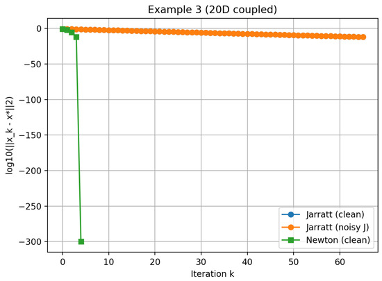
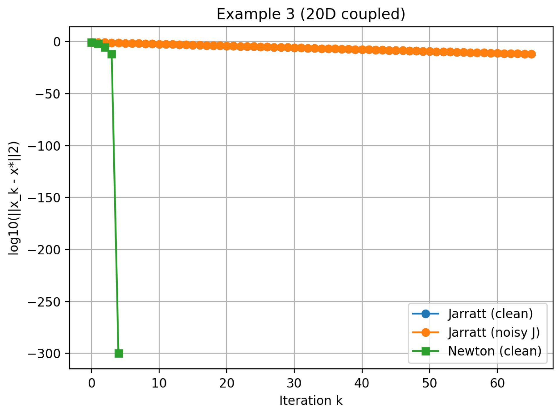
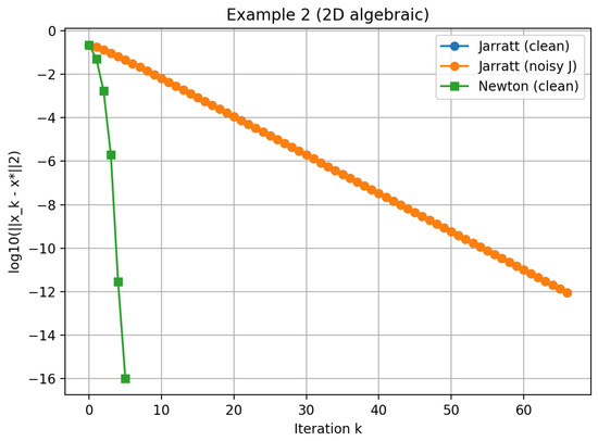
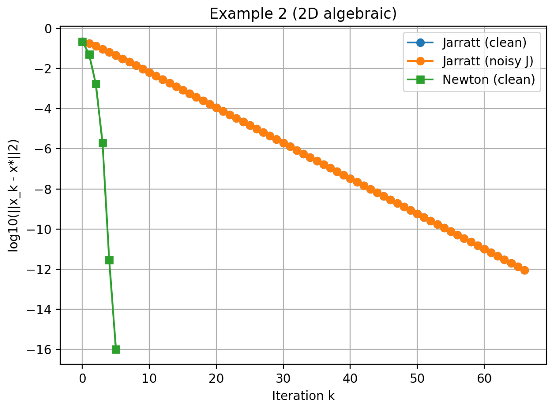
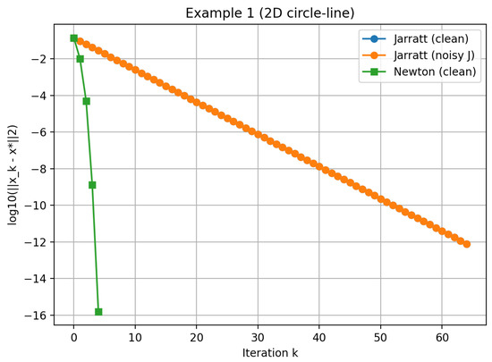
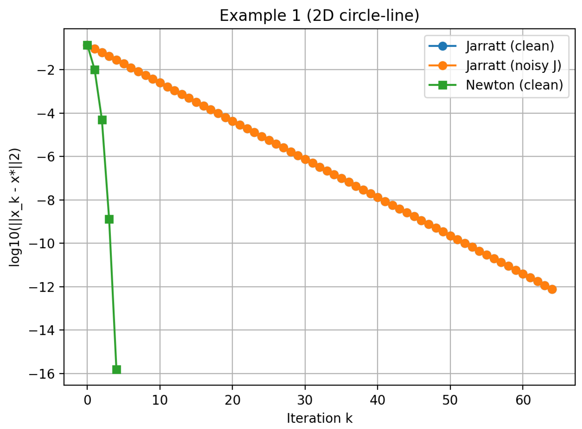
In Table 1 and Figure 1, Figure 2 and Figure 3, we compare the two-step Jarratt method with the classical Newton method. For each test problem we report: number of iterations, final error , and final residual . In addition, we plot convergence curves (logarithm of the error versus iteration index).
Table 1.
Numerical comparison between the Newton and two-step Jarratt methods (clean vs. noisy Jacobian).
Figure 1.
Convergence curves (log10 of versus iteration) for Example 1, comparing the Newton and two-step Jarratt methods under clean and noisy Jacobian scenarios.
Figure 2.
Convergence curves (log10 of versus iteration) for Example 2, comparing the Newton and two-step Jarratt methods under clean and noisy Jacobian scenarios.
Figure 3.
Convergence curves (log10 of versus iteration) for Example 3, comparing the Newton and two-step Jarratt methods under clean and noisy Jacobian scenarios.
Test Problems
- Example 1 (2D circle-line):
- Example 2 (2D algebraic):
- Example 3 (20D coupled):
Let . Define
with solution .
6. Conclusions
In this work, we have revisited the two-step Jarratt method from the viewpoint of numerical stability. The main results can be summarized as follows. We established strong consistency and analyzed the local truncation structure, confirming fourth-order behavior. We derived a quantitative backward stability estimate showing that perturbations are bounded proportionally to the condition number of the Jacobian. We clarified the relationship between stability and conditioning. Numerical experiments under finite-precision arithmetic confirmed the theoretical predictions. These results demonstrate that the two-step Jarratt method is not only efficient in terms of convergence order but also numerically reliable for well-conditioned nonlinear systems. Future research may include stability analysis of higher-order Jarratt-type schemes, investigation of inexact Jacobian evaluations, and extension to large-scale or structured nonlinear systems.
Author Contributions
Conceptualization, T.L.; Validation, A.C.; Formal analysis, J.R.T.; Investigation, V.R.; Writing—original draft, V.R.; Writing—review & editing, A.C. and J.R.T.; Supervision, T.L. All authors have read and agreed to the published version of the manuscript.
Funding
This research received no external funding.
Data Availability Statement
No new data were created or analyzed in this study. Therefore, data sharing is not applicable to this article.
Acknowledgments
The authors would like to sincerely thank the anonymous reviewers for their careful reading of the manuscript and for their constructive comments, which have significantly improved the clarity and quality of this work.
Conflicts of Interest
No potential conflict of interest was reported by the authors.
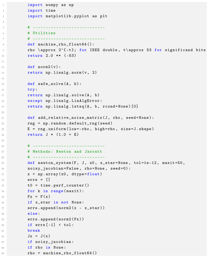
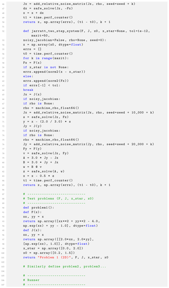
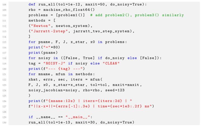
Appendix A. Python Code Example: Newton and Jarratt Methods for Nonlinear Systems
References
- Ortega, J.M.; Rheinboldt, W.G. Iterative Solution of Nonlinear Equations in Several Variable; Academic Press: New York, NY, USA, 1970. [Google Scholar]
- Traub, J.F. Iterative Methods for the Solution of Equation; Prentice-Hall: Englewood Cliff, NJ, USA, 1964. [Google Scholar]
- Yu, J.; Wang, X. A single parameter fourth-order Jarratt type iterative method for solving nonlinear systems. AIMS Math. 2025, 10, 7847–7863. [Google Scholar] [CrossRef] [Scilit]
- Cordero, A.; Lotfi, T.; Mahdiani, K.; Torregrosa, J.R. A stable family with high order of convergence for solving nonlinear equation. Appl. Math. Comput. 2015, 254, 240–251. [Google Scholar] [CrossRef] [Scilit]
- Bakhtiari, P.; Cordero, A.; Lotfi, T.; Mahdiani, K.; Torregrosa, J.R. Widening basins of attraction of optimal iterative method. Nonlinear Dyn. 2017, 87, 913–938. [Google Scholar] [CrossRef] [Scilit]
- Cordero, A.; Soleymani, F.; Torregrosa, J.R. Dynamical analysis of iterative methods for nonlinear systems or how to deal with the dimension. Appl. Math. Comput. 2014, 244, 398–412. [Google Scholar] [CrossRef] [Scilit]
- Moccari, M.; Lotfi, T. On a two-step optimal Steffensen-type method: Relaxed local and semi-local convergence analysis and dynamical stability. J. Math. Anal. Appl. 2018, 468, 240–269. [Google Scholar] [CrossRef] [Scilit]
- Asghari, S.; Lotfi, T.; Moccari, M. Efficient conformable iterative approaches for solving nonlinear equations via comprehensive dynamical stability analysis. J. Anal. 2025, 33, 2061–2080. [Google Scholar] [CrossRef] [Scilit]
- Capdevila, R.R.; Cordero, A.; Torregrosa, J.R. Isonormal surfaces: A new tool for the multidimensional dynamical analysis of iterative methods for solving nonlinear system. Math. Methods Appl. Sci. 2022, 45, 3360–3375. [Google Scholar] [CrossRef] [Scilit]
- Cordero, A.; Jordan, C.; Sanabria-Codesal, E.; Torregrosa, J.R. Solving nonlinear vectorial problems with a stable class of Jacobian-free iterative processes. J. Appl. Math. Comput. 2024, 70, 5023–5048. [Google Scholar] [CrossRef] [Scilit]
- Jarratt, P. Some fourth order multipoint iterative methods for solving equations. Math. Comput. 1966, 20, 434–437. [Google Scholar] [CrossRef]
- Chun, C. Some improvements of Jarratt’s method with sixth-order convergence. Appl. Math. Comput. 2007, 190, 1432–1437. [Google Scholar] [CrossRef] [Scilit]
- Ren, H.; Wu, Q.; Bi, W. New variants of Jarratt’s methods with six-order convergence. Numer. Algorithms 2009, 52, 585–603. [Google Scholar] [CrossRef] [Scilit]
- Cordero, A.; Hueso, J.L.; Martinez, E.; Torregrosa, J.R. A Modified Newton-Jarratt’s composition. Numer. Algorithms 2010, 99, 55–87. [Google Scholar] [CrossRef] [Scilit]
- Behl, R.; Kanwar, V.; Sharma, K.K. Optimal equi-scaled families of Jarratt’s metho. Int. J. Comput. Math. 2013, 90, 408–422. [Google Scholar]
- Sharma, J.R.; Arora, H. Efficient Jarratt-like methods for solving systems of nonlinear equation. Calcolo 2014, 51, 193–210. [Google Scholar] [CrossRef] [Scilit]
- Lotfi, T.; Bakhtiari, P.; Cordero, A.; Mahdiani, K.; Torregrosa, J.R. Some new efficient multipoint iterative methods for solving nonlinear systems of equation. Int. J. Comput. Math. 2015, 92, 1921–1934. [Google Scholar] [CrossRef] [Scilit]
- Ahmad, F.; Tohidi, E.; Ullah, M.Z.; Carrasco, J.A. Higher order multi-step Jarratt-like method for solving systems of nonlinear equations: Application to PDEs and ODE. Comput. Math. Appl. 2015, 70, 624–636. [Google Scholar] [CrossRef] [Scilit]
- Chun, C.; Neta, B. Developing high order methods for the solution of systems of nonlinear equation. Appl. Math. Comput. 2019, 342, 178–190. [Google Scholar] [CrossRef] [Scilit]
- Zhanlav, T.; Otgondorj, K. Higher order Jarratt-like iterations for solving systems of nonlinear equation. Appl. Math. Comput. 2021, 395, 125849. [Google Scholar] [CrossRef] [Scilit]
- Argyros, I.K.; Sharma, D.; Argyros, C.I.; Parhi, S.K.; Sunanda, S.K.; Argyros, M.I. Extended three step sixth order Jarratt-like methods under generalized conditions for nonlinear equation. Arab. J. Math. 2022, 11, 443–457. [Google Scholar] [CrossRef] [Scilit]
- Özbana, A.Y.; Kaya, B. A new family of optimal fourth-order iterative methods for nonlinea requation. Results Control. Optim. 2022, 8, 100157. [Google Scholar] [CrossRef] [Scilit]
- Sharma, K.R.; Kumar, S. A class of accurate Newton-Jarratt-like methods with applications to nonlinear model. Comput. Appl. Math. 2022, 41, 46. [Google Scholar] [CrossRef] [Scilit]
- Saheya, B.; Zhanlav, T.; Mijiddorj, R. A novel families of higher-order multistep iterative methods for solving nonlinear system. Math. Methods Appl. Sci. 2025, 48, 8260–8273. [Google Scholar] [CrossRef] [Scilit]
- George, S.; Kunnarath, A.; Sadananda, R.; Jidesh, P.; Argyros, I.K. On obtaining order of convergence of Jarratt-like method without using Taylor series expansion. Comput. Appl. Math. 2024, 43, 246. [Google Scholar] [CrossRef] [Scilit]
- Singh, H.; Sharma, J.R. A fractional Traub-Steffensen-type method for solving nonlinear equation. Numer. Algorithms 2024, 95, 1103–1126. [Google Scholar] [CrossRef] [Scilit]
- Singh, H.; Sharma, J.R. A two-point Newton-like method of optimal fourth order convergence for systems of nonlinear equation. J. Complex. 2025, 86, 101907. [Google Scholar] [CrossRef] [Scilit]
- Sharma, H.; Behl, R.; Kansal, M.K.; Ramos, H. A robust iterative family for multiple roots of nonlinear equations: Enhancing accuracy and handling critical point. J. Comput. Appl. Math. 2024, 444, 115795. [Google Scholar] [CrossRef] [Scilit]
- Chang, C.W.; Qureshi, S.; Argyros, I.K.; Chicharro, F.I.; Soomro, A.A. A modified two-step optimal iterative method for solving nonlinear models in one and higher dimension. Math. Comput. Simul. 2025, 229, 448–467. [Google Scholar] [CrossRef] [Scilit]
- Junjua, M.; Kumar, S.; Ali, R. A robust family of optimal fourth-order iteration schemes for multiple roots with application. J. Comput. Appl. Math. 2026, 471, 116758. [Google Scholar] [CrossRef] [Scilit]
- Higham, N.J. Accuracy and Stability of Numerical Algorithm, 2nd ed.; SIAM: Philadelphia, PA, USA, 2002. [Google Scholar]
- Hackbusch, W. The Concept of Stability in Numerical Method; Springer: Berlin/Heidelberg, Germany, 2014. [Google Scholar]
- Wozniakowski, H. Numerical stability for solving nonlinear equations. Numer. Math. 1976, 27, 373–390. [Google Scholar] [CrossRef] [Scilit]
- Tisseur, F. Newton’s method in floating point arithmetic and iterative refinement of generalized eigenvalue problems. SIAM J. Matrix Anal. Appl. 2001, 22, 1038–1057. [Google Scholar] [CrossRef] [Scilit]
- Quarteroni, A.; Sacco, R.; Saleri, F. Numerical Mathematic; Springer: Berlin/Heidelberg, Germany, 2000. [Google Scholar]
- Kahan, W. A Survey of Error Analysis; IFIP Congress: Laxenburg, Austria, 1971; Volume I, pp. 220–226. [Google Scholar]
- Lax, P. Numerical solution partial differential equation. Am. Math. Mon. 1965, 72, 74–84. [Google Scholar] [CrossRef] [Scilit]
- Morozov, V. Methods for Solving Incorrectly Posed Problem; Springer: Berlin/Heidelberg, Germany, 1984. [Google Scholar]

Disclaimer/Publisher’s Note: The statements, opinions and data contained in all publications are solely those of the individual author(s) and contributor(s) and not of MDPI and/or the editor(s). MDPI and/or the editor(s) disclaim responsibility for any injury to people or property resulting from any ideas, methods, instructions or products referred to in the content. |
© 2026 by the authors. Licensee MDPI, Basel, Switzerland. This article is an open access article distributed under the terms and conditions of the Creative Commons Attribution (CC BY) license.