


Abstract
This study analyzes network coherence in two-layer and three-layer networks with positive and negative inter-layer correlation patterns. Using algebraic graph theory, we construct the Laplacian matrices for different correlated graph structures and compute their Laplacian spectra. The impact of correlation patterns on network coherence is investigated for two-layer and three-layer structures, and numerical evaluations are performed. The results show that negative-correlation patterns yield better network coherence than positive ones. This work provides fundamental insights into the structural robustness of layered networks and offers theoretical guidance for the design of robust networked systems.
Keywords:
layered networks; network coherence; Laplacian spectrum; structural robustness; correlation patterns MSC:
93B60; 93D50
1. Introduction
Many complex systems in real life, such as neural networks and information networks, can be described by complex networks. With the deepening of research, this field has made much progress in areas such as network synchronization and propagation [1,2,3,4,5,6,7], key node identification [8], weighted networks [9], high-order interaction network modeling [10], and consensus and robustness [11]. In practical systems, nodes between multiple networks often have connections, while it is difficult for traditional single-layer network models to describe such inter-layer relationships. To this end, researchers have introduced the concept of multilayer networks and have achieved a series of results: for example, Wu et al. [12] analyzed double-layer chain networks with two inter-layer edges and obtained the optimal edge positions for synchronization capability; Wei et al. [13] studied the effects of network scale, intra-layer coupling strength, and positive and negative inter-layer correlations on the synchronization capability of double-layer networks, finding that negative-correlation networks have better synchronizability; Zhu et al. [14] explored the relationship between the synchronizability of multilayer windmill networks and parameters such as network scale, coupling strength, and number of layers.
Noise is ubiquitous in practical systems and affects network dynamics. To measure the degree of consensus among network nodes under noise interference, researchers proposed the concept of network coherence, which is defined as the deviation of node states from the network average state. Patterson and Bamieh [15] proved that under the norm, network coherence is completely determined by the Laplacian spectrum. In the standard framework, disturbances are modeled as Gaussian white noise, which represents a persistent stochastic excitation and is widely adopted because it leads to tractable analytical expressions for the steady-state variance of the system [15,16]. This approach provides a fundamental benchmark for understanding consensus performance under broad-band noise. While our analysis assumes homogeneous coupling and Gaussian noise—common simplifications that enable closed-form spectral solutions—real-world systems may exhibit heterogeneous interactions and colored noise; extending the framework to accommodate such complexities is an important direction for future work. Based on this conclusion, Huang et al. [17] calculated the Laplacian spectra of four types of double-layer multi-star networks and compared their coherence; Gao et al. [18] performed numerical simulation analysis on the first-order coherence of three types of symmetric star networks.
In recent years, spectral methods based on Laplacian eigenvalues have become an important means to quantify consensus performance [15,19]. Although traditional single-layer network models are valuable, it is difficult to use them to describe the complex mechanisms of multilayer coupling in practical systems [20,21]. Layered networks provide a more appropriate framework for describing real systems by explicitly introducing inter-layer coupling [22,23], and related research covers multiplex networks [20], multilayer variable coupling networks [14], and double-layer chain networks [12], etc. In these networks, the inter-layer correlation pattern (positive, negative, or mixed correlation) will significantly affect their synchronization capability, robustness, coherence, and other properties [13,24]. Although the coherence analysis of single-layer networks is relatively mature [25,26,27], the coherence characteristics of layered networks under different correlation patterns still need to be explored in depth.
The principles of layered correlation networks extend to engineered systems. In wireless sensor networks, a two-tier architecture with negative correlation balances energy consumption and interference resilience [28,29]. In heterogeneous multi-robot formations, negatively correlated leader–follower dynamics enhance formation stability under communication noise [30,31]. Multilayer structures also influence other dynamical processes, such as epidemic spread, where cross-layer preventive information affects the final outbreak size [32].
Network coherence, as a key indicator to measure consensus performance under random disturbances, includes first-order coherence () and second-order coherence () [15,16]. Among them, reflects the steady-state variance of state deviation from consensus, and characterizes the system’s response characteristics to noise of different frequencies. Both depend on the eigenvalue distribution of the Laplacian matrix, and smaller values mean better consensus performance [33,34]. Since the foundational work of Patterson and Bamieh [15], coherence research has been extended to various network structures: Sun et al. [27] gave analytical expressions for symmetric and asymmetric ring networks; Liu et al. [35] derived coherence formulas for balanced networks; recent studies also explored the coherence dynamics of tree-symmetric networks under noise interference [36]. For layered networks, Huang et al. [17] and Gao et al. [18] analyzed the coherence of multilayer star and symmetric star topologies, respectively; Zhang et al. [37] further studied the impact of leader selection based on node centrality on coherence. In addition, weighted recursive networks [38], multi-leader windmill networks [39], and the structural dependence of coherence in various topologies [40,41] have also received attention.
Despite many advances, existing research mostly focuses on numerical simulations or heuristic algorithms [42,43]; some analysis has been conducted on the robustness of coherence under changes in network structural indicators (such as average degree, path length, density). At the same time, the theoretical relationship between node centrality and coherence has also received some research [44]. To this end, this paper establishes a mathematical framework for analyzing and enhancing network coherence in layered networks from the perspective of weighted correlation graphs. The main contributions are as follows:
- The weighted L-spectrum characterization of layer networks is constructed via graph-theoretical manipulations, followed by the analytical investigation of network coherence corresponding to different correlation patterns.
- Novel results for coherence performance on layered correlation networks are derived, theoretical analysis and numerical validation are applied to investigate the correlation pattern effects, and subspace decomposition methods are employed to establish weighted L-spectrum characterizations.
- It is found that, in two-layer and three-layer networks with complete graphs as central nodes (each central node connected to one leaf node), the network coherence under negatively correlated patterns is superior to that under positively correlated patterns.
2. Mathematical Framework and Network Models
2.1. Graph Theory and Network Coherence
Let be an undirected graph with vertex set and edge set E. The Laplacian matrix of G is defined as , where D is the diagonal degree matrix with , and A is the adjacency matrix with if there is an edge between vertices and , and 0 otherwise.
The eigenvalues of the Laplacian matrix, denoted as , play a crucial role in characterizing network properties.
Definition 1
(Network Coherence [15]). For a connected network with N nodes and Laplacian eigenvalues ,
Lemma 1
([45]). If G has m vertices and H has n vertices, then the Laplacian eigenvalues of are the numbers: for and .
2.2. Layer Network Structures and Dynamics
Double-Layer Correlation Networks
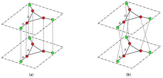
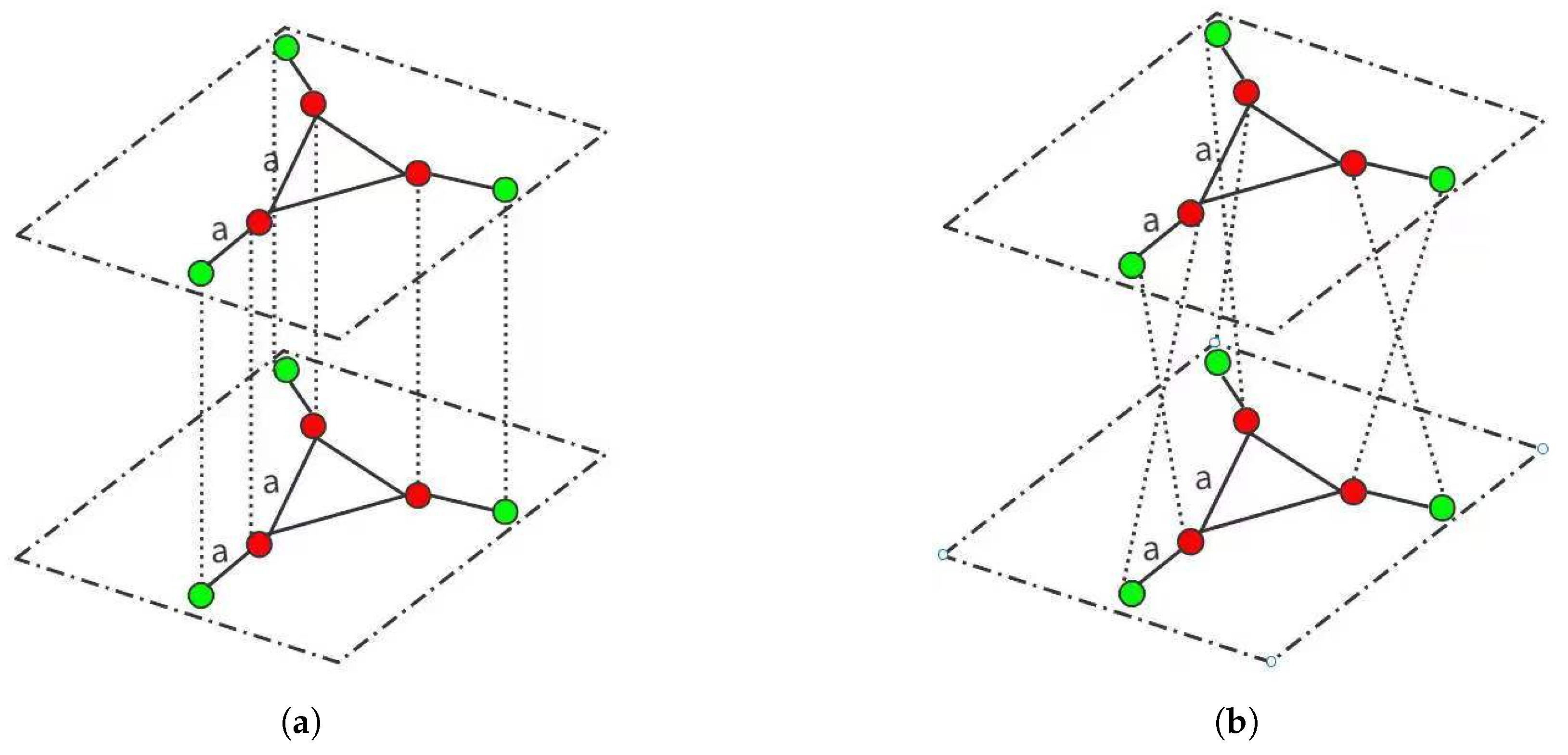
Double-layer positive and negative correlation networks are typical network structures with specific inter-layer connection patterns. When high-degree nodes connect to high-degree nodes, the structure is called the double-layer positive correlation network (see Figure 1a). The two layers of have the same topology, each consisting of n central nodes and n leaf nodes. The n central nodes form a complete network , i.e., the degree of each central node is n, and the degree of each leaf node is 1. Conversely, when high-degree nodes connect to low-degree nodes, it is called the double-layer negative correlation network (see Figure 1b). In , the central nodes of one layer are connected to the leaf nodes of the other layer, and the leaf nodes of one layer are connected to the central nodes of the other layer. The intra-layer coupling strength is a, and the inter-layer coupling strength is d.
Figure 1.
Double-layer network structures with different correlation patterns. Red nodes represent central nodes, green nodes represent leaf nodes, black solid lines represent intra-layer connections, and black dashed lines represent inter-layer connections. (a) Double-layer positive correlation network . (b) Double-layer negative correlation network .
The mathematical formulation of network dynamics under noise interference is given by
where L represents the Laplacian matrix of the network, and represents the Gaussian white noise interference.
3. Analytical Results and Coherence Analysis
3.1. Laplacian Spectrum and Coherence of Double-Layer Networks
3.1.1. Double-Layer Positive Correlation Network
The Laplacian matrix of the double-layer positive correlation network is given by
with
where is the identity matrix and is the all-ones matrix.
Remark 1
(Weighted L-spectrum for G+). The network can be viewed as the Cartesian product of the single-layer network (a corona product ) and a two-node graph H with edge weight d. According to Lemma 1, the eigenvalues of are , where . The single-layer network has the following eigenvalues:
- (multiplicity 1);
- (multiplicity 1);
- (multiplicity );
- (multiplicity ).
Therefore, the weighted L-spectrum of is
where
and .
Using the properties of roots of the quadratic equation, we have
The first-order coherence simplifies to
The second-order coherence simplifies to
3.1.2. Double-Layer Negative Correlation Network
The Laplacian matrix of is
with
Remark 2
(Weighted L-spectrum for G−). The eigenvalues of can be obtained by diagonalizing the block structure. Using the transformation matrix , we obtain
Thus, the eigenvalues of are the union of eigenvalues of and .
For ,
with eigenvalues
For ,
with eigenvalues
Thus, the weighted L-spectrum is
where
Using root–coefficient relationships, we obtain
Therefore, the first-order coherence is
The second-order coherence is
3.2. Three-Layer Network Analysis with Modified Laplacian Structure
3.2.1. Three-Layer Network Structures
To further investigate the coherence of the layered networks, we consider three-layer network structures including positive- and negative-correlation patterns. These networks consist of three identical layers, each containing n central nodes and n leaf nodes, with intra-layer coupling strength a and inter-layer coupling strength d. The two correlation patterns are defined as follows:
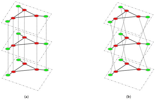
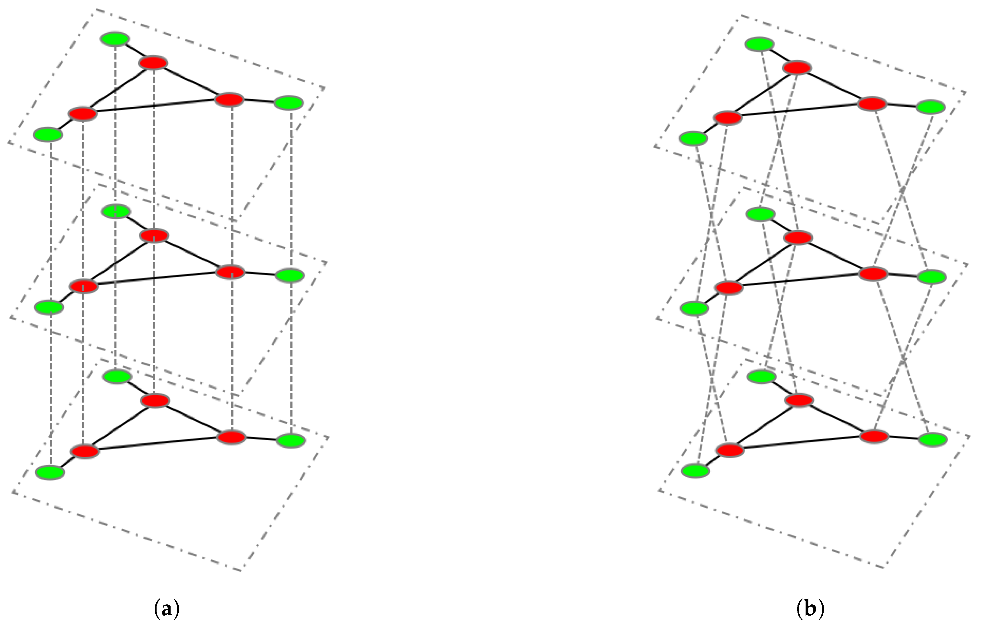
- Positive-correlation network (): Central nodes in each layer are connected to central nodes in other layers, and leaf nodes are connected to leaf nodes in other layers. Note that there is no direct connection between layer 1 and layer 3 (see Figure 2a).
- Negative-correlation network (): Central nodes in each layer are connected to leaf nodes in other layers, and leaf nodes are connected to central nodes in other layers. Note that there is no direct connection between layer 1 and layer 3 (see Figure 2b).
Figure 2.
Three-layer network structures with different correlation patterns. Red nodes represent central nodes, green nodes represent leaf nodes, black solid lines represent intra-layer connections, and black dashed lines represent inter-layer connections. In all configurations, there is no direct connection between layer 1 and layer 3. (a) Positively correlated three-layer network. (b) Negatively correlated three-layer network.
3.2.2. Three-Layer Positive Correlation Network
For the three-layer positive correlation network with modified structure, the Laplacian matrix is
where
Remark 3
(Weighted L-spectrum for G3+). The network is the Cartesian product , where is a three-node path graph with edge weight d. Applying Lemma 1, the Laplacian eigenvalues of are for and , with . This yields the following weighted L-spectrum:
where and .
Following Definition 1, the first-order and second-order coherence metrics simplify to
with
3.2.3. Three-Layer Negative Correlation Network
For the three-layer negative correlation network with modified structure, the Laplacian matrix is:
where ,
, and .
Remark 4
(Weighted L-spectrum for G3−). The weighted L-spectrum analysis of can be systematically derived by exploiting the network’s inherent symmetries and employing orthogonal block diagonalization techniques. The eigenvalue problem reduces to solving several matrix eigenvalue problems.
To exploit the symmetry , define the orthogonal matrix
Apply the similarity transformation . Because Q is orthogonal, has the same eigenvalues as . Direct computation yields a block-diagonal structure:
with each being a matrix:
Each involves the all-ones matrix . Construct an orthogonal matrix
where satisfies and . Then .
Apply the similarity transformation to each . This yields a further block diagonalization:
where is a matrix corresponding to the direction (where ), and is a matrix that repeats with multiplicity on the orthogonal complement (where ).
The matrices , , and are found to be
Their eigenvalues are
Thus, the six eigenvalues from the synchronization subspace (each of multiplicity 1) are
On the orthogonal complement where , the blocks become:
can be written as . The eigenvalues of are
Hence the eigenvalues of are and , each with multiplicity .
For and , they differ only by the sign of the off-diagonal d-term. Set
The four eigenvalues (each with multiplicity ) are
Collecting all contributions, the full Laplacian spectrum of is
The total number of nodes is , so the coherence prefactor is . Excluding the zero eigenvalue, the first- and second-order coherences are
The simplified expressions for the symmetric-mode contributions follow from the pairing of eigenvalues: and sum to T with product , while and sum to T with product .
4. Numerical Evaluations and Discussion
4.1. Double-Layer Network Coherence Analysis
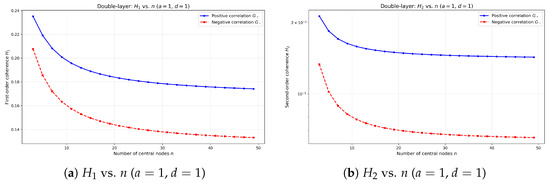
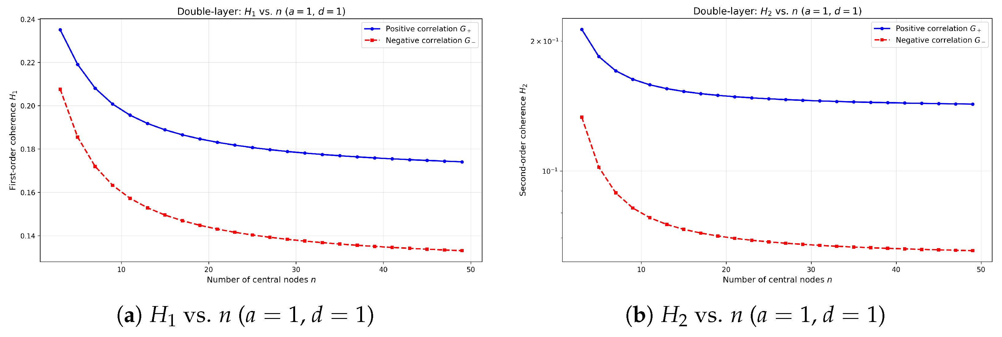
Figure 3 presents the first-order and second-order coherence for double-layer networks with fixed , . The left panel (a) shows versus n, demonstrating that negative-correlation networks () achieve consistently lower values than positive-correlation networks (). As n increases from 3 to 50, decreases from 0.235 to 0.174, and decreases from 0.208 to 0.133, indicating that both network types benefit from larger network size. However, the negative-correlation pattern consistently maintains a significant advantage, with approximately 24% lower than at .
Figure 3.
Double-layer network coherence analysis: (a) first-order coherence versus network size n; (b) second-order coherence versus network size n. Negative-correlation networks (, red dashed line) maintain better coherence as network size increases, while positive-correlation networks (, blue solid line) also improve but remain inferior.
The right panel (b) shows the second-order coherence as a function of n. The data reveal that is substantially lower than across all n, with the gap widening as n grows. For , while , confirming the superior noise-filtering capability of negatively correlated structures.
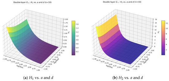
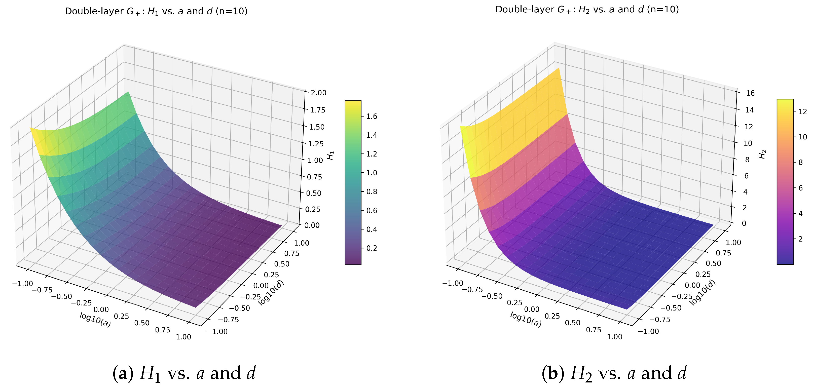
Figure 4 presents three-dimensional analyses of and as functions of both a and d for fixed . The surface plots confirm that negative-correlation networks achieve consistently lower coherence values across the entire parameter space. Both network types benefit from stronger intra-layer coupling (a) and inter-layer coupling (d), but negative correlation maintains its advantage throughout.
Figure 4.
Double-layer network : Three-dimensional surface plots (n = 10). Both and decrease with increasing a and d, showing improved coherence with stronger coupling.
4.2. Three-Layer Network Analysis
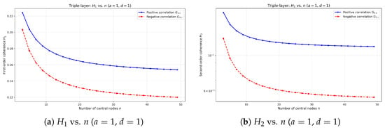
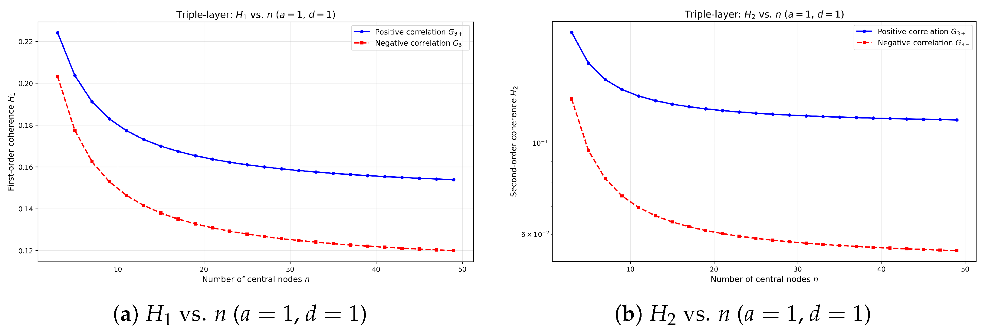
Figure 5 presents the first-order and second-order coherence for three-layer networks with fixed , . Similar to double-layer networks, negative-correlation patterns () achieve lower values than positive-correlation patterns (). As n increases, decreases from 0.224 to 0.154, while decreases from 0.203 to 0.120, demonstrating the superior coherence of negatively correlated three-layer networks. The right panel (b) shows significantly lower than , with the advantage becoming more pronounced as n increases (at , vs. ).
Figure 5.
Three-layer network coherence analysis: (a) first-order coherence versus network size n; (b) second-order coherence versus network size n. Negative-correlation networks () maintain superior coherence performance as network size increases.
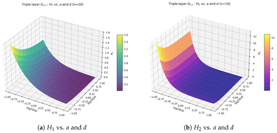
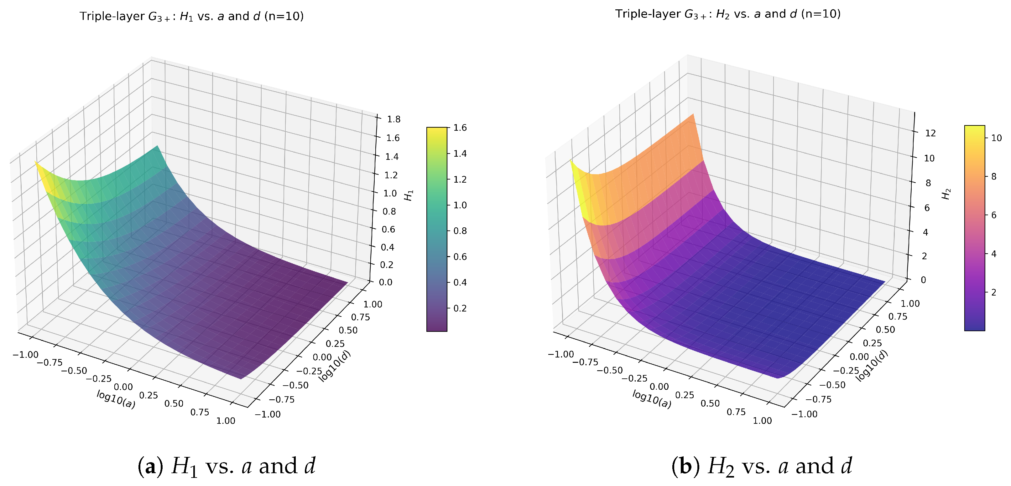
Figure 6 presents three-dimensional analyses of and as functions of both a and d for three-layer networks with fixed . The surface plots show similar trends to double-layer networks, with coherence decreasing as coupling strengths increase.
Figure 6.
Three-layer network : three-dimensional surface plots (n = 10). Both and show similar dependence on a and d as double-layer networks.
4.3. Comparative Analysis and Key Findings
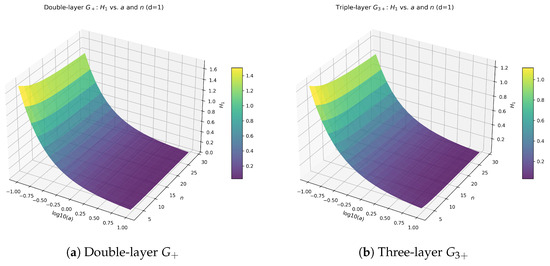
Figure 7 shows the dependence of on a and n for both double-layer and three-layer networks. The three-dimensional surface plots reveal that coherence decreases with increasing intra-layer coupling (a) and shows complex dependence on network size (n), with negative-correlation patterns consistently outperforming positive-correlation patterns.
Figure 7.
as functions of a and n (d = 1): (a) double-layer positive correlation network; (b) three-layer positive correlation network. Both show similar qualitative trends.
Table 1 summarizes key coherence values for selected network sizes. The data clearly show that negative-correlation networks achieve significantly lower coherence values, especially for larger n.
Table 1.
Key coherence values for selected network sizes (, ).
Statistical analysis of the improvement gained by negative-correlation patterns over the entire range to 50 reveals average improvements of for and for in double-layer networks, and for and for in three-layer networks. The improvement is more pronounced for second-order coherence, indicating that negative-correlation patterns are particularly effective at filtering high-frequency noise.
5. Conclusions
This paper studies the consensus problem in double-layer and three-layer positive- and negative-correlation networks. By constructing network Laplacian matrices and deriving their spectral distributions, explicit analytical expressions for network coherence are obtained. The robustness of coherence for positive- and negative-correlation networks under different parameters is systematically compared. Numerical evaluation results show that negative-correlation networks always have better coherence than positive-correlation networks; the coherence of both types of networks increases with the number of nodes and coupling strength, and the influence of node count is more significant. From the perspective of spectral analysis, the research reveals that connecting high-degree nodes to low-degree nodes across layers (negative correlation) can form a more balanced Laplacian eigenvalue distribution, thereby effectively improving consensus performance under noise. At the same time, the research results provide a theoretical basis for the design of robust layered networks in fields such as distributed sensing and multi-agent coordination. Future research will extend to more general correlated network structures, investigate the scaling law of coherence with the increase in layers, and explore the coherence evolution under dynamic inter-layer connection patterns.
Author Contributions
Conceptualization, D.H., J.Z. and Z.S.; methodology, Z.S., J.Z., D.H.; software, Z.S., Z.H.; validation, J.Z. and X.C.; formal analysis, Z.S., J.Z.; writing—original draft preparation, Z.S.; writing—review and editing, Z.S., D.H., J.Z., X.C. and Z.H.; supervision, X.C. and J.Z.; project administration, D.H.; funding acquisition, D.H. All authors have read and agreed to the published version of the manuscript.
Funding
This research was funded by the Natural Science Foundation of Xinjiang Uygur Autonomous Region (NSFXJ) (No. 2023D01A78, No. 202501A65), the National Natural Science Foundation of China (NSFC) (No. 12361110), Autonomous Region Level College Students’ Innovation and Entrepreneurship Training Program (No. S202410994017), and Xinjiang University Scientific Research (No. XJEDU2024P080), and The Foundation of Xinjiang Institute of Engineering (2024xgy092605).
Institutional Review Board Statement
Not applicable.
Informed Consent Statement
Not applicable.
Data Availability Statement
Data is contained within the article.
Conflicts of Interest
The authors declare no conflicts of interest.
References
- Consolini, L.; Morbidi, F.; Prattichizzo, D.; Tosques, M. Leader–follower formation control of nonholonomic mobile robots with input constraints. Automatica 2008, 44, 1343–1349. [Google Scholar] [CrossRef] [Scilit]
- Kim, B.; Ahn, H. Autonomous formation flight of multi-UAVs based on leader–follower approach. IEEE Syst. J. 2016, 10, 162–171. [Google Scholar] [CrossRef]
- Gao, H.; Li, W.; Cai, H. Distributed leader–follower formation control for multiple quadrotors with connectivity preservation. Drones 2022, 6, 266. [Google Scholar]
- Skardal, P.S.; Arola-Fernández, L.; Taylor, D.; Arenas, A. Higher-order interactions can better optimize network synchronization. Phys. Rev. Res. 2021, 3, 043193. [Google Scholar] [CrossRef] [Scilit]
- Chowdhary, S.; Kumar, A.; Cencetti, G.; Iacopini, I.; Battiston, F. Simplicial contagion in temporal higher-order networks. J. Phys. Complex. 2021, 2, 035019. [Google Scholar] [CrossRef] [Scilit]
- Li, Z.; Deng, Z.; Han, Z.; Alfaro-Bittner, K.; Barzel, B.; Boccaletti, S. Contagion in simplicial complexes. Chaos Solitons Fractals 2021, 152, 111307. [Google Scholar] [CrossRef] [Scilit]
- Fan, T.; Lü, L.; Shi, D.; Zhou, T. Characterizing cycle structure in complex networks. Commun. Phys. 2021, 4, 272. [Google Scholar] [CrossRef] [Scilit]
- Aktas, M.E.; Nguyen, T.; Jawaid, S.; Riza, R.; Akbas, E. Identifying critical higher-order interactions in complex networks. Sci. Rep. 2021, 11, 21288. [Google Scholar] [CrossRef] [Scilit]
- Zong, Y.; Dai, M.; Wang, X.; He, J.; Zou, J.; Su, W. Network coherence and eigentime identity on a family of weighted fractal networks. Chaos Solitons Fractals 2018, 109, 184–194. [Google Scholar] [CrossRef] [Scilit]
- Li, J.; Cai, M.; Tan, S.; Jia, T.; Lyu, X. Higher-order network modeling and information gain comparison based on citation big data. J. Syst. Sci. Math. Sci. 2021, 41, 2763–2775. [Google Scholar]
- Wang, X.; Xu, H.; Dai, M. First-order Network Coherence in 5-rose Graphs. Phys. A Stat. Mech. Its Appl. 2019, 527, 121129. [Google Scholar] [CrossRef] [Scilit]
- Wu, X.; Meng, H.; Lu, J.A. Synchronizability of double-layer chain networks with two inter-layer edges. Sci. China Inf. Sci. 2021, 64, 193101. [Google Scholar]
- Wei, X.; Wu, X.; Lu, J.A.; Wei, J.; Zhao, J.; Wang, Y. Synchronizability of two-layer correlation networks. Chaos 2021, 31, 103124. [Google Scholar] [CrossRef] [Scilit] [PubMed]
- Zhu, J.; Huang, D.; Jiang, H.; Bian, J.; Yu, Z. Synchronizability of multilayer variable coupling windmill-type networks. Mathematics 2021, 9, 2721. [Google Scholar] [CrossRef] [Scilit]
- Patterson, S.; Bamieh, B. Consensus and coherence in fractal networks. IEEE Trans. Control Netw. Syst. 2014, 1, 338–348. [Google Scholar] [CrossRef] [Scilit]
- Pirani, M.; Sundaram, S. Spectral properties of the grounded Laplacian matrix with applications to consensus in the presence of stubborn agents. IEEE Trans. Autom. Control 2016, 61, 509–515. [Google Scholar]
- Huang, D.; Bian, J.; Jiang, H.; Yu, Z. Consensus Indices of Two Layered Multi-Star Networks: An Application of Laplacian Spectrum. Front. Phys. 2021, 9, 803941. [Google Scholar] [CrossRef] [Scilit]
- Gao, H.; Zhu, J.; Chen, X.; Zhang, L.; Li, X. Coherence Analysis of Symmetric Star Topology Networks. Front. Phys. 2022, 10, 876994. [Google Scholar] [CrossRef] [Scilit]
- Sun, W.; Zhang, Q.; Li, Y. Network coherence and leader selection in complex multi-agent systems. IEEE Trans. Netw. Sci. Eng. 2023, 10, 789–801. [Google Scholar]
- He, W.; Xu, Z.; Du, W.; Chen, G.; Kubota, N.; Qian, F. Synchronization control in multiplex networks of nonlinear multi-agent systems. Chaos 2017, 27, 123104. [Google Scholar] [CrossRef] [Scilit]
- Liu, H.; Xu, J.; Li, Z.; Wang, X.; Lu, J.; Zeng, Z. Optimizing Synchronizability of Multilayer Networks Based on the Graph Comparison Method. IEEE Trans. Circuits Syst. I Regul. Pap. 2020, 67, 1740–1751. [Google Scholar] [CrossRef] [Scilit]
- Xu, M.; Lu, J.; Zhou, J. Synchronizability and eigenvalues of two-layer star networks. Acta Phys. Sin. 2016, 65, 028902. [Google Scholar] [CrossRef] [Scilit]
- Zhu, Y.; Liu, X.; Li, J. Synchronizability of multilayer variable coupling networks. Chaos 2021, 31, 063122. [Google Scholar]
- Sun, W.; Ding, Q.; Zhang, J.; Chen, F. Coherence in a family of tree networks with an application of Laplacian spectrum. Chaos 2014, 24, 043112. [Google Scholar] [CrossRef] [Scilit] [PubMed]
- Liu, J.; Zhang, X.; Cao, J. Structural properties of extended pseudo-fractal scale-free network with higher network efficiency. J. Complex Netw. 2024, 12, cnae023. [Google Scholar] [CrossRef] [Scilit]
- Zhang, L.; Zhong, J.; Lu, J. Finite-time synchronization of fractional-order complex networks via intermittent control. Neural Netw. 2021, 144, 11–20. [Google Scholar] [CrossRef] [Scilit] [PubMed]
- Sun, W.; Liu, S.; Li, Y. Coherence analysis of tree-symmetric networks under noise disturbance. IEEE Trans. Autom. Control 2022, 67, 4123–4130. [Google Scholar]
- Heinzelman, W.R.; Chandrakasan, A.; Balakrishnan, H. An application-specific protocol architecture for wireless microsensor networks. IEEE Trans. Wirel. Commun. 2002, 1, 660–670. [Google Scholar] [CrossRef] [Scilit]
- Li, X.; Wang, X. Negative correlation-based cross-layer power control for resilient WSNs against interference. IEEE Internet Things J. 2023, 10, 10890–10901. [Google Scholar]
- Fax, J.A.; Murray, R.M. Information flow and cooperative control of vehicle formations. IEEE Trans. Autom. Control 2004, 49, 1465–1476. [Google Scholar] [CrossRef] [Scilit]
- Huang, Y.; Meng, Z.; Dimarogonas, D.V. Prescribed performance formation control for second-order multi-agent systems with connectivity and collision constraints. Automatica 2024, 160, 111412. [Google Scholar] [CrossRef] [Scilit]
- Wang, Z.; Xia, C.; Chen, Z.; Chen, G. Epidemic Propagation with Positive and Negative Preventive Information in Multiplex Networks. IEEE Trans. Cybern. 2021, 51, 1454–1462. [Google Scholar] [CrossRef] [Scilit]
- Liu, Y.; Zhang, Q.; Sun, W. Laplacian spectrum of linear generalized phenylene-quadrilateral networks and its applications. Polycycl. Aromat. Compd. 2024, 44, 5609–5623. [Google Scholar] [CrossRef] [Scilit]
- Liu, Y.; Chen, J.; Sun, W. Exact determination of MFPT for random walks on rounded fractal networks with varying. J. Complex Netw. 2024, 12, cnae020. [Google Scholar] [CrossRef] [Scilit]
- Liu, J.; Guan, L.; Cao, J. Property analysis and coherence dynamics for tree-symmetric networks with noise disturbance. J. Complex Netw. 2024, 12, cnae029. [Google Scholar] [CrossRef] [Scilit]
- Zhang, Q.; Sun, W.; Xia, Y. Performance of leader–follower coherence for selecting leaders using node centrality indices. IEEE Trans. Circuits Syst. II 2024, 71, 4949–4953. [Google Scholar] [CrossRef] [Scilit]
- Sun, W.; Liu, S.; Li, Y. Coherence analysis of windmill networks with multiple leaders. Chaos Solitons Fractals 2023, 171, 113365. [Google Scholar]
- Liu, J.; Yu, M.; Cai, G.; Cao, J. The leader–follower coherence and spectral properties of weighted recursive networks under noise disturbance. Chaos Solitons Fractals 2026, 118060. [Google Scholar] [CrossRef] [Scilit]
- Patterson, S.; Yi, Y.; Zhang, Z. A resistance-distance-based approach for optimal leader selection in noisy consensus networks. IEEE Trans. Control Netw. Syst. 2019, 6, 191–201. [Google Scholar] [CrossRef] [Scilit]
- Patterson, S.; McGlohon, N.; Dyagliev, K. Optimal k-leader selection for coherence and convergence rate. IEEE Trans. Control Netw. Syst. 2017, 4, 523–532. [Google Scholar] [CrossRef] [Scilit]
- Fitch, K.; Leonard, N. Information centrality and optimal leader selection in noisy networks. In Proceedings of the 52nd IEEE Conference on Decision and Control, Florence, Italy, 10–13 December 2013; pp. 7510–7515. [Google Scholar]
- Chen, J.; Sun, W.; Wang, J. Topology design for leader-follower coherence in noisy asymmetric networks. Phys. Scr. 2023, 98, 015215. [Google Scholar] [CrossRef] [Scilit]
- Liu, J.; Zhang, X.; Cao, J.; Chen, L. Mean First-Passage Time and Robustness of Complex Cellular Mobile Communication Network. IEEE Trans. Netw. Sci. Eng. 2024, 11, 3066–3076. [Google Scholar] [CrossRef] [Scilit]
- Zhang, Q.; Sun, W.; Li, Y. Robustness of network coherence in hierarchical structures under edge failures. Phys. Rev. E 2023, 107, 024301. [Google Scholar]
- Cvetkovic, D.; Rowlinson, P.; Simic, S. An Introduction to the Theory of Graph Spectra; Cambridge University Press: Cambridge, UK, 2010. [Google Scholar]

Disclaimer/Publisher’s Note: The statements, opinions and data contained in all publications are solely those of the individual author(s) and contributor(s) and not of MDPI and/or the editor(s). MDPI and/or the editor(s) disclaim responsibility for any injury to people or property resulting from any ideas, methods, instructions or products referred to in the content. |
© 2026 by the authors. Licensee MDPI, Basel, Switzerland. This article is an open access article distributed under the terms and conditions of the Creative Commons Attribution (CC BY) license.