Functional Data Analysis of Particulate Matter (PM₁₀) in Chungbuk, Korea: An Application of Penalized B-Spline Smoothing and Functional Inference

Abstract

Functional data analysis (FDA) provides a framework for representing high-frequency or longitudinal observations as smooth functions, enabling principled dimension reduction and feature extraction. We develop a B-spline-based FDA approach with a total variation penalty to model daily PM₁₀ trajectories, with smoothing parameters selected via AIC and BIC. Functional principal component analysis (FPCA) is applied to identify dominant temporal patterns, including overall levels, seasonal deviations, and episodic peaks, while preserving abrupt changes. This methodology allows for flexible and interpretable summaries of complex time series and comparisons across spatial or temporal domains. We apply this framework to 365-day PM₁₀ curves from 28 monitoring stations in Chungcheongbuk-do, Korea, for 2022. The first four principal components capture over 80% of total variation, reflecting winter peaks, early spring fluctuations, and summer troughs. Urban–rural contrasts examined via functional two-sample t-tests and FPCA scores reveal minimal differences at the functional level. This study illustrates how FDA, combined with penalized B-splines, can concisely summarize complex temporal dynamics, quantify dominant patterns, and offer a flexible framework for analyzing environmental time series and other functional datasets. The approach provides a general strategy for understanding temporally structured processes in various scientific fields.

1. Introduction

Functional data analysis (FDA) is a branch of statistics that treats each observational unit as a function, curve, or trajectory evolving over a continuum such as time, space, or wavelength, rather than as a finite-dimensional vector [1,2]. In FDA, the basic data object is a smooth function, observed on a dense or possibly irregular grid, and the primary inferential targets include the mean function, covariance structure, and low-dimensional representations such as functional principal components scores. This perspective has proved particularly powerful in scientific fields where modern sensing technologies routinely generate high-frequency, longitudinal, or image-type measurements; examples include growth curves, spectrometric data, biomechanical trajectories, and environmental time series [1,3]. By explicitly exploiting the smoothness and functional structure of the data, FDA provides a principled framework for regularization, noise reduction, and dimension reduction that is difficult to achieve with purely multivariate methods.

From a methodological standpoint, FDA combines ideas from nonparametric regression, smoothing splines, and functional approximation theory. In particular, basis expansions—such as B-splines, Fourier series, and wavelets—play a central role in representing functional observations as linear combinations of basis functions with a relatively small number of coefficients [1,2]. This representation facilitates the use of penalized likelihood or penalized least squares criteria, where roughness penalties enforce smoothness and prevent overfitting. Among various basis systems, B-splines are widely used in practice due to their excellent numerical properties, local support, and flexibility in handling complex designs and boundary behavior. Recent research has further developed penalized B-spline estimators that incorporate total variation (TV) penalties on derivatives, providing an attractive compromise between smooth approximation and the ability to capture sharp changes or structural breaks in functional relationships [4].

In parallel with these methodological advances, there has been growing interest in applying FDA to environmental and public-health problems, where the underlying processes are naturally viewed as time-varying curves or surfaces [3]. Ambient air pollution, and in particular particulate matter (PM), is a representative example. Particulate matter with aerodynamic diameter less than or equal to $10 \mathsf{\mu }\mathrm{m}$ (PM₁₀) or $2.5 \mathsf{\mu }\mathrm{m}$ (PM_2.5) has been identified as a major risk factor for a broad range of adverse health outcomes, including respiratory disease, cardiovascular disease, and cancer [5]. The International Agency for Research on Cancer (IARC) classified outdoor air pollution and particulate matter as carcinogenic to humans and emphasized that outdoor air pollution is a leading environmental cause of cancer deaths worldwide [6]. These findings have reinforced the need for accurate statistical methods to characterize temporal patterns in particulate concentrations and to assess their health and policy implications.

Reflecting the accumulating epidemiological and toxicological evidence, the World Health Organization (WHO) issued updated Global Air Quality Guidelines in 2021, substantially tightening recommended exposure limits for PM_2.5 and NO₂ relative to the 2005 guidelines [7,8]. The new guidelines recommend, for example, that the annual mean concentration of PM_2.5 should not exceed $5 \mathsf{\mu }\mathrm{g}/{\mathrm{m}}^3$, a target that is currently violated in many urban areas around the world [8]. The WHO and collaborating societies have emphasized that even relatively low concentrations of particulate matter are associated with increased mortality and morbidity, and that there appears to be no safe threshold below which adverse health effects can be ruled out [8]. In this context, statistical models that can capture the full temporal evolution of pollutant concentrations—including seasonal patterns, short-term peaks, and long-term trends—are essential to inform risk assessment and environmental regulation.

In Korea, public concern over particulate matter has increased markedly since the early 2010s, driven in part by frequent high-concentration episodes and extensive media coverage. Empirical analyses of national monitoring data have documented long-term trends and regional disparities in PM₁₀ concentrations, as well as changes in the frequency and persistence of high-pollution events [9]. For instance, Yeo and Kim [9] showed that, while annual mean PM₁₀ levels have generally decreased since the early 2000s, the occurrence of high-concentration cases remains non-negligible and exhibits distinct spatial patterns across provinces. At a more local scale, several studies have examined the current state of fine dust and its emission sources in specific regions, including Chungcheongbuk-do, highlighting the combined influence of industrial activities, traffic, and transboundary transport on regional air quality [10,11]. These findings underscore the importance of region-specific analyses that reflect local emission structures, meteorological conditions, and topographical features.

Chungcheongbuk-do (Chungbuk) is a landlocked province in the central region of South Korea, characterized by a mix of urban, industrial, and rural areas. Owing to its geographical location and industrial structure, Chungbuk experiences complex interactions between locally emitted pollutants and those transported from other regions or across national borders [10,11]. Previous work on Chungbuk has mainly focused on descriptive analyses of long-term averages, emission inventories, and source apportionment [10]. However, less attention has been paid to the detailed temporal dynamics of PM₁₀ concentrations at daily or hourly scales, such as seasonal variation, intra-annual heterogeneity, and short-term peak behaviors. Given the increasing policy interest in region-specific mitigation strategies—for example, targeted emission controls and early-warning systems—there is a clear need for statistical methodologies that can summarize, compare, and model these complex temporal patterns in a systematic manner.

From a statistical perspective, time series of pollutant concentrations can naturally be viewed as functional data when measurements are collected on a fine and regular grid, such as daily or hourly monitoring records over multiple years. In this setting, each year (or season) can be regarded as a smooth curve representing the trajectory of PM₁₀ concentrations, and FDA tools can be deployed to explore the main modes of temporal variation and to perform inference on their determinants [1,2]. Functional principal component analysis (FPCA), in particular, provides a flexible and interpretable way to decompose temporal variability into orthogonal components that capture, for example, overall level, seasonal amplitude, and timing of high-pollution episodes. This approach has been successfully applied in various environmental and epidemiological contexts, including analyses of mortality time series and air quality indicators [3,12]. By combining FPCA with penalized B-spline representations and appropriate roughness penalties, one can obtain smooth yet data-adaptive estimates of these components, even in the presence of irregular sampling or measurement noise [2,4].

The increasing visibility of FDA in both theory and applications is also reflected in recent developments in the literature, including functional time series analysis, functional regression, and functional principal component analysis under complex dependence structures [12]. These works demonstrate that FDA methods can be effectively integrated with modern dependence modeling, such as copula-based dynamic conditional correlation models, to analyze high-dimensional and temporally dependent functional data. Against this backdrop, the present study aims to contribute to the growing FDA literature by developing and applying a B-spline based functional principal component framework tailored to the analysis of PM₁₀ concentration curves in Chungcheongbuk-do. Specifically, we focus on (i) constructing smooth functional representations of daily PM₁₀ trajectories using penalized B-splines, (ii) extracting dominant modes of temporal variation via FPCA, and (iii) interpreting the resulting components in terms of seasonal patterns, high-concentration episodes, and long-term trends. The proposed approach not only yields a parsimonious description of complex temporal dynamics but also provides a basis for subsequent modeling and policy-relevant interpretation in the context of air quality management. Although the methods themselves are well-established, the primary contribution of this study lies in applying them to PM₁₀ data in a novel manner, providing new insights into seasonal patterns, high-concentration episodes, and long-term trends.

2. Related Work

Research on particulate matter (PM) and its health and environmental effects has expanded rapidly over the past two decades. Epidemiological evidence now demonstrates consistent associations between exposure to fine and coarse particles and a wide range of adverse outcomes, including respiratory and cardiovascular morbidity and mortality [5,8]. Based on these accumulating results, several international agencies have strengthened regulatory guidelines and emphasized the absence of a clearly defined threshold below which health effects do not occur [6,7]. These developments have motivated the need for statistical methods capable of capturing complex temporal patterns in pollution data and linking them to potential health and policy implications.

2.1. Statistical Approaches to Air Pollution Time Series

Traditional analyses of air quality time series have relied largely on regression-based and autoregressive models, focusing on estimating long-term trends, seasonal components, and short-term fluctuations. Generalized additive models (GAMs), for example, have been widely adopted to study nonlinear relationships between pollutants and meteorological predictors, as well as to estimate exposure–response functions [13]. More recently, hierarchical Bayesian models, state–space models, and machine learning approaches have been used to model spatial and temporal dependence and to improve predictive performance [11,14]. Although powerful, many of these models treat pollutant concentrations as multivariate vectors rather than continuous curves, potentially overlooking the functional nature of the underlying processes. For example, GAMs or autoregressive models may effectively capture short-term dependence or pointwise exposure–response relationships, but they can fail to reveal multi-day episodic pollution events or station-specific seasonal shifts, which are important features of PM₁₀ time series.

2.2. Functional Data Analysis in Environmental Applications

Functional data analysis (FDA) provides a natural alternative framework in settings where densely observed time series can be regarded as smooth curves [1,2]. In FDA, each temporal trajectory—for example, the daily concentration of PM over one year—is modeled as a function defined on a continuous domain. This representation enables direct study of functional features, such as the evolution of peaks, the timing of seasonal shifts, and the correlation structure across time.

FDA techniques have been successfully applied across environmental science. Typical applications include temperature and precipitation curves, hydrological flow records, oceanographic profiles, and mortality and morbidity time series influenced by environmental exposures [3]. Functional regression models allow pollutant curves to serve either as predictors or responses, thereby linking exposure trajectories to clinical or policy outcomes in a flexible manner [15]. In addition, functional hypothesis testing has been developed to compare mean curves between groups or time periods, often relying on permutation-based procedures and maximum-type statistics to account for functional dependence [2].

2.3. Basis Expansion and Penalization

Central to FDA is the representation of functional observations using basis expansions, such as Fourier bases, wavelets, and B-splines. Among these, B-spline bases have proven especially attractive due to their local support, numerical stability, and adaptability to irregular designs [16]. Penalization strategies—including roughness penalties and total variation (TV) penalties—regularize the fitted functions by discouraging excessive wiggliness while still preserving meaningful structure.

In particular, penalized B-spline estimators incorporating TV penalties on higher-order derivatives offer an appealing compromise between smoothness and flexibility. They allow for the detection of relatively abrupt changes while retaining stable estimation elsewhere, a feature particularly relevant for pollution data characterized by episodic peaks [4]. Such approaches have been successfully applied in regression and smoothing contexts and continue to receive attention in both theory and applications.

2.4. Functional Principal Component Analysis (FPCA)

Functional principal component analysis (FPCA) is one of the most widely used tools in FDA. FPCA decomposes the covariance operator of functional data into orthogonal modes, each describing a distinct source of temporal variation [1]. The first few principal components usually explain the majority of the total variability and often correspond to interpretable temporal features, such as overall pollution level, seasonal amplitude, or shifts in the timing of peaks.

Recent contributions have extended FPCA to deal with dependence, nonstationary structures, and high-dimensional functional datasets. For example, recently published several studies have explored FPCA in combination with dynamic correlation structures and copula-based dependence models, illustrating its versatility in complex time series settings [12,17]. These methodological developments provide a foundation for applying FPCA to air quality data, where temporal dependence and heterogeneous variability are intrinsic characteristics.

2.5. Motivation for the Present Study

Despite the rapid methodological progress and the proliferation of pollution studies, region-specific analyses using FDA remain relatively limited in Korea, particularly at the provincial level. Previous work on Chungcheongbuk-do has mainly focused on descriptive statistics, emission inventories, and source apportionment analyses [9,10], with less attention paid to the functional structure of daily particulate matter trajectories.

The present study seeks to bridge this gap by developing and applying an FDA-based framework tailored to PM₁₀ concentrations in Chungbuk. By integrating penalized B-spline smoothing with FPCA and functional hypothesis testing, we aim to provide a detailed, interpretable, and statistically rigorous description of seasonal patterns, episodic peaks, and temporal variability in regional air quality. This line of research contributes not only to the growing literature on FDA in environmental science but also to policy-relevant understanding of particulate pollution dynamics in Korea.

3. Methodology

We briefly describe the methodological framework used in this study. The analysis consists of four main steps: (i) representation of daily PM₁₀ curves as functional observations; (ii) penalized B-spline smoothing with total variation (TV) penalty; (iii) functional two-sample testing; and (iv) functional principal component analysis (FPCA). Throughout, the focus is on tools that are flexible, computationally stable, and well-suited to environmental time-series data.

3.1. Functional Representation

Let $Y_i\left(t_j\right)$ denote the observed PM₁₀ concentration at station i ($i=1,\dots ,n$) on day $t_j$ ($j=1,\dots ,T$). We assume that these discrete measurements arise from an underlying smooth function $X_i\left(t\right)$ observed with measurement error:

$$Y_i\left(t_j\right)=X_i\left(t_j\right)+{\epsilon }_{ij},{\epsilon }_{ij}\sim \mathrm{i}.\mathrm{i}.\mathrm{d}.(0,{\sigma }^2),$$

(1)

where $X_i\left(t\right)$ is defined on the continuous domain $t\in [0,1]$ (after linear rescaling of the calendar year). Note that time is rescaled to [0, 1] for convenience, with $t=0$ and $t=1$ representing 1 January and 31 December, so seasonal interpretation is preserved.

The goal of smoothing is to obtain stable estimates ${\widehat{X}}_i\left(t\right)$ that retain the important temporal features of the original trajectories.

3.2. B-Spline Basis Expansion

Each smooth curve $X_i\left(t\right)$ is represented using a finite number of cubic B-spline basis functions:

$$X_i\left(t\right)\approx \sum _{k=1}^K{\beta }_{ik}{B}_k\left(t\right)=\mathbf{B}{\left(t\right)}^{\top }{\mathit{\beta }}_i,$$

(2)

where $\mathbf{B}\left(t\right)={\{B_1\left(t\right),\dots ,B_K\left(t\right)\}}^{\top }$ denotes the spline basis and ${\mathit{\beta }}_i={({\beta }_{i1},\dots ,{\beta }_{iK})}^{\top }$ are the station-specific coefficients. Cubic B-splines ensure continuity of the first and second derivatives and offer local support and numerical stability [16].

3.3. Penalized Spline Smoothing with TV Penalty

Following [4], we estimate ${\mathit{\beta }}_i$ by solving the penalized least squares problem:

$$\underset{{\mathit{\beta }}_i}{min}\left\{\sum _{j=1}^T{\left(Y_i\left(t_j\right)-\mathbf{B}{\left(t_j\right)}^{\top }{\mathit{\beta }}_i\right)}^2+\lambda \mathrm{TV}\left({\displaystyle \frac{d^3}{d{t}^3}}{X}_i\left(t\right)\right)\right\},$$

(3)

where $\lambda \ge 0$ controls the degree of smoothness and $\mathrm{TV}(·)$ denotes the total variation functional.

For a function f defined on $[0,1]$, total variation is

$$\mathrm{TV}\left(f\right)=\underset{\mathcal{P}}{sup}\sum _{m=0}^{\left|\mathcal{P}\right|-1}\left|f\left(x_{m+1}\right)-f\left(x_m\right)\right|,$$

(4)

where the supremum is taken over all finite partitions $\mathcal{P}=\{0=x_0<\cdots <x_{\left|\mathcal{P}\right|}=1\}$.

In the cubic B-spline setting, penalizing the total variation in the third derivative is closely related to automatic knot selection and yields smooth yet adaptive estimates [4].

We select $\lambda$ by minimizing information criteria:

$$\mathrm{AIC}\left(\lambda \right)=T\log \left({\widehat{\sigma }}^2\left(\lambda \right)\right)+2\mathrm{edf}\left(\lambda \right),\mathrm{BIC}\left(\lambda \right)=T\log \left({\widehat{\sigma }}^2\left(\lambda \right)\right)+\log \left(T\right)\mathrm{edf}\left(\lambda \right),$$

(5)

where $\mathrm{edf}\left(\lambda \right)$ denotes the effective degrees of freedom. In practice, Akaike information criterion (AIC; [18]) tends to favor less oversmoothing than the Bayesian information criterion (BIC; [19]), which is beneficial for pollution data exhibiting episodic peaks. In the present setting with densely observed daily series, information-criterion-based selection provides a computationally efficient and stable choice, and allows direct comparison between AIC and BIC in terms of smoothness and peak preservation. Note that alternative criteria, such as cross-validation, could also be used to select the smoothing parameter.

3.4. Exploratory Functional Quantities

Given smoothed curves $\left\{{\widehat{X}}_i\left(t\right)\right\}$, the mean and variance functions are

$$\overline{X}\left(t\right)={\displaystyle \frac{1}{n}}\sum _{i=1}^n{\widehat{X}}_i\left(t\right),\mathrm{Var}\left(t\right)={\displaystyle \frac{1}{n-1}}\sum _{i=1}^n{\left({\widehat{X}}_i\left(t\right)-\overline{X}\left(t\right)\right)}^2.$$

(6)

The covariance surface is estimated as

$$\mathrm{Cov}(s,t)={\displaystyle \frac{1}{n-1}}\sum _{i=1}^n\left({\widehat{X}}_i\left(s\right)-\overline{X}\left(s\right)\right)\left({\widehat{X}}_i\left(t\right)-\overline{X}\left(t\right)\right).$$

(7)

3.5. Functional Two-Sample t-Test

Suppose the stations are divided into two groups, Group 1 (urban) and Group 2 (rural), with sample sizes $n_1$ and $n_2$. The pointwise test statistic proposed in [2] is

$$T\left(t\right)={\displaystyle \frac{\left|{\overline{X}}_1\left(t\right)-{\overline{X}}_2\left(t\right)\right|}{\sqrt{{\mathrm{Var}}_1\left(t\right)/n_1+{\mathrm{Var}}_2\left(t\right)/n_2}}},$$

(8)

where ${\overline{X}}_g\left(t\right)$ and ${\mathrm{Var}}_g\left(t\right)$ denote the group-specific mean and variance functions.

To obtain global inference, we compute the maximum-type statistic ${max}_{t}T\left(t\right)$ and evaluate its null distribution using permutation-based resampling, thus preserving the functional dependence.

3.6. Functional Principal Component Analysis (FPCA)

FPCA decomposes temporal variability through the eigen-decomposition of the covariance operator. The eigenfunctions $\left\{{\xi }_k\left(t\right)\right\}$ solve

$${\int }_0^1\mathrm{Cov}(s,t){\xi }_k\left(t\right)dt={\rho }_k{\xi }_k\left(s\right),$$

(9)

where ${\rho }_k$ are the eigenvalues ordered ${\rho }_1\ge {\rho }_2\ge \cdots \ge 0$.

Each curve admits the Karhunen–Loève representation:

$$X_i\left(t\right)=\mu \left(t\right)+\sum _{k=1}^{\infty }{\alpha }_{ik}{\xi }_k\left(t\right),{\alpha }_{ik}={\int }_0^1\left(X_i\left(t\right)-\mu \left(t\right)\right){\xi }_k\left(t\right)dt,$$

(10)

where ${\alpha }_{ik}$ are uncorrelated principal component scores with $\mathrm{Var}\left({\alpha }_{ik}\right)={\rho }_k$. Note that Table 1 provides a brief summary of the key symbols used in the FPCA framework.

Table 1. Summary of key notation used in the FPCA framework.

Notation	Description
$X_i\left(t\right)$	Smoothed PM10 concentration curve for station i
$\mu \left(t\right)$	Mean function across all stations
${\xi }_k\left(t\right)$	k-th functional principal component (eigenfunction)
${\alpha }_{ik}$	FPCA score of station i for component k
${\rho }_k$	Eigenvalue corresponding to the k-th component

In practice, only the first few components explaining the majority of total variance are retained, yielding a parsimonious but interpretable description of temporal behavior in PM₁₀ concentrations [1,12].

Overall, the methodological framework presented in this section adopts an FDA perspective to treat PM₁₀ concentrations as smooth temporal processes rather than discrete observations. In contrast to conventional time-series approaches, which typically focus on short-term dependence structures or pointwise temporal dynamics, the FDA framework represents each station’s record as a continuous trajectory defined over a common domain.

In contrast, the total variation penalty adopted in this study is naturally aligned with the methodological objective of capturing both structural commonality and localized heterogeneity across multiple functional trajectories. By allowing for roughness to be concentrated at a limited number of time points, the total variation penalty yields piecewise-smooth representations in which shared temporal patterns are preserved while station-specific abrupt changes are retained when supported by the data. This feature is particularly relevant for PM₁₀ concentrations, where abrupt concentration increases associated with episodic environmental events may differ across regions and should not be uniformly penalized as roughness. Consequently, the total variation penalty provides a more appropriate roughness penalty than derivative-based alternatives for modeling collections of functional curves with both common and region-specific temporal features.

Compared with GAM-based analyses that emphasize regression relationships and conditional mean effects at individual time points, the proposed approach facilitates direct comparison of entire temporal profiles across monitoring stations. By combining penalized B-spline smoothing with FPCA, the framework provides a parsimonious representation of dominant modes of temporal variability and establishes a coherent basis for functional inference on seasonal patterns and regional differences in air pollution dynamics.

4. Data Analysis: PM₁₀ Concentrations in Chungbuk

In this section, we apply the proposed functional data analysis framework to daily PM₁₀ concentrations monitored across Chungcheongbuk-do (Chungbuk), Korea. The primary objective is to describe temporal variation, evaluate potential differences between urban and rural environments, and identify dominant modes of variability through functional principal component analysis (FPCA).

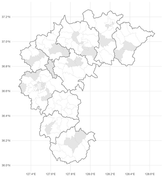
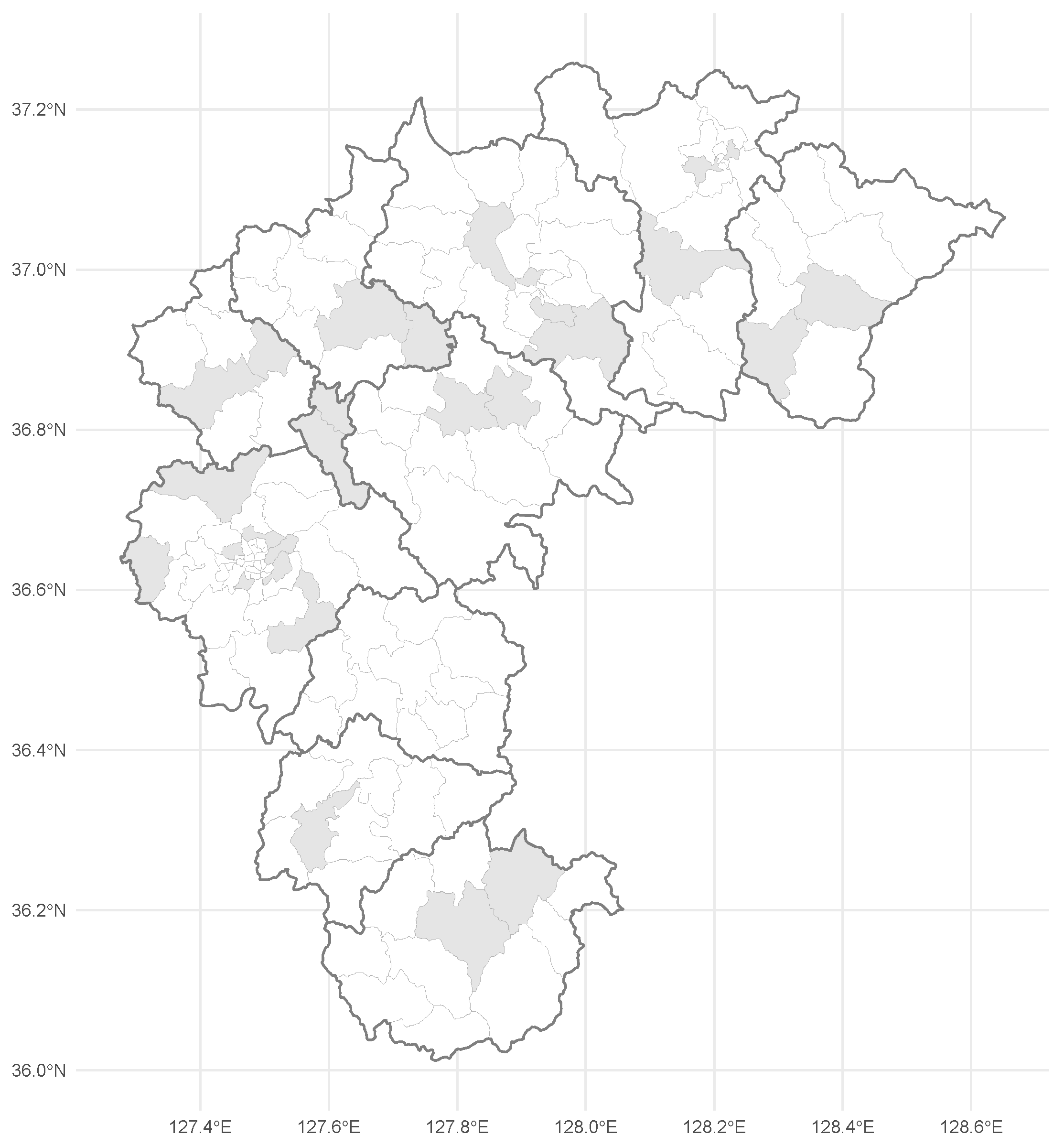
Air-quality measurements were obtained from AirKorea, the national monitoring network that records several major atmospheric pollutants, including SO₂, NO₂, O₃, CO, PM₁₀, and PM_2.5. The PM₁₀ values are determined using either gravimetric methods or the $\beta$-ray absorption method, and results are reported in $\mathsf{\mu }\mathrm{g}/{\mathrm{m}}^3$. During 2022, a total of 30 monitoring stations operated within the province. To ensure reliability of inference, stations exhibiting more than 15% missing daily values (equivalent to at least 55 missing days) were removed. After this screening step, 28 stations remained and Figure 1 illustrates the administrative regions in which these stations are located. In Figure 1, thick boundary lines indicate city and county boundaries, while thin lines represent lower-level administrative units (eup, myeon, and dong). Gray-shaded regions indicate administrative areas where monitoring stations are located. Meanwhile, the total number of missing days across all stations was only 36. Because the proportion of missingness was small, these values were omitted rather than imputed.

Figure 1. Administrative regions of the 28 PM monitoring stations. Thick boundary lines indicate city and county boundaries, and thin lines represent lower-level administrative units (eup, myeon, and dong). Gray shading highlights regions with monitoring stations.

Korea typically experiences pronounced seasonal fluctuations in particulate concentrations. For this reason, the complete calendar year from January to December 2022 was analyzed, allowing us to capture recurring features such as winter peaks, spring transition periods, summer troughs, and late-autumn increases. Note that 2022 was primarily selected because it was the year in which data collection and analysis were initiated. Historical records from 2018 to 2022 indicate that annual mean PM₁₀ concentrations and key meteorological variables (temperature, wind speed, and precipitation) were generally consistent with previous years, as shown in Supplemental Figure S1, suggesting that 2022 was not anomalous and is suitable for examining typical seasonal patterns.

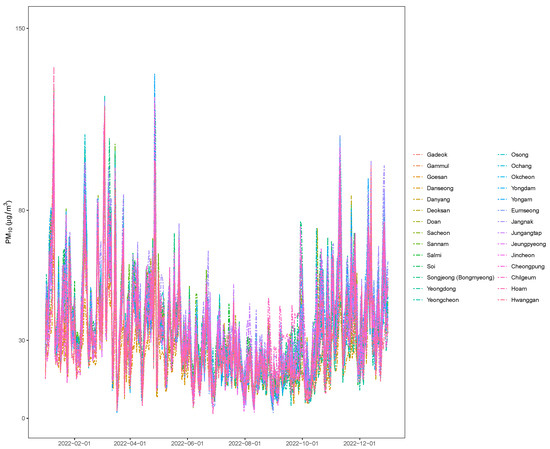
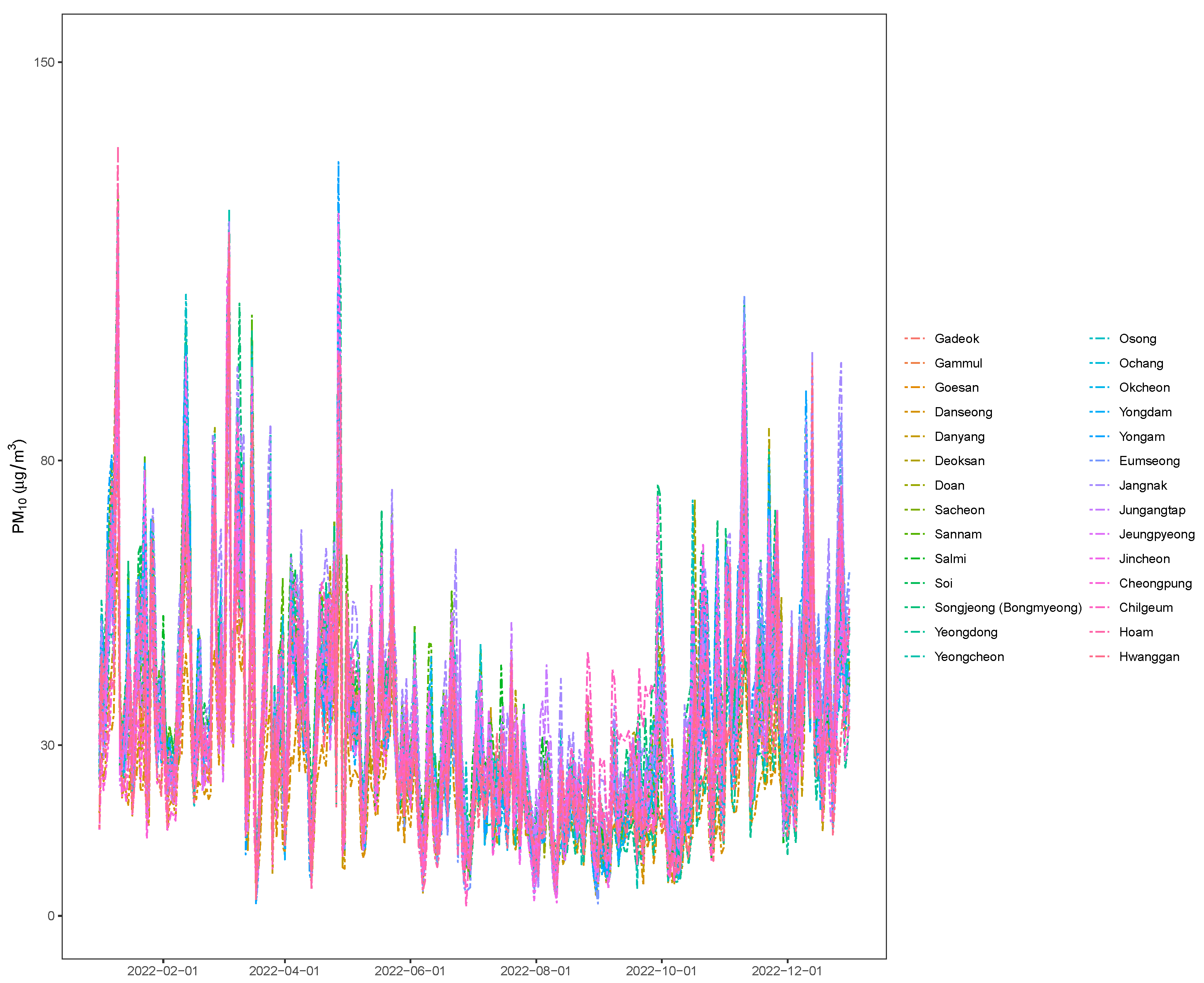
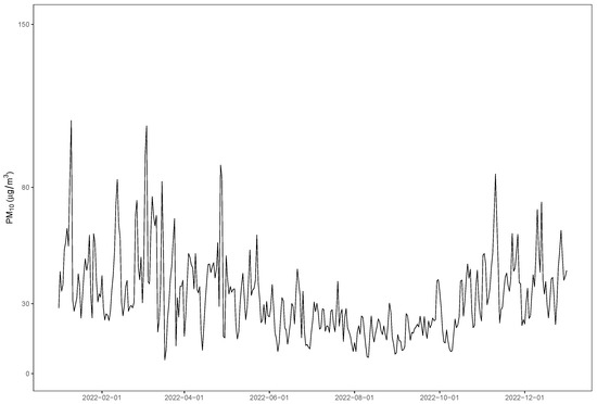
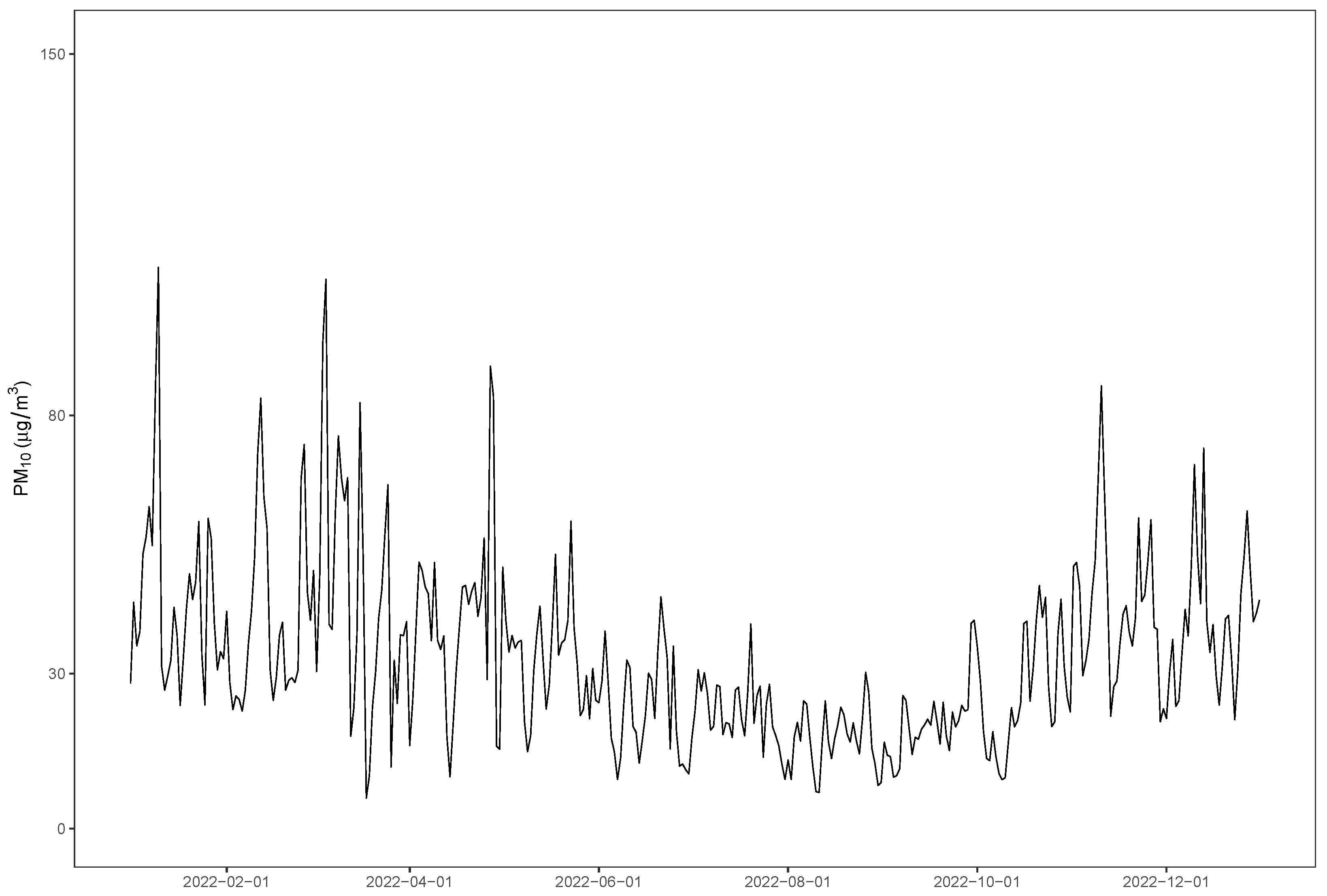
Figure 2 displays the daily PM₁₀ trajectories for all 28 stations. Most stations share a broadly similar temporal pattern: concentrations rise during winter and early spring, decline substantially during summer, and increase again toward the end of the year. Figure 3 summarizes these dynamics by showing the overall mean curve, in which several pronounced short-term surges are visible, particularly in January–March, May, and November.

Figure 2. Daily PM₁₀ concentrations for 28 monitoring stations in Chungbuk over 2022. Each curve represents one station.

Figure 3. Overall mean daily PM₁₀ concentration across the 28 stations.

To investigate spatial heterogeneity related to population density, monitoring sites were classified into urban (population ≥ 50,000) and rural (population < 50,000) groups. The urban group consists of stations located in Cheongju, Chungju, and Jecheon, whereas the remaining sites, such as those in Danyang, Goesan, Yeongdong, Eumseong, Jeungpyeong, Jincheon, and Okcheon, are categorized as rural. Supplemental Figure S2 presents daily curves for the urban stations with the overall mean superimposed. Several locations, including Songjeong in Cheongju and Jangrak in Jecheon, frequently record concentrations above the provincial average. By contrast, many rural stations remain slightly below the mean throughout most of the year; for instance, Danseong in Danyang consistently exhibits the lowest levels, as shown together with other rural stations in Supplemental Figure S3.

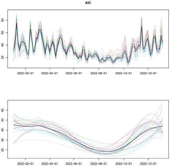
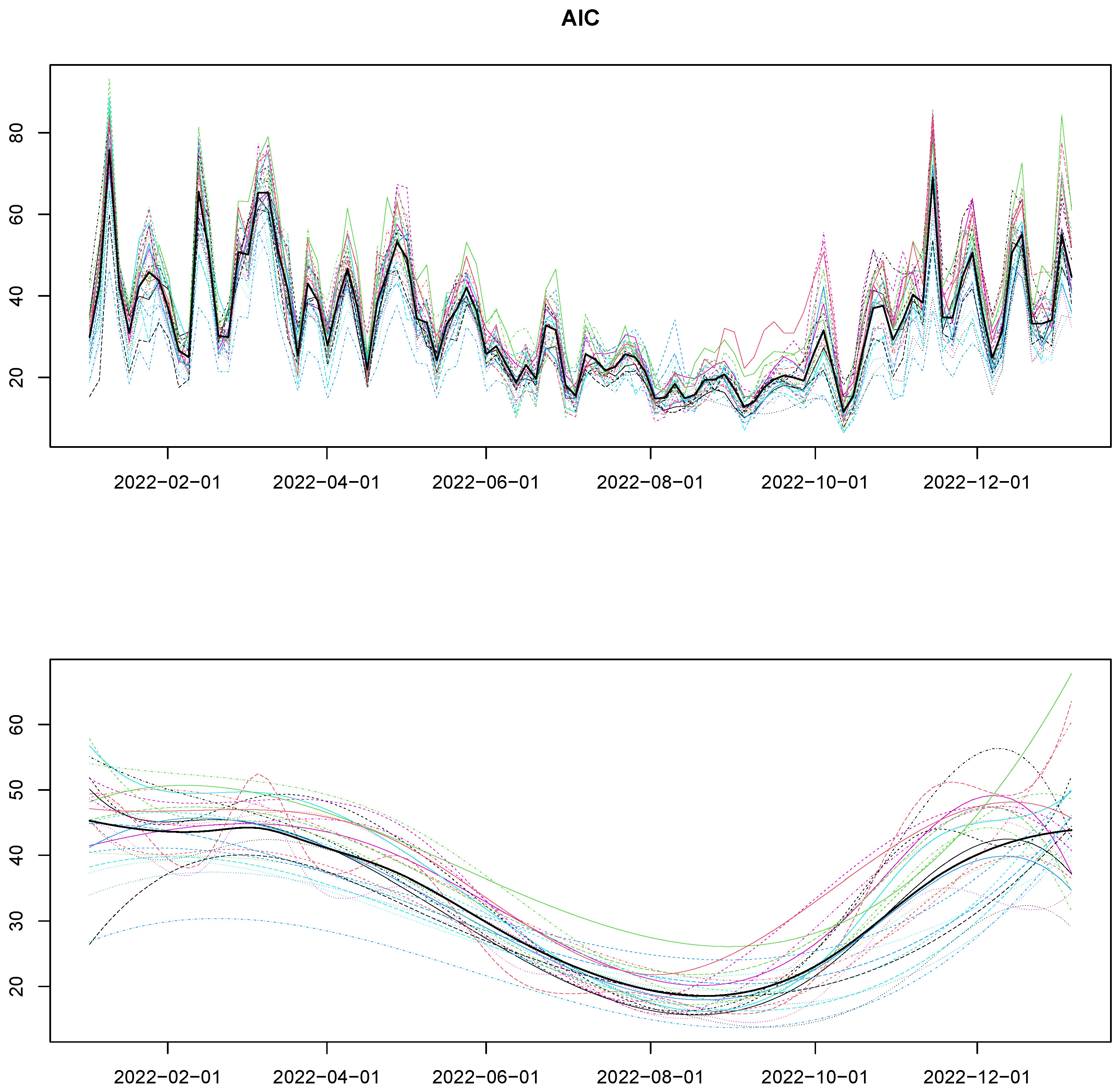
The raw daily values were then converted to smooth functional trajectories using cubic B-spline bases combined with penalized smoothing. The choice of smoothing parameter was determined by comparing the Akaike information criterion (AIC) and the Bayesian information criterion (BIC). Supplemental Figures S4 and S5 illustrate the effect of these two criteria. In general, AIC allows for greater local flexibility, thereby preserving episodic peaks that may be environmentally meaningful, whereas BIC imposes stronger regularization and occasionally suppresses such structure, particularly at stations with relatively low variability. Considering this behavior, subsequent analyses were conducted using AIC-based smoothed curves. Figure 4 displays the collection of smoothed curves for all stations, together with their corresponding mean functions.

Figure 4. Functional curves for all stations under AIC (top panel) and BIC (bottom panel) criteria, with mean curves shown in black.

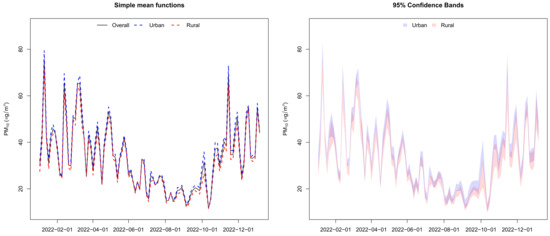
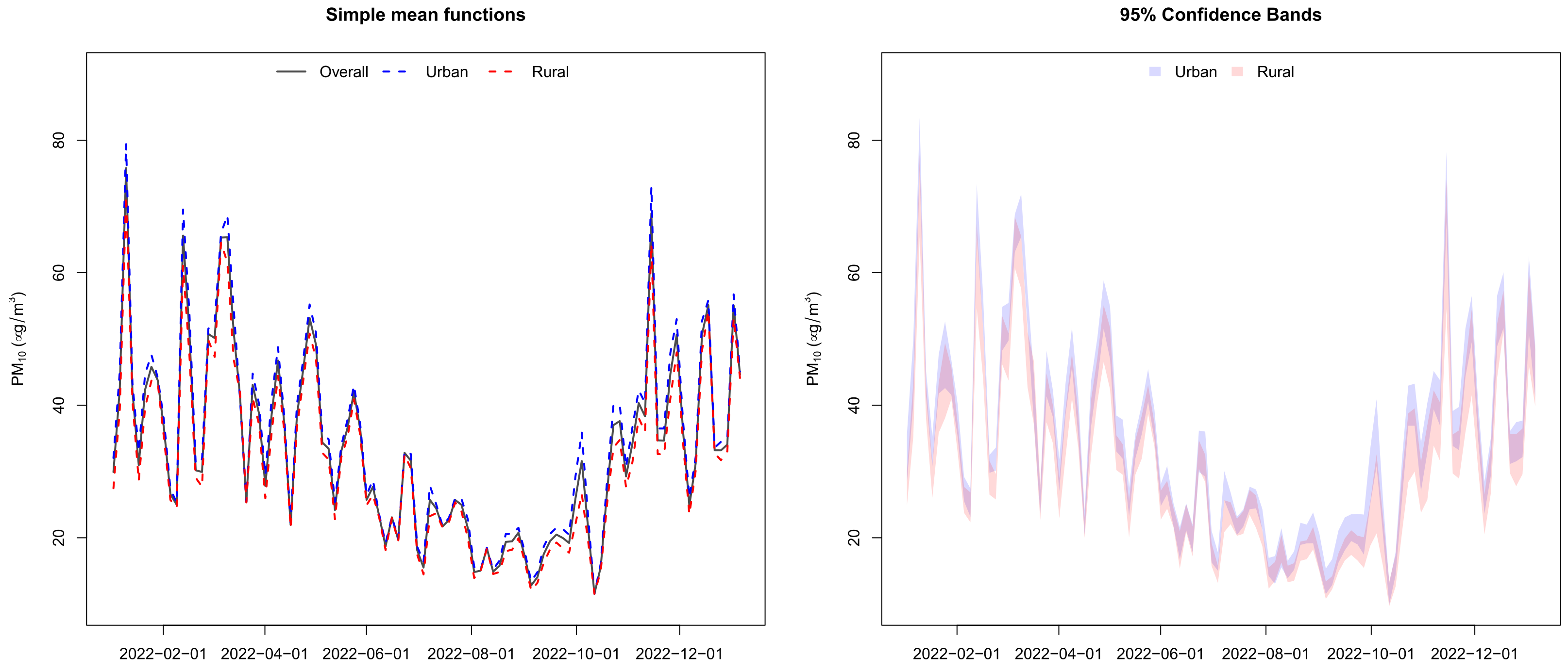
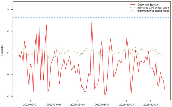
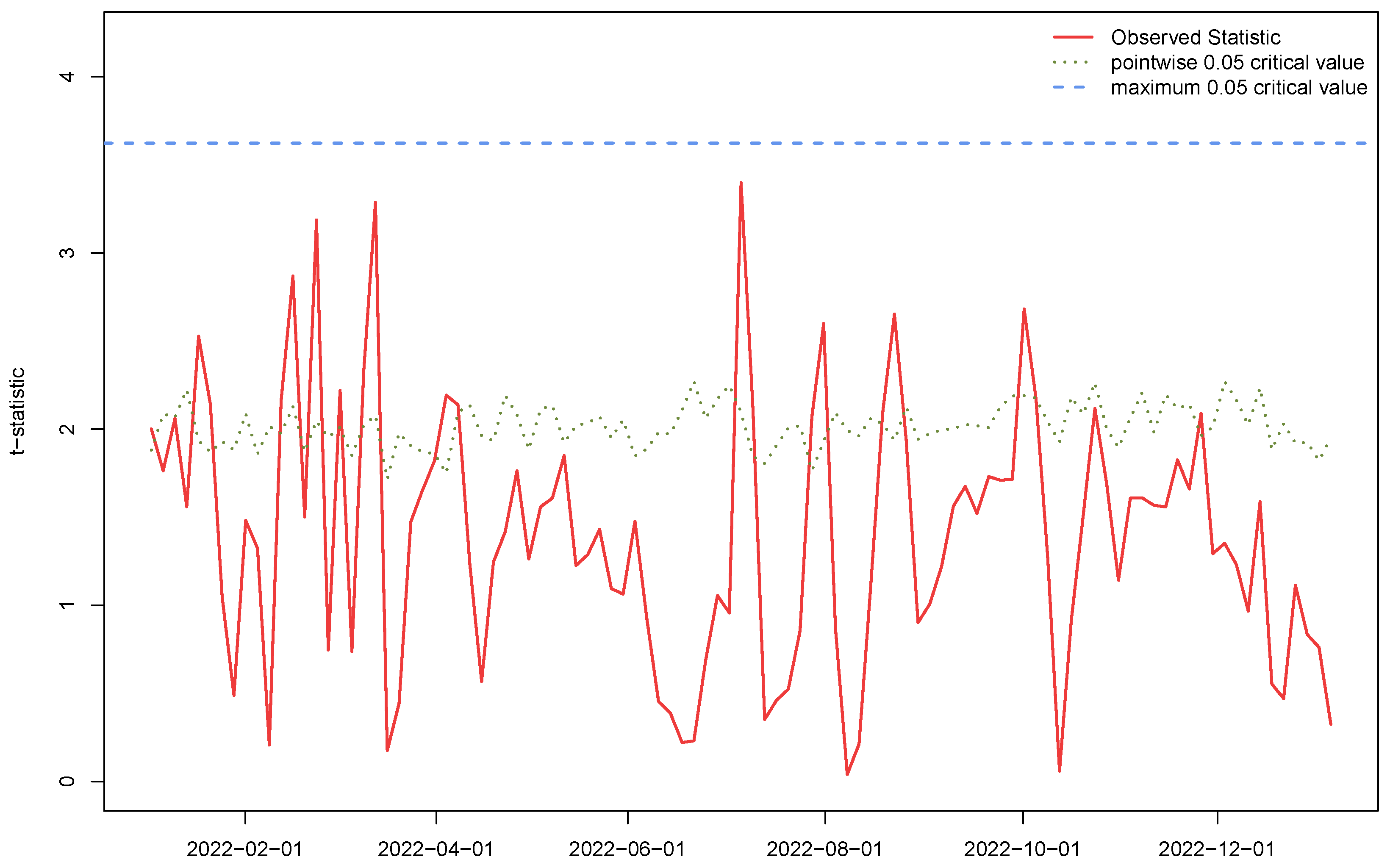
Visual inspection of the sample mean functions in Figure 5 (left panel) suggests that urban stations tend to maintain higher levels than the provincial mean, while rural stations remain slightly below it. This pattern may reflect the influence of traffic and industrial emissions, which are generally higher in urban regions. However, to formally examine whether these apparent differences are statistically meaningful, a permutation-based functional two-sample t-test was implemented. The resulting test statistic is plotted in Figure 6. Although pointwise values occasionally exceed critical thresholds during certain time intervals, the global maximum statistic—used as the formal decision criterion—does not surpass the permutation-based critical value. This indicates that, despite the apparent differences in the mean curves shown in Figure 5 (left panel), the largely overlapping 95% confidence bands in Figure 5 (right panel) suggest that the patterns observed in the mean curves are not statistically significant.

Figure 5. Sample mean functions (left panel): overall (solid), urban (blue dashed), rural (red dashed). 95% confidence bands (right panel): urban (blue) and rural (red).

Figure 6. Functional two-sample t-test comparing urban and rural mean functions.

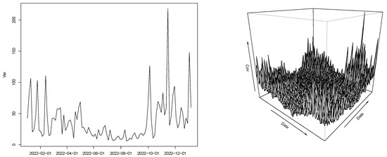
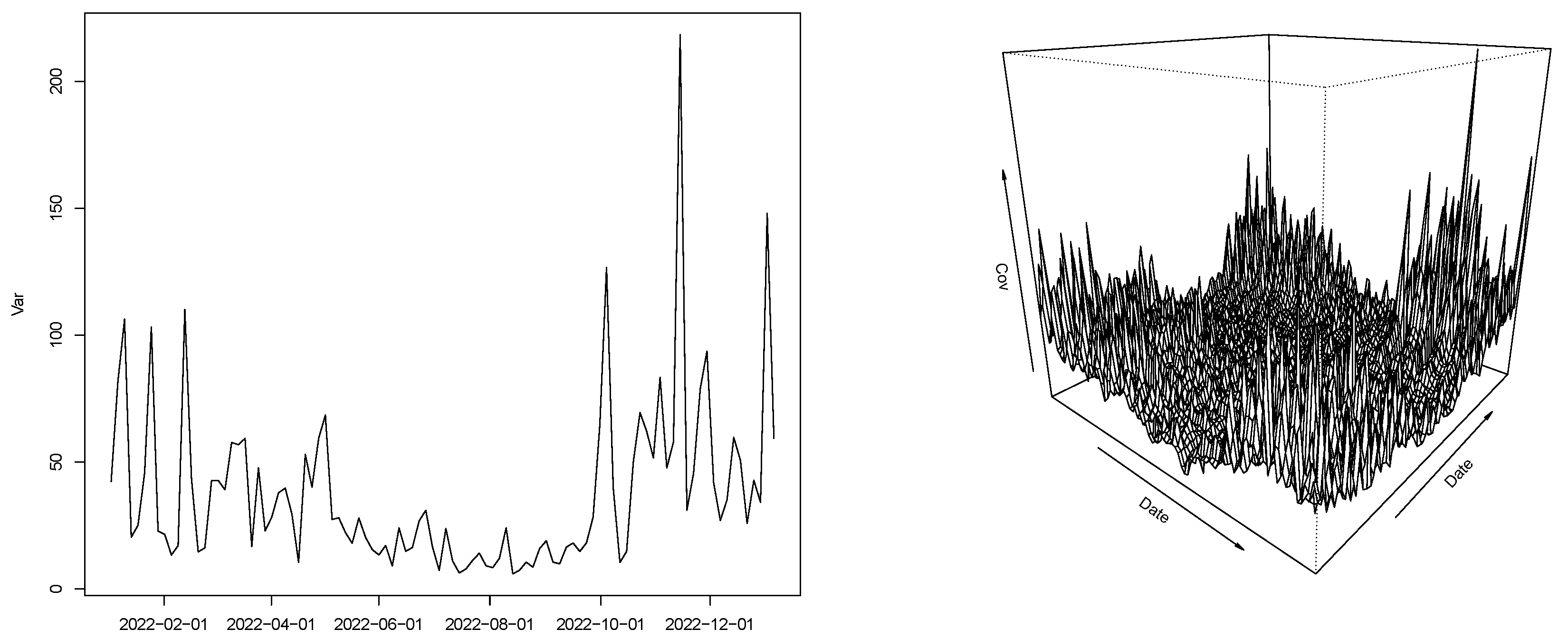
Further insight into temporal variability was obtained by examining the estimated variance function and covariance surface, shown in Figure 7. Variance is largest from late winter through spring and again in late autumn, indicating that inter-station variability is driven primarily by periods in which abrupt changes occur. Outside these intervals, temporal dependence is relatively weak, consistent with the smoother summer trajectories.

Figure 7. Variance function (left panel) and covariance surface (right panel) of PM₁₀ functional curves.

Finally, FPCA was applied to the smoothed curves in order to extract the main modes of variation. Supplemental Figure S6 presents the first four principal components, along with the mean curve and corresponding perturbations. The first component, which explains 58.4% of the total variation, reflects overall elevation of pollution concentrations, particularly during winter and early spring. The second component, accounting for 10.6%, captures contrasts within the winter season, highlighting differing magnitudes of peak intensity. The third component (7.7%) is associated with fluctuations concentrated in May and June, while the fourth component (5.5%) represents relatively small deviations around the summer minimum. For comparison, FPCA based on BIC-smoothed curves (Supplemental Figure S7) yielded a similar set of principal components but with a reduced proportion of variance explained by the leading modes (58.4%, 10.6%, 7.7%, and 5.5% for PC1–PC4), reflecting the stronger regularization imposed by BIC. Because the primary goal of this study is to characterize temporal patterns and variability in daily PM₁₀ concentrations, preserving such variability is essential; therefore, AIC-based smoothing was adopted for all subsequent functional analyses. Together, these components provide a concise but informative summary of the temporal structure underlying PM₁₀ dynamics in Chungbuk and form the basis for interpretation in the subsequent discussion.

To further explore spatial heterogeneity, FPCA scores were compared between urban and rural stations (Supplemental Figure S8; Supplemental Table S1). For PC1 (overall pollution level), urban stations exhibit substantially higher median scores than rural stations, indicating generally elevated PM₁₀ trajectories in urban areas. PC2 (seasonal deviations, particularly winter peaks) shows some differences in range and distribution between groups, with a few urban stations displaying low scores, reflecting localized variability, and lower median and mean and slightly larger standard deviation in urban stations. PC3 (late spring fluctuations) includes a few outliers in the urban group, but median scores are similar across groups, with mean and standard deviation comparable across groups, suggesting limited contribution to group-level differences. PC4 (minor summer deviations) shows largely overlapping distributions, indicating that this mode primarily reflects individual station-specific patterns rather than systematic group differences. Importantly, although PC3 and PC4 exhibit some variability across stations, formal statistical testing did not detect significant differences between urban and rural groups for these components. Together, these results indicate that the main regional differences are captured in PC1 and PC2, while PC3 and PC4 largely contextualize the null result from the formal functional two-sample test, confirming that overall temporal trajectories are broadly similar across urban and rural sites.

5. Discussion and Conclusions

This study applied a functional data analysis framework to daily PM₁₀ concentrations collected from 28 atmospheric monitoring stations in Chungcheongbuk-do (Chungbuk), Korea. By representing each monitoring record as a smooth functional curve, we were able to examine seasonal behavior, assess potential differences between urban and rural regions, and summarize dominant temporal patterns through functional principal component analysis (FPCA). Viewing the pollution series as continuous trajectories rather than discrete observations provided a unified lens through which the temporal evolution of air quality could be interpreted in a more coherent and informative manner.

The empirical results revealed a pronounced seasonal cycle consistent with prior domestic and international findings. Concentrations were highest during late winter and early spring, declined markedly during the summer months, and increased again toward late autumn. The mean curve showed several short-lived but substantial surges, particularly in January–March, May, and November, indicating episodic events that likely reflect interactions among meteorological conditions, local emissions, and transported pollutants. When stations were partitioned into urban and rural groups, descriptive comparisons suggested somewhat elevated levels in urban locations throughout much of the year. Nevertheless, the permutation-based functional t-test indicated that these differences were not statistically significant once the full temporal profile was considered. This finding suggests that regional background influences may exert a strong homogenizing effect, reducing contrasts that might otherwise arise solely from local urbanization or traffic-related sources. Such an interpretation is broadly consistent with earlier studies highlighting the role of large-scale transport and synoptic weather patterns in shaping particulate dynamics.

FPCA offered an interpretable decomposition of temporal variability. The first principal component, explaining more than half of the total variation, primarily captured the overall level of pollution and its pronounced elevation during winter and early spring. Subsequent components isolated more localized phenomena, including contrasts within the winter period, variability concentrated in late spring, and subtle fluctuations around summer minima. Together, these components constitute a compact set of indices that summarize seasonal structure in a manner that is both statistically efficient and substantively meaningful. They also provide a natural foundation for future work that may seek to link temporal features of PM₁₀ to meteorological covariates, emission sources, or health outcomes.

From a methodological perspective, the analysis illustrates how FDA can complement traditional time-series approaches. Representing the data as curves allows for the preservation of continuous-time information and avoids the need to focus exclusively on isolated time points or summary averages. The penalized B-spline estimator with total variation penalty proved particularly effective in balancing smoothness with the ability to capture episodic peaks, thereby reducing the likelihood of oversmoothing features that may hold environmental significance. Functional hypothesis testing enabled global comparison of temporal patterns across groups, while FPCA exposed low-dimensional structure that can be readily interpreted and incorporated into subsequent modeling efforts. Rather than replacing existing regression or spatio-temporal frameworks, FDA provides additional structure that can be combined with them to improve interpretability and, potentially, predictive accuracy.

The findings also carry several practical implications. The absence of a statistically significant distinction between urban and rural curves implies that mitigation strategies focused exclusively on urban centers may overlook broader regional drivers. Coordinated provincial policies, early-warning systems tailored to seasonal peaks, and public risk communication strategies may therefore be more effective than measures targeted only at specific cities. Moreover, FPCA-derived scores could be used as concise indicators of abnormal seasonal behavior, enabling earlier identification of periods in which unusually severe winter or spring pollution is developing. These results provide practical guidance for environmental monitoring agencies: the identification of dominant temporal patterns and seasonal deviations can help optimize monitoring station placement, support long-term trend analysis, and inform early warning and public communication strategies.

At the same time, several limitations warrant consideration. The analysis was restricted to a single year (2022), limiting the ability to evaluate long-term structural changes or policy effects across multiple years. Meteorological factors and co-pollutants, which are known to influence PM dynamics, were not explicitly included in the current modeling framework. As a result, the identified temporal patterns should be interpreted as descriptive characteristics of PM₁₀ variability rather than as evidence of causal relationships, and any policy or environmental implications should be considered with appropriate caution. Importantly, these limitations may influence the FPCA and functional test results. Because the analysis is restricted to a single year, unusual day-to-day variability or rare events could disproportionately affect seasonal components (PC2–PC4), and the absence of meteorological covariates may lead to slight overestimation of short-term variability. Overall, the main temporal patterns appear robust, but specific components may be sensitive to single-year anomalies or unmeasured confounding factors. In addition, smoothing parameters were selected using information criteria; alternative procedures such as cross-validation or Bayesian methods may provide different perspectives on uncertainty and model selection. Addressing these issues in future work would enhance the robustness of conclusions and yield a more comprehensive picture of pollution dynamics.

Looking ahead, several natural extensions emerge. Functional regression models could be employed to relate PM₁₀ curves to meteorological drivers or health indicators, offering a more explicit link between exposure trajectories and outcomes. Spatio-functional approaches would allow for joint modeling of temporal curves across monitoring locations, capturing both spatial correlation and temporal evolution. Extending the framework to multiple pollutants would facilitate analysis of joint exposure processes. Specially, extending FDA to multi-year data using a year-as-function approach could capture inter-annual variability and long-term trends, providing further insight into temporal stability and episodic events across years. These directions collectively underline the versatility of FDA as a tool for environmental monitoring and public-health assessment.

In conclusion, the study demonstrates that functional data analysis provides a powerful and insightful approach for investigating the temporal behavior of PM₁₀ concentrations in Chungbuk. By combining penalized spline smoothing, functional hypothesis testing, and FPCA, we obtained a parsimonious yet detailed representation of seasonal variation, episodic peaks, and between-station heterogeneity. As air pollution monitoring networks continue to expand and data become more granular, the functional perspective is likely to assume an increasingly important role in statistical analyses that inform environmental policy and health-related decision-making.

References

- Ramsay, J.O.; Silverman, B.W. Functional Data Analysis, 2nd ed.; Springer Series in Statistics; Springer: New York, NY, USA, 2005. [Google Scholar] [CrossRef] [Scilit]
- Ramsay, J.O.; Hooker, G.; Graves, S. Functional Data Analysis with R and MATLAB; Use R! Springer: New York, NY, USA, 2009. [Google Scholar] [CrossRef] [Scilit]
- Aneiros, G.; Horová, I.; Hušková, M.; Vieu, P. On functional data analysis and related topics. J. Multivar. Anal. 2022, 189, 104861. [Google Scholar] [CrossRef] [Scilit]
- Jhong, J.H.; Koo, J.Y.; Lee, S.W. Penalized B-spline estimator for regression functions using total variation penalty. J. Stat. Plan. Inference 2017, 184, 77–93. [Google Scholar] [CrossRef] [Scilit]
- Jang, A.S. Impact of particulate matter on health. J. Korean Med Assoc. 2014, 57, 763–768. [Google Scholar] [CrossRef] [Scilit]
- International Agency for Research on Cancer. Outdoor Air Pollution a Leading Environmental Cause of Cancer Deaths. Press Release No. 221. 2013. Available online: https://www.iarc.who.int/wp-content/uploads/2018/07/pr221_E.pdf (accessed on 5 February 2023).
- World Health Organization. WHO Global Air Quality Guidelines: Particulate Matter (PM2.5 and PM10), Ozone, Nitrogen Dioxide, Sulfur Dioxide and Carbon Monoxide; World Health Organization: Geneva, Switzerland, 2021; Available online: https://www.who.int/publications/i/item/9789240034228 (accessed on 5 February 2023).
- Hoffmann, B.; Boogaard, H.; de Nazelle, A.; Andersen, Z.J.; Abramson, M.; Brauer, M.; Brunekreef, B.; Forastiere, F.; Huang, W.; Kan, H.; et al. WHO Air Quality Guidelines 2021–Aiming for healthier air for all: A joint statement by medical, public health, scientific societies and patient representative organisations. Int. J. Public Health 2021, 66, 1604465. [Google Scholar] [CrossRef] [Scilit] [PubMed]
- Yeo, M.J.; Kim, Y.P. Trends of the PM10 concentrations and high PM10 concentration cases in Korea. J. Korean Soc. Atmos. Environ. 2019, 35, 249–264. [Google Scholar] [CrossRef] [Scilit]
- Lee, J.; Lee, S. Analysis of the current state of fine dust and pollution sources in Chungcheongbuk-do. J. Inst. Constr. Technol. 2021, 40, 35–43. (In Korean) [Google Scholar]
- Allabakash, S.; Lim, S.; Chong, K.S.; Yamada, T.J. Particulate matter concentrations over South Korea: Impact of meteorology and other pollutants. Remote Sens. 2022, 14, 4849. [Google Scholar] [CrossRef] [Scilit]
- Kim, J.M. Copula dynamic conditional correlation and functional principal component analysis of COVID-19 mortality in the United States. Axioms 2022, 11, 619. [Google Scholar] [CrossRef] [Scilit]
- Dominici, F.; McDermott, A.; Zeger, S.L.; Samet, J.M. On the use of generalized additive models in time-series studies of air pollution and health. Am. J. Epidemiol. 2002, 156, 193–203. [Google Scholar] [CrossRef] [Scilit] [PubMed]
- Cameletti, M.; Lindgren, F.; Simpson, D.; Rue, H. Spatio-temporal modeling of particulate matter concentration through the SPDE approach. AStA Adv. Stat. Anal. 2013, 97, 109–131. [Google Scholar] [CrossRef] [Scilit]
- Morris, J.S. Functional regression. Annu. Rev. Stat. Its Appl. 2015, 2, 321–359. [Google Scholar] [CrossRef] [Scilit]
- De Boor, C. A Practical Guide to Splines; Springer: New York, NY, USA, 1978. [Google Scholar]
- Liu, X.; Yang, L.; Chen, L. Functional time series modeling with dependence: A survey. Axioms 2023, 12, 433. [Google Scholar] [CrossRef] [Scilit]
- Bozdogan, H. Model selection and Akaike’s information criterion (AIC): The general theory and its analytical extensions. Psychometrika 1987, 52, 345–370. [Google Scholar] [CrossRef] [Scilit]
- Schwarz, G. Estimating the dimension of a model. Ann. Stat. 1978, 6, 461–464. [Google Scholar] [CrossRef] [Scilit]
Disclaimer/Publisher’s Note: The statements, opinions and data contained in all publications are solely those of the individual author(s) and contributor(s) and not of MDPI and/or the editor(s). MDPI and/or the editor(s) disclaim responsibility for any injury to people or property resulting from any ideas, methods, instructions or products referred to in the content. |
© 2026 by the authors. Licensee MDPI, Basel, Switzerland. This article is an open access article distributed under the terms and conditions of the Creative Commons Attribution (CC BY) license.