Expected Maximization of a Concave Utility Function Under Threshold-Based Activation

Abstract

Maximizing the expected value of a concave and strictly increasing utility function defines a fundamental class of discrete optimization problems. Among them, coverage decision problems with diminishing marginal returns under uncertainty, typically modeled via a set-union operator, have been extensively studied. In the classical framework, an item becomes active once it is covered by at least one chosen meta-item. Motivated by increasing robustness requirements in applications such as automated systems, social networks, and emergency response planning, we extend this setting by introducing threshold-based activation. The resulting generalized problem can be formulated as a mixed-integer nonlinear programming problem, for which we further propose three exact algorithms. The first two methods linearize the utility function using submodular cuts (SC) and outer-approximation (OA) techniques, respectively, resulting in formulations that can be solved exactly by off-the-shelf mixed-integer linear programming solvers. The third method builds upon the OA framework and further employs Benders decomposition (BD) to project out the item-related variables, which enables superior performance on ultra-large-scale instances. Extensive computational experiments show that, compared with the SC and BD methods, the OA method exhibits a substantial speed advantage on instances with a size of around 40,000, which can be solved within 100 s. In contrast, for ultra-large-scale instances with more than 100,000 items, the BD method demonstrates superior computational efficiency. These results provide practical guidance for algorithmic strategy selection and further demonstrate the computational tractability of this broader class of utility maximization problems under threshold-based activation.

1. Introduction

The problem of maximizing the expected value of a concave, strictly increasing, and differentiable utility function f applied to the aggregate value of a selected item set has been extensively studied in the literature [1,2,3]. Such utility functions naturally capture diminishing marginal returns while preserving monotonicity, reflecting the intuitive principle that additional resources always increase utility but at a decreasing rate [4]. A commonly adopted specification is $f\left(z\right)=1-exp(-z/\lambda )$, where $\lambda >0$ controls the degree of concavity and thus the level of risk aversion. To formalize this class of problems, a finite ground set of items J is given, and uncertainty is modeled through a finite set of scenarios K, where each scenario $k\in K$ is associated with a value vector ${\mathit{a}}_k={\left(a_{kj}\right)}_{j\in J}$. Let $\mathcal{X}\subseteq 2^J$ denote the family of all feasible selections. The objective is to select a subset $S\in \mathcal{X}$ that maximizes the expected utility:

$$\underset{S\in \mathcal{X}}{max}\sum _{k\in K}{\pi }_{k}f\left(\sum _{j\in S}{a}_{kj}+d_k\right).$$

(1)

Here, ${\pi }_k$ denotes the probability of scenario k and $d_k$ is a scenario-dependent constant. This class of problems has found wide applicability across multiple domains, including expected utility theory [4], facility location [5], and combinatorial auctions [6].

More recently, Coniglio et al. [7] generalized this framework by replacing the additive structure with a set-union operator. In the resulting model, a set of meta-items I is introduced, where each meta-item $i\in I$ covers a subset $S_i\subseteq J$ of the ground set. Let $\mathcal{Y}\subseteq 2^I$ denote the family of all feasible selections of meta-items. The decision problem is to select a subset of meta-items $T\in \mathcal{Y}$ so as to maximize the utility, which is evaluated on the activated items, defined as the union of the item covered by the selected meta-items, namely, $S={\bigcup }_{i\in T}{S}_i$:

$$\underset{T\subseteq \mathcal{Y}}{max}\sum _{k\in K}{\pi }_{k}f\left(\sum _{j\in {\bigcup }_{i\in T}{S}_i}{a}_{kj}+d_k\right).$$

(2)

This set-union-based framework admits a natural interpretation in influence maximization problems in social networks [8]. In this context, the ground set J represents the set of users in the network, while set I corresponds to candidate seed users. A selected seed user i activates a subset of users $S_i\subseteq J$ that can be influenced by i. Accordingly, for a selected seed user set $T\subseteq I$, the resulting activated user set is given by ${\bigcup }_{i\in T}{S}_i$. The expected activation utility can then be expressed as ${\sum }_{k\in K}{\pi }_{k}f\left({\sum }_{j\in {\bigcup }_{i\in T}{S}_i}{a}_{kj}\right)$, where ${\pi }_k$ denotes the probability of scenario k, $a_{kj}$ represents the weight or utility of user j in scenario k, and f is the utility function. This formulation reveals that influence maximization can be viewed as a stochastic set-covering problem, in which the set-union operator captures the cumulative coverage of activated users and naturally induces a submodular objective function. Additionally, this modeling framework also arises in marketing problems [9] and stochastic competitive facility location [10].

In this paper, we further generalize this problem by introducing activation thresholds for items in the ground set, whereby an item is activated only when it is covered by many sufficiently selected meta-items. Specifically, for each item $j\in J$, let $M_j\in {\mathbb{Z}}_{+}$ denote its activation threshold. Given a selected subset $T\subseteq I$, item j is activated if and only if $\left|I\left(j\right)\cap T\right|\ge M_j$, where $I\left(j\right)$ is the set of meta-items that cover item j. Accordingly, the item set activated by T is defined as $S\left(T\right)=\left\{j\in J:\left|I\left(j\right)\cap T\right|\ge M_j\right\}$, and the corresponding decision problem can be formulated as

$$\underset{T\subseteq I}{max}\sum _{k\in K}{\pi }_{k}f\left(\sum _{j\in S\left(T\right)}{a}_{kj}+d_k\right).$$

(3)

Under this generalized activation rule, the activated set $S\left(T\right)$ is no longer determined by a simple set union, but instead by these threshold-based activation constraints. When $M_j=1$ for all $j\in J$, the proposed model reduces to the classical set-union formulation studied in Coniglio et al. [7], demonstrating that our framework strictly generalizes existing models. When the utility function $f(·)$ is linear, model (3) reduces to the Maximal Availability Location Problem (MALP) [11,12], which has been extensively studied in the facility location literature. A closely related formulation is the (PSMCP) [13,14], in which activation thresholds are similarly imposed on items, and the objective is to select the minimum number of sets such that the total covered utility exceeds a prescribed target level. Variants of MALP and PSMCP have been widely investigated in the combinatorial optimization literature [15,16,17,18,19,20]. However, the linear utility structure adopted in these formulations limits their ability to capture diminishing marginal returns and heterogeneous valuation effects that frequently arise in practice. For example, in social network applications, the value of activating a user may depend on multiple dimensions, such as purchasing power, influence, and engagement intensity, which cannot be adequately represented by a simple linear aggregation [21,22,23]. By incorporating a concave utility function into the objective, our framework can be viewed as a generalization of both MALP and PSMCP. It enables a richer representation of nonlinear benefit structures under budget constraints, whose practical implications are discussed in greater detail below.

More broadly, a wide range of real-world applications can be naturally modeled within this threshold-based activation framework. A prominent example arises in cumulative activation processes in social networks [24]. Most existing studies on influence maximization focus on one-shot propagation mechanisms in which influence is propagated from seed users only once according to a probabilistic diffusion model. However, in many practical settings, a single exposure is often insufficient to trigger adoption. Instead, influence accumulates over multiple rounds of information dissemination until a user’s internal adoption threshold is reached. Moreover, users exhibit heterogeneous susceptibility to influence: some may be easily activated after a few exposures, while others require repeated reinforcement. Such multi-round propagation mechanisms more accurately capture the cumulative nature of influence diffusion in real social networks. For instance, an empirical study on Twitter by Romero et al. [25] shows that the probability of adopting a hashtag increases significantly with the number of exposures, typically reaching its peak after two to four exposures rather than after the first one. Within our threshold-based activation framework, $I\left(j\right)\subseteq I$ represents the set of seed users that can influence user j. Given a set of selected seed users $T\subseteq I$, a user $j\in J$ becomes activated only if the number of seed users in T influencing j reaches or exceeds its activation threshold $M_j$, i.e., $\left|I\left(j\right)\cap T\right|\ge M_j$.

Another important application arises in stochastic facility location problems, which involve a set of customers J and a set of potential facility locations I. The objective is to select a subset of facilities $T\subseteq I$ to maximize the expected satisfied demand under multicover constraints, which naturally arise in settings where reliable coverage requires redundancy [11,12,26]. In practice, reliability considerations often require each demand point to be covered by at least two facilities to ensure service continuity under single-facility failure scenarios, such as disruptions caused by adverse weather or operational breakdowns [27]. Multicover requirements can be modeled by introducing activation thresholds $M_j\in {\mathbb{Z}}_{+}$ for each customer $j\in J$, such that customer j belongs to the activated set $S\left(T\right)$ only if at least $M_j$ selected facilities cover it. In the stochastic setting, the expected utility of a facility selection T can be expressed as ${\sum }_{k\in K}{\pi }_{k}f\left({\sum }_{j\in S\left(T\right)}{a}_{kj}\right)$, where K denotes a set of possible demand scenarios (e.g., weekdays and holidays exhibiting different traffic patterns for wireless towers), $a_{kj}$ represents the demand of customer j in scenario k, and ${\pi }_k$ is the probability of scenario k.

A third class of applications arises in marketing problems, where firms aim to select a subset of products or advertising channels to maximize the number of consumers who form brand awareness. In typical marketing settings, customer loyalty or sustained engagement is often not established by exposure to a single product or advertisement alone. Instead, effective engagement commonly requires repeated or simultaneous exposure to multiple marketing stimuli from the same brand, reflecting a cumulative persuasion effect [28,29]. Empirical evidence in advertising practice suggests that approximately three exposures within a purchase cycle constitute a baseline level for achieving persuasive impact [30]. This phenomenon can be naturally modeled through a threshold-based mechanism, in which a consumer segment j becomes effectively engaged only when the number of attractive products or advertisements associated with the same brand exceeds a segment-specific threshold $M_j$. In media planning settings, a closely related concept is effective frequency, which refers to the minimum number of advertising exposures required for a consumer j to be effectively influenced, thus naturally corresponding to the threshold $M_j$. Early studies suggest that repeated advertising exposure is necessary for effectiveness, with Naples identifying three exposures within a purchase cycle as a baseline level of effective frequency [30]. Ostrow proposes that this effective frequency threshold should be adjusted according to target audiences and market conditions [31]. More recent empirical evidence indicates that, particularly in local markets with limited budgets, planners tend to prioritize frequency over reach while still relying on the effective frequency principle adapted to market-specific conditions [32].

By introducing binary decision variables, Problem (1) can be formulated as a mixed-integer nonlinear programming (MINLP) problem, which is described in detail in the next section. Since in Problem (1) all coefficients $a_{kj}$ and $d_k$ are nonnegative and the utility function f is concave and nondecreasing, this problem can be naturally viewed as a submodular function maximization problem, which is known to be NP-hard [33]. A standard method to address such problems is to linearize the submodular function via submodular cuts [34], so that Problem (1) can be reformulated as a mixed-integer linear programming (MILP) for exact solution. Building on this formulation, Ahmed and Atamtürk [1] conducted a polyhedral analysis of this class of MILPs and applied lifting techniques to significantly strengthen the standard submodular formulation. Subsequently, Yu and Ahmed [2] further investigated the variant of the problem with a single knapsack constraint. Shi et al. [35] extended the results of Ahmed and Atamtürk [1] and studied the case involving multiple disjoint cardinality constraints. For Problem (2), Coniglio et al. [7] employed outer-approximation, Benders decomposition, and submodular cuts methods to linearize both the submodular objective function and the set-union operator, and provided a comparative evaluation of the resulting formulations. Subsequently, Lamontagne et al. [36] studied a dynamic (multi-period) variant of this problem and developed an exact solution method using Benders decomposition. Despite the wide range of practical applications and the growing demand for Problem (3), effective exact solution methods for these generalized models remain largely underdeveloped.

To address this gap, this paper studies Problem (3) and develops exact solution algorithms, with particular emphasis on instances in which the number of items exceeds the number of meta-items. The main contributions of this work are summarized as follows:

• We generalize the framework of Problem (2) by relaxing the single-coverage assumption, allowing an item to be considered activated only when it is simultaneously covered by a prescribed threshold. The resulting formulation broadens the applicability of the framework to settings such as social influence propagation, stochastic facility location, marketing and media planning.
• Three exact algorithms are proposed. The first algorithm is based on direct linearization by submodular cut (SC) method. The second algorithm relies on a single hypograph formulation using outer approximation (OA) method. Building on the OA framework, a third algorithm further incorporates Benders decomposition (BD) method to project out item-related variables, thereby substantially enhancing scalability on very large-scale instances. These methods offer practical solution choices for real-world applications.
• Extensive numerical experiments were conducted to evaluate the performance of the three methods. The results indicate that the OA method can solve instances with a size of up to 40,000 within 100 s, achieving solution times that are approximately 2–5 times faster than those of the BD method. In contrast, for very large-scale instances with more than 100,000 items, the BD method exhibits superior performance and outperforms the OA method. Overall, the SC method generally performs worse than the other two methods.

The remainder of this paper is organized as follows. Section 2 formally presents a MINLP formulation. Section 3 develops three exact solution methods for the proposed problem. Section 4 describes in detail the branch-and-cut implementation framework, including the separation strategies and pseudocode for each method. Section 5 reports extensive computational experiments, compares the performance of the three methods, and provides a detailed analysis of the numerical results. Section 6 summarizes the main contributions and findings of this paper and discusses directions for future research.

2. Problem Formulation

In this section, we formally present the mathematical formulation of the problem. Let the binary vector $\mathit{x}\in {\{0,1\}}^{\left|J\right|}$ indicate whether each item is activated. Specifically, for each $j\in J$, $x_j=1$ if $j\in \mathcal{X}$, and $x_j=0$ otherwise. Problem (1) can then be equivalently written as

$$\begin{array}{cc}\hfill \underset{\mathit{x}}{max}& \sum _{k\in K}{\pi }_{k}f\left(\sum _{j\in J}{a}_{kj}{x}_j+d_k\right)\hfill \end{array}$$

(4a)

$$\begin{array}{cc}\hfill \mathrm{s}.\mathrm{t}.& \mathit{x}\in X,\hfill \end{array}$$

(4b)

$$\begin{array}{cc}\hfill & \mathit{x}\in {\{0,1\}}^{\left|J\right|},\hfill \end{array}$$

(4c)

where $X\subseteq {\{0,1\}}^{\left|J\right|}$ denotes the feasible region of decision vector $\mathit{x}$. The objective function (4a) maximizes the expected utility across all scenarios, where the utility in each scenario $k\in K$ is evaluated based on the total value of the activated items.

Furthermore, we introduce a binary decision variable $\mathit{y}\in {\{0,1\}}^{\left|I\right|}$ to indicate whether meta-item $i\in I$ is selected. An item $j\in J$ becomes activated (i.e., $x_j=1$) if and only if at least one meta-item in set $I\left(j\right)$ is selected. This covering condition is encoded by the constraints

$$\begin{array}{cc}\hfill x_j& \le \sum _{i\in I\left(j\right)}{y}_i,\forall j\in J,\hfill \end{array}$$

(5a)

$$\begin{array}{cc}\hfill y_i& \le x_j,\forall i\in I\left(j\right),j\in J.\hfill \end{array}$$

(5b)

Building on this structure, Problem (2) can be formulated as the following MINLP:

$$\begin{array}{cc}\hfill \underset{\mathit{x},\mathit{y}}{max}& \sum _{k\in K}{\pi }_{k}f\left(\sum _{j\in J}{a}_{kj}{x}_j+d_k\right)\hfill \\ \hfill \mathrm{s}.\mathrm{t}.& \left(4\mathrm{c}\right),\left(5\mathrm{a}\right),\left(5\mathrm{b}\right)\hfill \end{array}$$

(6a)

$$\begin{array}{cc}\hfill & \mathit{y}\in Y,\hfill \end{array}$$

(6b)

$$\begin{array}{cc}\hfill & \mathit{y}\in {\{0,1\}}^{\left|I\right|},\hfill \end{array}$$

(6c)

where $Y\subseteq {\{0,1\}}^{\left|I\right|}$ denotes the feasible region of decision vector $\mathit{y}$, such as those induced by budget constraints ${\sum }_{i\in I}{b}_i{y}_i\le B$, with $(\mathit{b},B)\in {\mathbb{R}}_{+}^{\left|I\right|}\times {\mathbb{R}}_{+}$, or by cardinality constraints ${\sum }_{i\in I}{y}_i\le B$, with $B\in {\mathbb{Z}}_{+}$.

In the presence of activation thresholds for items, an item $j\in J$ becomes activated (i.e., $x_j=1$) if and only if at least $M_j$ meta-items in set $I\left(j\right)$ are selected. This relationship can be enforced by the following constraints:

$$\begin{array}{cc}\hfill M_j{x}_j& \le \sum _{i\in I\left(j\right)}{y}_i,\forall j\in J,\hfill \end{array}$$

(7a)

$$\begin{array}{cc}\hfill \sum _{i\in I\left(j\right)}{y}_i& \le (M_j-1)+\left(\right|I\left(j\right)|-M_j+1)x_j,\forall j\in J.\hfill \end{array}$$

(7b)

Under this setting, Problem (3) can be equivalently reformulated as

$$\underset{\mathit{x},\mathit{y}}{max}\left\{\sum _{k\in K}{\pi }_{k}f\left(\sum _{j\in J}{a}_{kj}{x}_j+d_k\right):\left(4\mathrm{c}\right),\left(7\mathrm{a}\right),\left(7\mathrm{b}\right),\left(6\mathrm{b}\right),\left(6\mathrm{c}\right)\right\}.$$

Due to the strict monotonicity of f and the nonnegativity of $a_{kj}$, even if constraint (7b) is ignored, there exists an optimal solution in which $x_j=1$ whenever at least $M_j$ meta-items in $I\left(j\right)$ are selected. Consequently, constraints (7b) are automatically satisfied and can be omitted from the model. Hence, Problem (3) is equivalent to

$$\begin{array}{cc}\hfill \underset{\mathit{x},\mathit{y}}{max}& \sum _{k\in K}{\pi }_{k}f\left(\sum _{j\in J}{a}_{kj}{x}_j+d_k\right)\hfill \\ \hfill \mathrm{s}.\mathrm{t}.& \left(4\mathrm{c}\right),\left(7\mathrm{a}\right),\left(6\mathrm{b}\right),\left(6\mathrm{c}\right).\hfill \end{array}$$

(8)

3. Methodology

This section presents three exact solution algorithms for Problem (8). We first describe, in Section 3.1, a SC method that exploits the submodularity of the objective function to derive a MILP reformulation solvable by off-the-shelf solvers. Next, in Section 3.2, we leverage the concavity of the utility function and develop an alternative linearization based on an OA scheme. Finally, in Section 3.3, we further incorporate a BD method to project out the variables $\mathit{x}$, which enables the efficient solution of very large-scale instances.

3.1. Submodular-Cut-Based Exact Formulation

We first briefly review some useful theoretical results on SC method. Based on these results, Problem (8) is reformulated using SC method. Specifically, the nonlinear utility function is linearized, yielding a MILP formulation that can be solved by solvers.

3.1.1. Brief Review of SC Method

Let $N:=\{1,2,\dots ,n\}$ denote a finite non-empty ground set, and let $2^N:=\{S:S\subseteq N\}$ be the collection of all the subsets of N. We briefly review the fundamental theory related to submodular functions as follows.

Definition 1. 

A set function $h:2^N\to \mathbb{R}$ is submodular on N if

$$h\left(S\right)+h\left(T\right)\ge h(S\cup T)+h(S\cap T),\forall S,T\subseteq N.$$

(9)

For any subset $S\subseteq N$ and any item $i\in N\setminus S$, we define the marginal return of adding i to S as

$${\varrho }_i^h\left(S\right)=h(S\cup \left\{i\right\})-h\left(S\right).$$

(10)

Proposition 1 

([33]). The set function $h\left(S\right)$ is submodular if and only if ${\varrho }_i^h\left(S\right)\ge {\varrho }_i^h\left(T\right)$ for all $S\subseteq T\subseteq N$ and $i\in N\setminus T$.

Proposition 2 

([33]). If h is submodular, then

$$\begin{array}{cc}\hfill h\left(T\right)& \le h\left(S\right)-\sum _{j\in S\setminus T}{\varrho }_j^h(N\setminus \left\{j\right\})+\sum _{j\in T\setminus S}{\varrho }_j^h\left(S\right),S,T\subseteq N,\hfill \end{array}$$

(11)

$$\begin{array}{cc}\hfill h\left(T\right)& \le h\left(S\right)-\sum _{j\in S\setminus T}{\varrho }_j^h(S\setminus \left\{j\right\})+\sum _{j\in T\setminus S}{\varrho }_j^h(\varnothing ),S,T\subseteq N.\hfill \end{array}$$

(12)

Proposition 3 

([37]). Given a submodular function h, denote $T_{\mathit{z}}:=\{i\in N:z_i=1\}$. The following three sets are equivalent:

$$\begin{array}{cc}\hfill Q_1=& \left\{\mathit{z}\in {\{0,1\}}^n,\mu \in \mathbb{R}:\mu \le h\left(T_{\mathit{z}}\right)\right\},\hfill \\ \hfill Q_2=& \left\{\mathit{z}\in {\{0,1\}}^n,\mu \in \mathbb{R}:\mu \le h\left(S\right)-\sum _{j\in S}{\varrho }_j(N\setminus \left\{j\right\})(1-z_j)+\sum _{j\notin S}{\varrho }_j\left(S\right)z_j,\forall S\subseteq N\right\},\hfill \\ \hfill Q_3=& \left\{\mathit{z}\in {\{0,1\}}^n,\mu \in \mathbb{R}:\mu \le h\left(S\right)-\sum _{j\in S}{\varrho }_j(S\setminus \left\{j\right\})(1-z_j)+\sum _{j\notin S}{\varrho }_j(⌀)z_j,\forall S\subseteq N\right\}.\hfill \end{array}$$

3.1.2. Submodular Cut Formulation for Problem (8)

Problem (8) is equivalent to

$$\begin{array}{cc}\hfill \underset{\mathit{x},\mathit{y},\mathsf{\omega }}{max}& \sum _{k\in K}{\pi }_k{\omega }_k\hfill \end{array}$$

(13a)

$$\begin{array}{cc}\hfill \mathrm{s}.\mathrm{t}.& {\omega }_k\le h_k\left(\mathit{x}\right),\forall k\in K,\hfill \\ \hfill & \left(4\mathrm{c}\right),\left(7\mathrm{a}\right),\left(6\mathrm{b}\right),\left(6\mathrm{c}\right).\hfill \end{array}$$

(13b)

where $h_k\left(\mathit{x}\right)=f\left({\sum }_{j\in J}{a}_{kj}{x}_j+d_k\right)$ is a submodular function [1]. It follows from Propositions 2 and 3 that Problem (13) is equivalent to

$$\begin{array}{cc}\hfill \underset{\mathit{x},\mathit{y},\mathit{w}}{max}& \sum _{k\in K}{\pi }_k{\omega }_k\hfill \end{array}$$

$$\begin{array}{cc}\hfill \mathrm{s}.\mathrm{t}.& w_k\le h_k\left(X\right)+\sum _{j\in J\setminus X}{\varrho }_j^{h_k}\left(X\right)x_j-\sum _{j\in X}{\varrho }_j^{h_k}(J\setminus \left\{j\right\})(1-x_j),\forall X\subseteq J,k\in K\hfill \end{array}$$

(14a)

$$\begin{array}{cc}\hfill & w_k\le h_k\left(X\right)+\sum _{j\in J\setminus X}{\varrho }_j^{h_k}(⌀)x_j-\sum _{j\in X}{\varrho }_j^{h_k}(X\setminus \left\{j\right\})(1-x_j),\forall X\subseteq J,k\in K.\hfill \\ \hfill & \left(4\mathrm{c}\right),\left(7\mathrm{a}\right),\left(6\mathrm{b}\right),\left(6\mathrm{c}\right).\hfill \end{array}$$

(14b)

Problem (14) is a MILP and can be solved using MILP solvers based on the branch-and-bound framework. However, constraints (14a) and (14b) are exponential in number, rendering a formulation that explicitly includes all such constraints impractical. In fact, only a subset of the SCs is required to characterize an optimal solution. Therefore, we adopt the well-established branch-and-cut (B&C) framework [38,39], which solves the problem by iteratively refining a relaxed formulation that initially contains only a subset of the inequalities. Within the B&C algorithm, constraints (14a) and (14b) are treated as lazy constraints: they are not included in full at the outset; instead, only a small subset of these constraints is enforced initially, and additional violated constraints are generated and added dynamically when a candidate solution is encountered during the solution process.

At each iteration of the B&C algorithm, given a candidate solution $(\overline{\mathit{x}},\overline{\mathit{y}},\overline{\mathsf{\omega }})\in {\{0,1\}}^{\left|J\right|}\times {\{0,1\}}^{\left|I\right|}\times {\mathbb{R}}^{\left|K\right|}$, the separation problem aims to either identify a violated inequality from (14a) or (14b) or certify that no such violated inequality exists, in which case this candidate solution is feasible for the original problem. In the case of SC method, the separation procedure is straightforward: the inequality corresponding to the set $S=\{j:{\overline{x}}_j=1\}$ is violated if and only if constraint (13b) is violated.

In the B&C framework, constraints (14a) and (14b) can also be added as cutting planes. The purpose of these cutting planes is to cut off a given linear programming (LP) relaxation $(\tilde{\mathit{x}},\tilde{\mathit{y}},\tilde{\mathsf{\omega }})\in {[0,1]}^{\left|J\right|}\times {[0,1]}^{\left|I\right|}\times {\mathbb{R}}^{\left|K\right|}$ in order to strengthen the lower bound of the problem. In this case, for the separation problem, an integer solution is first obtained by rounding the fractional solution to the nearest integer. Based on this rounded integer solution, the corresponding SCs are generated, and those SCs that are violated by the LP relaxation $(\tilde{x},\tilde{y},\tilde{\omega })$ are added to the model.

Remark 1. 

Problem (8) can also be equivalently reformulated as

$$\begin{array}{cc}\hfill \underset{\mathit{x},\mathit{y},\mathsf{\omega }}{max}& \sum _{k\in K}{\pi }_k{\omega }_k\hfill \end{array}$$

(15a)

$$\begin{array}{cc}\hfill s.t.& {\omega }_k\le H_k\left(\mathit{y}\right),\forall k\in K,\hfill \\ \hfill & \left(4\mathrm{c}\right),\left(6\mathrm{b}\right),\left(6\mathrm{c}\right).\hfill \end{array}$$

(15b)

Here, $H_k\left(\mathit{y}\right)=f\left({\sum }_{j\in S}{a}_{kj}+d_k\right)$, where $S=\{j\in J:|I\left(j\right)\cap T_{\mathit{y}}|\ge M_j\}$. However, (15b) cannot be linearized using SC method because the corresponding set function $H_k\left(T_{\mathit{y}}\right)$ does not possess the submodularity property.

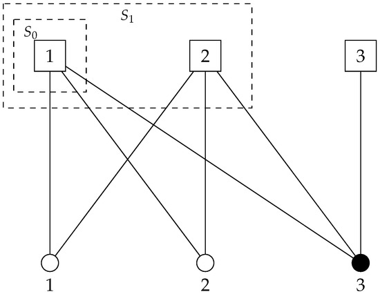
We illustrate this phenomenon through a simple example. Suppose that there are three meta-items (represented by squares) and three items (represented by circles), as shown in Figure 1. The white items require coverage from one meta-item, whereas the black items require coverage from three meta-items. Meta-items  1 and 2 are capable of covering items  1, 2, and 3, while meta-item 3 can only cover item 3. Moreover, let $f\left(x\right)=x$. Under scenario k, let $a_{kj}=1$ for all $j\in \{1,2,3\}$ and $d_k=0$. Consider the sets $S_0=\left\{1\right\}$ and $S_1=\{1,2\}$. Define

$$\mathsf{\Phi }\left(S\right)=\left\{j\in J:|I\left(j\right)\cap S|\ge M_j\right\},$$

which denotes the set of items that are activated when the selected meta-item set is S. Then we have

$$\mathsf{\Phi }\left(S_0\right)=\{1,2\},\mathsf{\Phi }\left(S_1\right)=\{1,2\},\mathsf{\Phi }(S_0\cup \left\{3\right\})=\{1,2\},\mathit{and}\mathsf{\Phi }(S_1\cup \left\{3\right\})=\{1,2,3\}.$$

Consequently,

$$H_k\left(S_0\right)=2,H_k\left(S_1\right)=2,H_k(S_0\cup \left\{3\right\})=2,\mathit{and}{H}_k(S_1\cup \left\{3\right\})=3.$$

It follows that

$${\varrho }_3^{H_k}\left(S_0\right)=H_k(S_0\cup \left\{3\right\})-H_k\left(S_0\right)=0<{\varrho }_3^{H_k}\left(S_1\right)=H_k(S_1\cup \left\{3\right\})-H_k\left(S_1\right)=1.$$

This example demonstrates that $H_k\left(T_{\mathit{y}}\right)$ violates the diminishing returns property and is therefore not submodular.

Figure 1. Illustration of non-submodularity. Squares represent meta-items, circles represent items, and dashed boxes indicate activated sets.

Let $J\left(i\right)\subseteq J$ denote the set of items covered by meta-item i. The following proposition characterizes the loss of submodularity. Without loss of generality, we assume that $f\left(x\right)=x$, $a_{kj}=1$, and $d_k=0$. Under these assumptions, for any selected set of meta-items S, we have $H_k\left(S\right)=\left|\mathsf{\Phi }\left(S\right)\right|$.

Proposition 4. 

Let $j\in J$ be an item with activation threshold $M_j\ge 2$. Suppose there exist $M_j$ meta-items $\{1,\dots ,M_j\}$ such that, for any distinct meta-items $p,q\in \{1,\dots ,M_j\}$, $J\left(p\right)\cap J\left(q\right)=\left\{j\right\}$. Then the set function $H_k(·)$ is not submodular.

Proof. 

Let $A={\bigcup }_{i=1}^{M_j-1}J\left(i\right)$ and $B=\varnothing$, so that $B\subseteq A$. Assume that $H_k\left(\left\{M_j\right\}\right)=s$, that is, a single meta-item $M_j$ activates s items. Under the threshold activation rule, item j is not activated by $B\cup \left\{M_j\right\}=\left\{M_j\right\}$ because it is covered only once, which is strictly less than $M_j$. Hence, we have

$${\varrho }_{M_j}^{H_k}\left(B\right)=H_k(B\cup \left\{M_j\right\})-H_k\left(B\right)=s.$$

On the other hand, in A, the item j is covered by exactly $M_j-1$ meta-items (namely $\{1,\dots ,M_j-1\}$). After adding meta-item $M_j$, item j becomes covered by $M_j$ meta-items and is therefore activated, yielding a greater marginal gain:

$${\varrho }_{M_j}^{H_k}\left(A\right)=H(A\cup \left\{M_j\right\})-H\left(A\right)=s+1.$$

Therefore,

$${\varrho }_{M_j}^{H_k}\left(A\right)>{\varrho }_{M_j}^{H_k}\left(B\right),$$

which violates the diminishing marginal returns property of submodular functions.    □

Proposition 4 indicates that once the activation threshold satisfies $M_j>1$, submodularity may fail to hold even under very simple structures. A precise characterization of the conditions under which submodularity is preserved (or violated) under threshold-based activation remains an open question and is deferred to future work.

3.2. Outer-Approximation-Based Exact Formulation

In this section, we exploit the concavity of the utility function and apply an OA method to obtain a linear reformulation. The following proposition provides a formal description of how a concave function can be linearized via the OA method.

Proposition 5. 

Given a concave function $f:{[0,1]}^m\to \mathbb{R}$, the following two sets are equivalent:

$$\begin{array}{cc}\hfill S_1& =\left\{(\mu ,\mathit{z})\in \mathbb{R}\times {[0,1]}^m:\mu \le f\left(\mathit{z}\right)\right\},\hfill \\ \hfill S_2& =\left\{(\mu ,\mathit{z})\in \mathbb{R}\times {[0,1]}^m:\mu \le f\left(\mathit{p}\right)+\nabla f{\left(\mathit{p}\right)}^T\left(\mathit{z}-\mathit{p}\right),\forall \mathit{p}\in {[0,1]}^m\right\},\hfill \end{array}$$

where $\nabla f\left(\mathit{p}\right)$ is the gradient of f at point $\mathit{p}$.

Proof. 

Since f is concave and differentiable, for any $\mathit{p}$ in the domain, we have

$$f\left(\mathit{z}\right)\le f\left(\mathit{p}\right)+\nabla f{\left(\mathit{p}\right)}^T(\mathit{z}-\mathit{p})$$

This implies that

• If $(\mu ,\mathit{z})\in S_1$ (i.e., $\mu \le f\left(\mathit{z}\right)$), then for any $\mathit{p}$, $\mu \le f\left(\mathit{p}\right)+\nabla f{\left(\mathit{p}\right)}^T(\mathit{z}-\mathit{p})$. Hence, $(\mu ,\mathit{z})\in S_2$ for all $\mathit{p}$.
• Conversely, if $(\mu ,\mathit{z})\in S_2$, then by taking $\mathit{p}=\mathit{z}$, $\mu \le f\left(\mathit{z}\right)+\nabla f{\left(\mathit{z}\right)}^{\top }(\mathit{z}-\mathit{z})=f\left(\mathit{z}\right)$, which implies that $(\mu ,\mathit{z})\in S_1$.

Therefore, $S_1$ equals the intersection of all hyperplanes defined by the supporting hyperplanes at each point $\mathit{p}$.    □

To apply the OA method, we first reformulate Problem (8) as follows:

$$\begin{array}{cc}\hfill \underset{\mathit{x},\mathit{y},\mathsf{\omega },\mathsf{\eta }}{max}& \sum _{k\in K}{\pi }_k{\omega }_k\hfill \end{array}$$

$$\begin{array}{cc}\hfill \mathrm{s}.\mathrm{t}.& {\omega }_k\le f\left({\eta }_k\right),\forall k\in K,\hfill \end{array}$$

(16a)

$$\begin{array}{cc}\hfill & {\eta }_k\le \sum _{j\in J}{a}_{kj}{x}_j+d_k,\forall k\in K,\hfill \\ \hfill & \left(4\mathrm{c}\right),\left(7\mathrm{a}\right),\left(6\mathrm{b}\right),\left(6\mathrm{c}\right).\hfill \end{array}$$

(16b)

It follows from Proposition 5 that Problem (16) admits an equivalent linear description given by

$$\begin{array}{cc}\hfill \underset{\mathit{x},\mathit{y},\mathsf{\omega },\mathsf{\eta }}{max}& \sum _{k\in K}{\pi }_k{\omega }_k\hfill \end{array}$$

(17a)

$$\begin{array}{cc}\hfill \mathrm{s}.\mathrm{t}.& {\omega }_k\le f\left({\overline{\eta }}_k\right)+f^{\prime }\left({\overline{\eta }}_k\right)({\eta }_k-{\overline{\eta }}_k),\forall k\in K,{\overline{\eta }}_k\in \left[0,\sum _{j\in J}{a}_{kj}+d_k\right]\hfill \\ \hfill & \left(16\mathrm{b}\right),\left(4\mathrm{c}\right),\left(7\mathrm{a}\right),\left(6\mathrm{b}\right),\left(6\mathrm{c}\right).\hfill \end{array}$$

(17b)

Remark 2. 

An alternative way to linearize the utility function via OA is to reformulate Problem (8) equivalently as

$$\begin{array}{cc}\hfill \underset{\mathit{x},\mathit{y},\mathsf{\omega }}{max}& \sum _{k\in K}{\pi }_k{\omega }_k\hfill \\ \hfill s.t.& {\omega }_k\le F_k\left(\mathit{x}\right),\forall k\in K,\hfill \\ \hfill & \left(4\mathrm{c}\right),\left(7\mathrm{a}\right),\left(6\mathrm{b}\right),\left(6\mathrm{c}\right).\hfill \end{array}$$

(18)

Here, $F_k\left(\mathit{x}\right)=f\left({\sum }_{j\in J}{a}_{kj}{x}_j+d_k\right)$, and its gradient is given by

$$\nabla F_k\left(\mathit{x}\right)=\left(\begin{array}{c}{f}^{\prime }\left(\sum _{j\in J}{a}_{kj}{x}_j+d_k\right)a_{k1}\\ f^{\prime }\left(\sum _{j\in J}{a}_{kj}{x}_j+d_k\right)a_{k2}\\ ⋮\\ f^{\prime }\left(\sum _{j\in J}{a}_{kj}{x}_j+d_k\right)a_{k\left|J\right|}\end{array}\right).$$

Applying standard OA theory, the nonlinear constraint ${\omega }_k\le F_k\left(\mathit{x}\right)$ can be equivalently replaced by its supporting hyperplanes, yielding the following MILP formulation:

$$\begin{array}{cc}\hfill \underset{\mathit{x},\mathit{y},\mathsf{\omega }}{max}& \sum _{k\in K}{\pi }_k{\omega }_k\hfill \\ \hfill s.t.& {\omega }_k\le F_k\left(\tilde{\mathit{x}}\right)+\nabla F_k{\left(\tilde{\mathit{x}}\right)}^{\top }(\mathit{x}-\tilde{\mathit{x}}),\hfill \\ \hfill & \forall k\in K,\tilde{\mathit{x}}\in \tilde{X},\hfill \\ \hfill & \left(4\mathrm{c}\right),\left(7\mathrm{a}\right),\left(6\mathrm{b}\right),\left(6\mathrm{c}\right).\hfill \end{array}$$

(19)

where

$$\tilde{X}=\left\{\mathit{x}:\left(4\mathrm{c}\right),\left(7\mathrm{a}\right),\left(6\mathrm{b}\right),\left(6\mathrm{c}\right)\right\}.$$

Given its inferior numerical performance compared to the former formulation, the OA method adopted in this paper consistently employs the Formulation (17), which is defined by introducing the auxiliary variables $\mathsf{\eta }$. Similar to the SC method, the number of constraints in (17b) is prohibitively large, whereas the associated separation problem remains simple. Specifically, constraints (16a) are satisfied at a candidate solution $(\overline{\mathit{x}},\overline{\mathit{y}},\overline{\mathsf{\omega }},\overline{\mathsf{\eta }})\in {\{0,1\}}^{\left|J\right|}\times {\{0,1\}}^{\left|I\right|}\times {\mathbb{R}}^{\left|K\right|}\times {\mathbb{R}}^{\left|K\right|}$ (or, for LP relaxation, $(\tilde{\mathit{x}},\tilde{\mathit{y}},\tilde{\mathsf{\omega }},\tilde{\mathsf{\eta }})\in {[0,1]}^{\left|J\right|}\times {[0,1]}^{\left|I\right|}\times {\mathbb{R}}^{\left|K\right|}\times {\mathbb{R}}^{\left|K\right|}$) if and only if the inequalities in (17b) associated with $\overline{\mathsf{\eta }}$ (or, for LP relaxation, $\tilde{\mathsf{\eta }}$) are satisfied.

3.3. Benders-Decomposition-Based Exact Formulation

In this section, to cope with problem instances involving a large number of items, we further explore a BD method in which the variable $\mathit{x}$ is projected out. In the Benders framework, the original problem is decomposed into a master problem defined over the remaining variables and a subproblem that evaluates the feasibility and optimality of a given master solution. The subproblem is typically required to be a LP in order to admit a well-defined dual and enable the generation of Benders cuts. This requires a suitable reformulation of constraints (7a) that allows $\mathit{x}$ to be relaxed to a continuous variable:

Proposition 6 

([12]). Let ${\mathcal{H}}^j=\{H\subseteq I\left(j\right):\left|H\right|=\left|I\left(j\right)\right|-M_j+1\}$. The following two sets are equivalent:

$$\begin{array}{cc}\hfill Q_1=& \left\{\mathit{x}\in {\{0,1\}}^{\left|J\right|},\mathit{y}\in {\{0,1\}}^{\left|I\right|}:\sum _{i\in I\left(j\right)}{y}_i\ge M_j{x}_j\right\},\hfill \\ \hfill Q_2=& \left\{\mathit{x}\in {\{0,1\}}^{\left|J\right|},\mathit{y}\in {\{0,1\}}^{\left|I\right|}:\sum _{i\in H}{y}_i\ge x_j,\forall H\in {\mathcal{H}}^j\right\}.\hfill \end{array}$$

For each scenario $k\in K$, define the following auxiliary optimization problem:

$$\begin{array}{cc}\hfill {\widehat{Q}}_k\left(\mathit{y}\right)=\underset{\mathit{x}}{max}& \sum _{j\in J}{a}_{kj}{x}_j+d_k\hfill \end{array}$$

(20a)

$$\begin{array}{cc}\hfill \mathrm{s}.\mathrm{t}.& \sum _{i\in H}{y}_i\ge x_j,\forall H\in {\mathcal{H}}^j,j\in J,\hfill \\ \hfill & \mathit{x}\in {\{0,1\}}^{\left|J\right|},\hfill \end{array}$$

(20b)

where ${\mathcal{H}}^j$ was defined in Proposition 6. Since $\mathit{y}\in {\{0,1\}}^{\left|I\right|}$ and $a_{kj}\ge 0$ for all $k\in K$ and $j\in J$, the vector $\mathit{x}$ can be further relaxed to $[0,1]$. Consequently, the auxiliary problem can be equivalently written as

$${\widehat{Q}}_k\left(\mathit{y}\right)=\underset{\mathit{x}}{max}\left\{\sum _{j\in J}{a}_{kj}{x}_j+d_k:\left(20\mathrm{b}\right),\mathit{x}\in {[0,1]}^{\left|J\right|}\right\}$$

(21)

By Proposition 6, Problem (17) admits the following equivalent reformulation:

$$\begin{array}{cc}\hfill \underset{\mathit{x},\mathit{y},\mathsf{\omega },\mathsf{\eta }}{max}& \sum _{k\in K}{\pi }_k{\omega }_k\hfill \end{array}$$

(22a)

$$\begin{array}{cc}\hfill \mathrm{s}.\mathrm{t}.& {\eta }_k\le {\widehat{Q}}_k\left(\mathit{y}\right),\forall k\in K,\hfill \\ \hfill & \left(17\mathrm{b}\right),\left(6\mathrm{b}\right),\left(6\mathrm{c}\right).\hfill \end{array}$$

(22b)

Eliminate $\mathit{x}$ by BD, and (22) is equivalent to

$$\begin{array}{cc}\hfill \underset{\mathit{y},\mathsf{\omega },\mathsf{\eta }}{max}& \sum _{k\in K}{\pi }_k{\omega }_k\hfill \end{array}$$

(23a)

$$\begin{array}{cc}\hfill \mathrm{s}.\mathrm{t}.& B_r^k\left(\mathit{y}\right)\ge 0,\forall r\in P,k\in K\hfill \end{array}$$

(23b)

$$\begin{array}{cc}\hfill & B_t^k(\mathit{y},{\eta }_k)\ge 0,\forall t\in P,k\in K\hfill \\ \hfill & \left(17\mathrm{b}\right),\left(6\mathrm{b}\right),\left(6\mathrm{c}\right).\hfill \end{array}$$

(23c)

where (23b) denotes the Benders feasibility inequalities and (23c) denotes the Benders optimality inequalities, corresponding to extreme rays $\mathit{r}$ and extreme points $\mathit{t}$, respectively, of the polyhedron P associated with the dual LP of the Benders subproblem.

In what follows, we focus on a single scenario $k\in K$ and further examine the explicit forms of constraints (23c) and (23b). Given a fixed $(\overline{\mathit{y}},\overline{\mathsf{\omega }},\overline{\mathsf{\eta }})\in {[0,1]}^{\left|I\right|}\times {\mathbb{R}}_{+}^{\left|K\right|}\times {\mathbb{R}}_{+}^{\left|K\right|}$, the corresponding Benders subproblem can be formulated as

$$\underset{\mathit{x}}{max}\left\{\sum _{j\in J}{a}_{kj}{x}_j+d_k:\sum _{i\in H}{\overline{y}}_i\ge x_j,\forall H\subseteq {\mathcal{H}}^j,\mathit{x}\in {[0,1]}^{\left|J\right|}\right\}.$$

(24)

The dual of Problem (24) can be written as

$$\underset{\mathsf{\pi },\mathsf{\delta }}{min}\left\{\sum _{j\in J}\sum _{H\in {\mathcal{H}}^j}{\pi }_{j,H}{\overline{\mathsf{\Sigma }}}_H+\sum _{j\in J}{\delta }_j+d_k:(\mathsf{\pi },\mathsf{\delta })\in P_k\right\},$$

(25)

where $P_k=\{(\mathsf{\pi },\mathsf{\delta })\ge \mathbf{0}:{\sum }_{H\in {\mathcal{H}}^j}{\pi }_{j,H}+{\delta }_j\ge a_{kj},\forall j\in J\}$ and ${\overline{\mathsf{\Sigma }}}_H={\sum }_{i\in H}{\overline{y}}_i$. The dual variables ${\pi }_{j,H}$ and ${\delta }_j$ correspond to the constraints ${\sum }_{i\in H}{\overline{y}}_i\ge x_j$ and $x_j\le 1$, respectively, for each $j\in J$ and $H\in {\mathcal{H}}^j$.

Since the Benders subproblem (24) is always feasible, no Benders feasibility cuts are required. Regarding the Benders optimality cuts, strong duality for LP implies that Problem (24) and its dual (25) attain the same optimal objective value. Then, for any extreme point $(\overline{\mathsf{\pi }},\overline{\mathsf{\delta }})$ of the dual feasible region P, the associated Benders optimality inequality can be written as

$$\sum _{j\in J}\left[\sum _{H\in {\mathcal{H}}^j}{\overline{\pi }}_{j,H}\left(\sum _{i\in H}{y}_i\right)+{\overline{\delta }}_j\right]+d_k\ge {\eta }_k.$$

(26)

Therefore, Problem (23) can be written explicitly as follows:

$$\begin{array}{cc}\hfill \underset{\mathit{y},\mathsf{\omega },\mathsf{\eta }}{max}& \sum _{k\in K}{\pi }_k{\omega }_k\hfill \end{array}$$

(27a)

$$\begin{array}{cc}\hfill \mathrm{s}.\mathrm{t}.& \sum _{j\in J}\left[\sum _{H\in {\mathcal{H}}^j}{\overline{\pi }}_{j,H}\left(\sum _{i\in H}{y}_i\right)+{\overline{\delta }}_j\right]+d_k\ge {\eta }_k,\forall (\overline{\pi },\overline{\delta })\in P_k,k\in K,\hfill \\ \hfill & \left(17\mathrm{b}\right),\left(6\mathrm{b}\right),\left(6\mathrm{c}\right).\hfill \end{array}$$

(27b)

In the B&C framework, the relaxation that includes only a subset of the Benders optimality cuts (27b) is commonly referred to as the Benders master problem. Given a candidate solution $(\overline{\mathit{y}},\overline{\mathsf{\omega }},\overline{\mathsf{\eta }})\in {\{0,1\}}^{\left|I\right|}\times {\mathbb{R}}^{\left|K\right|}\times {\mathbb{R}}^{\left|K\right|}$ or the LP relaxation $(\tilde{\mathit{y}},\tilde{\mathsf{\omega }},\tilde{\mathsf{\eta }})\in {[0,1]}^{\left|I\right|}\times {\mathbb{R}}^{\left|K\right|}\times {\mathbb{R}}^{\left|K\right|}$ to the Benders master problem, the separation of Benders optimality cuts is carried out by solving the dual Benders subproblem (25), which may yield a Benders optimality cut violated by the current solution. Problem (25) can be decomposed into $\left|J\right|$ subproblems, each associated with a facility $j\in J$, and involving only the variables ${\delta }_j$ and ${\pi }_{j,H}$ for all $H\in {\mathcal{H}}^j$. Each subproblem takes the following form:

$$\underset{\mathsf{\pi },\mathsf{\delta }}{min}\left\{\sum _{H\in {\mathcal{H}}^j}{\pi }_{j,H}{\overline{\mathsf{\Sigma }}}_H+{\delta }_j:\sum _{H\in {\mathcal{H}}^j}{\pi }_{j,H}+{\delta }_j\ge a_{kj}\right\},$$

(28)

which is a standard LP with a single constraint. Let ${\tilde{H}}_j=arg{min}_{H\in {\mathcal{H}}^j}\left\{{\overline{\mathsf{\Sigma }}}_H\right\}$. Then, the optimal solution $({\mathsf{\pi }}_j,{\delta }_j)\in {\mathbb{R}}^{|{\mathcal{H}}_j|+1},\forall j\in J$ can be explicitly given as follows:

$$\begin{array}{cc}\hfill & \left({\tilde{\pi }}_{j,{\tilde{H}}_j},{\tilde{\delta }}_j\right)=\left\{\begin{array}{cc}(a_{kj},0),\hfill & \mathrm{if}{\overline{\mathsf{\Sigma }}}_{{\tilde{H}}_j}\le 1\hfill \\ (0,a_{kj}),\hfill & \mathrm{if}{\overline{\mathsf{\Sigma }}}_{{\tilde{H}}_j}>1\hfill \end{array}\right.\hfill \\ \hfill & {\tilde{\pi }}_{j,H}=0,H\in {\mathcal{H}}^j\setminus \left\{{\tilde{H}}_j\right\}.\hfill \end{array}$$

(29)

If

$$\sum _{j\in J}\left[\sum _{H\in {\mathcal{H}}^j}{\tilde{\pi }}_{j,H}\left(\sum _{i\in H}{\overline{y}}_i\right)+{\tilde{\delta }}_j\right]+d_k<{\overline{\eta }}_k,$$

the corresponding Benders optimality cut ${\sum }_{j\in J}\left[{\sum }_{H\in {\mathcal{H}}^j}{\tilde{\pi }}_{j,H}\left({\sum }_{i\in H}{y}_i\right)+{\tilde{\delta }}_j\right]+d_k\ge {\eta }_k$ is violated and is therefore added to the master problem. Otherwise, the current solution is optimal for the original Problem (23), and the algorithm terminates. For a more detailed description of the B&C approach for Benders cuts, also known as the branch-and-Benders-cut approach, we refer the reader to Fischetti et al. [40], Cordeau et al. [41], Güney et al. [42].

4. Branch-and-Cut Strategy

This section presents three exact solution strategies for solving Problem (8). Due to the exponential number of constraints induced by the linearization of the utility function and the projection of variable $\mathit{x}$, rather than solving the full formulation with all constraints included from the outset, all three methods adopt a row-generation approach embedded within a branch-and-bound framework [43,44]. Specifically, for the SC method, all submodular inequalities (14a) and (14b) are enforced as lazy constraints. For each candidate solution or LP relaxation, the potentially violated submodular cuts are separated for each scenario $k\in K$ following the procedure described in Section 3.1.2. Algorithm 1 presents the pseudocode for the generation of submodular cuts. For the OA method, all linearization (tangent) inequalities (17b) are also treated as lazy constraints. Algorithm 2 outlines the procedure for generating the tangent inequalities in the OA method. For the BD method, the Benders optimality cut is generated according to (29), where the key step lies in identifying the set ${\tilde{H}}_j$. By definition, ${\tilde{H}}_j$ consists of the $\left|I\left(j\right)\right|-M_j+1$ elements in $I\left(j\right)$ with the smallest relaxed values. Hence, ${\tilde{H}}_j$ can be determined via a sorting procedure with time complexity $O\left(\right|I\left(j\right)|log|I\left(j\right)\left|\right)$. For each item $j\in J$, it follows from (29) that the dual variables ${\tilde{\pi }}_{j,H}$ corresponding to all $H\in {\mathcal{H}}^j\setminus \left\{{\tilde{H}}_j\right\}$ are equal to zero. Consequently, the Benders optimality cuts (27b) admits the following simplified form:

$$\sum _{j\in J}\left[{\tilde{\pi }}_{j,{\tilde{H}}_j}\sum _{i\in {\tilde{H}}_j}{y}_i+{\tilde{\delta }}_j\right]+d_k\ge {\eta }_k.$$

If ${\overline{\mathsf{\Sigma }}}_{{\tilde{H}}_j}<1$, then $({\overline{\pi }}_{j,{\tilde{H}}_j},{\overline{\delta }}_j)=(a_{kj},0)$; if ${\overline{\mathsf{\Sigma }}}_{{\tilde{H}}_j}>1$, then $({\overline{\pi }}_{j,{\tilde{H}}_j},{\overline{\delta }}_j)=(0,a_{kj})$. In the boundary case ${\overline{\mathsf{\Sigma }}}_{{\tilde{H}}_j}=1$, choosing either ${\overline{\pi }}_{j,{\tilde{H}}_j}=a_{kj}$ or ${\overline{\delta }}_j=a_{kj}$ yields the same objective value for the dual subproblem (25) but results in different Benders optimality cuts. Following the strategy proposed in [12], we set ${\overline{\pi }}_{j,{\tilde{H}}_j}=a_{kj}$ if $|{\tilde{H}}_j| = 1$, and ${\overline{\delta }}_j=a_{kj}$ otherwise. Algorithm 3 details the complete procedure for generating Benders optimality cuts.

Algorithm 1 Cutting plane generation framework for SC method

Require:         The MILP model (13), and the candidate solution $({\mathit{x}}^{*},{\mathit{y}}^{*},{\mathsf{\omega }}^{*})\in {\{0,1\}}^{\left|J\right|}\times {\{0,1\}}^{\left|I\right|}\times {\mathbb{R}}^{\left|K\right|}$ or the LP relaxation $({\mathit{x}}^{*},{\mathit{y}}^{*},{\mathsf{\omega }}^{*})\in {[0,1]}^{\left|J\right|}\times {[0,1]}^{\left|I\right|}\times {\mathbb{R}}^{\left|K\right|}$ Ensure:         Potentially violated SCs of the form ${\sum }_j{a}_j{x}_j-{\omega }_k\ge rhs$    1:  for  $k\in K$  do   2:     Initialize the submodular inequalities ${\sum }_{j\in J}{a}_j{x}_j-{\omega }_k\ge rhs$ with $a_j=0$ for all $j\in J$ and $\mathit{rhs}=-f({\sum }_{x_j^{*}>0.5}{a}_{kj}+d_k)$;   3:     for $j\in J$ do    4:       if $x_j^{*}>0.5$ then    5:          Set $a_j=f({\sum }_{j\in J}{a}_{kj}+d_k)-f({\sum }_{j\in J\setminus \left\{j\right\}}{a}_{kj}+d_k)$;    6:          Set $rhs=rhs+a_j$;    7:       else    8:          Set $a_j=f({\sum }_{j\in S_{x^{*}}\cup \left\{j\right\}}{a}_{kj}+d_k)-f({\sum }_{j\in S_{x^{*}}}{a}_{kj}+d_k)$;    9:       end if  10:     end for  11:  end for

Algorithm 2 Cutting plane generation framework for OA method

Require:         The MILP model (17), and the candidate solution $({\mathit{x}}^{*},{\mathit{y}}^{*},{\mathsf{\omega }}^{*},{\mathsf{\eta }}^{*})\in {\{0,1\}}^{\left|J\right|}\times {\{0,1\}}^{\left|I\right|}\times {\mathbb{R}}^{\left|K\right|}\times {\mathbb{R}}^{\left|K\right|}$ or the LP relaxation $({\mathit{x}}^{*},{\mathit{y}}^{*},{\mathsf{\omega }}^{*},{\mathsf{\eta }}^{*})\in {[0,1]}^{\left|J\right|}\times {[0,1]}^{\left|I\right|}\times {\mathbb{R}}^{\left|K\right|}\times {\mathbb{R}}^{\left|K\right|}$ Ensure:         Potentially violated OA inequalities of the form $a{\eta }_k-{\omega }_k\ge rhs$ violated by $({\mathit{x}}^{*},{\mathit{y}}^{*},{\mathsf{\omega }}^{*},{\mathsf{\eta }}^{*})$    1:   for  $k\in K$  do    2:      Initialize the OA inequalities $a{\eta }_k-{\omega }_k\ge rhs$ with $a=0$ and $\mathit{rhs}=0$;    3:      Set $rhs={\eta }_k^{*}{f}^{\prime }\left({\eta }_k^{*}\right)-f\left({\eta }_k^{*}\right)$    4:      Set $a=f^{\prime }\left({\eta }_k^{*}\right)$    5:   end for

Algorithm 3 Cutting plane generation framework for BD method

Require:         The MILP model (27), and the candidate solution $({\mathit{y}}^{*},{\mathsf{\omega }}^{*},{\mathsf{\eta }}^{*})\in {\{0,1\}}^{\left|I\right|}\times {\mathbb{R}}^{\left|K\right|}\times {\mathbb{R}}^{\left|K\right|}$ or the LP relaxation $({\mathit{y}}^{*},{\mathsf{\omega }}^{*},{\mathsf{\eta }}^{*})\in {[0,1]}^{\left|I\right|}\times {\mathbb{R}}^{\left|K\right|}\times {\mathbb{R}}^{\left|K\right|}$ Ensure:         The benders inequalities ${\sum }_{i\in I}{m}_i{y}_i-{\eta }_k\ge rhs$ violated by $({\mathit{y}}^{*},{\mathsf{\omega }}^{*},{\mathsf{\eta }}^{*})$    1:   for  $k\in K$  do    2:      Initialize the benders inequalities ${\sum }_{i\in I}{m}_i{y}_i-{\eta }_k\ge rhs$ with $m_j=0$ and $\mathit{rhs}=-d_k$.    3:      for $j\in J$ do    4:        Sort ${\left\{y_s^{*}\right\}}_{s\in I\left(j\right)}$ such that $y_{s_1}^{*}\le y_{s_2}^{*}\le \cdots \le y_{s_{\left|I\right(j\left)\right|}}^{*}$;    5:        Compute ${\overline{\mathsf{\Sigma }}}_{{\tilde{H}}_j}={\sum }_{i=1}^{\left|I\left(j\right)\right|-M_j+1}{y}_{s_i}$;    6:        if ${\overline{\mathsf{\Sigma }}}_{{\tilde{H}}_j}<1$ then    7:           for $i=1,2,\dots ,\left(\right|I\left(j\right)|-M_j+1)$ do    8:             Set $m_{s_i}=m_{s_i}+a_{kj}$;    9:           end for  11:        else if ${\overline{\mathsf{\Sigma }}}_{{\tilde{H}}_j}>1$ then  11:           Set $rhs=rhs-a_{kj}$;  12:        else  13:           // ${\overline{\mathsf{\Sigma }}}_{{\tilde{H}}_j}=1$  14:           if $\left|I\left(j\right)\right|-M_j+1=1$ then  15:             Set $m_{s_1}=m_{s_1}+a_{kj}$;  16:           else  17:             Set $rhs=rhs-a_{kj}$;  18:           end if  19:        end if  20:      end for  21:   end for

5. Computational Experiments

In this section, we present comprehensive computational experiments to evaluate the effectiveness of the three proposed methods for Problem (8). The experiments were conducted within the branch-and-bound framework of IBM CPLEX 20.1.0 [45], and all algorithms were implemented in C++17. The source code is publicly available at https://github.com/lostedsailor/januaryoa, accessed on 16 January 2026. We utilized CPLEX’s callback functions to add lazy constraints and user cuts. The relative gap tolerance of CPLEX was set to $0\%$, and each test run was executed in single-threaded mode with a time limit of 3600 s. The other CPLEX parameters were kept at their default values. The experiments were performed on a cluster of 2.30 GHz Intel(R) Xeon(R) Gold 6140 CPU processors and 180 GB RAM, running Linux in 64-bit.

Our instance generation procedure is consistent with the commonly used settings in Coniglio et al. [7] and Li et al. [12]. The problem scenario considered in the experiments is motivated by facility covering location problems [41,46]. In all test instances, we consider a geographical region represented by a $30\times 30$ square grid. Both meta-items (interpreted as facilities) and items (interpreted as demand points) are independently and uniformly distributed over this two-dimensional area. Each meta-item $i\in I$ is associated with a circular coverage region of a prescribed radius R. An item $j\in J$ is deemed to be covered by meta-item i if the Euclidean distance between i and j does not exceed the coverage radius. Throughout the experiments, we employ the widely used concave utility function $f\left(z\right)=1-exp(-z)$ and impose a cardinality (budget) constraint on meta-items, namely, $Y=\{\mathit{y}\in {\{0,1\}}^{\left|I\right|}:{\sum }_{i\in I}{y}_i\le B\}$. For each item $j\in J$, the activation threshold $M_j$ is randomly selected as an integer from the interval $[1,4]$. For all scenarios $k\in K$, the scenario-dependent constant is set to zero and the scenario probabilities are taken to be uniform, i.e., ${\pi }_k=1/\left|K\right|$. For each scenario–item pair $(k,j)\in K\times J$, the value parameter $a_{kj}$ is independently drawn from a uniform distribution on the interval $[1,10]$. Moreover, to ensure numerical stability of the exponential utility function, all values $a_{kj}$ are rescaled by a factor of $1/(3.75·|J\left|\right)$. To provide a comprehensive assessment of the solution performance of all methods, the number of scenarios is set to $\left|K\right|\in \{50,75,100\}$. In addition, the coverage radius of meta-items is selected from $R\in \{3,4,5\}$, the number of meta-items is fixed at $\left|I\right|=20$, and the budget is fixed at $B=10$. For each parameter setting, ten instances are generated with identical characteristics, except for the random seeds used in data generation. In the remainder of this section, we systematically assess the three proposed methods through extensive numerical experiments. It is worth noting that the BD method is developed on the basis of the OA method, and the numerical results indicate that the SC method performs significantly worse than both the OA and BD methods. Therefore, in Section 5.1, we restrict the comparison to the OA and SC methods. In Section 5.2, we further compare the OA method with the BD method.

5.1. Comparison of the SC and OA Methods

This subsection examines the numerical performance of the SC method and the OA method. The number of items varies over $\left|J\right|\in$ {1000, 5000, 10,000}. Table 1 reports the performance comparison results. Each row reports the average computational time over 30 instances, consisting of three coverage radius settings with 10 random seeds each. Each group of three rows corresponds to a fixed number of meta-items $\left|I\right|$, with the number of items $\left|J\right|$ increasing across rows within each group. The three groups are ordered by increasing values of $\left|K\right|$. For each formulation, we also report the number of instances in each group that are solved to proven optimality, indicated in the column “# opt”. All average CPU times are computed under a time limit of 3600 s. For instances that are not solved within the prescribed time limit, the computational time is recorded as 3600 s. As shown in the table, over the entire range of parameter settings considered in the experiments, the OA method proves optimality for all 270 instances within the prescribed time limit, whereas the SC method fails to solve 35 instances within the time limit, resulting in a solution rate of 87.0%. In terms of computational time, the OA method solves all instances within 10 s on average, except for the case with $\left|K\right|=100$ and $\left|J\right|=\mathrm{10,000}$, where the average solution time is 10.08 s. In contrast, the SC method exhibits average solution times exceeding 10 s across all settings, and instances with $\left|J\right|=\mathrm{10,000}$ require more than 2000 s on average. Overall, these results indicate that the OA method substantially outperforms the SC method. For both methods, the solution time grows nonlinearly with the number of items. For example, for the SC method with $\left|K\right|=50$, increasing $\left|J\right|$ from 1000 to 5000 raises the average solution time from 14.84 s to 326.68 s, corresponding to an average growth rate of $(t_{5000}-t_{1000})/(5000-1000)=0.08\mathrm{s}/\mathrm{item}$. When $\left|J\right|$ further increases from 5000 to 10,000, treating timeouts as 3600 s, the average solution time increases to at least 2393.28 s, yielding a substantially higher growth rate of 0.41. This nonlinear dependence is already evident from the results reported in the table. In addition, despite a few isolated exceptions, the overall computational difficulty tends to increase with the number of scenarios.

Table 1. Performance comparison of SC and OA methods.

$\left|\mathit{K}\right|$	$\left|\mathit{J}\right|$	#	SC		OA
			#  opt	t (s)	#  opt	t (s)
50	1000	30	30	14.84	30	0.11
	5000	30	30	326.68	30	0.76
	10,000	30	19	2393.28	30	2.87
75	1000	30	30	16.18	30	0.13
	5000	30	30	829.28	30	5.91
	10,000	30	17	2533.91	30	7.81
100	1000	30	30	19.02	30	0.16
	5000	30	30	715.33	30	1.48
	10,000	30	19	2228.10	30	10.08

Note: # denotes the number of test instances.

5.2. Comparison of the OA and BD Methods

In this section, we compare the OA and the BD methods. Table 2 and Table 3 summarize the numerical results using the same notation as in the previous tables. To provide a more in-depth comparison of the two methods, the number of items is varied over $\{\mathrm{20,000},\mathrm{30,000},\mathrm{40,000}\}$ for large-scale instances and over $\{\mathrm{150,000},\mathrm{200,000},\mathrm{250,000}\}$ for ultra-large-scale instances. All other parameter settings, including the number of scenarios $\left|K\right|$, the coverage radius R, the budget B, and the number of meta-items $\left|I\right|$, are kept identical to those in Table 1.

Table 2. Performance comparison of OA and BD methods.

$\left|\mathit{K}\right|$	$\left|\mathit{J}\right|$	#	OA		BD
			# opt	t (s)	#  opt	t (s)
50	20,000	30	30	11.57	30	52.63
	30,000	30	30	30.73	30	71.20
	40,000	30	30	45.62	30	107.12
75	20,000	30	30	16.78	30	57.72
	30,000	30	30	23.69	30	32.56
	40,000	30	30	67.80	30	166.39
100	20,000	30	30	28.73	30	160.70
	30,000	30	30	35.44	30	86.43
	40,000	30	30	90.12	30	173.29

Note: # denotes the number of test instances.

Table 3. Performance comparison of OA and BD methods on ultra-large-scale instances.

$\left|\mathit{K}\right|$	$\left|\mathit{J}\right|$	#	OA		BD
			#  opt	t (s)	#  opt	t (s)
50	100,000	30	29	241.00	30	149.35
	150,000	30	29	725.11	30	293.88
	200,000	30	29	921.03	30	350.26
75	100,000	30	30	409.31	30	294.10
	150,000	30	29	973.57	30	312.90
	200,000	30	27	1147.15	30	453.62
100	100,000	30	30	484.44	30	346.74
	150,000	30	29	868.78	30	414.60
	200,000	30	27	1541.30	30	639.22

Note: # denotes the number of test instances.

Table 2 compares the performance of the OA method and the BD method on large-scale instances. Both methods are able to obtain optimal solutions within the prescribed time limit. However, the OA method demonstrates a clear advantage. Specifically, the OA method achieves an average solution time of 38.94 s, with all instances solved within 100 s, whereas the BD method requires 100.89 s on average. In particular, for the case with $\left|K\right|=100$ and $\left|I\right|=\mathrm{40,000}$, the BD method takes 173.29 s on average to solve the 30 instances. For the BD method, when the number of scenarios is fixed at $\left|K\right|=50$, the computational difficulty exhibits a positive correlation with the number of items; as the number of scenarios increases, this correlation becomes less evident. In contrast, the OA method shows more stable performance, with solution times increasing steadily as the number of items grows. For example, when $\left|K\right|=75$, increasing the number of items from 20,000 to 30,000 raises the average solution time from 16.78 s to 23.69 s, and a further increase to 40,000 items leads to an average solution time of 67.80 s.

A further comparison between the OA method and the BD method on ultra-large instances is reported in Table 3. At this scale, the BD method successfully solves all 270 instances, whereas the OA method fails to solve 11 instances, achieving a solution rate of 95.9%. The BD method exhibits superior performance, with an average solution time of 361.63 s, whereas the OA method requires 812.41 s on average; in particular, for the case with $\left|K\right|=100$ and $\left|J\right|=\mathrm{200,000}$, the average solution time of the OA method reaches 1541.30 s. It can be observed that, for ultra-large instances, the computational difficulty of both methods is positively correlated with the number of items across different scenario settings. For example, when $\left|K\right|=100$, increasing the number of items from 100,000 to 150,000 raises the average solution time of the BD method from 346.74 s to 414.60 s; a further increase to 200,000 items leads to an average solution time of 639.22 s.

5.3. Discussion

We have provided a comprehensive comparison of the three proposed methods. The numerical experiments indicate that, overall, the SC method performs the worst, with solution times that are substantially longer than those of the OA and BD methods. In contrast, both the OA and BD methods are able to obtain optimal solutions under the considered parameter settings within the one-hour time limit. Interestingly, the OA and BD methods exhibit complementary strengths across different problem scales. When the number of items lies in $\{\mathrm{20,000},\mathrm{30,000},\mathrm{40,000}\}$, the OA method demonstrates superior performance. This can be attributed to the fact that, for relatively large-scale instances, the OA method incorporates all covering constraints between items and meta-items (7a) from the outset, providing richer structural information to the model and thereby enabling faster convergence. In contrast, the BD method relies on the dynamic generation of Benders optimality cuts, meaning that relationships between items and meta-items are introduced progressively during the solution process. Consequently, more iterations may be required to accumulate sufficient structural information for convergence, even though each individual iteration can be computationally cheaper. Moreover, the associated separation problems incur additional computational overhead, leading to slower convergence for smaller-scale instances. As the problem size further increases to $\mathrm{100,000}$ items, the BD method begins to exhibit a clear advantage. At this scale, the large number of covering constraints (7a) significantly increases the size of the master problem in the OA formulation. In particular, incorporating all covering constraints from the outset leads to substantial growth in the constraint matrix and memory footprint. As a result, each LP re-optimization within the branch-and-bound process becomes increasingly expensive, and the computational time is dominated by repeated factorization and basis updates of large-scale linear systems, even though the total number of branch-and-bound iterations may be smaller than that of the BD method. By contrast, the BD method keeps the master problem compact and introduces covering constraints only when they are violated. This selective constraint generation strategy effectively controls both the memory usage and the per-iteration LP solution time. Although the separation procedures incur additional CPU overhead, this cost grows more moderately compared to the rapid increase in LP solution time experienced by the OA formulation. Consequently, BD method scales more efficiently for ultra-large instances and outperforms OA beyond the crossover point.

Remark 3. 

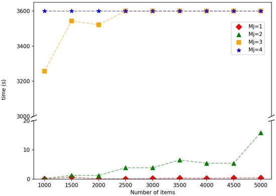
The computational complexity of multi-cover-type problems typically increases with the coverage thresholds. To isolate and explicitly examine this effect, we conduct additional experiments in which the activation thresholds are no longer generated randomly. Instead, all items are assigned a common threshold value $M_j$. The remaining parameters are fixed as $\left|I\right|=80$, $B=50$, and all instances are solved using the OA method. Figure 2 reports the solution times under varying numbers of items and different common threshold values. Each point in the figure represents the average solution time over ten randomly generated instances. As expected, the computational effort increases with the number of items. More importantly, a substantial escalation in solution time is observed as the common threshold $M_j$ increases. When $M_j=1$ or 2, all instances are solved within 20 s. For $M_j=3$, the solution time increases significantly, requiring more than 3000 s. When $M_j=4$, none of the instances can be solved to optimality within the prescribed time limit. These findings indicate that the activation threshold is a key factor influencing the intrinsic computational difficulty of the problem.

Figure 2. Solution times for different numbers of items and threshold values $M_j$.

6. Conclusions

This paper studies a class of optimization problems that maximize the expected value of a concave, strictly increasing utility function with explicit incorporation of activation thresholds, thereby addressing the growing demand for reliability in real-world applications. We formulate generalized models for this problem class, which lead to MINLP. To address the resulting nonlinearity, we employ SC and OA techniques to linearize the utility function, thereby reformulating the original model into two MILPs solvable by off-the-shelf solvers. Motivated by the superior performance of the OA method, we further develop a BD method that projects out item-related variables and dynamically generates the associated large-scale coupling constraints. This decomposition strategy significantly enhances the scalability of the proposed model and enables the efficient solution of ultra-large-scale instances. The numerical results indicate that the OA and BD methods possess complementary advantages across different problem scales. In particular, the OA method performs more efficiently for instances with the number of items in $\{\mathrm{20,000},\mathrm{30,000},\mathrm{40,000}\}$, whereas the BD method shows superior performance on larger instances with $\{\mathrm{100,000},\mathrm{150,000},\mathrm{200,000}\}$ items. By contrast, the SC method consistently yields inferior computational performance compared with the other two methods.

This study also suggests several promising directions for future research. From an application-oriented perspective, the proposed modeling framework and solution methods can be leveraged to enhance robustness in a variety of practical settings, including autonomous driving, social network analysis, and emergency response planning. The numerical findings further provide practical guidance for algorithm selection: the OA formulation is generally preferable for moderate-scale instances, whereas the BD approach offers superior scalability for ultra-large problems, enabling practitioners to select solution strategies according to dataset size and operational requirements. From a methodological standpoint, future work may focus on designing more advanced preprocessing techniques to reduce problem size and accelerate solution times. Although the SC method exhibits relatively weak performance in its current form, its effectiveness may be improved by strengthening the associated inequalities through lifting strategies. For structurally related problems without activation thresholds, several preprocessing techniques [47] as well as strengthened submodular cut formulations [1] have been studied in the literature. Extending these ideas to the more general setting considered in this paper remains a worthwhile direction for future research. Furthermore, developing parallel implementations of the proposed algorithms represents another important direction, with the potential to significantly improve scalability and facilitate the efficient solution of large-scale problems involving a greater number of scenarios.

References

- Ahmed, S.; Atamtürk, A. Maximizing a class of submodular utility functions. Math. Program. 2011, 128, 149–169. [Google Scholar] [CrossRef]
- Yu, J.; Ahmed, S. Maximizing a class of submodular utility functions with constraints. Math. Program. 2017, 162, 145–164. [Google Scholar] [CrossRef]
- Yu, J.; Ahmed, S. Maximizing expected utility over a knapsack constraint. Oper. Res. Lett. 2016, 44, 180–185. [Google Scholar] [CrossRef]
- Corner, J.L.; Corner, P.D. Characteristics of decisions in decision analysis practice. J. Oper. Res. Soc. 1995, 46, 304–314. [Google Scholar] [CrossRef]
- Aboolian, R.; Berman, O.; Krass, D. Competitive facility location model with concave demand. Eur. J. Oper. Res. 2007, 181, 598–619. [Google Scholar] [CrossRef]
- Feige, U. On maximizing welfare when utility functions are subadditive. In Proceedings of the 38th Annual ACM Symposium on Theory of Computing, Seattle, WA, USA, 21–23 May 2006; pp. 41–50. [Google Scholar]
- Coniglio, S.; Furini, F.; Ljubić, I. Submodular maximization of concave utility functions composed with a set-union operator with applications to maximal covering location problems. Math. Program. 2022, 196, 9–56. [Google Scholar] [CrossRef]
- Kempe, D.; Kleinberg, J.; Tardos, É. Maximizing the spread of influence through a social network. In Proceedings of the 9th ACM SIGKDD International Conference on Knowledge Discovery and Data Mining, Washington, DC, USA, 24–27 August 2003; pp. 137–146. [Google Scholar]
- Lehmann, B.; Lehmann, D.; Nisan, N. Combinatorial auctions with decreasing marginal utilities. In Proceedings of the 3rd ACM Conference on Electronic Commerce, Tampa, FL, USA, 14–17 October 2001; pp. 18–28. [Google Scholar]
- Ljubić, I.; Moreno, E. Outer approximation and submodular cuts for maximum capture facility location problems with random utilities. Eur. J. Oper. Res. 2018, 266, 46–56. [Google Scholar] [CrossRef]
- ReVelle, C.; Hogan, K. The maximum availability location problem. Transp. Sci. 1989, 23, 192–200. [Google Scholar] [CrossRef]
- Li, G.; Li, Y.; Zhang, W.; Chen, S. Benders decomposition approach for generalized maximal covering and partial set covering location problems. Symmetry 2025, 17, 1417. [Google Scholar] [CrossRef]
- Shi, Y.; Ran, Y.; Zhang, Z.; Willson, J.; Tong, G.; Du, D.Z. Approximation algorithm for the partial set multi-cover problem. J. Glob. Optim. 2019, 75, 1133–1146. [Google Scholar] [CrossRef]
- Ran, Y.; Shi, Y.; Tang, C.; Zhang, Z. A primal-dual algorithm for the minimum partial set multi-cover problem. J. Comb. Optim. 2020, 39, 725–746. [Google Scholar] [CrossRef]
- Revelle, C.; Hogan, K. The maximum reliability location problem and α-reliable p-center problem: Derivatives of the probabilistic location set covering problem. Ann. Oper. Res. 1989, 18, 155–173. [Google Scholar]
- ReVelle, C.; Hogan, K. A reliability-constrained siting model with local estimates of busy fractions. Environ. Plan. B Plan. Des. 1988, 15, 143–152. [Google Scholar] [CrossRef]
- Marianov, V.; ReVelle, C. The queueing maximal availability location problem: A model for the siting of emergency vehicles. Eur. J. Oper. Res. 1996, 93, 110–120. [Google Scholar] [CrossRef]
- Wang, W.; Wu, S.; Wang, S.; Zhen, L.; Qu, X. Emergency facility location problems in logistics: Status and perspectives. Transp. Res. Part E Logist. Transp. Rev. 2021, 154, 102465. [Google Scholar] [CrossRef]
- Berman, O.; Drezner, Z.; Krass, D. Discrete cooperative covering problems. J. Oper. Res. Soc. 2011, 62, 2002–2012. [Google Scholar] [CrossRef]
- Curtin, K.M.; Hayslett-McCall, K.; Qiu, F. Determining optimal police patrol areas with maximal covering and backup covering location models. Netw. Spat. Econ. 2010, 10, 125–145. [Google Scholar] [CrossRef]
- Reichlin, C.R.A. Non-Concave Utility Maximization:: Optimal Investment, Stability and Applications. Ph.D. Thesis, ETH Zurich, Zürich, Switzerland, 2012. [Google Scholar]
- Rahmattalabi, A.; Jabbari, S.; Lakkaraju, H.; Vayanos, P.; Izenberg, M.; Brown, R.; Rice, E.; Tambe, M. Fair influence maximization: A welfare optimization approach. In Proceedings of the AAAI Conference on Artificial Intelligence, Virtual, 2–9 February 2021; Volume 35, pp. 11630–11638. [Google Scholar]
- Wang, Z.; Zhao, J.; Sun, C.; Rui, X.; Yu, P.S. A general concave fairness framework for influence maximization based on poverty reward. ACM Trans. Knowl. Discov. Data 2024, 19, 1–23. [Google Scholar] [CrossRef]
- Shan, X.; Chen, W.; Li, Q.; Sun, X.; Zhang, J. Cumulative activation in social networks. Sci. China Inf. Sci. 2019, 62, 52103. [Google Scholar] [CrossRef]
- Romero, D.M.; Meeder, B.; Kleinberg, J. Differences in the mechanics of information diffusion across topics: Idioms, political hashtags, and complex contagion on twitter. In Proceedings of the 20th International Conference on World Wide Web, Hyderabad, India, 28 March–1 April 2011; pp. 695–704. [Google Scholar]
- Church, R.L.; Gerrard, R.A. The multi-level location set covering model. Geogr. Anal. 2003, 35, 277–289. [Google Scholar] [CrossRef]
- Snyder, L.V.; Daskin, M.S. Reliability models for facility location: The expected failure cost case. Transp. Sci. 2005, 39, 400–416. [Google Scholar] [CrossRef]
- Hauser, J.R.; Wernerfelt, B. An evaluation cost model of consideration sets. J. Consum. Res. 1990, 16, 393–408. [Google Scholar] [CrossRef]
- Messinger, P.R.; Narasimhan, C. A model of retail formats based on consumers’ economizing on shopping time. Mark. Sci. 1997, 16, 1–23. [Google Scholar] [CrossRef]
- Naples, M.J. Effective frequency: Then and now. J. Advert. Res. 1997, 37, 7–12. [Google Scholar] [CrossRef]
- Ostrow, J.W. Setting effective frequency levels. In Proceedings of the Effective Frequency: The State of the Art; Advertising Research Foundation, Key Issues Workshop: New York, NY, USA, 1982; pp. 89–102. [Google Scholar]
- Makienko, I. Effective frequency estimates in local media planning practice. J. Target. Meas. Anal. Mark. 2012, 20, 57–65. [Google Scholar] [CrossRef]
- Nemhauser, G.L.; Wolsey, L.A.; Fisher, M.L. An analysis of approximations for maximizing submodular set functions—I. Math. Program. 1978, 14, 265–294. [Google Scholar] [CrossRef]
- Wolsey, L.A.; Nemhauser, G.L. Integer and Combinatorial Optimization; John Wiley & Sons: Hoboken, NJ, USA, 1999. [Google Scholar]
- Shi, X.; Prokopyev, O.A.; Zeng, B. Sequence independent lifting for a set of submodular maximization problems. Math. Program. 2022, 196, 69–114. [Google Scholar] [CrossRef]
- Lamontagne, S.; Carvalho, M.; Atallah, R. Accelerated Benders decomposition and local branching for dynamic maximum covering location problems. Comput. Oper. Res. 2024, 167, 106673. [Google Scholar] [CrossRef]
- Nemhauser, G.; Wolsey, L. Matroid and Submodular Function Optimization. In Integer and Combinatorial Optimization; John Wiley & Sons, Ltd.: Hoboken, NJ, USA, 1988; Chapter 3; pp. 659–719. [Google Scholar]
- Padberg, M.; Rinaldi, G. A branch-and-cut algorithm for the resolution of large-scale symmetric traveling salesman problems. SIAM Rev. 1991, 33, 60–100. [Google Scholar] [CrossRef]
- Wolsey, L.A. Integer Programming; John Wiley & Sons: Hoboken, NJ, USA, 2020. [Google Scholar]
- Fischetti, M.; Ljubić, I.; Sinnl, M. Benders decomposition without separability: A computational study for capacitated facility location problems. Eur. J. Oper. Res. 2016, 253, 557–569. [Google Scholar] [CrossRef]
- Cordeau, J.F.; Furini, F.; Ljubić, I. Benders decomposition for very large scale partial set covering and maximal covering location problems. Eur. J. Oper. Res. 2019, 275, 882–896. [Google Scholar] [CrossRef]
- Güney, E.; Leitner, M.; Ruthmair, M.; Sinnl, M. Large-scale influence maximization via maximal covering location. Eur. J. Oper. Res. 2021, 289, 144–164. [Google Scholar] [CrossRef]
- Di Summa, M.; Grosso, A.; Locatelli, M. Branch and cut algorithms for detecting critical nodes in undirected graphs. Comput. Optim. Appl. 2012, 53, 649–680. [Google Scholar] [CrossRef]
- Pavlikov, K. Improved formulations for minimum connectivity network interdiction problems. Comput. Oper. Res. 2018, 97, 48–57. [Google Scholar] [CrossRef]
- CPLEX. User’s Manual for CPLEX; IBM: Armonk, NY, USA, 2022; Available online: https://www.ibm.com/docs/en/icos/20.1.0?topic=cplex-users-manual (accessed on 16 January 2026).
- ReVelle, C.; Scholssberg, M.; Williams, J. Solving the maximal covering location problem with heuristic concentration. Comput. Oper. Res. 2008, 35, 427–435. [Google Scholar] [CrossRef]
- Chen, S.J.; Chen, W.K.; Dai, Y.H.; Yuan, J.H.; Zhang, H.S. Efficient presolving methods for the influence maximization problem. Networks 2023, 82, 229–253. [Google Scholar] [CrossRef]
Disclaimer/Publisher’s Note: The statements, opinions and data contained in all publications are solely those of the individual author(s) and contributor(s) and not of MDPI and/or the editor(s). MDPI and/or the editor(s) disclaim responsibility for any injury to people or property resulting from any ideas, methods, instructions or products referred to in the content. |
© 2026 by the authors. Licensee MDPI, Basel, Switzerland. This article is an open access article distributed under the terms and conditions of the Creative Commons Attribution (CC BY) license.