


Abstract
Wind represents a pervasive yet mechanistically distinct environmental factor that reshapes species interactions primarily through habitat compression—reducing effective habitat area via behavioral avoidance, rather than altering resource availability as seen in temperatureor rainfall-driven models. This study introduces a a novel wind-modified Lotka–Volterra competition model that advances existing disturbance-dependent frameworks through two key innovations: (1) a wind-speed-dependent carrying capacity, formally expressed as the initial carrying capacity divided by a linear function of wind speed and species-specific wind sensitivity, which explicitly quantifies wind-induced habitat contraction as a nonlinear function of wind exposure; and (2) a species-specific wind sensitivity coefficient that can be experimentally calibrated. Through a rigorous stability analysis and numerical simulations, we demonstrate how wind speed modulates competitive outcomes by altering equilibrium densities and stability. Our results reveal: (a) wind can reverse competitive dominance, disproportionately excluding species with higher wind sensitivity coefficients; (b) critical wind speed thresholds exist, beyond which populations collapse due to mechanisms akin to Allee effects and demographic stochasticity; and (c) wind nonlinearly regulates coexistence, with moderate speeds sometimes stabilizing it and extreme speeds driving effective extinction. This framework provides a theoretical foundation for setting conservation thresholds and assessing the ecological impacts of wind energy projects.
Keywords:
wind-modified Lotka–Volterra model; carrying capacity shrinkage; wind sensitivity coefficient; competitive exclusion threshold; ecological impact assessment MSC:
34A34; 37B55; 34D05; 37N25
1. Introduction
Interspecific competition is a fundamental ecological process that governs population dynamics, community assembly, and biodiversity. Classical competition theory, anchored in the Lotka–Volterra model, has provided profound insights into how species coexist or exclude one another under stable environmental conditions [1,2,3,4,5,6]. Extensions of this framework have incorporated various biological and environmental complexities—such as Allee effects [7,8,9], toxic substances [10,11], stage structure [12], fear effects [13], impulsive disturbances [14], time delays [15,16], stochastic disturbances [16,17,18,19], feedback control [11,15], and disease [20]—enhancing our understanding of the mechanisms driving competitive outcomes.
Research on stage-structured populations [12,17] has revealed how competition at different life stages influences population dynamics. Pulse effects [14] focus on the impact of sudden changes in environmental or biological processes on competitive systems. Fear-induced behavioral changes examine how the presence of competitor species affects the behavior and distribution of the other populations [13]. Feedback control mechanisms explore how internal or inter-population feedback regulates competitive processes [11,15]. Delay-induced dynamics analyze how time delays influence the stability and behavior of competitive systems [15,16].
Additionally, studies on Allee effects [7,8,9] demonstrate that when population density falls below a critical threshold, reproductive and survival rates decline significantly, which in turn affects competitive outcomes. These research efforts have significantly advanced our understanding of how species compete for limited resources and how these interactions influence population stability and coexistence.
However, a critical gap remains in the systematic modeling of interspecific competition under dynamic environmental conditions, particularly those influenced by atmospheric disturbances such as wind. Wind, as a pervasive environmental factor, exerts profound, yet often overlooked, impacts on species interactions. Ecological studies have documented that strong winds can alter animal behavior, including avian migration patterns [21] and insect flight capacities [22], as well as habitat structure through vegetation sway [23]. These changes effectively reduce the available habitat area for species, thereby influencing their population dynamics.
Despite these findings, existing research predominantly focuses on individual-level physiological or behavioral responses to wind [24,25,26,27] or predator–prey interactions [28,29,30,31,32,33,34,35]. The population-level competitive dynamics under varying wind conditions remain inadequately modeled. This gap hinders our ability to address key ecological questions:
- Mechanistic level: How does wind-induced habitat contraction reshape interspecific competitive balances, and what are the thresholds beyond which species experience competitive exclusion?
- Applied level: Under the projected global increase in wind speeds [25], how can we predict and mitigate extinction risks for wind-sensitive species, particularly in the context of renewable energy development?
To address these questions, we propose a novel modification to the classical Lotka–Volterra competition model by incorporating wind-speed-dependent carrying capacity and wind sensitivity coefficients. This approach enables the quantification of habitat loss due to wind and allows for the calibration of species-specific responses to varying wind intensities. Our model provides a theoretical framework to analyze how wind-driven habitat changes influence competitive outcomes, offering insights for biodiversity conservation and ecological management.
The remainder of this paper is structured as follows: Section 2 presents the mathematical formulation of the modified Lotka–Volterra model, including the derivation of wind-speed-dependent carrying capacities. Section 3 and Section 4 investigate the existence and local stability of equilibrium points under varying wind conditions, respectively. Section 5 and Section 6 investigate the global stability of the positive equilibrium and boundary equilibrium, respectively. Numerical simulations in Section 7 illustrate the model’s predictions, Section 8 discusses the ecological implications of our findings, and Section 9 presents their practical applications.
2. Model Construction
The classical Lotka–Volterra competition model is described as
Based on ecological observations, strong winds cause animals to avoid high-wind zones (e.g., reduced avian activity in open areas [24]), leading to decreased effective habitat area. This habitat reduction can be quantified as
The modified competition model with wind-speed-dependent carrying capacity becomes
For the ecological interpretation of parameters, see Table 1.
Table 1.
Model parameters and their ecological interpretations.
The fundamental theoretical innovation of our model resides in the replacement of static carrying capacities () with wind-velocity dependent functions, defined as . This mathematical formulation captures three essential ecological phenomena: effective habitat area diminishes nonlinearly with increasing wind velocity, species demonstrate differential sensitivity to wind exposure (), and competitive stability transitions from static to environmentally contingent.
This investigation addresses three interconnected questions regarding wind-mediated competition dynamics. First, we examine how wind velocity modulates equilibrium population densities in competing species systems. Second, we evaluate whether heightened wind exposure induces competitive exclusion in wind-sensitive taxa. Third, we identify critical wind velocity thresholds that precipitate local species extinction, thereby establishing environmental boundaries for coexistence.
This model facilitates understanding of wind-driven community dynamics and enables assessment of climate change impacts (e.g., increased extreme wind events [25]) on biodiversity. Additionally, the results inform ecological evaluations of wind energy installations (e.g., wind farm siting impacts on wildlife [26]).
3. Existence of Equilibrium Points
The trivial equilibrium exists for all parameter values.
For , we solve
Thus, always exists.
For , we solve
Thus, always exists.
The positive equilibrium satisfies
The solution is
Existence conditions:
- Case 1:which can be rewritten as
- Case 2:which can be rewritten as
Theorem 1.
Remark 1.
The wind-modified carrying capacity exhibits the fundamental property
The system admits formal equilibrium solutions , where are defined by (5). Despite mathematical existence, extreme winds induce
creating an effective extinction scenario. The extinction mechanisms are stated in Table 2.
Table 2.
Small-population vulnerabilities.
4. Local Stability of Equilibrium Points
Regarding the local stability of equilibrium points in system (3), we have the following results:
Theorem 2.
is always unstable; is stable when , otherwise unstable; is stable when , otherwise unstable; When and (corresponding to Case 1 of positive equilibrium existence), the positive equilibrium is stable. Under Case 2 of positive equilibrium existence, the positive equilibrium is unstable.
Proof.
See Appendix A. □
Remark 2.
Wind effect analysis:
Given , wind impacts manifest as follows:
- When , decreases faster, potentially causing and stabilizing (species 1 exclusion);
- When , decreases faster, potentially causing and stabilizing (species 2 exclusion);
- Extreme wind () drives system toward (dual extinction). However, is unstable, indicating that under extreme wind speeds, although the population may not eventually converge to zero, the value it converges to is still sufficiently close to zero—meaning the population size becomes extremely small.
Remark 3.
Wind disturbance generates striking ecological stability shifts, revealing several non-trivial dynamics that qualitatively depart from the predictions of the classical Lotka–Volterra model with fixed parameters. First, wind can reverse competitive dominance when species’ asymmetry parameters () diverge, causing subordinate species to outperform dominants (competitive reversal; Figure A5). This demonstrates that competitive outcomes are not static but environmentally plastic. Second, critical extinction thresholds () exist, where exceeding wind speeds triggers abrupt species collapse; a threshold-driven dynamic inherent to the nonlinear decay of . Most paradoxically, under extreme winds (), population equilibria () approach zero (while remaining positive) despite instability in the windless equilibrium ()—revealing a distinct effective extinction state where species persist theoretically but decline to ecologically nonfunctional densities. Most significantly, the model predicts coexistence windows at moderate wind velocities , where stable coexistence emerges solely due to wind-mediated habitat compression—an outcome impossible under static carrying capacities. Thus, while mathematically akin to parameter substitution, the wind-dependent formulation fundamentally transforms the model from predicting fixed outcomes to capturing environmentally contingent community assembly.
5. Global Stability of the Coexistence Equilibrium
A central question in species coexistence theory is whether competitive outcomes remain robust under environmental variability. Here, we investigate how wind-driven habitat compression affects the global stability of competitive systems—that is, whether populations inevitably converge to equilibrium regardless of initial densities.
Theorem 3.
Assume that
holds. Then, system (3) admits a unique positive equilibrium point that is globally asymptotically stable.
Proof.
Using Lyapunov stability theory, we confirm global convergence to when (12) is satisfied. The mathematical approach follows standard techniques for Lotka–Volterra systems but incorporates the critical innovation of wind-dependent parameters. The full derivation is provided in Appendix B. □
Remark 4.
For the coexistence equilibrium to be globally asymptotically stable (i.e., attracting all trajectories with positive initial densities), two conditions in (12) must simultaneously hold. These inequalities represent ecological balance requirements:
- Species 1’s habitat capacity must exceed competitive pressure from Species 2;
- Species 2’s habitat capacity must exceed competitive pressure from Species 1.
Remark 5.
Theorem 3 reveals three distinct mechanisms by which wind regimes reconfigure competitive stability. First, competitive reversal occurs when dominant species under calm conditions () face exclusion under elevated wind speeds () due to their heightened wind sensitivity (), where accelerated habitat loss violates fundamental stability conditions. Second, emergent coexistence windows arise at moderate wind velocities (), stabilizing species coexistence that remains unattainable in windless scenarios, as demonstrated in Figure A5. Third, threshold-driven extinction cascades manifest at critical wind speeds , characterized by abrupt population collapse, where while , disproportionately impacting wind-sensitive taxa through discontinuous phase transitions in community structure.
Conventional Lotka–Volterra models predict invariant competitive outcomes based solely on static competition coefficients () and carrying capacities, whereas our framework reveals three fundamental departures. First, competitive hierarchies exhibit significant environmental plasticity, with wind-tolerant species gaining advantages independent of their baseline competitive ability. Second, community stability proves environmentally contingent, as identical species pairs may transition between coexistence and exclusion regimes depending on wind conditions. Third, we identify a critical sensitivity threshold, s/m, that predicts elevated extinction risk across taxonomic groups, indicating universal biomechanical constraints on persistence.
The wind-dependent stability conditions elucidated by our model resolve longstanding discrepancies in field observations, particularly, abrupt community shifts in exposed ecosystems that remain irreproducible by static carrying capacity models. These findings directly inform conservation strategies: wind exposure zones should be demarcated using species-specific critical wind thresholds (), protection priorities must be reassigned to high-sensitivity () species regardless of current dominance status, and wind farm buffer designs require -weighted vulnerability assessments to mitigate cascading ecological impacts.
Remark 6
(Validity under high wind). The global stability proof of (Theorem 3) requires and . These conditions are naturally satisfied within the wind regime where exists (i.e., where inequalities (12) hold). Crucially, as wind speed increases, the existence conditions (12) are violated before the mathematical premises of the Lyapunov proof break down. This means the theorem correctly describes the system’s behavior precisely when coexistence is possible. In the high-wind regime, where , the coexistence equilibrium no longer exists, and stability is determined by the boundary equilibria (Theorems 2 and 5). Thus, the Lyapunov analysis remains rigorous throughout the ecologically relevant parameter domain.
6. Global Stability Analysis of Boundary Equilibrium Points
Before presenting global stability results for boundary equilibria, we first address the limit cycle existence problem for system (3).
Theorem 4.
System (3) contains no limit cycles.
Proof.
Select the Dulac function as
Calculate the divergence of the weighted vector field:
noting that
Thus,
In the positive quadrant:
- ;
- The parameters satisfy: .
Therefore,
By Dulac’s criterion, system (3) contains no limit cycles in the positive quadrant. □
Remark 7.
The proof of Theorem 4 holds for the case of finite wind speed (w). Due to the ecological implications of system (3), the wind speed cannot be infinite. Hence, Theorem 4 does not consider the case that wind speed (w) approaches infinity.
Theorem 5.
- 1.
- When and , is globally stable.
- 2.
- When and , is globally stable.
Proof.
- When and , Theorem 2 implies is locally stable. The trivial equilibrium is unstable, is unstable, and no positive equilibrium exists. Theorem 4 confirms that the system’s limit sets can only be equilibrium points, therefore is globally stable.
- When and , Theorem 2 implies is locally stable. The trivial equilibrium is unstable, is unstable, and no positive equilibrium exists. Theorem 4 again confirms the system’s limit sets must be equilibrium points, therefore is globally stable.
□
7. Numerical Simulations
Example 1.
In (3), set . Calculations show that
Without considering wind effects, the classical Lotka–Volterra competition system predicts that is globally asymptotically stable, as shown in Figure A1.
Now, we consider wind effects.
- (1)
- Set representing wind sensitivity coefficients, with the first population being more sensitive to wind.
- (a)
- For , calculations show thatBy Theorem 3, the unique positive equilibrium is globally asymptotically stable, as shown in Figure A2.
- (b)
- For , calculations show thatBy Theorem 5, the boundary equilibrium is globally asymptotically stable, as shown in Figure A3.
- (c)
- For , calculations show thatBy Theorem 5, the boundary equilibrium is globally asymptotically stable, as shown in Figure A4.These simulations illustrate that without wind, the first population dominates and excludes the second. However, as wind increases:
- The first population (more wind-sensitive) loses its competitive advantage;
- Moderate wind speeds () can stabilize coexistence;
- Higher winds () lead to competitive exclusion of the first population;
- Extreme winds () drive both populations toward extinction; at extremely high wind speeds, the second population (the wind-insensitive one) may persist but with low density.
To more clearly illustrate the impact of wind speed on the final equilibrium densities of the two populations, we plotted a bifurcation diagram (see Figure A5). From the diagram, it can be observed that there exist two critical wind speed values:- When the wind speed w is below the first critical value , the first population dominates while the second population goes extinct.
- When the wind speed w lies between the two critical values (), the two populations can coexist. However, as wind speed increases, the equilibrium density of the first population monotonically decreases, whereas that of the second population monotonically increases.
- When the wind speed exceeds the second critical value , the second population dominates, and the first population goes extinct.
That is to say, a population that is competitively dominant under windless conditions will eventually become competitively disadvantaged and tend toward extinction as wind speed increases, if it exhibits wind sensitivity.
- (2)
- Set making the second population more wind-sensitive.
- (a)
- For , calculations show thatBy Theorem 5, the boundary equilibrium is globally asymptotically stable, as shown in Figure A7.
- (b)
- For , calculations show thatBy Theorem 5, the boundary equilibrium is globally asymptotically stable, as shown in Figure A8.These results show that when the second population is more wind-sensitive, increasing wind:
- Maintains the first population’s dominance;
- Gradually reduces equilibrium densities of both populations;
- Does not lead to competitive reversal.
To better understand the impact of wind speed on the final equilibrium densities of both populations, we constructed a bifurcation diagram (see Figure A6). The diagram reveals that when the first population dominates while the second population remains wind-sensitive, the first population maintains its dominance across increasing wind speeds. However, its final equilibrium density shows a consistent monotonic decrease as wind speed continues to rise.
Link to extinction mechanisms.
The simulation results illustrate how wind stress can engage different extinction pathways. In Figure A3 (), the exclusion of the wind-sensitive species follows a trajectory where demographic stochasticity would amplify its decline once the population becomes small. In Figure A4 (), both populations are driven to extremely low densities (), entering a regime where Allee effects (due to mate-finding difficulty) and heightened vulnerability to environmental stochasticity would make deterministic persistence ecologically meaningless.
Example 2.
In (3), set
. Calculations show that
Without considering wind effects, the classical Lotka–Volterra competition system predicts that is globally asymptotically stable, as shown in Figure A9.
Now, we consider wind effects.
- (1)
- Set representing equal wind sensitivity coefficients for both populations. For , calculations show thatBy Theorem 3, the unique positive equilibrium is globally asymptotically stable, as shown in Figure A10.This example demonstrates that in a symmetric competition model, increasing wind speed:
- Maintains stable coexistence at a unique positive equilibrium;
- Progressively reduces the equilibrium population densities.
To elucidate the effects of wind speed on the final equilibrium densities of symmetrically competing populations with positive equilibrium points, we constructed a bifurcation diagram (see Figure A13). The analysis reveals that while both populations maintain stable coexistence with increasing wind speed, their equilibrium densities exhibit a gradual decline. - (2)
- Now, set making the first population more wind-sensitive.
- (a)
- For , calculations show thatBy Theorem 5, the boundary equilibrium is globally asymptotically stable, as shown in Figure A11.This case illustrates how in a system with stable coexistence:
- Increasing wind speed causes the wind-sensitive population to lose competitive advantage;
- Eventually leads to extinction of the sensitive species.
- (b)
- For , calculations show thatBy Theorem 5, the boundary equilibrium is globally asymptotically stable, as shown in Figure A12.Comparing cases (a) and (b) reveals the following:
- The less wind-sensitive population maintains dominance;
- Its equilibrium density still decreases with increasing wind speed;
- The system remains unstable under wind effects.
To clearly characterize the wind speed effects on population equilibrium densities, we performed a bifurcation analysis (see Figure A14). The system exhibits threshold dynamics governed by a critical wind speed .
- Subcritical regime ():
- –
- Stable coexistence persists;
- –
- Population 1 shows monotonic density decrease with increasing w;
- –
- Population 2 displays unimodal response:where represents the transition point.
- Supercritical regime ():
- –
- Competitive exclusion occurs;
- –
- Population 2 dominates ();
- –
- Population 1 goes extinct ().
These numerical simulations illustrate that for originally stable competitive systems:
- Wind reduces equilibrium population densities;
- Causes wind-sensitive populations to gradually lose competitive advantage;
- Ultimately leads to extinction of sensitive species;
- Wind introduces destabilizing effects on the system.
Example 3.
In system (3), set parameters as , , , . Calculations show that
Without wind effects (), the classical Lotka–Volterra competition system exhibits bistability—solutions converge to different boundary equilibria depending on initial values, as shown in Figure A15.
Now, consider wind effects:
- (1)
- Set , (equal wind sensitivity). For ,
By Theorem 2:
- Boundary equilibria and are locally asymptotically stable;
- Positive equilibrium is unstable.
Figure A16 confirms these results. This demonstrates that wind preserves bistability in symmetric systems while reducing equilibrium densities.
- (2)
- Set , (species 1 more wind-sensitive). For ,
By Theorem 2:
- Boundary equilibria and remain locally stable;
- Positive equilibrium remains unstable.
Figure A17 shows the expanded basin of attraction for the less sensitive species.
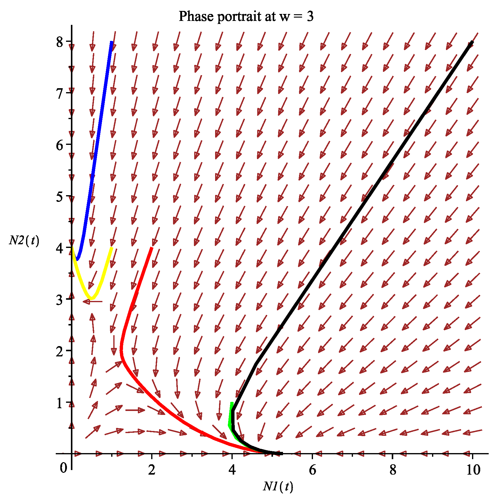
- (3)
- Set , (species 2 more wind-sensitive). For ,
By Theorem 2:
- Boundary equilibria and maintain stability;
- Positive equilibrium remains unstable.
Figure A18 demonstrates asymmetric stability regions under differential wind sensitivities.
Key observations:
- Wind preserves bistability but modifies attraction basins;
- Wind-sensitive species exhibit reduced stability regions;
- Equilibrium densities decrease with wind speed following ;
- Asymmetric sensitivities induce non-reciprocal competition outcomes.
8. Discussion
Our results fundamentally challenge the paradigm of static carrying capacities in competition ecology. By revealing wind’s capacity to invert competitive hierarchies through habitat compression rather than direct mortality, we identify three novel mechanisms: (1) Threshold-driven regime shifts, where 2 m/s wind doubles habitat compression rates for sensitive species; (2) emergent coexistence windows (2–5 m/s) through spatial niche separation; and (3) non-reciprocal exclusion, where traditional competitive dominants become climate losers under wind stress.
This habitat-mediated competition mechanism explains field observations of abrupt community shifts in wind-exposed ecosystems [12,13] that static-K models cannot replicate. Crucially, wind-tolerant “climate winner” species showed no correlation with traditional competitive ability (), suggesting new conservation metrics are needed.
Potential applications. Our framework suggests that wind-sensitivity coefficients () and critical wind speeds () could, in principle, inform conservation planning—for example, in identifying potentially vulnerable species during wind farm siting or in anticipating competitive shifts under changing wind regimes. However, these applications remain hypothetical and would require empirical calibration of and for real species. The qualitative match between our predicted thresholds (e.g., the 5 m/s mutual extinction threshold) and some observed collapse points in coastal insect communities [36] illustrates how the model could help interpret field patterns, not that it is a validated predictive tool.
9. Conclusions
This study advances competition theory through three key innovations: (1) dynamic carrying capacities capturing real-world habitat modifications, (2) measurable wind sensitivity coefficients () bridging microclimate ecology with population dynamics, and (3) quantifiable wind thresholds () predicting community transitions. Our model predicts fluid competitive hierarchies under wind stress, with dominance shifting to wind-tolerant species regardless of baseline competitive abilities. Crucially, extinction cascades emerge from asymmetric habitat reduction rather than direct mortality—a novel mechanism requiring conservation strategies to prioritize wind-sensitive competitors even when currently dominant.
The theoretical framework enables three practical applications: (1) designing wind buffers in protected areas using species-specific values, (2) optimizing wind farm placement through -based risk assessments, and (3) predicting climate change impacts via wind sensitivity rankings. Future extensions incorporating spatial wind heterogeneity and nonlinear responses could further enhance predictive accuracy for ecosystem management. By quantifying how atmospheric dynamics reshape terrestrial competition, this work establishes a critical interface between climate physics and community ecology.
Author Contributions
Writing—original draft preparation, Q.Y. and F.C.; writing—review and editing, Q.Y. and F.C. All authors have read and agreed to the published version of the manuscript.
Funding
This research was funded by the Anhui Provincial Research Center for Eco-agriculture of Chinese Medicinal Herbs Research Platform Project; 2024 school-level Scientific Research Project (Research on Population Characteristics of Wild Dendrobium huoshanense Based on Biodynamic Model); school-level Quality Engineering Project (wxxy2024115); Key Project of Humanities and Social Sciences Research, Department of Education of Anhui Province (2025AHGXSK30179) and the Natural Science Foundation of Fujian Province (2024J01273).
Data Availability Statement
No new data were created or analyzed in this study.
Conflicts of Interest
The authors declare no conflicts of interest.
Appendix A. Proof of Theorem 2
The Jacobian matrix of the system is
The partial derivatives are
At trivial equilibrium ,
Eigenvalues , , hence is always unstable.
At boundary equilibrium ,
Eigenvalues:
From the above equalities, one can see that if holds, consequently, is locally stable. Otherwise is unstable.
At boundary equilibrium ,
Eigenvalues:
From the above equalities, one can see that if holds, consequently, is locally stable. Otherwise is unstable.
At positive equilibrium ,
Characteristic equation:
When and , it immediately follows that (i.e., ) and , consequently, the two solutions of Equation (A6) have negative real parts, and the positive equilibrium is locally stable. Under Case 2, leads to positive real parts of eigenvalues, making the positive equilibrium unstable.
This ends the proof of Theorem 2.
Appendix B. Proof of Theorem 3
Proof.
Define the Lyapunov function:
where are constants to be determined. This function satisfies
- ;
- ;
- .
Differentiating along system trajectories:
Using equilibrium conditions and , we rewrite as
Let , , then
where
The quadratic form is a negative definite if matrix is positive definite, requiring the following:
- and (trivially satisfied);
- Determinant .
Choose coefficients , , yielding
The determinant becomes
When , the determinant is positive, making the matrix positive definite. Thus is negative definite, and by Lyapunov’s stability theorem, is globally asymptotically stable.
This ends the proof of Theorem 3. □
Figure A1.
Example 1 (): The boundary equilibrium is globally asymptotically stable.
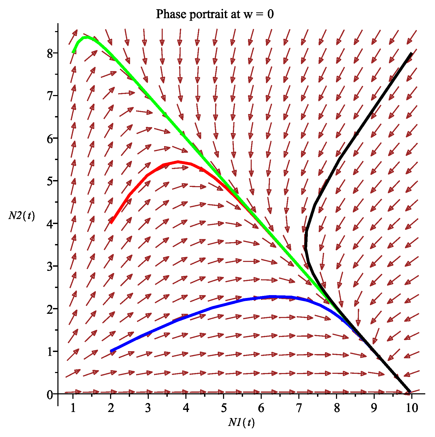
Figure A2.
Example 1 (): The positive equilibrium (1.71,4.44) is globally asymptotically stable.
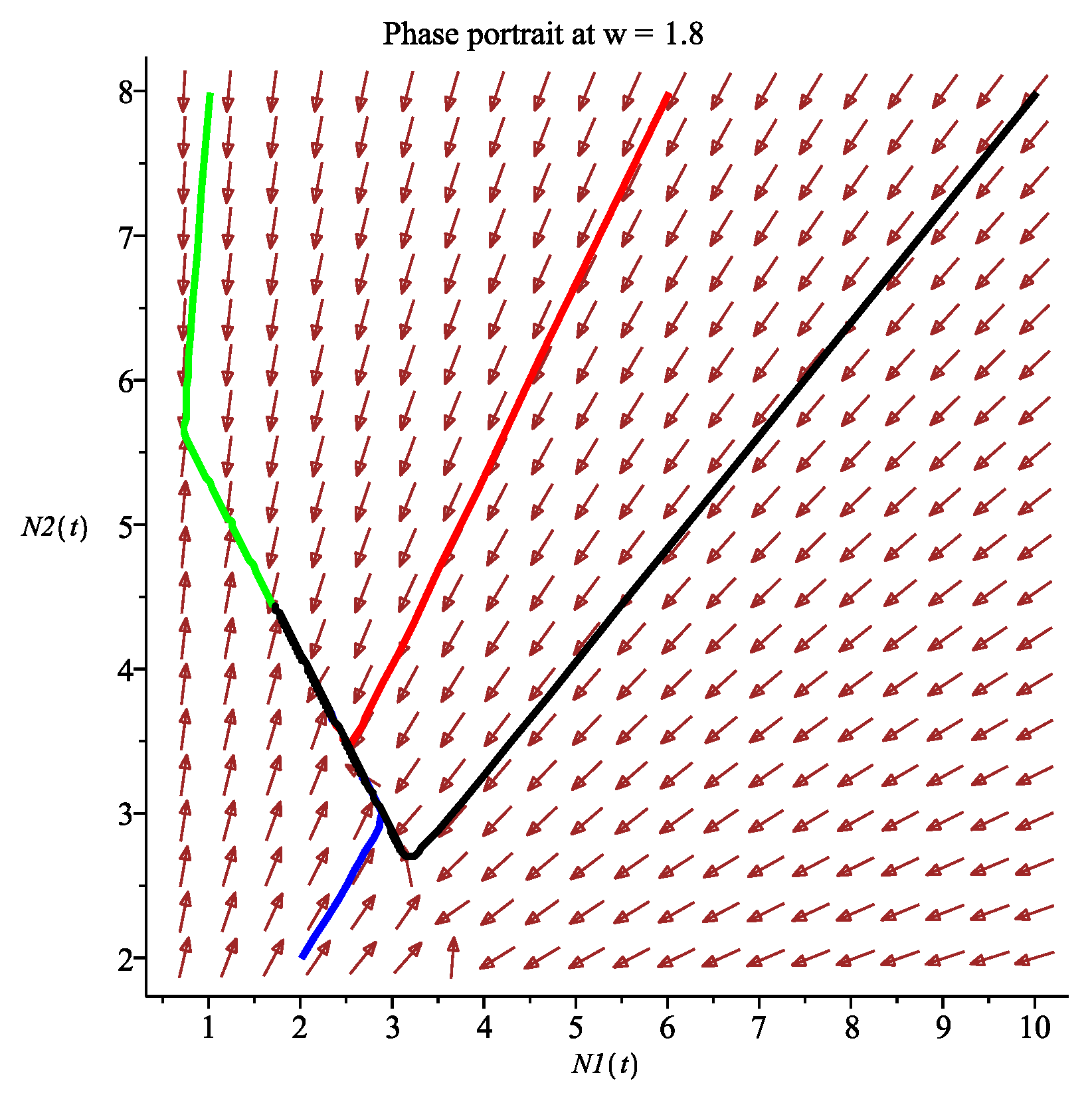
Figure A3.
Example 1 (): The boundary equilibrium is globally asymptotically stable.
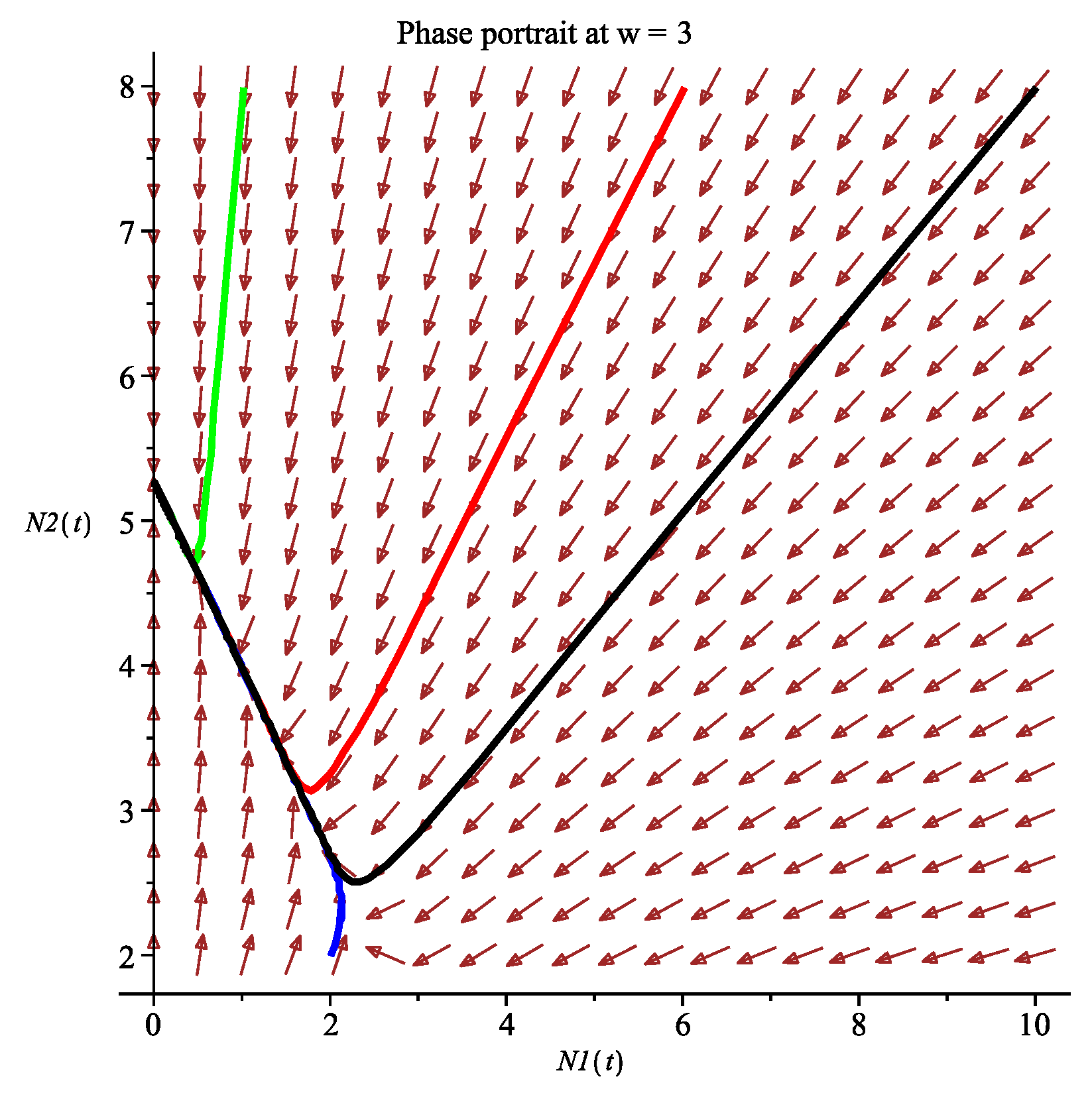
Figure A4.
Example 1 (): The boundary equilibrium is globally asymptotically stable.
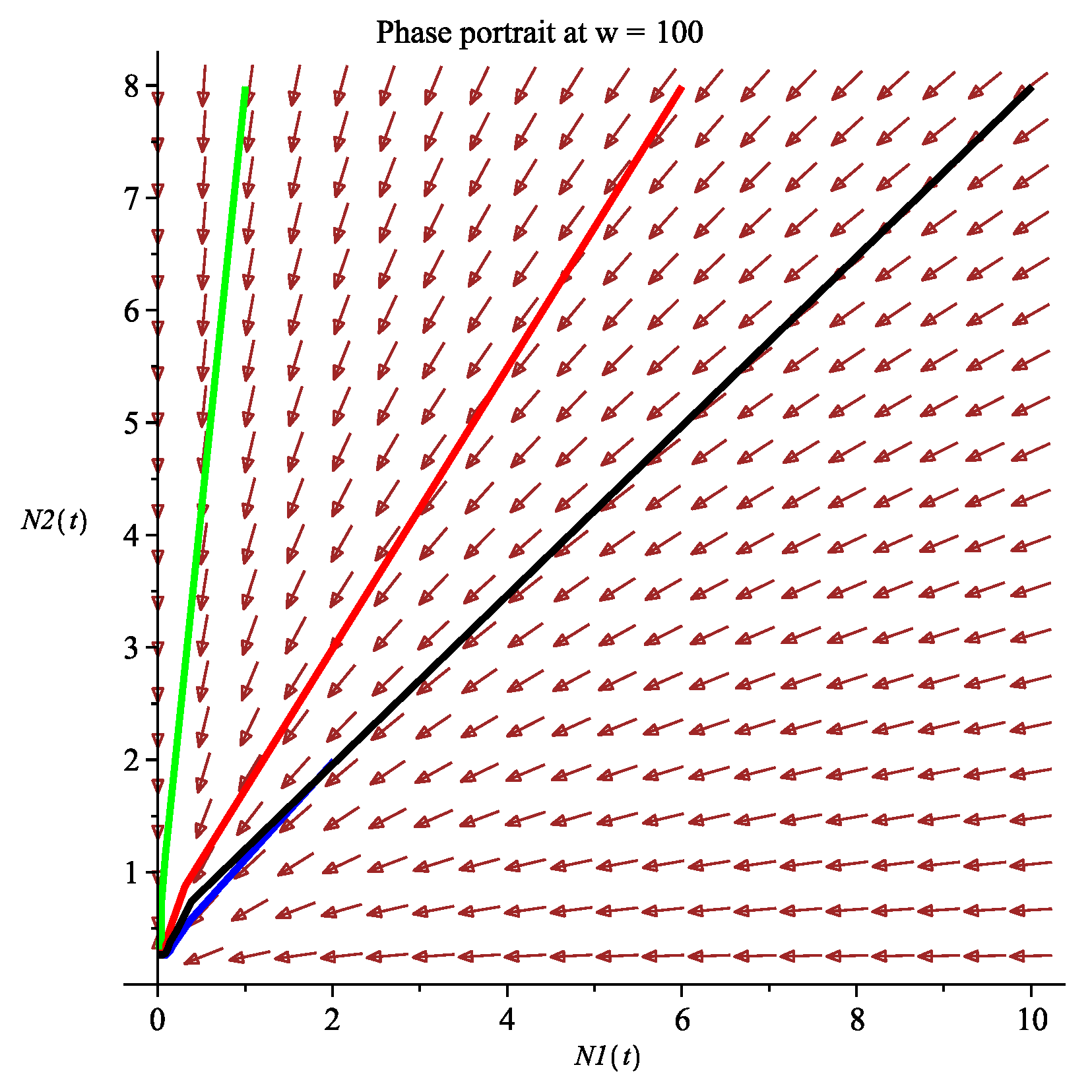
Figure A5.
Example 1, Case (1): Bifurcation diagram of the final equilibrium population densities versus wind speed.
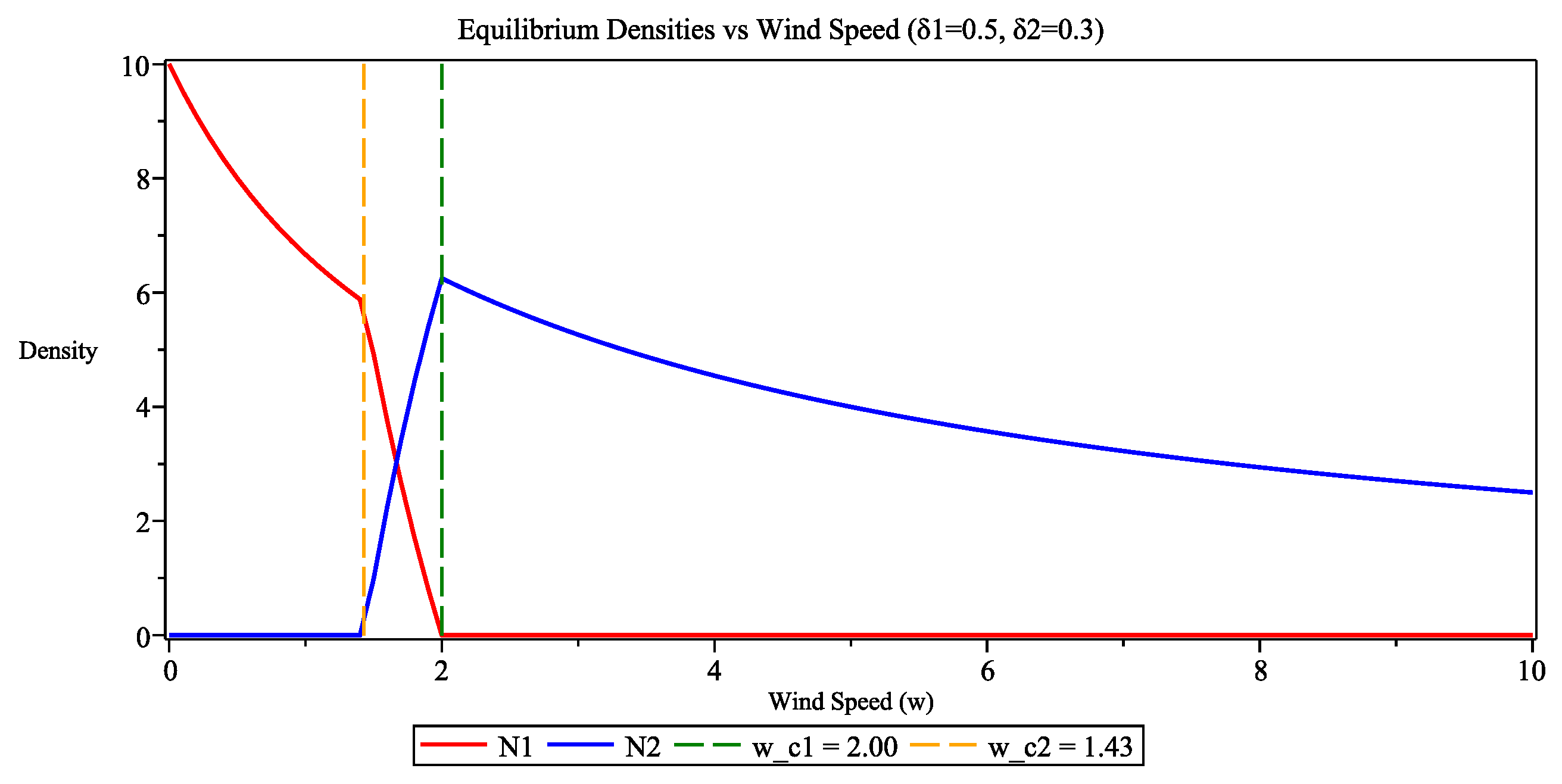
Figure A6.
Example 1, Case (2): Bifurcation diagram of the final equilibrium population densities versus wind speed.
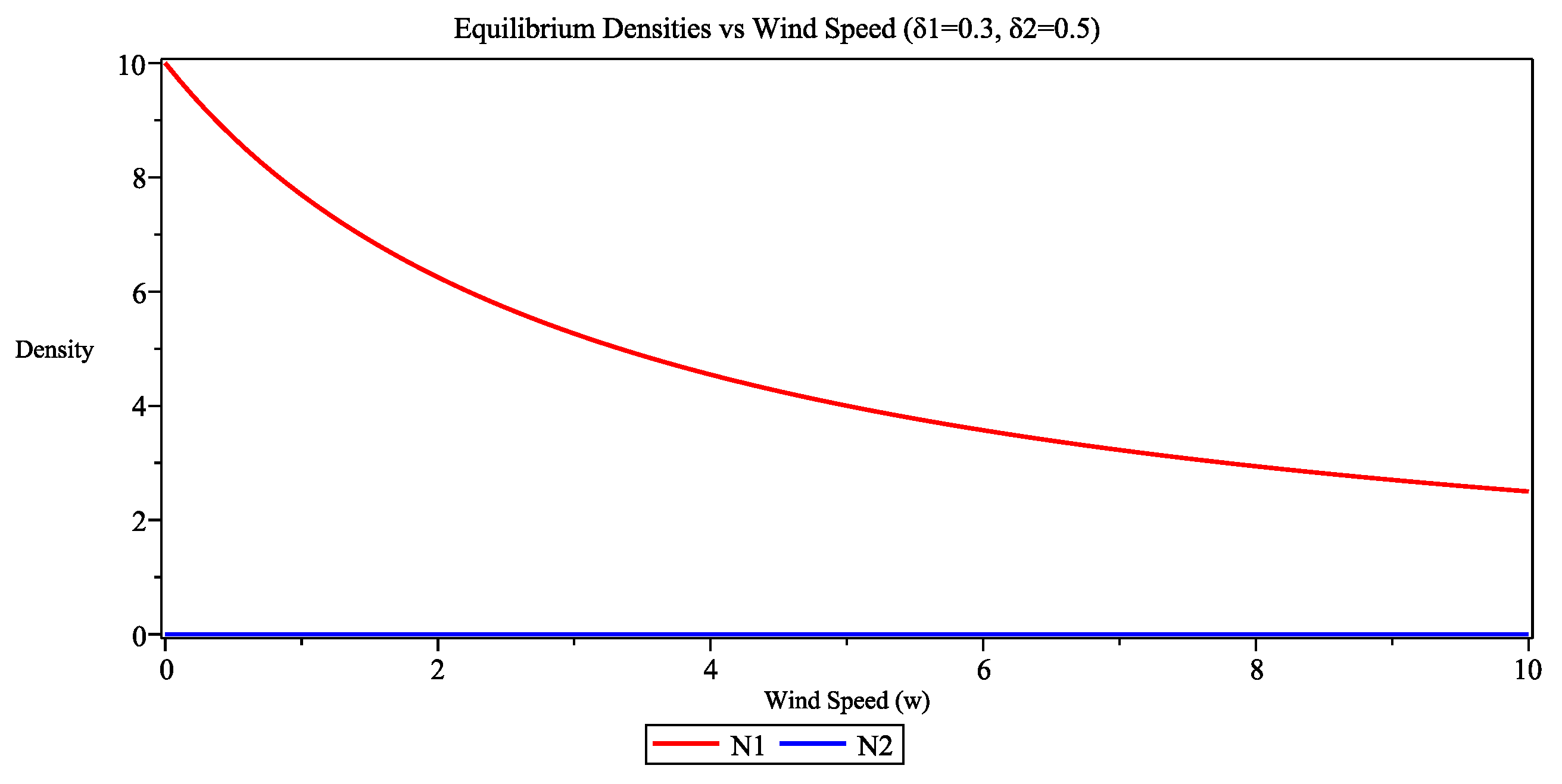
Figure A7.
Example 1 (): The boundary equilibrium is globally asymptotically stable.
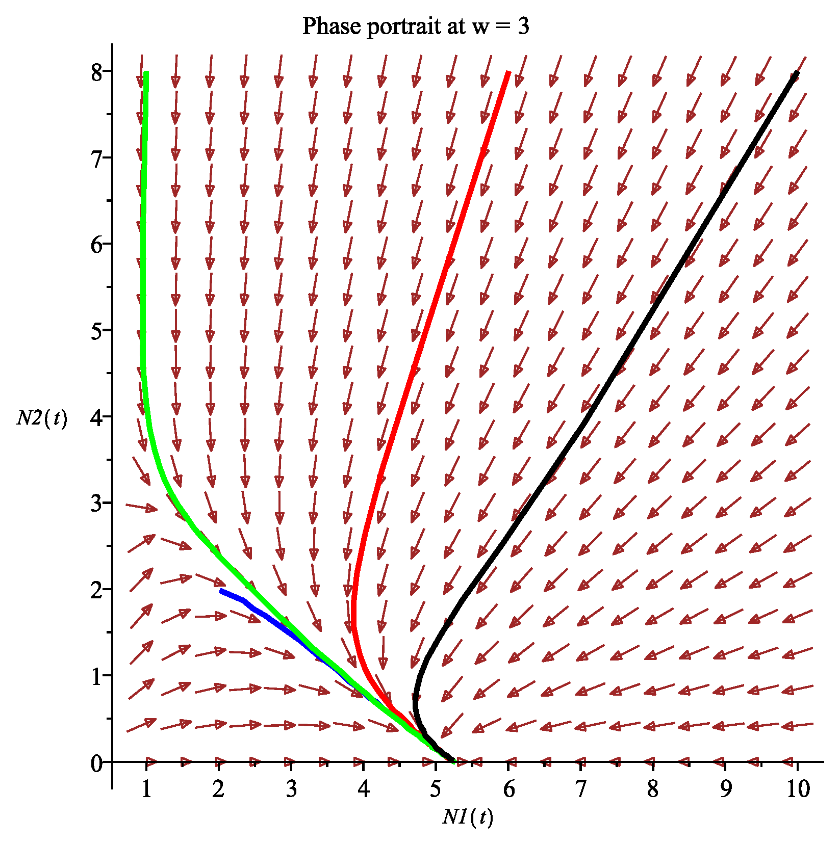
Figure A8.
Example 1 (): The boundary equilibrium is globally asymptotically stable.
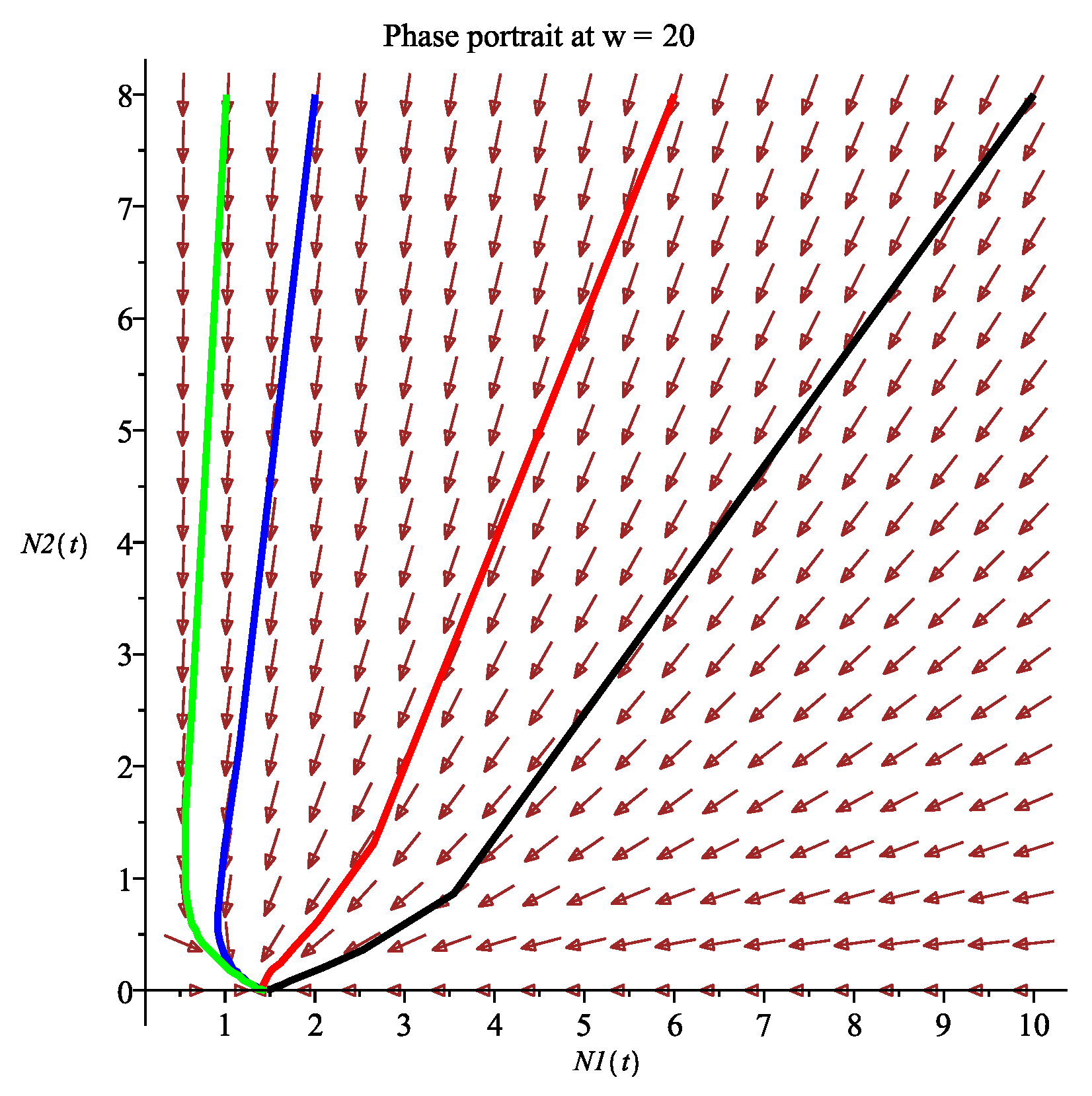
Figure A9.
Example 2 (): The positive equilibrium is globally asymptotically stable.
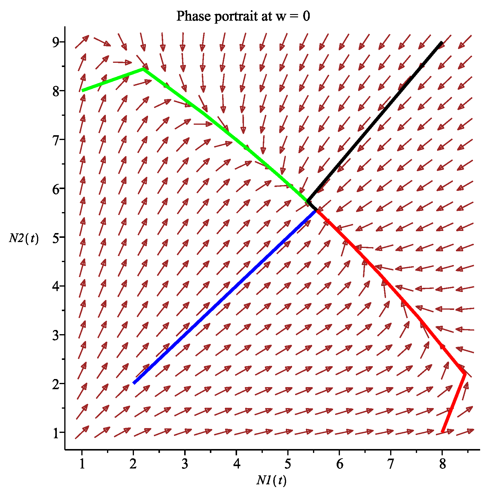
Figure A10.
Example 2 (): The positive equilibrium is globally asymptotically stable.
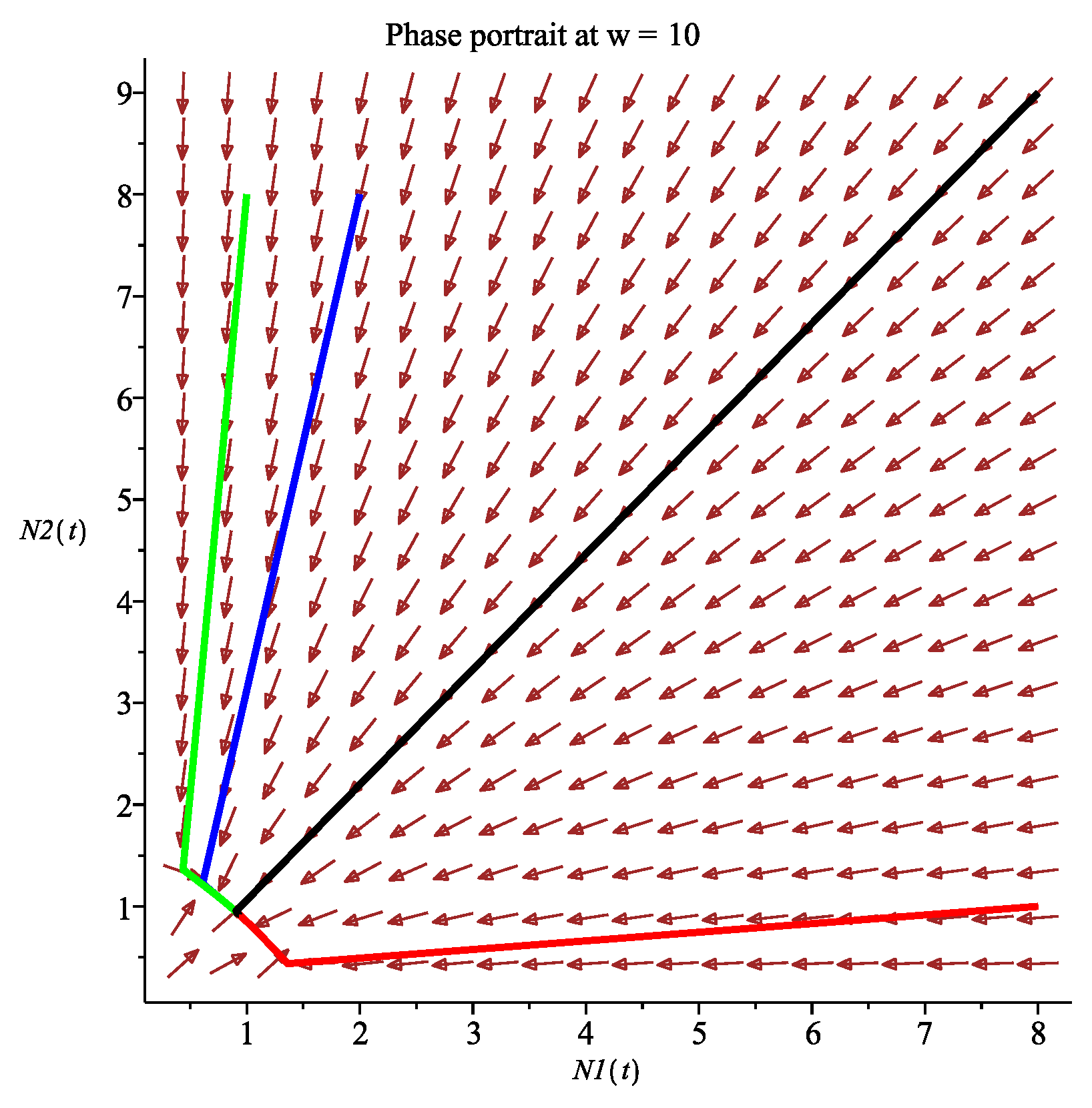
Figure A11.
Example 2 (): The boundary equilibrium is globally asymptotically stable.
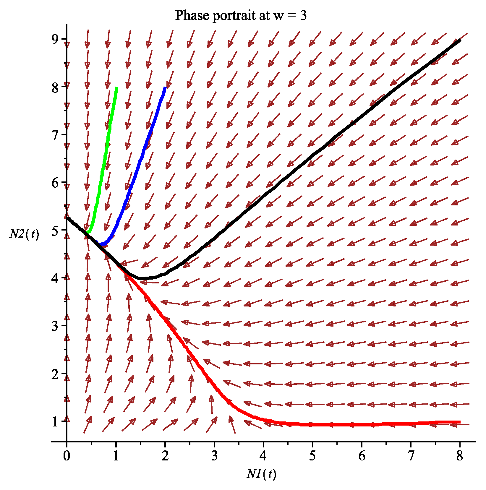
Figure A12.
Example 2 (): The boundary equilibrium is globally asymptotically stable.
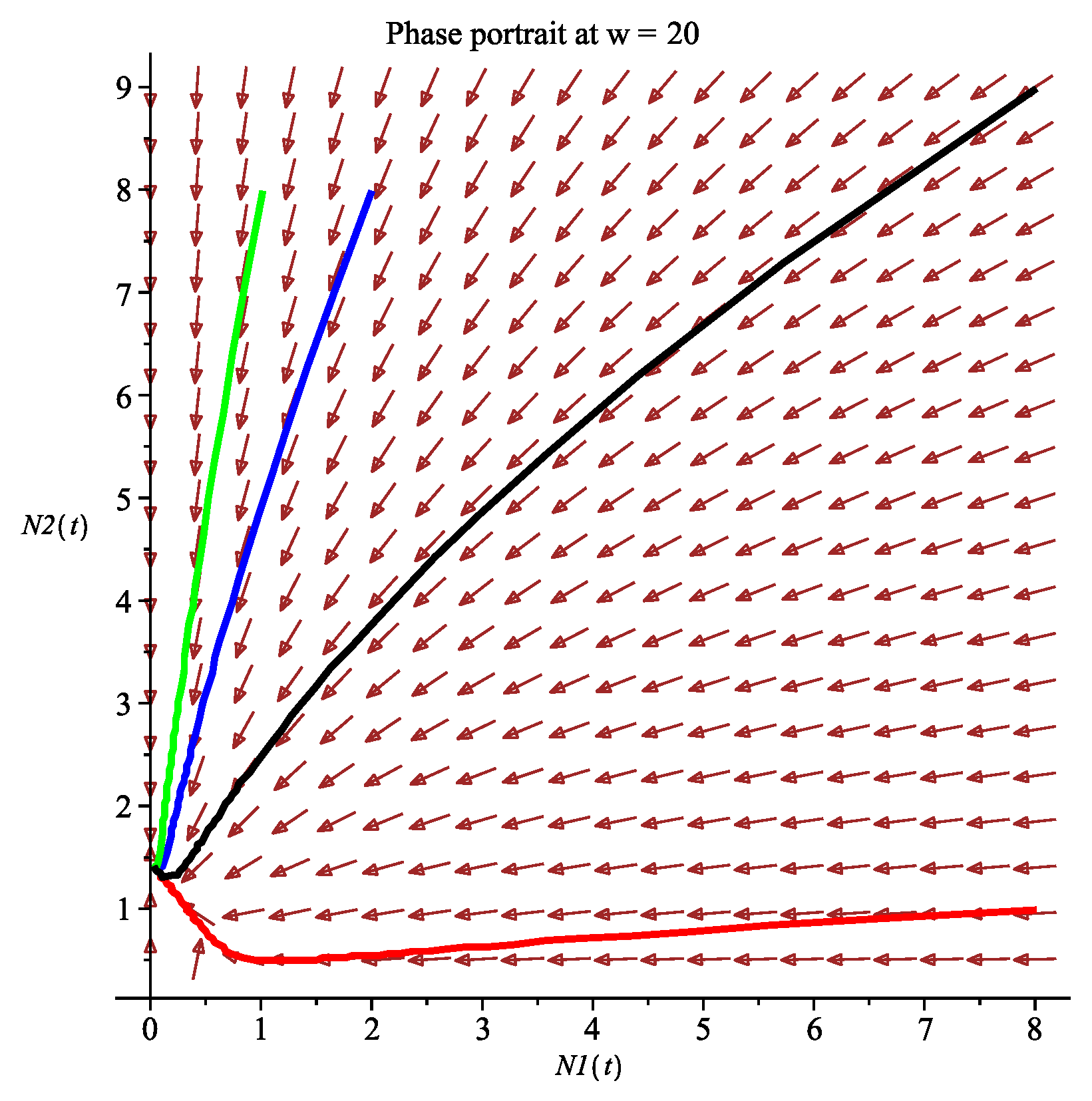
Figure A13.
Example 2, Case (1): Bifurcation diagram of the final equilibrium population densities versus wind speed.
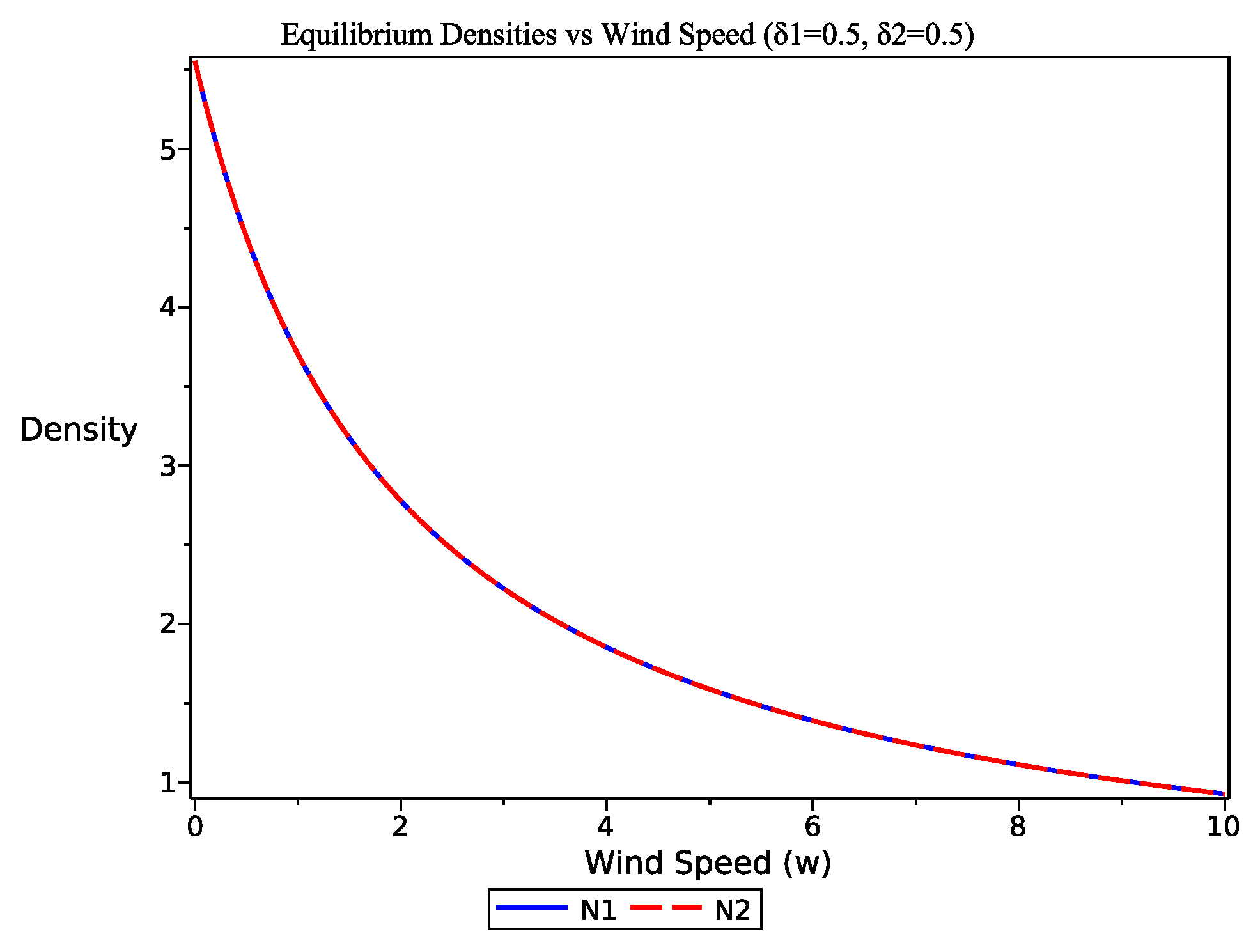
Figure A14.
Example 2, Case (2): Bifurcation diagram of the final equilibrium population densities versus wind speed.
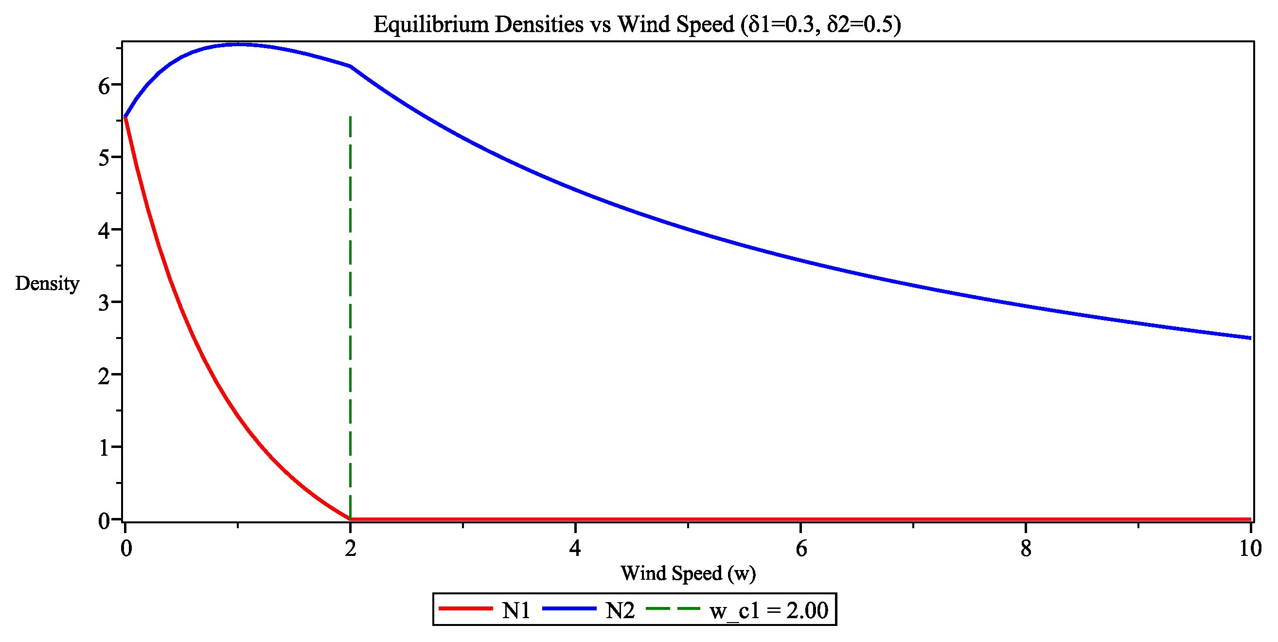
Figure A15.
Example 3 (): Bistable system dynamics.
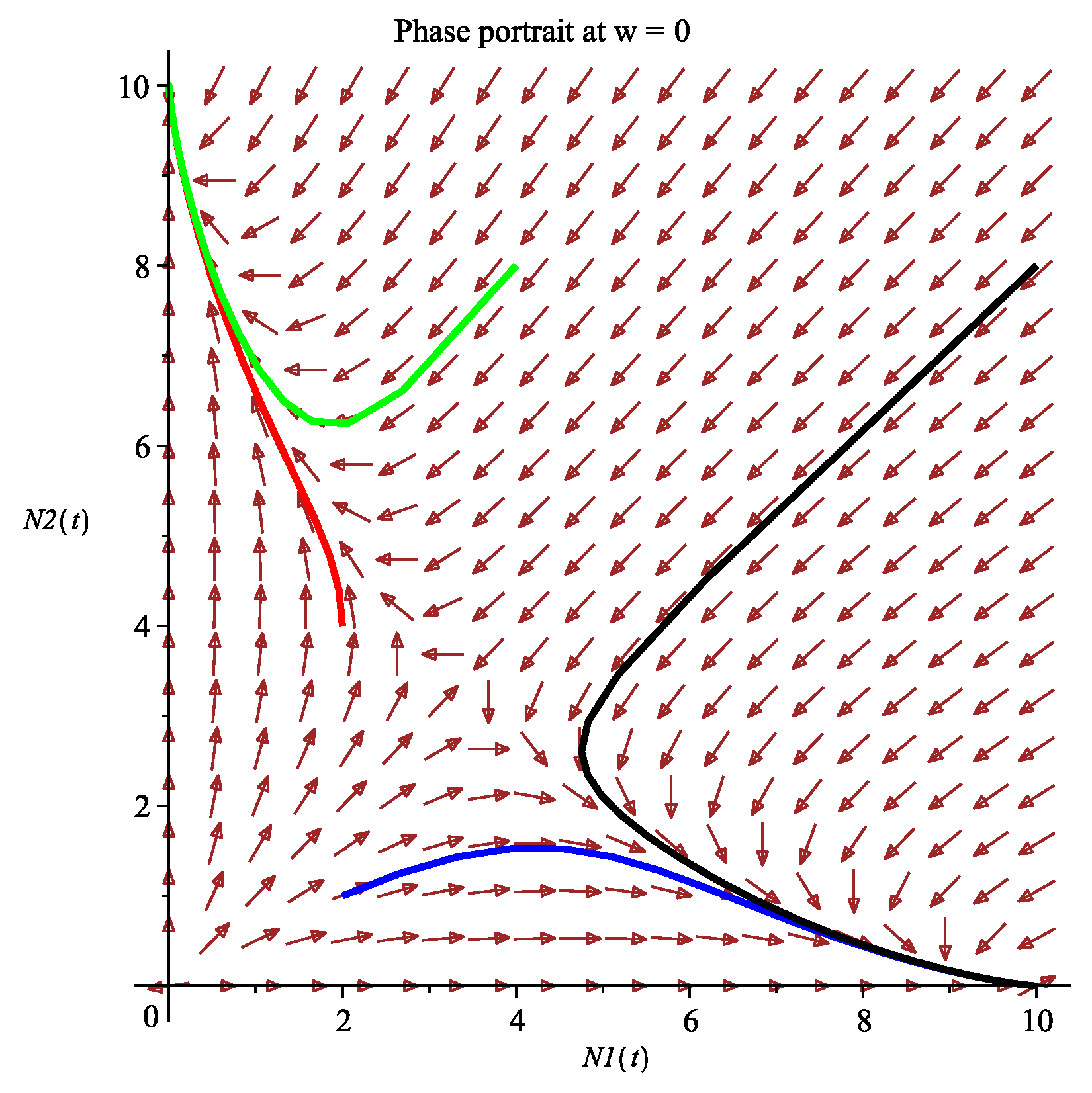
Figure A16.
Example 3 (): The boundary equilibria and are locally asymptotically stable.
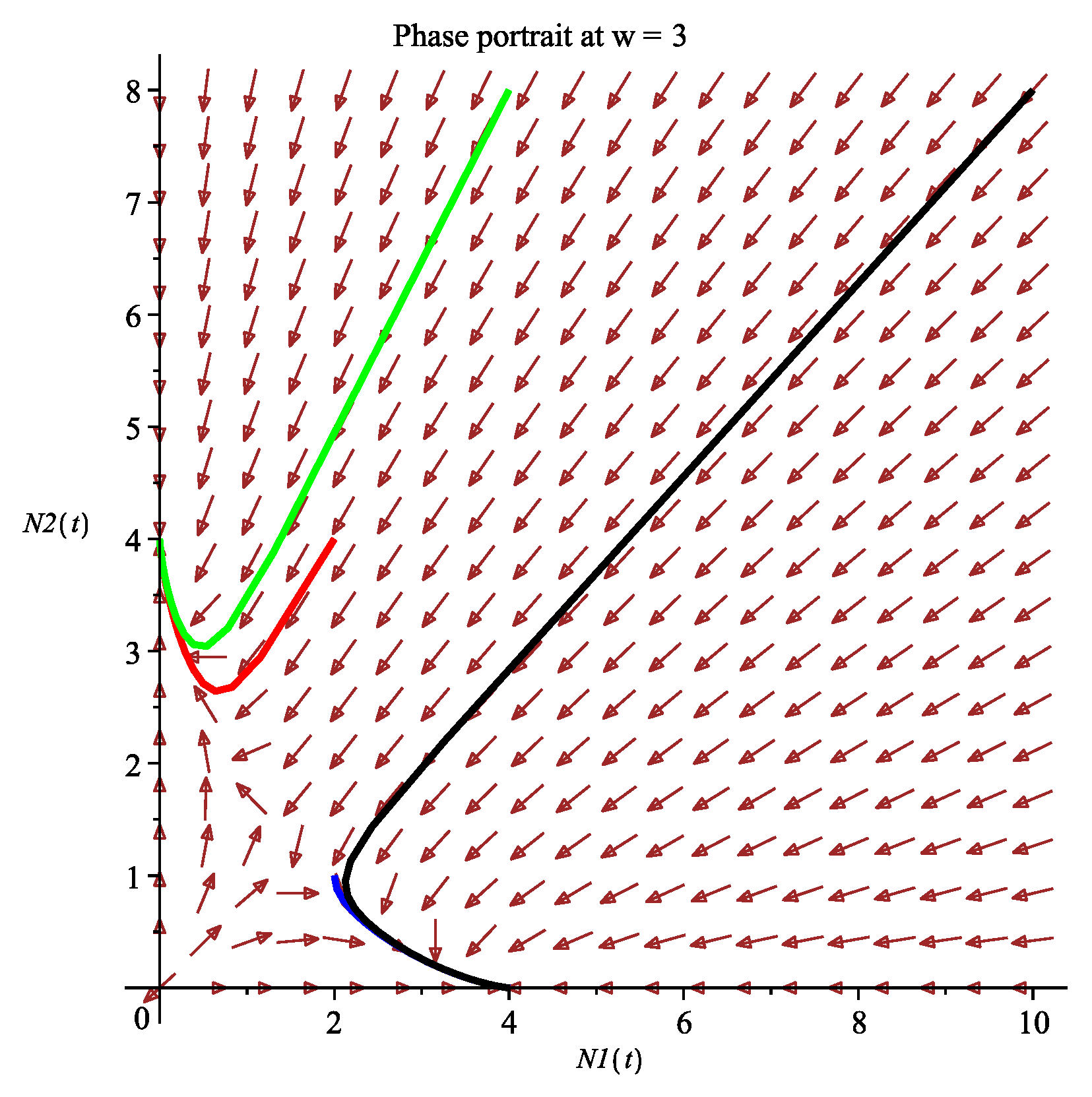
Figure A17.
Example 3 (), : The boundary equilibria and are locally asymptotically stable.
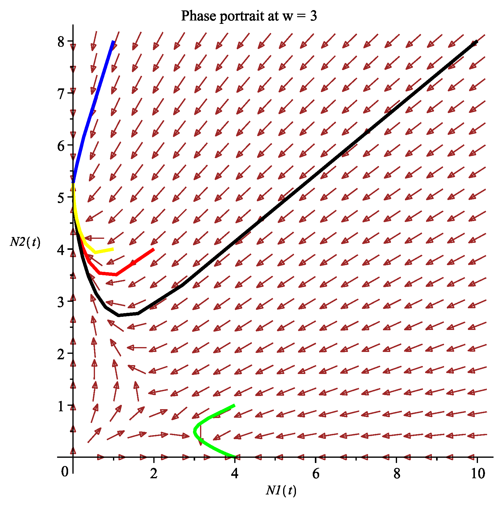
Figure A18.
Example 3 (), : The boundary equilibria and are locally asymptotically stable.
References
- Adler, P.B.; Smull, D.; Beard, K.H.; Choi, R.T.; Furniss, T.; Kulmatiski, A.; Meiners, J.M.; Tredennick, A.T.; Veblen, K.E. Competition and coexistence in plant communities: Intraspecific competition is stronger than interspecific competition. Ecol. Lett. 2018, 21, 1319–1329. [Google Scholar] [CrossRef] [Scilit] [PubMed]
- Grilli, J.; Barabás, G.; Michalska-Smith, M.J.; Allesina, S. Higher-order interactions stabilize dynamics in competitive network models. Nature 2017, 548, 210–213. [Google Scholar] [CrossRef] [Scilit] [PubMed]
- Cusumano, A.; Peri, E.; Colazza, S. Interspecific competition/facilitation among insect parasitoids. Curr. Opin. Insect Sci. 2016, 14, 12–16. [Google Scholar] [CrossRef] [Scilit] [PubMed]
- Alexander, J.M.; Diez, J.M.; Levine, J.M. Novel competitors shape species’ responses to climate change. Nature 2015, 525, 515–518. [Google Scholar] [CrossRef] [Scilit]
- Lou, Y.; Nie, H.; Wang, Y. Coexistence and bistability of a competition model in open advective environments. Math. Biosci. 2018, 306, 10–19. [Google Scholar] [CrossRef] [Scilit]
- Ghoul, M.; Mitri, S. The ecology and evolution of microbial competition. Trends Microbiol. 2016, 24, 833–845. [Google Scholar] [CrossRef] [Scilit]
- Zhu, Q.; Chen, F. Impact of fear on searching efficiency of first species: A two species Lotka-Volterra competition model with weak Allee effect. Qual. Theory Dyn. Syst. 2024, 23, 143. [Google Scholar] [CrossRef] [Scilit]
- De Silva, M.; Jang, S. Competitive exclusion and coexistence in a Lotka-Volterra competition model with Allee Effects and stocking. Lett. Biomath. 2015, 2, 56–66. [Google Scholar] [CrossRef]
- Wang, G.; Liang, X.-G.; Wang, F.-Z. The competitive dynamics of populations subject to an Allee effect. Ecol. Model. 1999, 124, 183–192. [Google Scholar] [CrossRef] [Scilit]
- Chen, S.; Chen, F.; Li, Z.; Chen, L. Bifurcation analysis of an allelopathic phytoplankton model. J. Biol. Syst. 2023, 31, 1063–1097. [Google Scholar] [CrossRef] [Scilit]
- Chen, L.; Chen, F. Extinction in a discrete Lotka-Volterra competitive system with the effect of toxic substances and feedback controls. Int. J. Biomath. 2015, 8, 1550012. [Google Scholar] [CrossRef] [Scilit]
- Huang, X.; Chen, F.; Xie, X.; Zhao, L. Extinction of a two species competitive stage-structured system with the effect of toxic substance and harvesting. Open Math. 2019, 17, 856–873. [Google Scholar] [CrossRef] [Scilit]
- Chen, S.; Chen, F.; Srivastava, V.; Parshad, R.D. Dynamical analysis of an allelopathic phytoplankton model with fear effect. Qual. Theory Dyn. Syst. 2024, 23, 189. [Google Scholar] [CrossRef] [Scilit]
- Chen, L.; Sun, J.; Chen, F.; Zhao, L. Extinction in a Lotka-Volterra competitive system with impulse and the effect of toxic substances. Appl. Math. Model. 2016, 40, 2015–2024. [Google Scholar] [CrossRef] [Scilit]
- Zhao, L.; Xie, X.; Yang, L.; Chen, F. Dynamic behaviors of a discrete Lotka-Volterra competition system with infinite delays and single feedback control. Abstr. Appl. Anal. 2014, 2014, 867313. [Google Scholar] [CrossRef] [Scilit]
- Chen, T.; Zhang, H.; Zhang, Y.; Wang, Z. Stochastic disturbances and delays drive coexistence and extinction in competing populations. Ecol. Model. 2025, 506, 111155. [Google Scholar] [CrossRef] [Scilit]
- Ma, C.; Zhang, X.; Yuan, R. Dynamic analysis of a stochastic regime-switching Lotka-Volterra competitive system with distributed delays and Ornstein-Uhlenbeck process. Chaos Solitons Fractals 2025, 190, 115765. [Google Scholar] [CrossRef] [Scilit]
- He, X.; Liu, Z. Partial permanence and stationary distribution of a stochastic competitive model with feedback controls and distributed delays. J. Appl. Math. Comput. 2022, 69, 1795–1818. [Google Scholar] [CrossRef] [Scilit]
- Wu, R.; Zou, X.; Wang, K. Dynamical behavior of a competitive system under the influence of random disturbance and toxic substances. Nonlinear Dyn. 2014, 77, 1209–1222. [Google Scholar] [CrossRef] [Scilit]
- Saenz, R.A.; Hethcote, H.W. Competing species models with an infectious disease. Math. Biosci. Eng. 2005, 3, 219–235. [Google Scholar] [CrossRef] [Scilit]
- Liechti, F. Birds: Blowin’ by the wind? J. Ornithol. 2006, 147, 202–211. [Google Scholar] [CrossRef] [Scilit]
- Srygley, R.B.; Dudley, R. Optimal strategies for insects migrating in the flight boundary layer: Mechanisms and consequences. Integr. Comp. Biol. 2008, 48, 119–133. [Google Scholar] [CrossRef] [Scilit] [PubMed]
- Shamoun-Baranes, J.; Liechti, F.; Vansteelant, W.M.G. Atmospheric conditions create freeways, detours and tailbacks for migrating birds. J. Comp. Physiol. A 2017, 203, 509–529. [Google Scholar] [CrossRef] [Scilit]
- Thorne, L.H.; Clay, T.A.; Phillips, R.A.; Silvers, L.G.; Wakefield, E.D. Effects of wind on the movement, behavior, energetics, and life history of seabirds. Mar. Ecol. Prog. Ser. 2023, 723, 73–117. [Google Scholar] [CrossRef] [Scilit]
- Masson-Delmotte, V.; Zhai, P.; Pirani, A.; Connors, S.L.; Pean, C.; Chen, Y.; Goldfarb, L.; Gomis, M.I.; Matthews, J.B.R.; Berger, S.; et al. Climate Change 2021: The Physical Science Basis. Contribution of Working Group I to the Sixth Assessment Report of the Intergovernmental Panel on Climate Change; Cambridge University Press: Cambridge, UK, 2021; 2391p. [Google Scholar]
- Drewitt, A.L.; Langston, R.H.W. Assessing the impacts of wind farms on birds. Ibis 2006, 148, 29–42. [Google Scholar] [CrossRef] [Scilit]
- Saidur, R.; Rahim, N.A.; Islam, M.R.; Solangi, K.H. Environmental impact of wind energy. Renew. Sustain. Energy Rev. 2011, 15, 2423–2430. [Google Scholar] [CrossRef] [Scilit]
- Huang, C.P.; Chen, F.D.; Zhu, Q.; Li, Q.Q. How the wind changes the Leslie-Gower predator-prey system? IAENG Int. J. Appl. Math. 2023, 53, 907–915. [Google Scholar]
- Cherry, M.J.; Barton, B.T. Effects of wind on predator-prey interactions. Food Webs 2017, 13, 92–97. [Google Scholar] [CrossRef] [Scilit]
- Barman, D.; Kumar, V.; Roy, J.; Alam, S. Modeling wind effect and herd behavior in a predator-prey system with spatiotemporal dynamics. Eur. Phys. J. Plus 2022, 137, 950–960. [Google Scholar] [CrossRef] [Scilit]
- Barman, D.; Roy, J.; Alam, S. Impact of wind in the dynamics of prey-predator interactions. Math. Comput. Simul. 2022, 191, 49–81. [Google Scholar] [CrossRef] [Scilit]
- Panja, P. Impacts of wind and anti-predator behaviour on predator-prey dynamics: A modelling study. Int. J. Comput. Sci. Math. 2022, 15, 396–407. [Google Scholar] [CrossRef] [Scilit]
- Thirthar, A.A.; Jawad, S.; Abbasi, M.A. The modified predator–prey model response to the effects of global warming, wind flow, fear, and hunting cooperation. Int. J. Dyn. Control 2025, 13, 3. [Google Scholar] [CrossRef] [Scilit]
- Pal, S.; Pal, N. Modelling the wind effect in predator–prey interactions. Math. Comput. Simul. 2025, 232, 75–90. [Google Scholar] [CrossRef] [Scilit]
- Dai, C.; Wang, Q.; Liu, Z.; Yan, Q. Trade-off dynamics of predator–prey system incorporating variable carrying capacity and wind effect. Chaos Solitons Fractals 2025, 199, 116594. [Google Scholar] [CrossRef] [Scilit]
- Chen, S.; Chen, F.; Srivastava, V.; Parshad, R.D. Dynamical analysis of a Lotka-Volterra competition model with both Allee and fear effects. Int. J. Biomath. 2024, 17, 2350077. [Google Scholar] [CrossRef] [Scilit]

Disclaimer/Publisher’s Note: The statements, opinions and data contained in all publications are solely those of the individual author(s) and contributor(s) and not of MDPI and/or the editor(s). MDPI and/or the editor(s) disclaim responsibility for any injury to people or property resulting from any ideas, methods, instructions or products referred to in the content. |
© 2026 by the authors. Licensee MDPI, Basel, Switzerland. This article is an open access article distributed under the terms and conditions of the Creative Commons Attribution (CC BY) license.