A Discrete Analogue of the Exponentiated Generalized Weibull-G Family: A New Discrete Distribution with Different Methods of Estimation and Application

Abstract

Statistical distributions play a crucial role in analyzing real data with varying behavior. In this study, the exponentiated generalized Weibull-G family is discretized using the survival discretization method. Furthermore, a three-parameter discrete distribution, called the exponentiated generalized Weibull–Rayleigh distribution, is generated from this discretized family. This distribution is flexible in modeling various data types, as evidenced by the distinct structures of its probability mass function and hazard rate function. Some statistical properties of both the family and the proposed distribution are discussed. Three estimation approaches—the maximum likelihood, the minimum chi-square, and the method of moments—are used to estimate the distribution’s parameters and are evaluated across three simulation cases. Moreover, the effectiveness of the proposed distribution is evaluated using four datasets from medicine and education. Overall, the results demonstrated the superiority of the proposed distribution fitting the examined data relative to some existing discrete models.

1. Introduction

Statistical distributions are highly significant for modeling real-world phenomena and informing decisions in urgent situations. It is notable that data behavior is becoming increasingly complex in the modern era, which motivates researchers to propose new distributions with high efficiency to model such sophisticated dynamics. Although extensive studies in the statistical literature have developed distributions with strong performance in modeling real data, most are continuous. Nevertheless, the data in many practical scenarios are captured in discrete units, which makes discrete distributions an essential approach for describing, analyzing, and modeling such data. Therefore, attention has been directed toward introducing new discrete distributions with high flexibility and adaptability for modeling phenomena with countable, distinct outcomes. Consequently, several techniques have been introduced to discretize existing continuous distributions, including hazard-rate-based, probability-density-function-based, survival-function-based, and moment-matching-based methods. For a comprehensive survey of different discretization methods, see [1]. However, the survival discretization method introduced by [2] is widely regarded as the most popular and widely applied in the literature. This method converts any continuous distribution to a discrete version using the survival function, thus maintaining the survival structure of its continuous counterpart and preserving key characteristics of the underlying continuous distribution. Let X be a random variable from any continuous distribution. The survival discretization method defines the probability mass function (PMF) of the discrete analogue as follows:

$$p(X=x)=S\left(x\right)-S(x+1);x=0,1,2,\dots ,$$

(1)

where $S\left(x\right)$ is the survival function of the continuous distribution. Subsequently, using this approach, researchers have introduced new discrete versions of well-known continuous distributions, such as the discrete Burr type XII and the discrete Lomax by [3], the discrete Gompertz–Weibul and discrete Gompertz exponential distribution by [4], the discrete Marshall–Olkin inverse Toppe–Leone distribution by [5], the discrete Burr–Hatke exponential distribution [6], the discrete Kumaraswamy erlang-truncated exponential distribution [7], the discrete power quasi-Xgamma [8], the discrete new XLindley distribution [9], and the discrete Weibull exponential distribution [10].

Moreover, various methodologies have been introduced in the literature to generate new distributions that model different types of continuous data. A well-established method in the literature is the exponentiated generalized (EG) method [11], which extends any distribution by adding two parameters to its cumulative distribution function (CDF). The EG method has the following CDF:

$$F(x,a,b,\mathsf{\eta })={\left[1-{\left[1-G(x,\mathsf{\eta })\right]}^a\right]}^b,$$

(2)

where $a>0$ and $b>0$ are shape parameters, and $\mathsf{\eta }$ is a vector of parameters for the base distribution. Another well-known method is the transformed–transformer (T-X) method proposed by [12]. This approach has been used by many authors to suggest new families of distributions. One widely used family introduced by utilizing the T-X method is the Weibull-G (W-G) family discussed by [13,14]. The CDF of the W-G family is expressed as follows:

$$G(x,c,\beta ,\mathsf{\zeta })=1-e^{-{\left({\displaystyle \frac{-log\left(1-H(x,\mathsf{\zeta })\right)}{\beta }}\right)}^c},$$

(3)

where $c>0$ and $\beta >0$ are the shape and scale parameters, respectively, and  $H(x,\mathsf{\zeta })$ is the CDF of the baseline distribution with vector of parameters $\mathsf{\zeta }$. In recent works by [15,16], the EG method and W-G family were combined, and new distributions, the exponentiated generalized Weibull–Rayleigh (EGWR) distribution and the exponentiated generalized Weibull exponential distribution, were introduced, respectively. The authors have demonstrated the strong ability of these distributions to model various forms of data. Moreover, additional approaches were proposed by researchers in an effort to generate new families of distributions, such as the beta-G method [17], the Kumaraswamy-G method [18], and the alpha-power method [19]. These methods have been used extensively in the literature and have demonstrated strong flexibility for modeling continuous. Because of the adaptability of the aforementioned families in fitting continuous data, researchers have suggested discrete analogues for these flexible families to broaden their use to a discrete scale, including the discrete Gompertz-G family by [4], the discrete analogue of the Weibull-G family by [20], the discrete analogue of the odd Weibull-G family by [21], the discrete exponential generalized-G family by [22], on the discretization of the Weibull-G by [10], and the discretization of the alpha power Weibull-G family by [23].

On the other hand, the Rayleigh distribution [24] is one of the most widely utilized continuous distributions due to its flexibility in modeling a wide range of data. This distribution has been extended by various authors in the literature. Some contributions can be found in [15,25,26,27,28,29], among others. Moreover, there has been an increasing focus on discretizing various extensions of the Rayleigh distribution. This can be seen in [30], who introduced the discrete Rayleigh (DR) distribution; ref. [31], who suggested the discrete inverse Rayleigh distribution; ref. [32], who proposed the discrete modified inverse Rayleigh distribution; ref. [33], who introduced the discrete Weibull–Rayleigh distribution; ref. [34], who studied the discrete exponentiated Marshall–Olkin Rayleigh (DEMOR); and ref. [35], who developed the discrete new generalized Rayleigh distribution (DNGR).

In this research, the main focus is to offer a discrete analogue of the exponentiated generalized Weibull-G (EGW-G) family, called the DEGW-G family, by utilizing the survival discretization method, and to derive and study a new discrete distribution, named the DEGW Rayleigh (DEGWR) distribution, as a member of this family. Despite the fact that the new family is formulated by using well-known distributional frameworks and a widely used survival discretization technique, the conceptual contribution resides in the structured integration of the EG framework with the Weibull-G approach prior to discretization to introduce the new discrete family. The new family falls into the broad framework of the discrete exponential generalized-G family [22] and is related to the previous work of [20,21]; however, its hierarchical structure of the parameters enhances the flexibility of the PMF and provides different forms of the hazard rate behavior. Thus, this research is motivated by the following aims:

• Enhance the literature by introducing a new discrete family of distributions in hopes of accurately representing different forms of discrete data.
• Provide a discrete version of the Rayleigh distribution with high ability in fitting left- and/or right-skewed data with low and/or high variability.
• Boost the flexibility of the probability mass function (PMF) and the hazard rate function (HRF) to accommodate varying data behavior, as shown by the plots of both functions.
• Offer greater adaptability in modeling count data compared to other existing discrete distributions.

This paper proceeds as follows: In Section 2, the DEGW-G family is presented with some statistical properties. Consequently, the DEGWR and its statistical properties with the stress–strength reliability analysis are introduced in Section 3 and Section 4, respectively. To estimate the distribution parameters, the maximum likelihood (ML) method, the minimum chi-square (MCS) method, and the method of moments (MM) are discussed in Section 5. To assess the performance of the three methods’ estimates, three simulation cases are explored in Section 6. To demonstrate the distribution’s efficiency, four datasets are analyzed in Section 7. Finally, Section 8 concludes the research.

2. Discrete Exponentiated Generalized Weibull-G Family

In this section, the DEGW-G family is introduced with some statistical properties. First. the new discrete family is derived from the continuous EGW-G family by applying the survival discretization method. Then, some key properties of the discrete family are discussed.

2.1. Discretization of the Exponentiated Generalized Weibull-G Family

The EGW-G family is acquired by combining the EG approach with the W-G family. Therefore, the CDF of the EGW-G family is constructed by substituting (3) into (2), and, hence, expressed in the following form:

$$F_{Cont.}\left(x\right)={\left[1-e^{-a{\left(-{\displaystyle \frac{log\left(1-H(x,\mathsf{\zeta })\right)}{\beta }}\right)}^c}\right]}^b,$$

(4)

with a survival function

$$S_{Cont.}\left(x\right)=1-{\left[1-e^{-a{\left(-{\displaystyle \frac{log\left(1-H(x,\mathsf{\zeta })\right)}{\beta }}\right)}^c}\right]}^b.$$

(5)

Thus, by utilizing the survival discretization method, the discrete analogue of the EGW-G family will be derived. Substituting (5) into (1), the DEGW-G family has the following PMF:

$$p_{Disc.}\left(x\right)={\left[1-e^{-a{\left({\displaystyle \frac{-log\left(1-H(x+1,\mathsf{\zeta })\right)}{\beta }}\right)}^c}\right]}^b-{\left[1-e^{-a{\left({\displaystyle \frac{-log\left(1-H(x,\mathsf{\zeta })\right)}{\beta }}\right)}^c}\right]}^b$$

(6)

Although the PMF is derived using the survival discretization method, it is qualitatively distinct from other discrete analogues constructed via the same technique. This is because the PMF is the difference between two power exponential terms, which yield hierarchical parameter effects. Therefore, the PMF exhibits diverse shapes. Therefore, the CDF, the survival, and the HRF for the DEGW-G family are, respectively, given by

$$F_{Disc.}\left(x\right)={\left[1-e^{-a{\left({\displaystyle \frac{-log\left(1-H(x+1,\mathsf{\zeta })\right)}{\beta }}\right)}^c}\right]}^b,$$

(7)

$$S_{Disc.}\left(x\right)=1-{\left[1-e^{-a{\left({\displaystyle \frac{-log\left(1-H(x,\mathsf{\zeta })\right)}{\beta }}\right)}^c}\right]}^b,$$

(8)

$$h_{Disc.}\left(x\right)={\displaystyle \frac{{\left[1-e^{-a{\left(\frac{-log\left(1-H(x+1,\mathsf{\zeta })\right)}{\beta }\right)}^c}\right]}^b-{\left[1-e^{-a{\left(\frac{-log\left(1-H(x,\mathsf{\zeta })\right)}{\beta }\right)}^c}\right]}^b}{1-{\left[1-e^{-a{\left(-\frac{log\left(1-H(x,\mathsf{\zeta })\right)}{\beta }\right)}^c}\right]}^b}}.$$

(9)

2.2. Statistical Properties of the DEGW-G Family

Examining statistical properties is fundamental to understanding the shape, tail, and variability for the data. This section examines properties of the DEGW-G family, including quantiles, moments, the moment-generating function, entropy, and order statistics.

2.2.1. Quantile Function

If X is a random variable from the DEGW-G family, then the quantile function is defined as

$$x_Q=min\left\{x\ge 0:F_{Disc.}\left(x\right)\ge u\right\}.$$

Thus, by inverting Equation (7), the quantile function is written as

$$x_Q=⌈H^{-1}\left(1-e^{-\beta {\left(-{\displaystyle \frac{1}{a}}log\left(1-u^{{\displaystyle \frac{1}{b}}}\right)\right)}^{{\displaystyle \frac{1}{c}}}};\mathsf{\zeta }\right)-1⌉,$$

(10)

where $\lceil .\rceil$ produces the smallest integer greater than or equal to its argument. As the CDF of the baseline distribution $H(.)$ is continuous and strictly increasing on its support, the inverse $H^{-1}(.)$ exists and is well-defined. Thereafter, for practical simulation purposes, the quantile is calculated for $u\in (0,1)$ and the parameter values $a>0,b>0,c>0,\mathrm{and}\beta >0$, which ensure that the argument of the inverse $H^{-1}(.)$ lies in the interval $(0,1)$.

2.2.2. Moments

The rth moment of the DEGW-G family is expressed as follows:

$${\mu }_r=E\left(x^r\right)=\sum _{x=0}^{\infty }{x}^r{p}_{Disc.}\left(x\right)=\sum _{x=1}^{\infty }\left(x^r-{(x-1)}^r\right)S_{Disc.}\left(x\right).$$

Letting $r=1$ and 2 yield the mean and variance of the DEGW-G family, respectively.

2.2.3. Moment-Generating Function

The moment-generating function for the DEGW-R family is constructed as

$$M{G}_x\left(t\right)=E\left(e^{tx}\right)=\sum _{x=0}^{\infty }{e}^{tx}{p}_{Disc.}\left(x\right)=1+\left(1-e^{-t}\right)\sum _{x=1}^{\infty }{e}^{tx}{S}_{Disc.}\left(x\right).$$

In the expressions of the moment and moment-generating function, convergence is determined by the tail behavior of $S_{Disc.}\left(x\right)$, which is influenced by the asymptotic behavior of the baseline distribution $H\left(x\right)$. Consequently, a sufficient tail decay will guarantee the existence of finite-order moments and will determine the domain of convergence of the moment-generating function.

2.2.4. Rényi and Shannon Entropy

Entropy is a measure of uncertainty and complexity for a random variable and is widely applied in statistical theory. Rényi entropy [36] is expressed as

$$R_{\gamma }\left(x\right)={\displaystyle \frac{1}{1-\gamma }}log\sum _{x=0}^{\infty }{\left[p_{Disc.}\left(x\right)\right]}^{\gamma },\gamma >0,\gamma \ne 1.$$

Moreover, Shannon entropy [37] is formulated as

$$SH\left(x\right)=-E\left[log{p}_{Disc.}\left(x\right)\right]=-\sum _{x=0}^{\infty }{p}_{Disc.}\left(x\right)log{p}_{Disc.}\left(x\right).$$

2.2.5. Order Statistics

Let $x_1,x_2,\dots ,x_n$ be a sample randomly taken from the DEGW-G family with order statistics $x_{1:n},x_{2:n},\dots ,x_{n:n}$. The CDF for the sth order statistics is defined as

$$F_{s:n}\left(x\right)=\sum _{k=s}^n\left(\begin{array}{c}n\\ k\end{array}\right)F_{Disc.}{\left(x\right)}^k{\left(1-F_{Disc.}\left(x\right)\right)}^{n-k}.$$

Using the binomial expansion

$${\left(1-z\right)}^{n-k}=\sum _{j=0}^{n-k}{(-1)}^j\left(\begin{array}{c}n-k\\ j\end{array}\right)z^j,$$

where $n-k$ is a non-negative integer; therefore,

$$F_{s:n}\left(x\right)=\sum _{k=s}^n\sum _{l=0}^{n-k}{(-1)}^l\left(\begin{array}{c}n-k\\ l\end{array}\right)\left(\begin{array}{c}n\\ k\end{array}\right)F_{Disc.}{\left(x\right)}^{k+l}.$$

(11)

In addition, the PMF of the above CDF is defined by [38] and, hence, is given by

$$p_{s:n}\left(x\right)=F_{s:n}\left(x\right)-F_{s:n}(x-1).$$

3. A Special Member: The DEGWR Distribution

In this section, a member of the DEGW-G family is introduced by using the Rayleigh distribution as a baseline distribution. Let X be a random variable from the Rayleigh distribution; then, the CDF is written as

$$H(x,\sigma )=1-e^{-{\displaystyle \frac{x^2}{2{\sigma }^2}}},$$

(12)

where $\sigma >0$ is the shape parameter. Substituting (12) into (6), the DEGWR distribution has the subsequent PMF:

$$p\left(x\right)={\left[1-e^{-a{\left({\displaystyle \frac{{(x+1)}^2}{2{\sigma }^2\beta }}\right)}^c}\right]}^b-{\left[1-e^{-a{\left({\displaystyle \frac{x^2}{2{\sigma }^2\beta }}\right)}^c}\right]}^b.$$

(13)

After re-parametrization, for notation simplicity, the PMF for the DEGWR distribution can be rewritten as

$$p\left(x\right)={\left[1-q^{{(x+1)}^{2c}}\right]}^b-{\left[1-q^{x^{2c}}\right]}^b,$$

(14)

where $0<q=e^{-a{\left({\displaystyle \frac{1}{2{\sigma }^2\beta }}\right)}^c}<1$. It is clear that the parameter q is a function of the original parameters $(a,\beta ,\sigma )$, thereby combining their scale/rate effects in the discrete formulation. Thus, q contributes directly to the decay behavior of the discrete PMF. Accordingly, the CDF, survival, and HRF are, respectively, defined as

$$F\left(x\right)={\left[1-q^{{(x+1)}^{2c}}\right]}^b,$$

(15)

$$S\left(x\right)=1-{\left[1-q^{{\left(x\right)}^{2c}}\right]}^b,$$

(16)

$$h\left(x\right)={\displaystyle \frac{{\left[1-q^{{(x+1)}^{2c}}\right]}^b-{\left[1-q^{x^{2c}}\right]}^b}{1-{\left[1-q^{{\left(x\right)}^{2c}}\right]}^b}}.$$

(17)

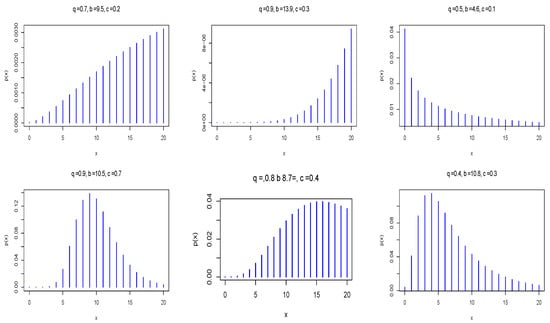
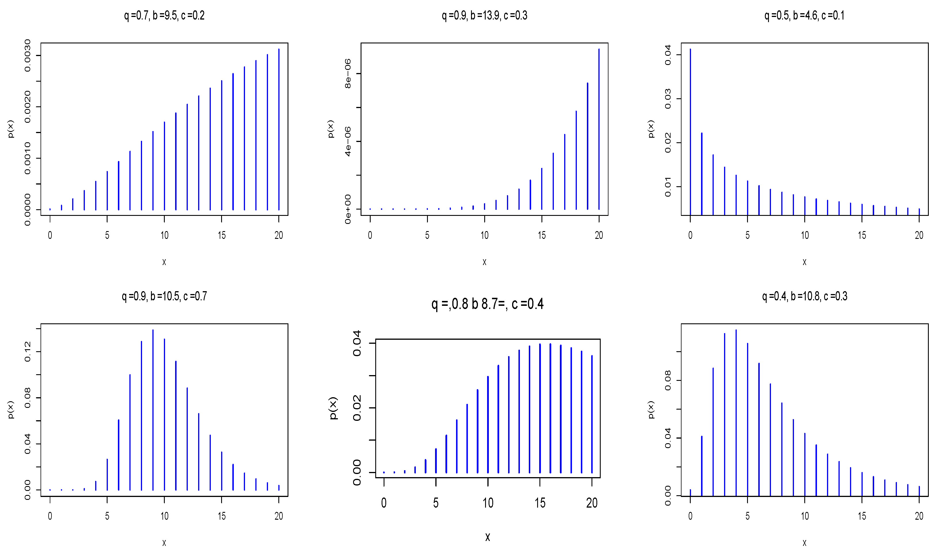
Various forms of the PMF with different parameter values are given in Figure 1. As is evident, the PMF exhibits patterns such as increasing, decreasing, J-shaped, skewed, and symmetric, which make it flexible for modeling different behaviors of discrete data across many fields.

Figure 1. The PMF of the DEGWR distribution with different parameters.

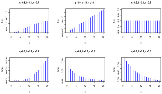
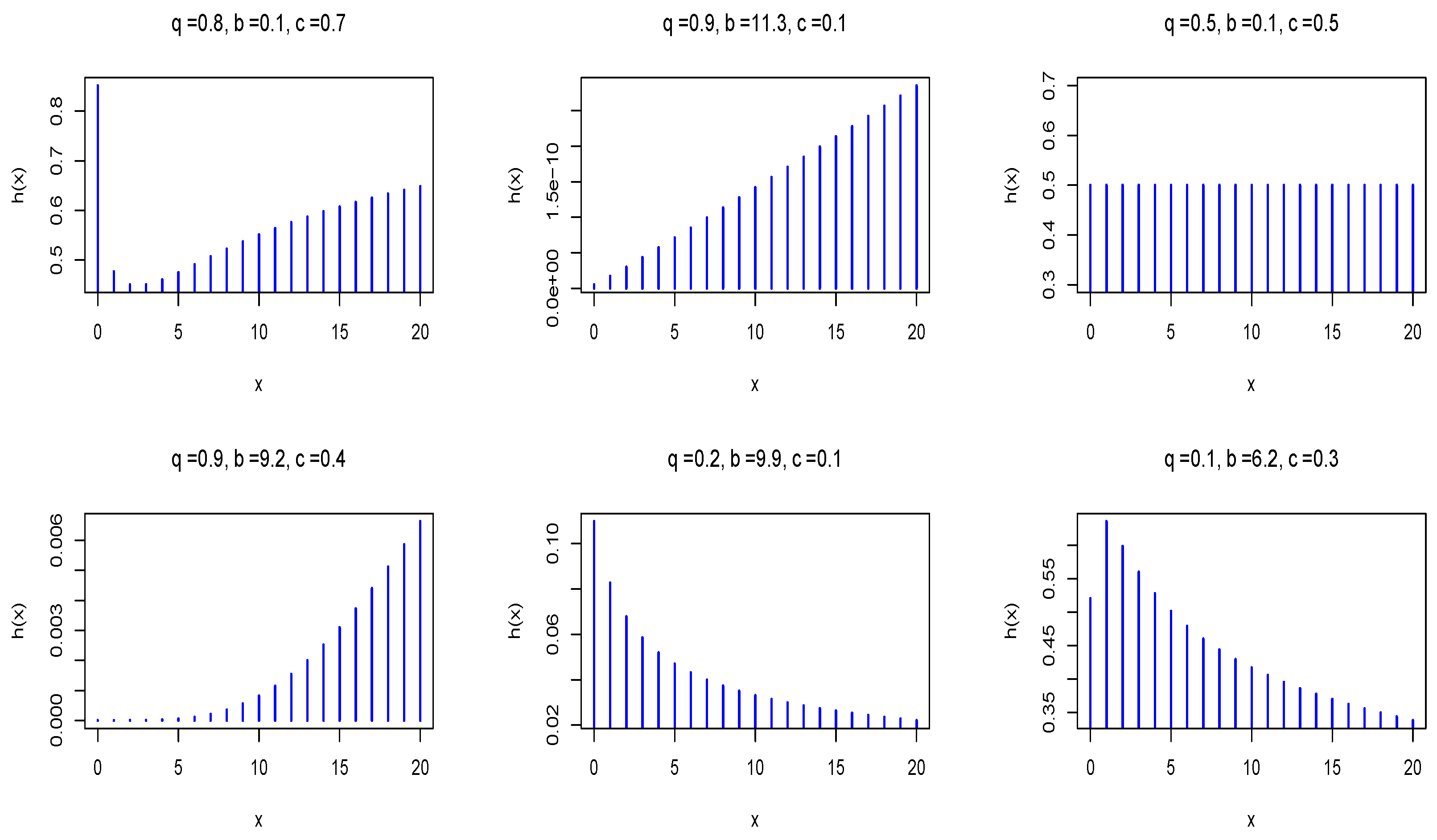
Figure 2 shows various hazard rate patterns, including increasing, when the hazard rate rises monotonically with x; decreasing, when it declines monotonically with x; and bathtub-shaped, when it exhibits an incline following a decline. These patterns are controlled by the combined effect of the parameters q, b, and c. More precisely, different combinations of the parameters yield different patterns of the HRF.

Figure 2. The HRF of the DEGWR distribution with different parameters.

4. Statistical Properties and Reliability Analysis of the DEGWR Distribution

This section summarizes some statistical properties and the stress–strength reliability for the DEGWR distribution.

4.1. Quantile Function

The quantile function for the DEGWR distribution is described by the inverse of (15). Hence, if X is a random variable from the DEGWR distribution, the quantile function is formulated as

$$x_Q=⌈{\left\{{\displaystyle \frac{1}{log\left(q\right)}}\left[log(1-u^{{\displaystyle \frac{1}{b}}})\right]\right\}}^{{\displaystyle \frac{1}{2c}}}-1⌉,$$

where $u\in (0,1)$, and different values of u provide different quantiles. Hence, the median is then given by

$$x_{0.5}=⌈{\left\{{\displaystyle \frac{1}{log\left(q\right)}}\left[log(1-{0.5}^{{\displaystyle \frac{1}{b}}})\right]\right\}}^{{\displaystyle \frac{1}{2c}}}-1⌉.$$

4.2. Moments

For the random variable X from the DEGWR distribution, the rth moment is summarized as

$${\mu }_r=\sum _{x=1}^{\infty }\left(x^r-{(x-1)}^r\right)S\left(x\right)=\sum _{x=1}^{\infty }\left(x^r-{(x-1)}^r\right)\left\{1-{\left[1-q^{x^{2c}}\right]}^b\right\}.$$

Therefore, the mean ($\mu$), variance (${\sigma }^2$), coefficient of variation (COV), and dispersion index (DI) are, respectively, given by

$$\begin{array}{cc}\hfill \mu & =\sum _{x=1}^{\infty }\left[1-{\left(1-q^{x^{2c}}\right)}^b\right],\hfill \\ \hfill {\sigma }^2& ={\mu }_2-{\mu }_1^2=\sum _{x=1}^{\infty }\left(2x-1\right)\left[1-{\left(1-q^{x^{2c}}\right)}^b\right]-{\left\{\sum _{x=1}^{\infty }\left[1-{\left(1-q^{x^{2c}}\right)}^b\right]\right\}}^2,\hfill \\ \hfill COV& ={\displaystyle \frac{\sigma }{\mu }}={\displaystyle \frac{{\left\{{\displaystyle \sum _{x=1}^{\infty }}\left(2x-1\right)\left[1-{\left(1-q^{x^{2c}}\right)}^b\right]-{\left\{{\displaystyle \sum _{x=1}^{\infty }}\left[1-{\left(1-q^{x^{2c}}\right)}^b\right]\right\}}^2\right\}}^{1/2}}{{\displaystyle \sum _{x=1}^{\infty }}\left[1-{\left(1-q^{x^{2c}}\right)}^b\right]}},\hfill \\ \hfill DI& ={\displaystyle \frac{{\sigma }^2}{\mu }}={\displaystyle \frac{{\displaystyle \sum _{x=1}^{\infty }}\left(2x-1\right)\left[1-{\left(1-q^{x^{2c}}\right)}^b\right]-{\left\{{\displaystyle \sum _{x=1}^{\infty }}\left[1-{\left(1-q^{x^{2c}}\right)}^b\right]\right\}}^2}{{\displaystyle \sum _{x=1}^{\infty }}\left[1-{\left(1-q^{x^{2c}}\right)}^b\right]}}.\hfill \end{array}$$

Moreover, the skewness (SK), a measure of shape, and the Kurtosis (K), a measure of peakness and tailedness, can be obtained by using the first four moments as follows:

$$\begin{array}{cc}\hfill SK& ={\displaystyle \frac{{\mu }_3-3{\mu }_2{\mu }_1+2{\mu }_1^3}{{({\mu }_2-{\mu }_1^2)}^{\frac{3}{2}}}},\hfill \\ \hfill K& ={\displaystyle \frac{{\mu }_4-4{\mu }_3{\mu }_1+6{\mu }_2{\mu }_1^2-3{\mu }_1^4}{{({\mu }_2-{\mu }_1^2)}^2}}.\hfill \end{array}$$

The aforementioned measures can be calculated using R statistical software. Table 1 shows the results for the following cases of parameters:

$$\begin{array}{cc}\hfill & \mathbf{I}:q=0.9,b=0.7,c=3.4.\hfill \\ \hfill & \mathbf{II}:q=0.1,b=4.0,c=5.9.\hfill \\ \hfill & \mathbf{III}:q=0.3,b=2.7,c=1.5.\hfill \\ \hfill & \mathbf{IV}:q=0.8,b=0.2,c=1.3.\hfill \\ \hfill & \mathbf{V}:q=0.6,b=2.4,c=2.6.\hfill \\ \hfill & \mathbf{VI}:q=0.9,b=2.7,c=0.8.\hfill \end{array}$$

Table 1. Results of the mean, variance, COV, DI, SK, and K for the above cases.

	Mean	Variance	COV	DI	SK	K
I	0.800479	0.159723	0.499268	0.199535	−1.503488	3.261350
II	0.343900	0.225633	1.381239	0.656100	0.657252	1.431980
III	0.618440	0.236326	0.786065	0.382133	−0.483011	1.245966
IV	0.337271	0.355930	1.768900	1.055323	1.698173	5.283869
V	0.889097	0.098604	0.353181	0.110903	−2.478226	7.141611
VI	1.751096	7.393041	1.552750	4.221951	1.671346	5.108751

In Table 1, the dispersion index shows flexibility in modeling over-dispersed and under-dispersed data. The distribution’s adaptability accommodates numerous asymmetric data types, ad demonstrated by its ability to be left- or right-skewed (positively or negatively). Finally, the kurtosis values indicate that the distribution is effective at modeling data with either sharp peaks and heavier tails or flat peaks and lighter tails, thereby demonstrating that it can be leptokurtic or platykurtic.

4.3. Moment-Generating Function

Let X be a random variable from the DEGWR distribution; then the moment-generating function of X can be outlined as

$$G_x\left(t\right)=1+\left(1-e^{-t}\right)\sum _{x=1}^{\infty }{e}^{tx}S\left(x\right)=1+\left(1-e^{-t}\right)\sum _{x=1}^{\infty }{e}^{tx}\left[1-{\left(1-q^{x^{2c}}\right)}^b\right].$$

4.4. Rényi and Shannon Entropy

Rényi entropy and Shannon entropy are, respectively, characterized by

$$R_{\gamma }\left(x\right)={\displaystyle \frac{1}{1-\gamma }}log\sum _{x=0}^{\infty }{\left[{\left(1-q^{{(x+1)}^{2c}}\right)}^b-{\left(1-q^{x^{2c}}\right)}^b\right]}^{\gamma },\gamma >0,\gamma \ne 1,$$

$$SH\left(x\right)=-\sum _{x=0}^{\infty }\left[{\left(1-q^{{(x+1)}^{2c}}\right)}^b-{\left(1-q^{x^{2c}}\right)}^b\right]log\left[{\left(1-q^{{(x+1)}^{2c}}\right)}^b-{\left(1-q^{x^{2c}}\right)}^b\right].$$

4.5. Order Statistics

From Equations (11) and (15), the CDF of the sth-order statistic for the random sample $x_1,x_2,\dots ,x_n$, from the DEGWR distribution, takes the form

$$F_{s:n}\left(x\right)=\sum _{k=s}^n\sum _{l=0}^{n-k}{(-1)}^l\left(\begin{array}{c}n-k\\ l\end{array}\right)\left(\begin{array}{c}n\\ k\end{array}\right){\left(1-q^{{(x+1)}^{2c}}\right)}^{b(k+l)-1}.$$

(18)

Applying the following expansion,

$${\left(1-y\right)}^{\eta }=\sum _{m=0}^{\infty }{(-1)}^m\left(\begin{array}{c}\eta -1\\ m\end{array}\right)y^m,$$

where $0<y<1$ and $\eta >0$, then

$$F_{s:n}\left(x\right)=\sum _{m=0}^{\infty }\sum _{k=s}^n\sum _{l=0}^{n-k}{(-1)}^{l+m}\left(\begin{array}{c}b(k+l)-1\\ m\end{array}\right)\left(\begin{array}{c}n-k\\ l\end{array}\right)\left(\begin{array}{c}n\\ k\end{array}\right)q^{m{(x+1)}^{2c}}.$$

Moreover, the PMF of the sth order statistic is defined by

$$p_{s:n}\left(x\right)=\sum _{m=0}^{\infty }\sum _{k=s}^n\sum _{l=0}^{n-k}{(-1)}^{l+m}\left(\begin{array}{c}b(k+l)-1\\ m\end{array}\right)\left(\begin{array}{c}n-k\\ l\end{array}\right)\left(\begin{array}{c}n\\ k\end{array}\right)\left(q^{m{(x+1)}^{2c}}-q^{m{\left(x\right)}^{2c}}\right).$$

4.6. Stress–Strength Reliability Analysis

Stress–strength reliability is a measure of the ability of a system to function without failure. It is of great interest across disciplines such as medicine, engineering, and computer infrastructure. System failure occurs when stress exceeds strength. Therefore, assuming that $X_S$ and $X_{S^{\ast }}$ are random variables representing stress and strength, respectively, stress–strength reliability $\left(R\right)$ is defined as follows:

$$\begin{array}{c}\hfill R=P(X_S\le X_{S^{\ast }})=\sum _{x=0}^{\infty }{p}_{X_S}\left(x\right)S_{X_{S^{\ast }}}\left(x\right).\end{array}$$

Now, let $X_S\sim \mathrm{DEGWR}(q_1,b_1,c_1)$ and $X_{S^{\ast }}\sim \mathrm{DEGWR}(q_2,b_2,c_2)$; then, R can be expressed as

$$\begin{array}{c}\hfill R=\sum _{x=0}^{\infty }\left\{{\left[1-q_1^{{(x+1)}^{2c_1}}\right]}^{b_1}-{\left[1-q_1^{x^{2c_1}}\right]}^{b_1}\right\}\left\{1-{\left[1-q_2^{x^{2c_2}}\right]}^{b_2}\right\}.\end{array}$$

As the PMF and the survival function involve nonlinear transformations, a closed-form expression for stress–strength reliability is not attainable. Thus, numerical computations using R statistical software are performed to evaluate the stress–strength reliability measure, as is standard practice. Table 2 displays the values of R for some cases of parameters.

Table 2. Values of stress–strength reliability for a selection of parameter values.

Case	Stress	Strength	$\mathit{R}=\mathit{P}(\mathit{X}<\mathit{Y})$	Remarks
I	$(0.85,5,2)$	$(0.35,2,2)$	0.4475	Low–moderate reliability
II	$(0.75,1.4,5)$	$(0.75,1.4,2)$	0.8125	High reliability
III	$(0.35,2,1)$	$(0.85,5,1)$	0.9475	Very high reliability
IV	$(0.85,3,1)$	$(0.05,2,2)$	0.1924	Very low reliability
V	$(0.90,6,2)$	$(0.25,2,2)$	0.3250	Low reliability
VI	$(0.75,3,1.5)$	$(0.55,3,1.5)$	0.6625	Moderate reliability

Table 2 demonstrates the ability and flexibility of the DEGWR distribution in modeling different levels of reliability. Accordingly, it is applicable to various fields, including reliability engineering, risk analysis, and system lifetimes.

5. Parameter Estimation

In this section, classical estimation methods, the ML, MCS, and MM approaches, are implemented to improve the robustness and accuracy of estimates of the DEGWR distribution parameters.

5.1. Maximum Likelihood Method

The ML method is widely used for estimating statistical distributions. It depends on maximizing the likelihood of observing the sample under the assumed distribution and has several properties, such as consistency and unbiasedness in large samples. It is an invaluable method of estimation due to its ability to incorporate complex distributions. Let $x_1,x_2,\dots ,x_n$ be a random sample from the DEGWR distribution; the log likelihood function is defined as

$$\mathsf{\ell }=\sum _{x=1}^{\infty }log\left[{\left(1-q^{{(x+1)}^{2c}}\right)}^b-{\left(1-q^{{\left(x\right)}^{2c}}\right)}^b\right].$$

(19)

The distribution parameters can be estimated by equating the first derivative of Equation (19), with respect to each parameter, to zero and solving them iteratively using, for example, the Newton–Raphson technique. Another method for estimating the distribution’s parameters is to maximize Equation (19) directly using any optimization method, such as the optim The following highlights are the same. function in the R statistical package (version 4.3.2).

5.2. Minimum Chi-Square Method

The MSC method is proposed by [39] as an alternative to the ML approach. It depends on minimizing the discrepancy between the observed frequencies and expected ones under the assumed distribution. It is appropriate when the data are discrete or aggregated into classes (for more details, see [40] and references therein). Let $k\in \{0,1,2,\dots \}$ be the possible values, with $O_k$ and $p_k$ being the corresponding observed frequencies and the probabilities provided based on the DEGWR distribution, respectively. Accordingly, the unknown parameters are estimated by minimizing the following discrepancy measure:

$$\begin{array}{c}\hfill {\chi }^2=\sum _k{\displaystyle \frac{{(O_k-n{p}_k)}^2}{n{p}_k}},\end{array}$$

(20)

where $p_k$ corresponds to the PMF, as given in Equation (14), evaluated at k. The minimization of Equation (20) can be achieved by using the optimization function optim in R.

5.3. Method of Moment

The MM is among the earliest approaches reported in the literature for parameter estimation. It is formulated by equating the first three theoretical moments, i.e., ${\mu }_1(q,b,c)=E\left(X\right)$, ${\mu }_2(q,b,c)=E\left(X^2\right)$, and ${\mu }_3(q,b,c)=E\left(X^3\right)$, with the empirical moments ${\widehat{\mu }}_1$, ${\widehat{\mu }}_2$, and ${\widehat{\mu }}_3$ obtained from the sample. To obtain a closed-form solution to this system of nonlinear equations, numerical optimization is required [41]. Therefore, the estimates of the DEGWR distribution’s parameters can be derived by minimizing the following quadratic function:

$$\begin{array}{c}\hfill Q\left(x\right)={\left({\mu }_1(q,b,c)-{\widehat{\mu }}_1\right)}^2+{\left({\mu }_2(q,b,c)-{\widehat{\mu }}_2\right)}^2+{\left({\mu }_3(q,b,c)-{\widehat{\mu }}_3\right)}^2\end{array}$$

(21)

Minimizing Equation (21) by employing any optimization function, such as optim, provides the estimates of parameters.

6. Simulation Study

To assess the efficiency of the ML, MCS, and MM methods in accurately estimating the parameters of the DEGWR distribution, three simulation cases are introduced. For each case, different sample sizes, $n=(25,50,100,300,500)$, are used with the number of simulations $m=5000$. The true values of the parameters for the three cases are as follows:

$$\begin{array}{cc}\hfill & \mathbf{Case}\mathbf{I}:q=0.3,b=5.8,c=1.2.\hfill \\ \hfill & \mathbf{Case}\mathbf{II}:q=0.6,b=2.9,c=1.6.\hfill \\ \hfill & \mathbf{Case}\mathbf{III}:q=0.8,b=1.6,c=2.1.\hfill \end{array}$$

To evaluate the accuracy of the estimates produced by the three methods, the mean squared error (MSE) and the mean absolute error (MAE) are used. These measures are obtained, respectively as follows:

$$\begin{array}{cc}\hfill \mathrm{MSE}\left(\widehat{\mathsf{\Lambda }}\right)& =\sum _{i=1}^m{\displaystyle \frac{{({\widehat{\mathsf{\Lambda }}}_i-{\mathsf{\Lambda }}_{tr})}^2}{m}},\hfill \end{array}$$

$$\begin{array}{cc}\hfill \mathrm{MAE}\left(\widehat{\mathsf{\Lambda }}\right)& =\sum _{i=1}^m{\displaystyle \frac{|{\widehat{\mathsf{\Lambda }}}_i-{\mathsf{\Lambda }}_{tr}|}{m}},\hfill \end{array}$$

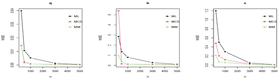
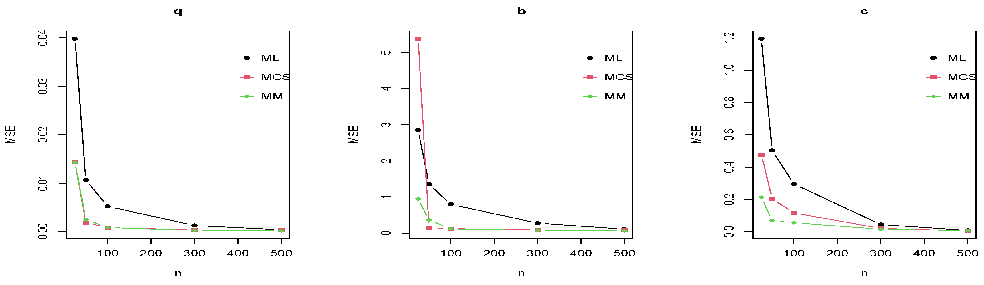
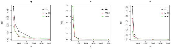
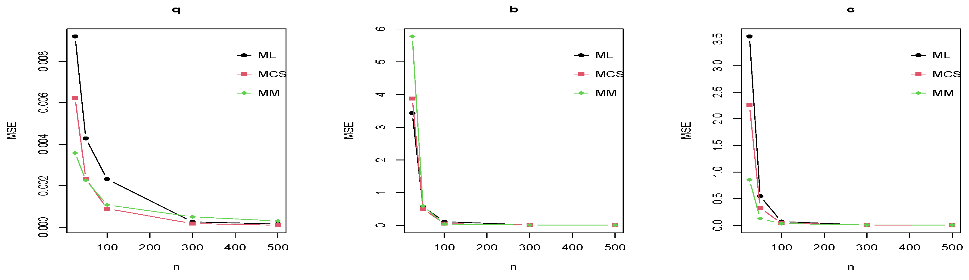
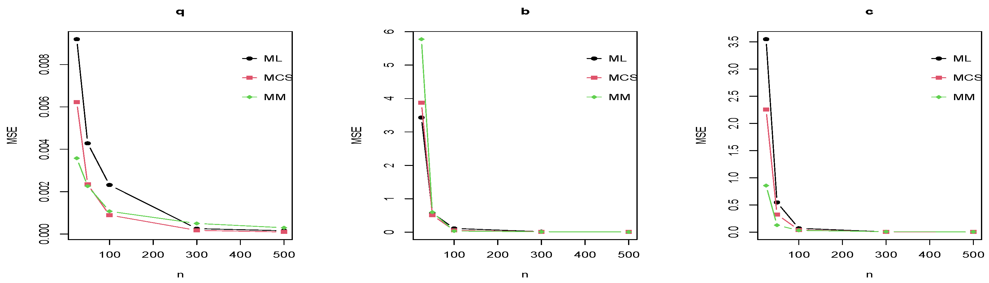
where ${\mathsf{\Lambda }}_{tr}=(q,b,c)$ represents the true vector of parameters, and $\widehat{\mathsf{\Lambda }}$ is the vector of estimates. The values of different estimates with the MSE and MAE are listed in Table 3, while the MSE for the three cases is presented in Figure 3, Figure 4 and Figure 5.

Table 3. Estimates, MSE, and MAE for ML, MCS, and MM methods across sample sizes under the three considered cases.

Case	n	Param	ML			MCS			MM
			Est.	MSE	MAE	Est.	MSE	MAE	Est.	MSE	MAE
I	25	q	0.3955	0.0398	0.0800	0.3256	0.0143	0.0625	0.3336	0.0142	0.0636
		b	5.0785	2.8537	0.5353	6.1032	5.3861	0.5765	5.7141	0.9435	0.3658
		c	2.0851	1.1948	0.9817	1.6543	0.4787	0.5320	1.4720	0.2135	0.3412
	50	q	0.3362	0.0106	0.0364	0.3040	0.0018	0.0312	0.3083	0.0024	0.0308
		b	5.4600	1.3511	0.4165	5.8819	0.1495	0.3037	5.7925	0.3609	0.2395
		c	1.7427	0.5042	0.6063	1.4912	0.2040	0.3833	1.3355	0.0688	0.2235
	100	q	0.3213	0.0052	0.0284	0.2958	0.0007	0.0217	0.2975	0.0008	0.0197
		b	5.5684	0.7951	0.3354	5.9862	0.1195	0.2935	5.9312	0.1131	0.2313
		c	1.5225	0.2956	0.3734	1.3635	0.1167	0.2459	1.2941	0.0555	0.1716
	300	q	0.3006	0.0012	0.0168	0.2916	0.0003	0.0138	0.2946	0.0002	0.0104
		b	5.8681	0.2735	0.2755	6.0351	0.0899	0.2540	5.9560	0.0743	0.2080
		c	1.2522	0.0444	0.0936	1.2227	0.0204	0.0802	1.2209	0.0156	0.0726
	500	q	0.2947	0.0003	0.0125	0.2911	0.0002	0.0120	0.2947	0.0001	0.0084
		b	5.9567	0.1060	0.2304	6.0337	0.0759	0.2376	5.9425	0.0594	0.1783
		c	1.2068	0.0083	0.0529	1.1993	0.0054	0.0516	1.2047	0.0063	0.0511
II	25	q	0.6800	0.0275	0.1082	0.6259	0.0227	0.0960	0.6507	0.0208	0.1070
		b	3.5083	7.4593	1.2938	3.9993	6.9559	1.1626	3.1571	1.4062	0.5632
		c	2.5023	1.6485	0.9655	2.1946	1.5941	0.7201	2.0138	0.8413	0.5751
	50	q	0.6469	0.0120	0.0713	0.6076	0.0073	0.05465	0.6013	0.0065	0.0571
		b	2.8721	1.3531	0.5648	3.1027	0.8159	0.3121	3.0665	0.2393	0.2507
		c	2.0039	0.5518	0.4657	1.8148	0.3561	0.3092	1.7165	0.1641	0.2494
	100	q	0.6117	0.0047	0.0460	0.5920	0.0022	0.0359	0.5950	0.0026	0.0368
		b	2.9011	0.1826	0.2592	3.0320	0.0822	0.1829	2.9970	0.0518	0.1602
		c	1.7207	0.1438	0.1938	1.6468	0.0568	0.1503	1.6348	0.0391	0.1419
	300	q	0.5925	0.0011	0.0238	0.5876	0.0006	0.0207	0.5934	0.0006	0.0181
		b	2.9876	0.0427	0.1445	3.0206	0.0251	0.1394	2.9730	0.0208	0.1169
		c	1.5979	0.0074	0.0671	1.5874	0.0069	0.0661	1.5976	0.0065	0.0636
	500	q	0.5904	0.0006	0.0183	0.5875	0.0005	0.0175	0.5944	0.0003	0.0134
		b	2.9931	0.0239	0.1214	3.0135	0.0213	0.1283	2.9578	0.0159	0.1028
		c	1.5884	0.0043	0.0523	1.5822	0.0043	0.0517	1.5950	0.0036	0.0462
III	25	q	0.8063	0.0091	0.0775	0.8058	0.0062	0.0415	0.8040	0.0035	0.0426
		b	2.3093	3.4312	0.9341	2.2286	3.8768	0.7902	2.2847	5.7755	0.8821
		c	3.0511	3.5497	1.0144	2.7986	2.2571	0.6704	2.4652	0.8559	0.4612
	50	q	0.7917	0.0042	0.0478	0.7927	0.0023	0.0313	0.7914	0.0022	0.0321
		b	1.8028	0.5761	0.3421	1.7772	0.5096	0.2749	1.7676	0.5987	0.2765
		c	2.3911	0.5459	0.3773	2.2840	0.3245	0.2761	2.1883	0.1271	0.2031
	100	q	0.7923	0.0023	0.0261	0.7947	0.0008	0.0183	0.7944	0.0010	0.0230
		b	1.6809	0.1120	0.1766	1.6619	0.0530	0.1576	1.6550	0.0352	0.1366
		c	2.1721	0.0696	0.1404	2.1467	0.0403	0.1229	2.1301	0.0310	0.1212
	300	q	0.7991	0.0002	0.0115	0.7962	0.0001	0.0089	0.7949	0.0004	0.0147
		b	1.6181	0.0155	0.0951	1.6319	0.0127	0.0859	1.6355	0.0111	0.0757
		c	2.1101	0.0045	0.0466	2.0994	0.0051	0.0536	2.0954	0.0078	0.0642
	500	q	0.7988	0.0001	0.0094	0.7962	$9.3\times {10}^{-5}$	0.0075	0.7960	0.0002	0.0114
		b	1.6147	0.0106	0.0807	1.6272	0.0082	0.0693	1.6256	0.0060	0.0567
		c	2.1033	0.0018	0.0321	2.0938	0.0027	0.0410	2.0939	0.0046	0.0509

Figure 3. Plot of the MSE of the estimates of the parameters q, b and c, respectively, for the DEGWR distribution for Case I.

Figure 4. Plot of the MSE of the estimates of the parameters q, b and c, respectively, for the DEGWR distribution for Case II.

Figure 5. Plot of the MSE of the estimates of the parameters q, b and c, respectively, for the DEGWR distribution for Case III.

According to Table 3 and Figure 3, Figure 4 and Figure 5, the simulation results show a noticeable improvement in the parameters’ estimates: the MSE and the MAE decrease when the sample size increases. This proves the consistency of all estimates in the three approaches. For parameter q, the three methods ML, MCS, and MM exhibit similar behavior with an advantage to the MCS in small samples while the MM becomes comparable or superior in moderate and large samples. For parameter b, the results indicates that the MM attained the lowest MSE in most scenarios followed by the MCS, while the performance of ML improved for large samples. For parameter c, the MM displays a marked superiority in terms of MSE compared to ML and MCS in most cases especially for small and moderate sample sizes. Although the behavior of the MCS is enhanced by increasing the sample size, it rarely exceeds those obtained by the MM.

7. Application

In this section, four datasets from medicine and education are analyzed to assess the performance of the DEGWR distribution. For comparison, the discrete exponential odd Weibull exponential (DEOWE) by [42], the DEMOR explained in [34], the DNGR proposed by [35], the discrete Weibull exponential (DWE) introduced by [10], the discrete Burr (DBurr) by [43], the discrete Fréchet (DFr) provided by [44], and the DR by [30] are acquired to test the ability of the DEGWR distribution to model medical and educational data. To compare the performance of the distributions’ fitting, some evaluation metrics are considered: the Akaike information criterion (AIC), the Bayesian information criterion (BIC),the Hannan–Quinn information criterion (HQIC), and the p-value of the Kolmogorov–Smirnov test. These criteria are selected because they provide different degrees of penalization for the model complexity and capture various aspects of the model selection. Therefore, using these criteria together, rather than relying on a single criterion, enables a robust and comprehensive assessment of the distributions in modeling real data. The data description and the results are listed below.

7.1. Dataset 1

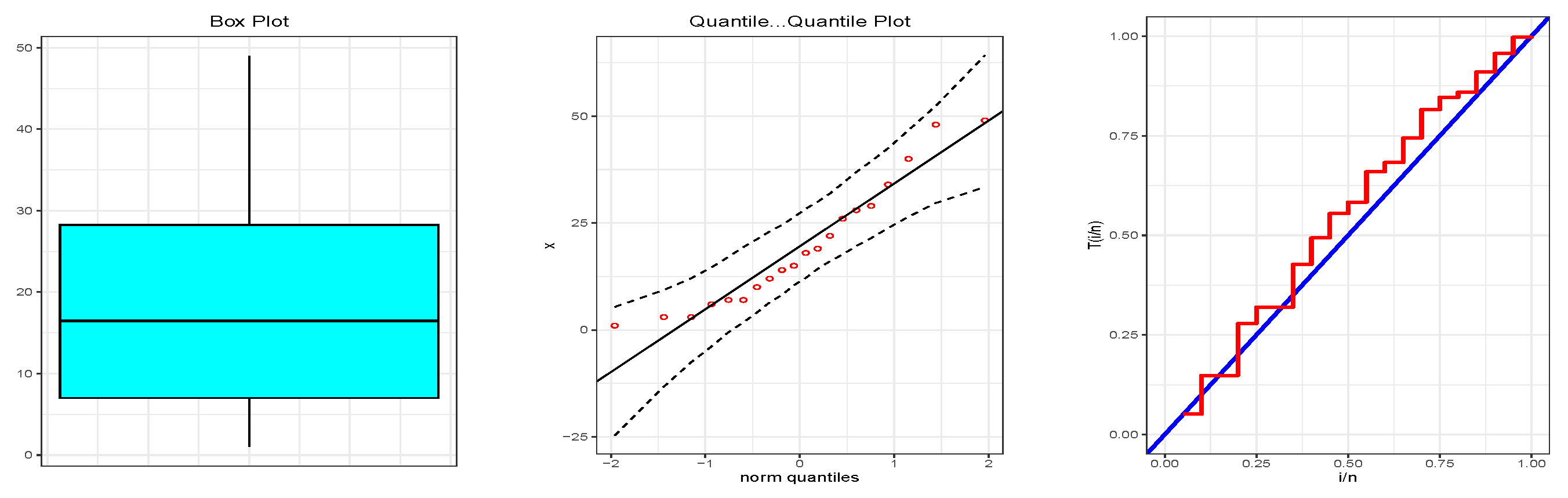
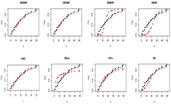
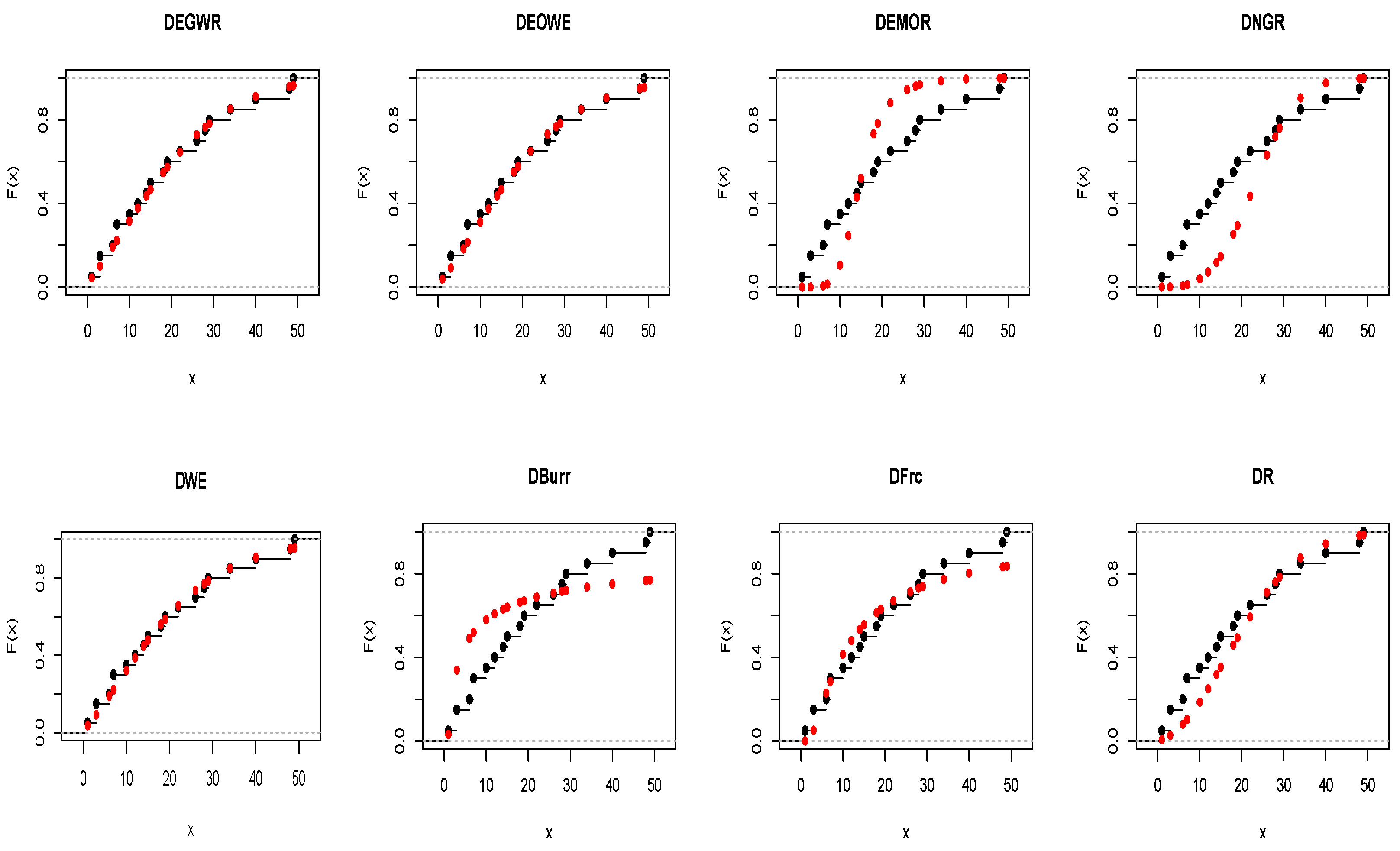
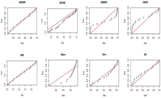
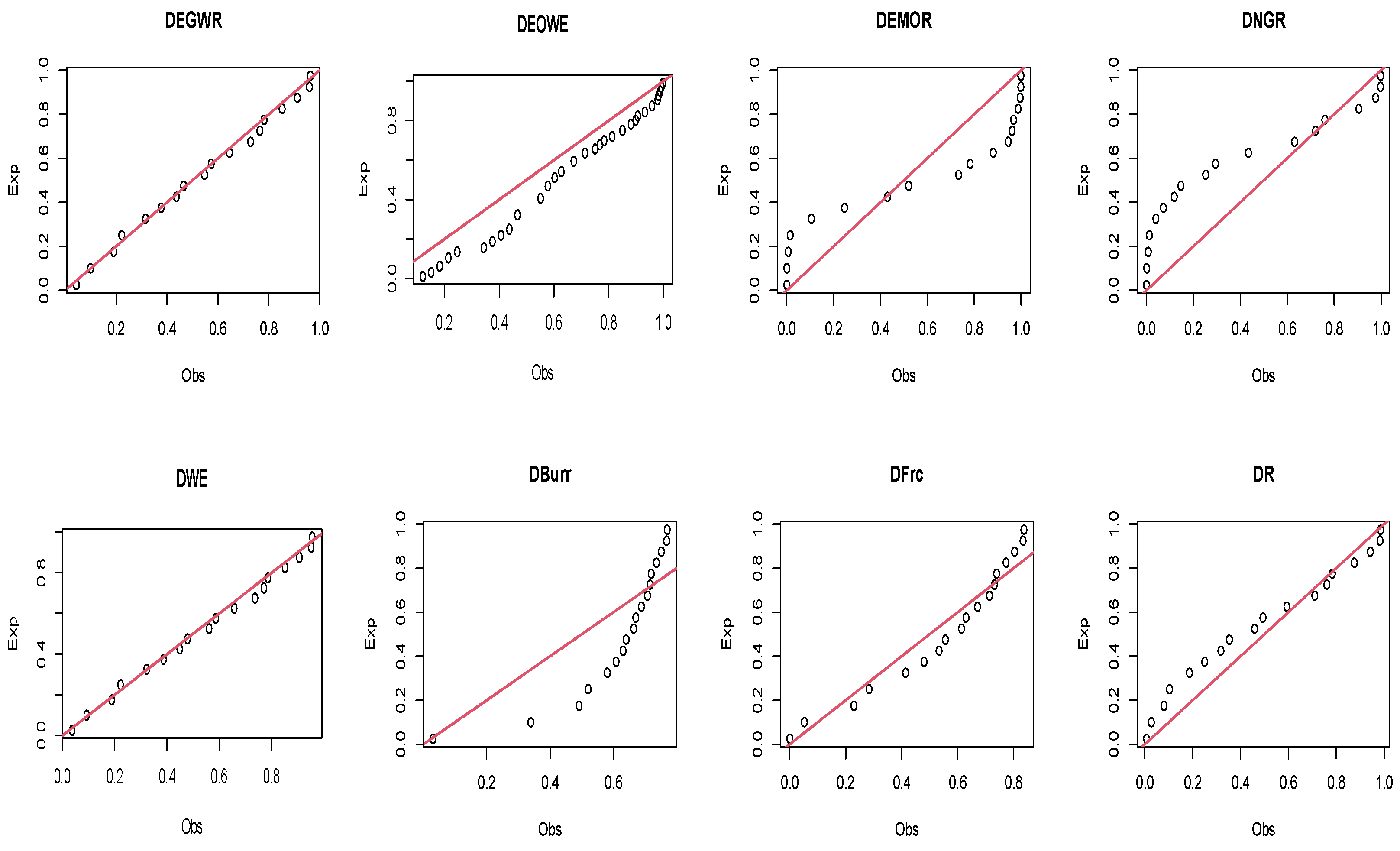
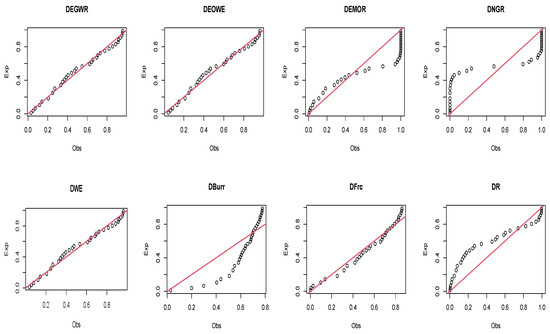
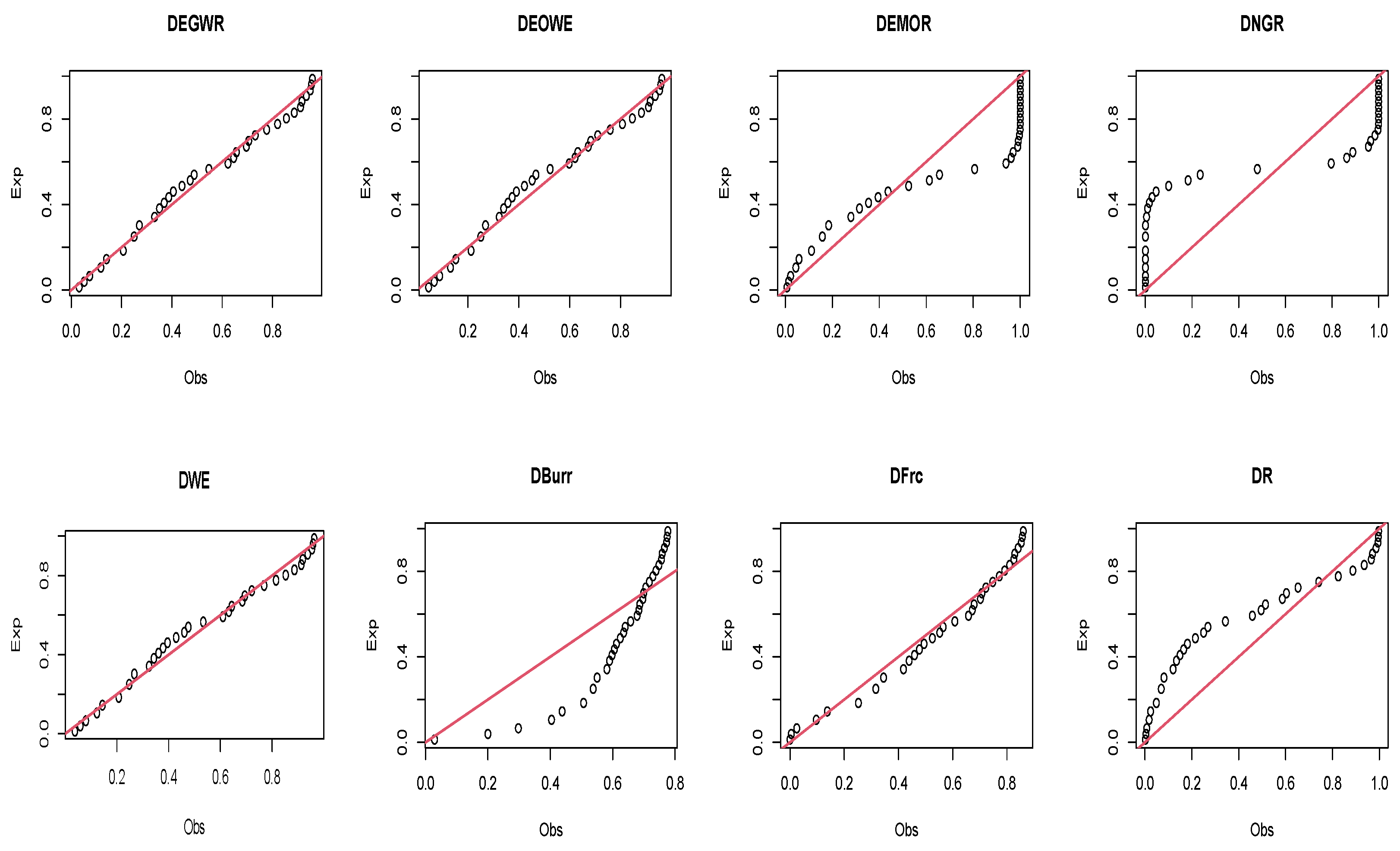
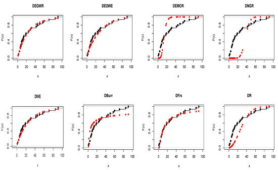
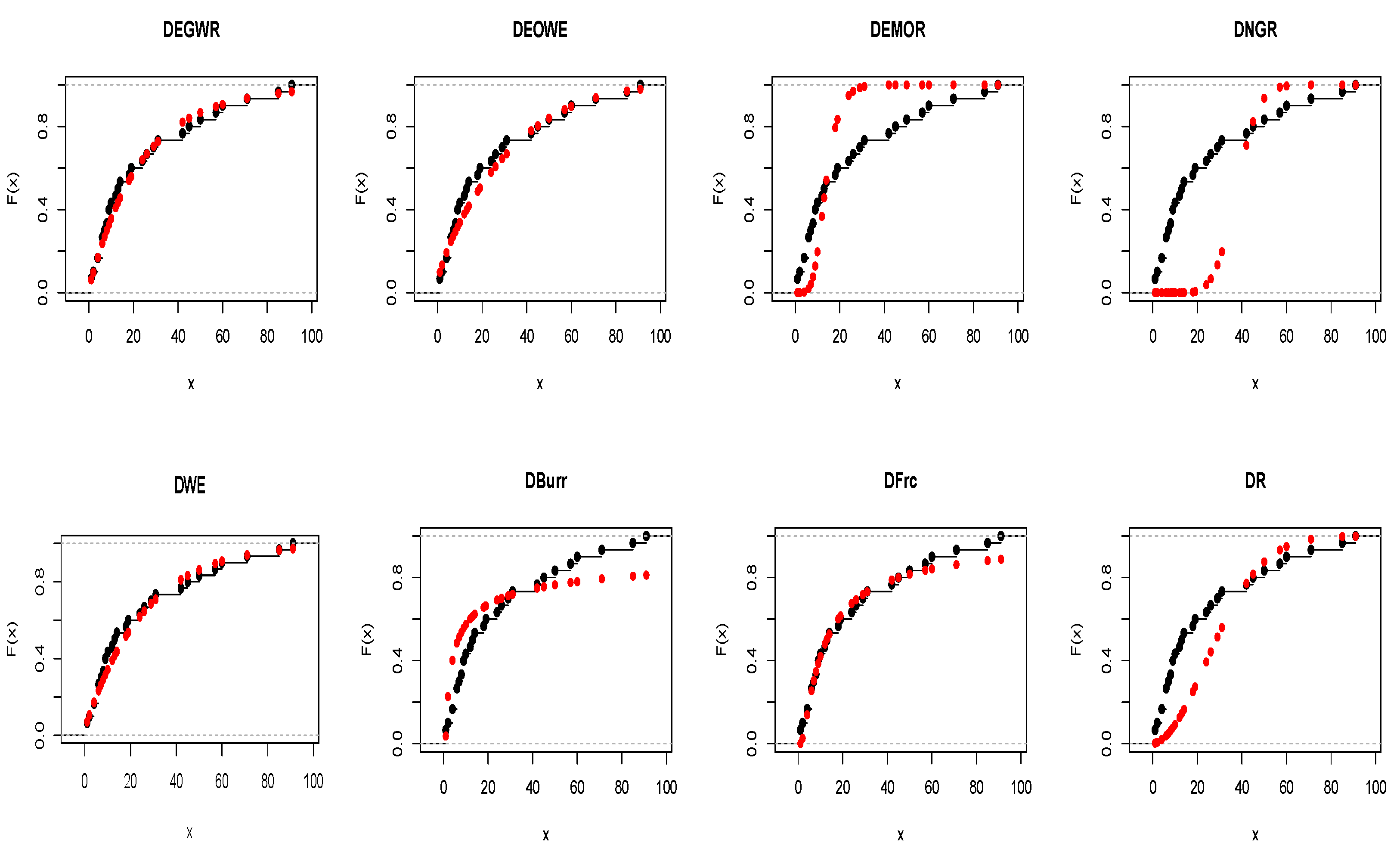
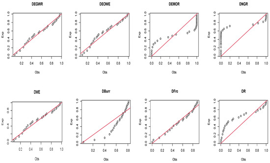
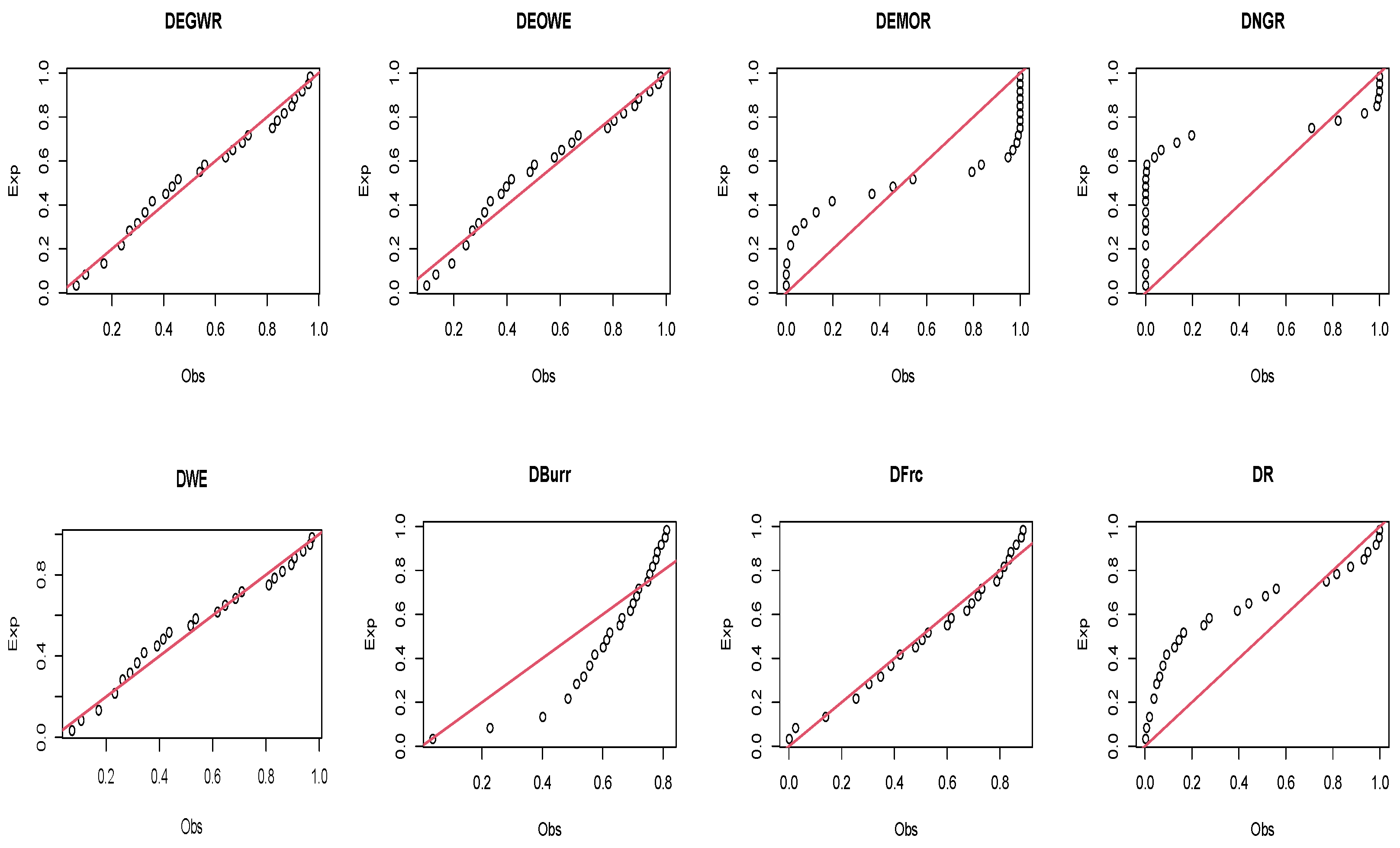
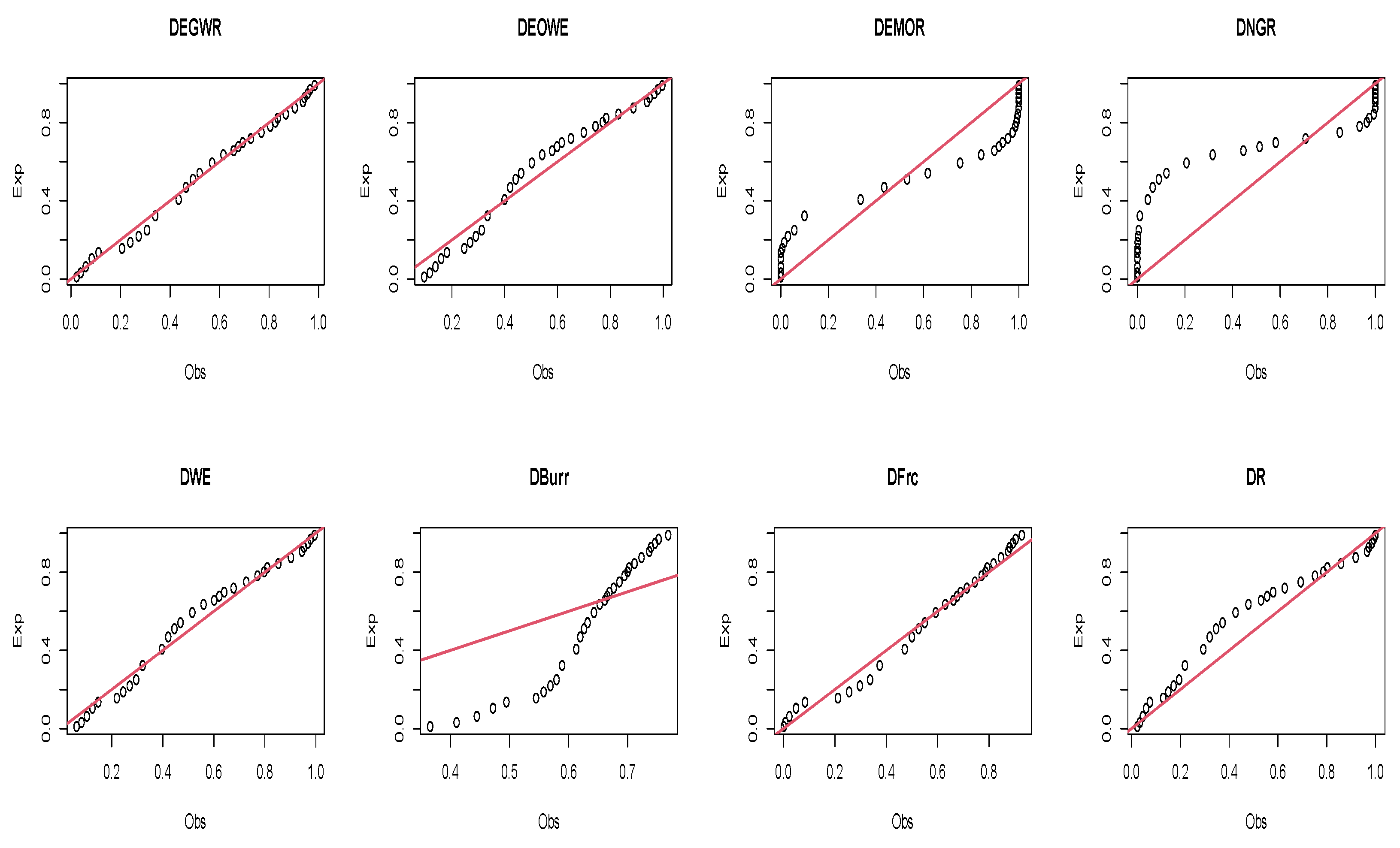
The data were used in [45] and represent the remission time (in weeks) for 20 patients who suffer from leukemia and were exposed to a particular treatment, as follows: 1, 3, 3, 6, 7, 7, 10, 12, 14, 15, 18, 19, 22, 26, 28, 29, 34, 40, 48, and 49. Figure 6 presents the boxplot together with the Q-Q plot and TTT plot for the remission time. Moreover, Table 4 displays the MLE of the parameters, as well as the goodness-of fit measures. The pp-plot and the theoretical and empirical CDF for all distributions are presented in Figure 7 and Figure 8, respectively.

Figure 6. The boxplot, Q-Q plot, and TTT plot for Dataset 1.

Table 4. Maximum likelihood estimates and goodness-of-fit measures for Dataset 1.

Model	MLEs	AIC	BIC	HQIC	p-Value
DEGWR	$\widehat{q}=0.997,\widehat{b}=0.677,\widehat{c}=0.883$	162.999	165.986	163.582	0.9993
DEOWE	$\widehat{a}=1.253,\widehat{b}=0.530,\widehat{\lambda }=0.036$	163.433	166.419	164.016	0.9985
DEMOR	$\widehat{q}=0.998,\widehat{\theta }=0.059,\widehat{\alpha }=3.621$	230.3267	233.314	230.909	0.0713
DNGR	$\widehat{\alpha }=1.6931,\widehat{\beta }=2.0991,\widehat{\theta }=0.0033$	204.8076	207.7948	205.3908	0.0151
DWE	$\widehat{\alpha }=1.3730,\widehat{b}=0.6216,\widehat{\theta }=0.0284$	163.2237	166.2109	163.8068	0.9983
DBurr	$\widehat{q}=0.956,\widehat{\alpha }=8.448$	189.462	191.453	189.851	0.0192
DFr	$\widehat{\alpha }=1.005,\widehat{\beta }=8.821$	170.233	172.225	170.622	0.6600
DR	$\widehat{q}=0.998$	164.350	165.346	164.544	0.4001

Figure 7. Theoretical and empirical CDF of the DEGWR and competing distributions for Dataset 1.

Figure 8. The pp-plot of the DEGWR and competing distributions for Dataset 1.

Figure 6 suggests a slight skewness and an increasing hazard rate in the remission time data. This results in an increased risk of relapse as the remission duration increases.

7.2. Dataset 2

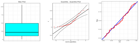
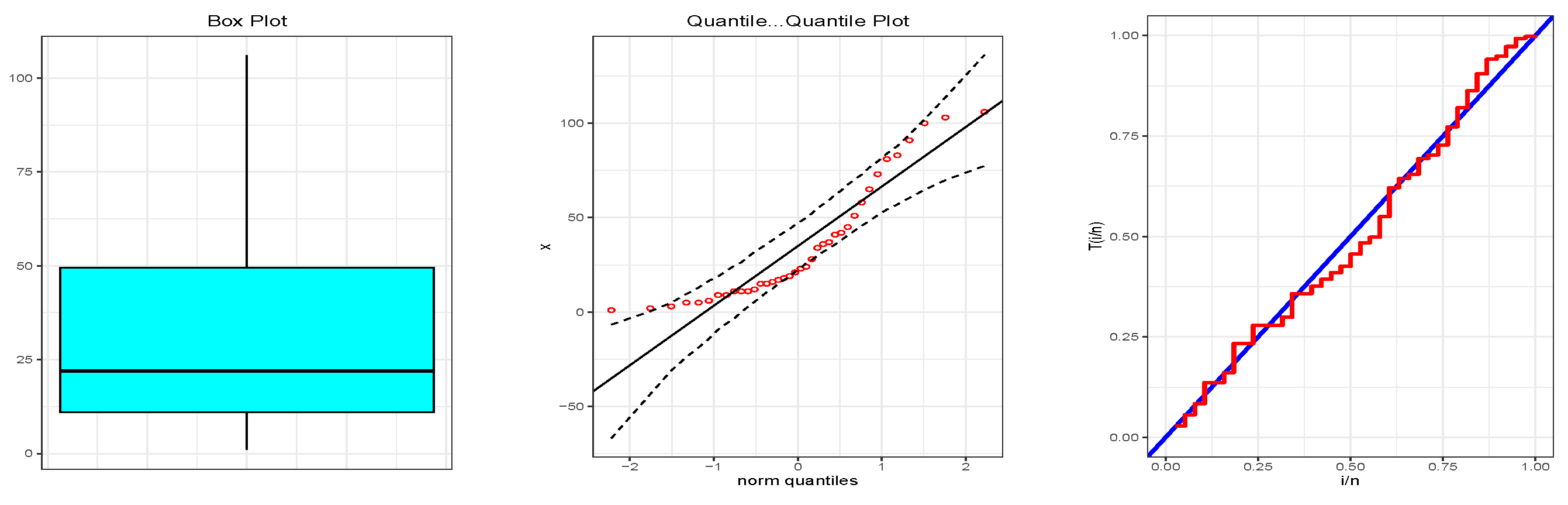
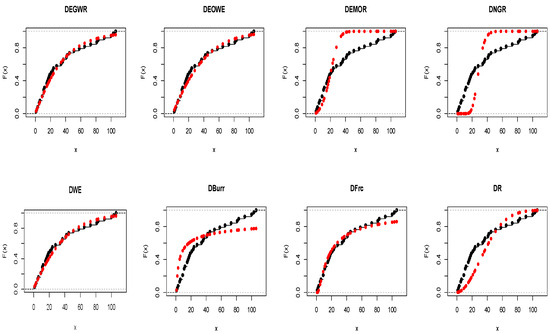
The second dataset was discussed in [21] and represents the daily number of deaths caused by COVID-19 in Punjab between 24 March 2020 and 30 April 2020. The data are: 1, 2, 3, 5, 5, 6, 9, 9, 11, 11, 11, 12, 15, 15, 16, 17, 18, 19, 21, 23, 24, 28, 34, 36, 37, 41, 42, 45, 51, 58, 65, 73, 81, 83, 91, 100, 103, and 106. The boxplot, Q-Q plot, and TTT plot for the data are presented in Figure 9. Additionally, the MLEs with the goodness-of-fit measures are shown in Table 5, and the theoretical and empirical CDF and the pp-plot are shown in Figure 10 and Figure 11, respectively.

Figure 9. The boxplot, Q-Q plot, and TTT plot for Dataset 2.

Table 5. Maximum likelihood estimates and goodness-of-fit measures for Dataset 2.

Model	MLEs	AIC	BIC	HQIC	p-Value
DEGWR	$\widehat{q}=0.954,\widehat{b}=1.401,\widehat{c}=0.462$	352.303	357.216	354.051	0.9912
DEOWE	$\widehat{a}=0.995,\widehat{b}=0.596,\widehat{\lambda }=0.023$	352.816	357.728	354.564	0.9530
DEMOR	$\widehat{q}=0.997,\widehat{\theta }=4.669,\widehat{\alpha }=0.785$	679.276	684.188	681.024	$1.17\times {10}^{-4}$
DNGR	$\widehat{\alpha }=21.3664,\widehat{\beta }=8.4819,\widehat{\theta }=0.0030$	953.2682	958.1809	955.0161	$2.233\times {10}^{-6}$
DWE	$\widehat{\alpha }=1.1181,\widehat{b}=0.4522,\widehat{\theta }=0.0122$	352.3898	357.3026	354.1377	0.9749
DBurr	$\widehat{q}=0.9580,\widehat{\alpha }=7.569$	401.742	405.017	402.907	$1.94\times {10}^{-4}$
DFr	$\widehat{\alpha }=0.897,\widehat{\beta }=12.859$	362.229	365.504	363.395	0.4465
DR	$\widehat{q}=0.999$	375.400	377.037	375.982	0.0014

Figure 10. Theoretical and empirical CDF of the DEGWR and competing distributions for Dataset 2.

Figure 11. The pp-plot of the DEGWR and competing distributions for Dataset 2.

Figure 9 shows that the daily number of deaths deviated from normality, with a bathtub-shaped hazard.

7.3. Dataset 3

The third dataset was related to the period of symptom relief (in weeks) for 30 patients diagnosed with leukemia who received the same treatment. This is mentioned in [46] as follows: 1, 1, 2, 4, 4, 6, 6, 6, 7, 8, 9, 9, 10, 12, 13, 14, 18, 19, 24, 26, 29, 31, 42, 45, 50, 57, 60, 71, 85, and 91. The boxplot, Q-Q plot, and TTT plot for the period of symptom relief are displayed in Figure 12. Furthermore, the MLEs for all distributions are listed in Table 6, and the theoretical and empirical CDF, as well as the pp-plot are displayed in Figure 13 and Figure 14, respectively.

Figure 12. The boxplot, Q-Q plot, and TTT plot for Dataset 3.

Table 6. The MLEs and goodness-of-fit measures for different distributions for Dataset 3.

Model	MLEs	AIC	BIC	HQIC	p-Value
DEGWR	$\widehat{q}=0.881,\widehat{b}=1.695,\widehat{c}=0.379$	260.463	264.667	261.817	0.9635
DEOWE	$\widehat{a}=0.778,\widehat{b}=0.230,\widehat{\lambda }=0.027$	262.313	266.517	263.658	0.8161
DEMOR	$\widehat{q}=0.995,\widehat{\theta }=0.257,\widehat{\alpha }=3.330$	543.458	547.661	544.803	0.0016
DENGR	$\widehat{\alpha }=1.4116,\widehat{\beta }=7.8703,\widehat{\theta }=0.0024$	812.0068	816.2104	813.3516	$1.27\times {10}^{-9}$
DWE	$\widehat{\alpha }=1.0119,\widehat{b}=0.7462,\widehat{\theta }=0.0287$	261.0892	265.2928	262.4339	0.9419
DBurr	$\widehat{q}=0.947,\widehat{\alpha }=6.839$	286.589	289.391	287.487	0.0046
DFr	$\widehat{\alpha }=0.899,\widehat{\beta }=8.506$	264.291	267.094	265.188	0.8466
DR	$\widehat{q}=0.999$	288.484	289.885	288.933	$4.31\times {10}^{-4}$

Figure 13. Theoretical and empirical CDF of the DEGWR and competing distributions for Dataset 3.

Figure 14. The pp-plot of the DEGWR and competing distributions for Dataset 3.

Figure 12 indicates a noticeable departure from normality, specifically right skewness, in the period of symptom relief with a decrease to approximately constant hazard behavior.

7.4. Dataset 4

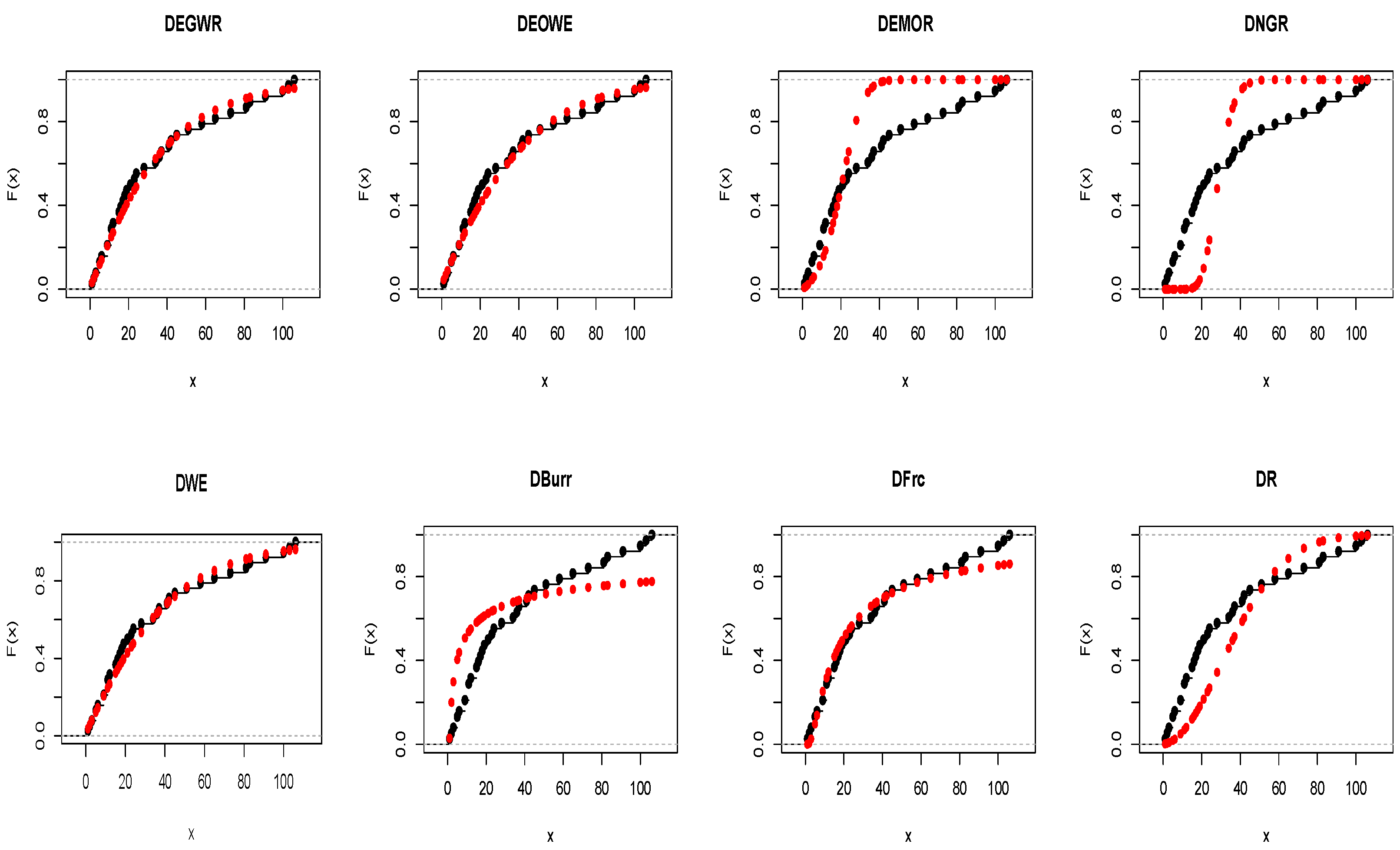
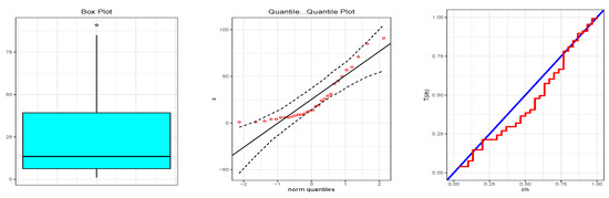
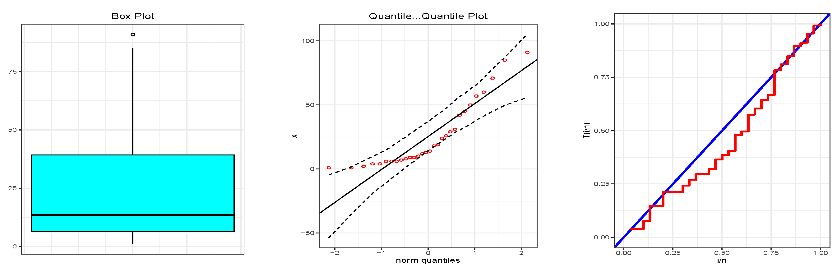
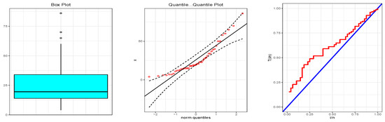
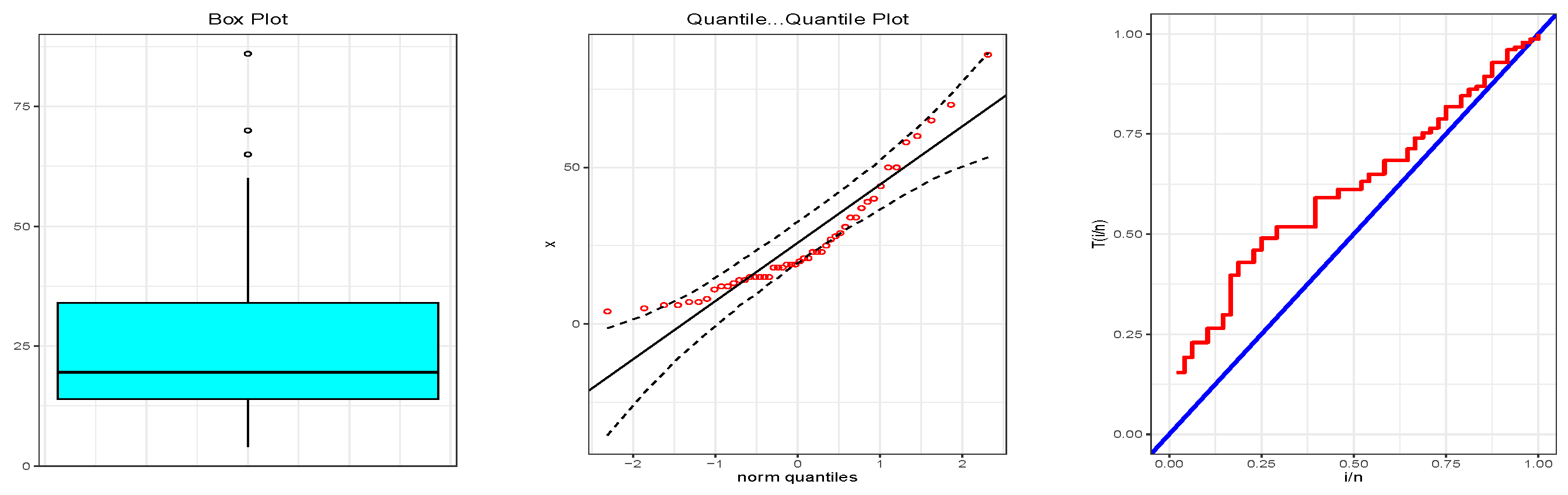
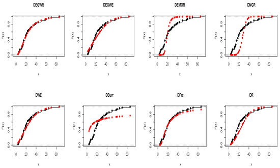
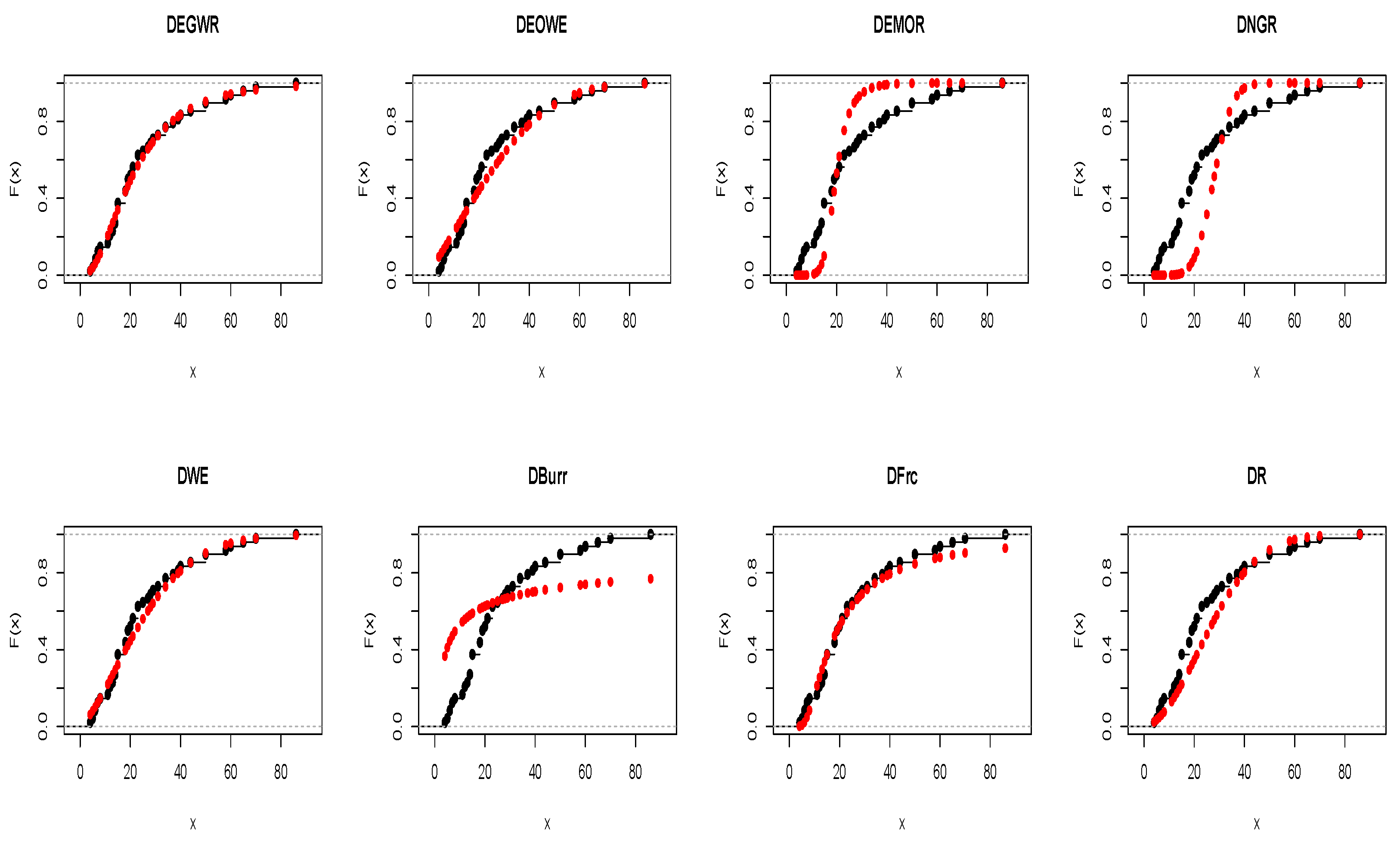
The last dataset represents the marks of 48 Indian students in mathematics who enrolled in the slow-paced program at the Institute of Technology at Kanpur. The data were collected in 2003 and mentioned in [47]. The students’ marks are as follows: 29, 25, 50, 15, 13, 27, 15, 18, 7, 7, 8, 19, 12, 18, 5, 21, 15, 86, 21, 15, 14, 39, 15, 14, 70, 44, 6, 23, 58, 19, 50, 23, 11, 6, 34, 18, 28, 34, 12, 37, 4, 60, 20, 23, 40, 65, 19, and 31. Figure 15 shows the boxplot, Q-Q plot, and TTT plot for students’ marks. In addition, the MLEs for all distributions are presented in Table 7. Figure 16 and Figure 17 display the theoretical and empirical CDF, as well as the pp-plot, respectively.

Figure 15. The boxplot, Q-Q plot, and TTT plot for Dataset 4.

Table 7. The MLEs and goodness-of-fit measures of different distributions for Dataset 4.

Model	MLEs	AIC	BIC	HQIC	KS	p-Value
DEGWR	$\widehat{q}=0.7059,\widehat{b}=8.0528,\widehat{c}=0.3220$	398.9836	404.5972	401.1050	0.0780	0.9323
DEOWE	$\widehat{a}=1.0971,\widehat{b}=0.1065,\widehat{\lambda }=0.0232$	407.9399	413.5535	410.0613	0.1223	0.4694
DEMOR	$\widehat{q}=0.9979,\widehat{\theta }=0.0415,\widehat{\alpha }=6.0981$	576.4608	582.0744	578.5822	0.2753	0.0014
DENGR	$\widehat{\alpha }=1.4560,\widehat{\beta }=7.8467,\widehat{\theta }=0.00407$	711.5970	717.2106	713.7184	0.4401	$1.68\times {10}^{-8}$
DWE	$\widehat{\alpha }=1.5459,\widehat{b}=0.0926,\widehat{\theta }=0.0031$	403.2172	408.8308	405.3386	0.1093	0.6148
DBurr	$\widehat{q}=0.9190,\widehat{\alpha }=3.8861$	498.9836	502.7260	500.3979	0.4032	$3.33\times {10}^{-7}$
DFr	$\widehat{\alpha }=1.4731,\widehat{\beta }=14.8168$	404.5561	408.2985	405.9704	0.1080	0.6299
DR	$\widehat{q}=0.9990$	405.7879	407.6591	406.4950	0.1986	0.0453

Figure 16. Theoretical and empirical CDF of the DEGWR and competing distributions for Dataset 4.

Figure 17. The pp-plot of the DEGWR and competing distributions for Dataset 4.

Figure 15 illustrates that the grade distribution is clearly not well approximated by a normal distribution with an increasing, and approximately constant, hazard rate function.

8. Conclusions

Introducing new statistical distributions capable of fitting data on a discrete scale is of considerable importance. In this study, a discretized version of the EGW-G family was constructed using the survival discretization method to extend the family’s flexibility for modeling count and discrete data. This approach enabled the construction of a new adaptable discrete distribution, named the DEGWR distribution, as a member of this family. This distribution is highly adaptable, as it can model discrete data with various symmetric and asymmetric forms. Some statistical properties for the DEGWR distribution, including moments, the moment-generating function, entropy, and order statistics, are studied. The distribution parameters are estimated using three classical methods, ML, MCS, and MM. Moreover, the precision of the three methods’ estimators is evaluated in three simulation scenarios. Furthermore, the DEGWR distribution is employed to analyze four datasets. The empirical results demonstrate the superior flexibility of DEGWR in fitting the examined datasets compared with the considered distributions, as it yielded the lowest values for various model selection criteria.

References

- Chakraborty, S. Generating discrete analogues of continuous probability distributions—A survey of methods and constructions. J. Stat. Distrib. Appl. 2015, 2, 6. [Google Scholar] [CrossRef] [Scilit]
- Kemp, A.W. Classes of discrete lifetime distributions. Commun. Stat. Theory Methods 2004, 33, 3069–3093. [Google Scholar] [CrossRef] [Scilit]
- Para, B.; Jan, T. On discrete three-parameter Burr type XII and discrete Lomax distributions and their applications to model count data from medical science. Biom. Biostat. Int. J. 2016, 4, 1–15. [Google Scholar]
- Eliwa, M.; Alhussain, Z.A.; El-Morshedy, M. Discrete Gompertz-G family of distributions for over-and under-dispersed data with properties, estimation, and applications. Mathematics 2020, 8, 358. [Google Scholar] [CrossRef] [Scilit]
- Almetwally, E.M.; Abdo, D.A.; Hafez, E.; Jawa, T.M.; Sayed-Ahmed, N.; Almongy, H.M. The new discrete distribution with application to COVID-19 Data. Results Phys. 2022, 32, 104987. [Google Scholar] [CrossRef] [Scilit]
- Pandey, A.; Singh, R.P.; Tyagi, A. An inferential study of discrete Burr-Hatke exponential distribution under complete and censored data. Reliab. Theory Appl. 2022, 17, 109–122. [Google Scholar]
- Eledum, H.; El-Alosey, A. Discrete Kumaraswamy Erlang-truncated exponential distribution with applications to count data. J. Stat. Appl. Probab. 2023, 12, 725–739. [Google Scholar] [CrossRef] [Scilit]
- Ahsan-ul Haq, M.; Hussain, M.N.; Babar, A.; Al-Essa, L.A.; Eliwa, M.S. Analysis, Estimation, and Practical Implementations of the Discrete Power Quasi-Xgamma Distribution. J. Math. 2024, 2024, 1913285. [Google Scholar] [CrossRef] [Scilit]
- Maya, R.; Jodrá, P.; Aswathy, S.; Irshad, M. The discrete new XLindley distribution and the associated autoregressive process. Int. J. Data Sci. Anal. 2025, 20, 1767–1793. [Google Scholar] [CrossRef] [Scilit]
- Balubaid, A.; Klakattawi, H.; Alsulami, D. On the Discretization of the Weibull-G Family of Distributions: Properties, Parameter Estimates, and Applications of a New Discrete Distribution. Symmetry 2024, 16, 1519. [Google Scholar] [CrossRef] [Scilit]
- Cordeiro, G.M.; Ortega, E.M.; da Cunha, D.C. The exponentiated generalized class of distributions. J. Data Sci. 2013, 11, 1–27. [Google Scholar] [CrossRef] [Scilit]
- Alzaatreh, A.; Lee, C.; Famoye, F. A new method for generating families of continuous distributions. Metron 2013, 71, 63–79. [Google Scholar] [CrossRef] [Scilit]
- Alzaatreh, A.; Famoye, F.; Lee, C. Weibull-Pareto distribution and its applications. Commun. Stat. Theory Methods 2013, 42, 1673–1691. [Google Scholar] [CrossRef] [Scilit]
- Alzaatreh, A.; Ghosh, I. On the Weibull-X family of distributions. J. Stat. Theory Appl. 2015, 14, 169–183. [Google Scholar] [CrossRef] [Scilit]
- Alsulami, D. A new extension of the Rayleigh distribution: Properties, different methods of estimation, and an application to medical data. AIMS Math. 2025, 10, 7636–7663. [Google Scholar] [CrossRef] [Scilit]
- Klakattawi, H.S. A Novel Exponentiated Generalized Weibull Exponential Distribution: Properties, Estimation, and Regression Model. Axioms 2025, 14, 706. [Google Scholar] [CrossRef] [Scilit]
- Eugene, N.; Lee, C.; Famoye, F. Beta-normal distribution and its applications. Commun. Stat. Theory Methods 2002, 31, 497–512. [Google Scholar] [CrossRef] [Scilit]
- Cordeiro, G.M.; De Castro, M. A new family of generalized distributions. J. Stat. Comput. Simul. 2011, 81, 883–898. [Google Scholar] [CrossRef] [Scilit]
- Mahdavi, A.; Kundu, D. A new method for generating distributions with an application to exponential distribution. Commun. Stat. Theory Methods 2017, 46, 6543–6557. [Google Scholar] [CrossRef] [Scilit]
- Ibrahim, M.; Ali, M.M.; Yousof, H.M. The discrete analogue of the Weibull G family: Properties, different applications, Bayesian and non-Bayesian estimation methods. Ann. Data Sci. 2023, 10, 1069–1106. [Google Scholar] [CrossRef] [Scilit]
- El-Morshedy, M.; Shahen, H.S.; Almohaimeed, B.; Eliwa, M.S. Discrete Single-Factor Extension of the Exponential Distribution: Features and Modeling. Axioms 2022, 11, 737. [Google Scholar] [CrossRef] [Scilit]
- Eliwa, M.S.; El-Morshedy, M.; Yousof, H.M. A discrete exponential generalized-G family of distributions: Properties with Bayesian and non-Bayesian estimators to model medical, engineering and agriculture data. Mathematics 2022, 10, 3348. [Google Scholar] [CrossRef] [Scilit]
- Balubaid, A.; Alsulami, D. Discretization of the Alpha Power Weibull-G Family of Distributions: A Novel Discrete Distribution with Properties, Estimation, and Applications to Medical and Educational Data. Int. J. Anal. Appl. 2025, 23, 239. [Google Scholar] [CrossRef] [Scilit]
- Rayleigh, J.W.S.B. The Theory of Sound; Macmillan: New York, NY, USA, 1896; Volume 2. [Google Scholar]
- Almongy, H.M.; Almetwally, E.M.; Aljohani, H.M.; Alghamdi, A.S.; Hafez, E. A new extended Rayleigh distribution with applications of COVID-19 data. Results Phys. 2021, 23, 104012. [Google Scholar] [CrossRef] [Scilit]
- Kilai, M.; Waititu, G.A.; Kibira, W.A.; Abd El-Raouf, M.; Abushal, T.A. A new versatile modification of the Rayleigh distribution for modeling COVID-19 mortality rates. Results Phys. 2022, 35, 105260. [Google Scholar] [CrossRef] [Scilit]
- Bhat, A.; Ahmad, S.P.; Almetwally, E.M.; Yehia, N.; Alsadat, N.; Tolba, A.H. The odd lindley power rayleigh distribution: Properties, classical and bayesian estimation with applications. Sci. Afr. 2023, 20, e01736. [Google Scholar] [CrossRef] [Scilit]
- Obi, C.D.; Chukwuma, P.O.; Igbokwe, C.P.; Ibeakuzie, P.O.; Anabike, I.C. A Novel Extension of Rayleigh Distribution: Characterization, Estimation, Simulations and Applications. J. Xidian Univ. 2024, 18, 177–188. [Google Scholar]
- Abdulrahman, A.T.; Rashedi, K.A.; Alshammari, T.S.; Hussam, E.; Alharthi, A.S.; Albayyat, R.H. A new extension of the Rayleigh distribution: Methodology, classical, and Bayes estimation, with application to industrial data. AIMS Math 2025, 10, 3710–3733. [Google Scholar] [CrossRef] [Scilit]
- Roy, D. Discrete rayleigh distribution. IEEE Trans. Reliab. 2004, 53, 255–260. [Google Scholar] [CrossRef] [Scilit]
- Hussain, T.; Ahmad, M. Discrete inverse rayleigh distribution. Pak. J. Stat. 2014, 30, 203–222. [Google Scholar]
- Shahid, N.; Rahee, R. Discrete modified inverse rayleigh distribution. Pak. J. Stat. 2019, 35, 75–95. [Google Scholar]
- Ma, H.J.; Yan, Z.Z. Discrete Weibull-Rayleigh distribution properties and parameter estimations. Therm. Sci. 2022, 26, 2627–2636. [Google Scholar] [CrossRef] [Scilit]
- Jayakumar, K.; Sankaran, K. A generalization of discrete Weibull distribution. Commun. Stat. Theory Methods 2018, 47, 6064–6078. [Google Scholar] [CrossRef] [Scilit]
- Haj Ahmad, H.; Ramadan, D.A.; Almetwally, E.M. Evaluating the discrete generalized Rayleigh distribution: Statistical inferences and applications to real data analysis. Mathematics 2024, 12, 183. [Google Scholar] [CrossRef] [Scilit]
- Rényi, A. On measures of entropy and information. In Proceedings of the Fourth Berkeley Symposium on Mathematical Statistics and Probability, Volume 1: Contributions to the Theory of Statistics; University of California Press: Oakland, CA, USA, 1961; Volume 4, pp. 547–562. [Google Scholar]
- Shannon, C.E. A mathematical theory of communication. Bell Syst. Tech. J. 1948, 27, 379–423. [Google Scholar] [CrossRef] [Scilit]
- Arnold, B.C.; Balakrishnan, N.; Nagaraja, H.N. A First Course in Order Statistics; Wiley: Hoboken, NJ, USA, 1992. [Google Scholar]
- Berkson, J. Minimum chi-square, not maximum likelihood! Ann. Stat. 1980, 8, 457–487. [Google Scholar] [CrossRef] [Scilit]
- Harris, R.; Kanji, G. On the use of minimum chi-square estimation. J. R. Stat. Soc. Ser. D Stat. 1983, 32, 379–394. [Google Scholar] [CrossRef] [Scilit]
- Khan, M.A.; Khalique, A.; Abouammoh, A. On estimating parameters in a discrete Weibull distribution. IEEE Trans. Reliab. 1989, 38, 348–350. [Google Scholar] [CrossRef] [Scilit]
- Nagy, M.; Almetwally, E.M.; Gemeay, A.M.; Mohammed, H.S.; Jawa, T.M.; Sayed-Ahmed, N.; Muse, A.H. The New Novel Discrete Distribution with Application on COVID-19 Mortality Numbers in Kingdom of Saudi Arabia and Latvia. Complexity 2021, 2021, 7192833. [Google Scholar] [CrossRef] [Scilit]
- Krishna, H.; Pundir, P.S. Discrete Burr and discrete Pareto distributions. Stat. Methodol. 2009, 6, 177–188. [Google Scholar] [CrossRef] [Scilit]
- Nadarajah, S.; Lyu, J. New discrete heavy tailed distributions as models for insurance data. PLoS ONE 2023, 18, e0285183. [Google Scholar] [CrossRef] [Scilit] [PubMed]
- Bakouch, H.S.; Jazi, M.A.; Nadarajah, S. A new discrete distribution. Statistics 2014, 48, 200–240. [Google Scholar] [CrossRef] [Scilit]
- Lawless, J.F. Statistical Models and Methods for Lifetime Data; John Wiley & Sons: Hoboken, NJ, USA, 2011. [Google Scholar]
- Gupta, R.D.; Kundu, D. A new class of weighted exponential distributions. Statistics 2009, 43, 621–634. [Google Scholar] [CrossRef] [Scilit]
Disclaimer/Publisher’s Note: The statements, opinions and data contained in all publications are solely those of the individual author(s) and contributor(s) and not of MDPI and/or the editor(s). MDPI and/or the editor(s) disclaim responsibility for any injury to people or property resulting from any ideas, methods, instructions or products referred to in the content. |
© 2026 by the author. Licensee MDPI, Basel, Switzerland. This article is an open access article distributed under the terms and conditions of the Creative Commons Attribution (CC BY) license.