Spectrally Negative Lévy Risk Model Under Multi-Layer Ratcheting Dividend Strategy and Capital Injections

Abstract

In this study, we investigate the mixed n-layer ratcheting dividend and capital injection policies for a spectrally negative Lévy risk model, where dividend distributions are implemented continuously in a non-decreasing manner, and capital injections are conducted discretely at the jump instants of an independent Poisson process. We incorporate both terminal values and transaction costs into the analysis, making the model more in line with practical scenarios. The value function and the Laplace transform of the ruin time are derived by leveraging Lévy fluctuation theory, and all the obtained results are formulated in terms of scale functions. Furthermore, numerical examples based on the classic risk model are provided to illustrate the theoretical findings.

1. Introduction

De Finetti (1957) [1] first proposed dividend strategies for insurance risk models in 1957. These strategies reflect surplus cash flows in an insurance portfolio more realistically. From then on, various risk models with dividend strategies have rapidly received widespread attention. Among them, the most popular strategies are the barrier dividend and threshold dividend strategies. In recent years, the multi-layer dividend strategy, as an extension of the threshold dividend strategy, has also been studied by many scholars. For instance, Yang and Zhang (2008, 2009) [2,3] studied the multi-layer dividend strategy in a Sparre–Andersen risk model and a perturbed Sparre–Andersen risk model, respectively. Zhou, Xiao, and Deng (2015) [4] proposed a Markov-dependent risk model with a multi-layer dividend strategy in which the claim occurrence and the claim amount are regulated by an external discrete-time Markov chain. Xie and Zou (2017) [5] explored a multi-layer dividend strategy within a risk model, where the claim size and the inter-claim time exhibit a certain dependence structure. Ragulina and Šiaulys (2020) [6] studied a multi-layer dividend strategy when the premiums are stochastic.

In the field of psychology, there is a phenomenon known as the “ratchet effect”. This concept was first proposed by the American economist James Stemble Duesenberry, who argued that once people’s consumption habits are formed, they are irreversible. That is, it is easy to adjust upwards but difficult to adjust downwards. Just like a mechanical part, a ratchet can only rotate in one direction and is very difficult to reverse. The application of the “ratchet effect” is very extensive. So, in 2018, Albrecher et al. (2018) [7] first introduced this concept into risk theory and named it “the ratcheting dividend strategy”, which stipulates that the dividend rate can never decrease. The aim of this strategy is to reduce the negative psychological impact on shareholders caused by a decrease in the dividend rate. In their paper, it was specified that the dividend rate would start to increase when the surplus process reached a certain threshold and remain at that higher level until the moment of bankruptcy, constituting a single-layer ratcheting dividend strategy. This ratcheting strategy is essentially another subclass of restricted dividend strategies (excluding the threshold dividend strategy) and is more widely accepted among practitioners. Since then, the concept of this ratcheting strategy has received widespread attention. For example, Zhang and Liu (2020) [8] studied the expected discounted value of the accumulated dividend payments until the draw-down time under the spectrally negative Lévy risk process with a racheting dividend strategy. Albrecher et al. (2020) [9] and Albrecher et al. (2022) [10] studied the optimal ratcheting dividends problems in the classical risk model and the Brownian motion model, respectively. Song and Sun (2023) [11] obtained the expected present value of dividends paid up to ruin under the dual risk model with a combination of ratcheting dividend strategy and periodic dividend strategy. Gao and Yin (2023) [12] studied the expected present value of dividends paid of the ruin time under the spectrally negative Lévy process with a ratcheting dividend strategy and a barrier dividend strategy. For more research on ratcheting dividend strategies, one can refer to Sun and Song (2024) [13], Guan and Xu (2024) [14], Sun and Dan (2025) [15], Ren and Wang (2025) [16], and Wang et al. (2025) [17] and the references therein.

The optimal dividend payment is usually associated with a company’s inevitable bankruptcy. In some cases, capital injection as a rescue measure may generate economic benefits. Therefore, various risk models with capital injection strategies and dividend strategies are becoming increasingly popular. Interested scholars can refer to Avanzi et al. (2011) [18], Yin and Yuen (2015) [19], Zhao et al. (2017) [20], Avram et al. (2018) [21], Dong and Zhou (2019) [22], and the references therein. Furthermore, the related theoretical tools have also been applied in modeling stochastic resetting processes, such as in studies concerning the nonergodicity and diffusion behaviors of reset geometric Brownian motion; see, for example, Vinod et al. (2022a, 2022b) [23,24], Stojkoski et al. (2021) [25], and Liang et al. (2025) [26].

Inspired by these works, we extended the model of Albrecher et al. (2018) [7] and considered a spectrally negative Lévy risk model with the multi-layer ratcheting dividend strategy and random capital injection strategies. In our risk model, the dividend strategy is multi-layer: Dividend payments are made continuously without interruption, and capital injections are made discretely at the jump times of an independent Poisson process. In the economic market, as long as a transaction occurs, a certain fee is generally charged. Transaction costs are generally divided into proportional transaction costs and fixed transaction costs. For computational convenience, we consider the proportional transaction costs. In addition, we also consider the terminal value, which is more realistic. It can be interpreted as the accumulated earnings while the company remains solvent (see Loeffen and Renaud (2010) [27]), and can also be regarded as the bankruptcy liquidation fee that shareholders should pay (see Yin and Wen (2013) [28]). We obtained the results in closed form (the value function and the Laplace transform of the ruin time in Section 3), laying a theoretical foundation for optimizing dividend strategies and managing bankruptcy risks.

The content structure of this paper is arranged as follows. Section 1 is the introduction of the paper. Section 2 states the relevant scale functions and the description of some models, including the spectral negative Lévy risk model with random capital injection strategy and the spectral negative Lévy risk model with the hybrid n-layer ratcheting dividend strategy and random capital injection strategy. Section 3 provides the main results about the value function, the Laplace transform of the ruin time, the expected discounted value of cumulative dividends at the ruin time, and the expected discounted value of the cumulative capital injection at bankruptcy. Section 3.1 presents the results of the spectral negative Lévy process under the mixed n-layer ratcheting dividend strategy and the random capital injection strategy, and Section 3.2 shows the results of the spectral negative Lévy risk model with the n-layer ratcheting dividend strategy. Section 4 takes the classical risk model as a simple example to analyze the value functions when $n=2$. Section 5 concludes the paper.

2. Some Models

Firstly we consider a spectrally negative Lévy process sequence $X_k=\{X_k\left(t\right),t\ge 0\}$, $k=0,1,2,\dots ,n$, where these Lévy processes have only negative jumps. We assume that the initial value $X_k\left(0\right)=y$, $y\in \mathbb{R}$, and the drift of these processes is positive. For $y\in \mathbb{R}$, we denote by ${\mathbb{P}}_y$ the law of Y when it starts at y. Accordingly, we shall write ${\mathbb{E}}_y$ for the associated expectation operator. Define the Laplace exponent ${\psi }_k\left(\theta \right)=log\mathbb{E}\left(e^{\theta X_k\left(1\right)}\right)$ of Lévy process $X_k$, which is finite for at least all $\theta \ge 0$, by the Lévy–Khintchine formula (see e.g., Kuznetsov et al. (2013) [29]; Kyprianou et al. (2012) [30])

$$\begin{array}{c}\hfill {\psi }_k\left(\theta \right)={\displaystyle \frac{1}{2}}{\sigma }_k^2{\theta }^2+{\gamma }_k\theta +{\int }_{(-\infty ,0)}(e^{\theta y}-1-\theta y{\mathbf{1}}_{\{y>-1\}})\Pi \left(dy\right),\theta \ge 0,\end{array}$$

where ${\gamma }_k\in \mathbb{R}$, ${\sigma }_k\ge 0$ and $\Pi$ is a measure on $(-\infty ,0)$ called the Lévy measure of $X_k$ that satisfies the following:

$$\begin{array}{c}\hfill {\int }_{(-\infty ,0)}(1\wedge y^2)\Pi \left(dy\right)<\infty .\end{array}$$

It is well-known that $X_k$ has paths of bounded variation if and only if ${\sigma }_k=0$ and ${\int }_{(-1,0)}\left|y\right|\Pi \left(dy\right)<\infty$; in this case, $X_k$ can be written as $X_k\left(t\right)=c_{X_k}t-S_{X_k}\left(t\right),t\ge 0$, where

$$\begin{array}{c}\hfill c_{X_k}={\gamma }_k-{\int }_{(-1,0)}y\Pi \left(dy\right)\end{array}$$

(1)

and $\{S_{X_k}\left(t\right),t\ge 0\}$ is a driftless subordinator. Note that necessarily $c_{X_k}>0$, since we have ruled out the case that $X_k$ has monotone paths; its Laplace exponent is given by the following:

$$\begin{array}{c}\hfill {\psi }_k\left(\theta \right)=c_{X_k}\theta +{\int }_{(-\infty ,0)}(e^{\theta y}-1)\Pi \left(dy\right),\theta \ge 0.\end{array}$$

Throughout the paper, we assume that $\mathbb{E}\left[X_k\left(1\right)\right]={\psi }_k^{\prime }(0+)<\infty .$

Next, we define some related functions. We called a increasing function $W_k^{\left(\delta \right)}\left(x\right)$ is the $\delta$-scale function of $X_k$, which is defined as follows. For $\delta \ge 0$ and $x>0$,

$$\begin{array}{c}\hfill {\int }_0^{\infty }{e}^{-\theta x}{W}_k^{\left(\delta \right)}\left(x\right)dx={\displaystyle \frac{1}{{\psi }_k\left(\theta \right)-\delta }},\theta >{\Phi }_k\left(\delta \right),\end{array}$$

where ${\Phi }_k\left(\delta \right)=sup\left\{\theta \ge 0:{\psi }_k\left(\theta \right)-\delta =0\right\}$ and $W_k^{\left(\delta \right)}\left(x\right)=0$ for all $x\le 0$.

Define for $\delta \ge 0$ and $x\in \mathbb{R}$,

$$\begin{array}{cc}\hfill & {\overline{W}}_k^{\left(\delta \right)}\left(x\right)={\int }_0^x{W}_k^{\left(\delta \right)}\left(u\right)du,\hfill \\ \hfill & Z_k^{\left(\delta \right)}\left(x\right)=1+\delta {\overline{W}}_k^{\left(\delta \right)}\left(x\right),\hfill \\ \hfill & {\overline{Z}}_k^{\left(\delta \right)}\left(x\right)={\int }_0^x{Z}_k^{\left(\delta \right)}\left(u\right)du=x+\delta {\int }_0^x{\int }_0^y{W}_k^{\left(\delta \right)}\left(u\right)dudy.\hfill \end{array}$$

Since for all $x\le 0$, $W_k^{\left(\delta \right)}\left(x\right)=0$. Thus, ${\overline{W}}_k^{\left(\delta \right)}\left(x\right)=0$, $Z_k^{\left(\delta \right)}\left(x\right)=1$ and ${\overline{Z}}_k^{\left(\delta \right)}\left(x\right)=x$ when $x\le 0$.

Define for $\delta \ge 0$, $\theta \ge 0$ and $x\in \mathbb{R}$, we define

$$\begin{array}{cc}\hfill Z_k^{\left(\delta \right)}(x,\theta )& =e^{\theta x}\left(1+(\delta -{\psi }_k\left(\theta \right)){\int }_0^x{e}^{-\theta u}{W}_k^{\left(\delta \right)}\left(u\right)du\right),\hfill \\ \hfill Z_k^{(\delta ,\gamma )}(x,\theta )& ={\displaystyle \frac{\gamma }{\delta +\gamma -{\psi }_k\left(\theta \right)}}{Z}_k^{\left(\delta \right)}(x,\theta )+{\displaystyle \frac{\delta -{\psi }_k\left(\theta \right)}{\delta +\gamma -{\psi }_k\left(\theta \right)}}{Z}_k^{\left(\delta \right)}(x,{\Phi }_k(\delta +\gamma )),\gamma \ge -\delta ,\hfill \end{array}$$

where $\theta ={\Phi }_k(\delta +\gamma )$ is the case of $\theta \to {\Phi }_k(\delta +\gamma )$.

The partial differential of $Z_k^{\left(\delta \right)}(x,\theta )$ with respect to x is that

$$\begin{array}{c}\hfill Z_k^{{\left(\delta \right)}^{\prime }}(x,\theta )=\theta Z_k^{\left(\delta \right)}(x,\theta )+(\delta -\psi \left(\theta \right))W_k^{\left(\delta \right)}\left(x\right),\theta \ge 0,x\in \mathbb{R}.\end{array}$$

Note that $Z_k^{\left(\delta \right)}(x,\theta )=e^{\theta x}$ and $Z_k^{(\delta ,\gamma )}(x,\theta )=e^{\theta x}$ for all $x\le 0$.

In particular,

$$\begin{array}{c}\hfill \begin{array}{cc}\hfill Z_k^{\left(\delta \right)}(x,{\Phi }_k(\delta +\gamma ))& =e^{\Phi (\delta +\gamma )x}\left(1-\gamma {\int }_0^x{e}^{-{\Phi }_k(\delta +\gamma )u}{W}_k^{\left(\delta \right)}\left(u\right)du\right)\hfill \\ \hfill & =\gamma {\int }_0^{\infty }{e}^{-{\Phi }_k(\delta +\gamma )u}{W}_k^{\left(\delta \right)}(x+u)du,\hfill \\ \hfill Z_k^{(\delta ,\gamma )}\left(x\right)& =Z_k^{(\delta ,\gamma )}(x,0)={\displaystyle \frac{\gamma }{\delta +\gamma }}{Z}_k^{\left(\delta \right)}\left(x\right)+{\displaystyle \frac{\delta }{\delta +\gamma }}{Z}_k^{\left(\delta \right)}(x,{\Phi }_k(\delta +\gamma )).\hfill \end{array}\end{array}$$

Define for $x\in \mathbb{R}$ and $b>0$, we define

$$\begin{array}{c}\hfill \begin{array}{cc}\hfill W_{k,b}^{(\delta ,\gamma )}\left(x\right)& =W_k^{(\delta +\gamma )}(x+b)-\gamma {\int }_0^x{W}_k^{\left(\delta \right)}(x-u)W_k^{(\delta +\gamma )}(u+b)du\hfill \\ \hfill & =W_k^{\left(\delta \right)}(x+b)+\gamma {\int }_0^b{W}_k^{\left(\delta \right)}(x-u+b)W_k^{(\delta +\gamma )}\left(u\right)du,\hfill \\ \hfill Z_{k,b}^{(\delta ,\gamma )}\left(x\right)& =Z_k^{(\delta +\gamma )}(x+b)-\gamma {\int }_0^x{W}_k^{\left(\delta \right)}(x-u)Z_k^{(\delta +\gamma )}(u+b)du\hfill \\ \hfill & =Z_k^{\left(\delta \right)}(x+b)+\gamma {\int }_0^b{W}_k^{\left(\delta \right)}(x-u+b)Z_k^{(\delta +\gamma )}\left(u\right)du,\hfill \\ \hfill {\overline{Z}}_{k,b}^{(\delta ,\gamma )}\left(x\right)& ={\overline{Z}}_k^{(\delta +\gamma )}(x+b)-\gamma {\int }_0^x{W}_k^{\left(\delta \right)}(x-u){\overline{Z}}_k^{(\delta +\gamma )}(u+b)du\hfill \\ \hfill & ={\overline{Z}}_k^{\left(\delta \right)}(x+b)+\gamma {\int }_0^b{W}_k^{\left(\delta \right)}(x-u+b){\overline{Z}}_k^{(\delta +\gamma )}\left(u\right)du.\hfill \end{array}\end{array}$$

(2)

Furthermore, note that

$$\begin{array}{c}\hfill W_{k,0}^{(\delta ,\gamma )}\left(x\right)=W_k^{\left(\delta \right)}\left(x\right),Z_{k,0}^{(\delta ,\gamma )}\left(x\right)=Z_k^{\left(\delta \right)}\left(x\right),{\overline{Z}}_{k,0}^{(\delta ,\gamma )}\left(x\right)={\overline{Z}}_k^{\left(\delta \right)}\left(x\right),\end{array}$$

(3)

and when $x\in \mathbb{R}$ and $b>0$, we have the following:

$$\begin{array}{cc}\hfill \underset{b\uparrow +\infty }{lim}{\displaystyle \frac{W_{k,b}^{(\delta ,\gamma )}\left(x\right)}{W_k^{(\delta +\gamma )}\left(b\right)}}& =Z_k^{\left(\delta \right)}(x,{\Phi }_k(\delta +\gamma )),\hfill \end{array}$$

(4)

$$\begin{array}{cc}\hfill \underset{x\uparrow +\infty }{lim}{\displaystyle \frac{W_{k,b}^{(\delta ,\gamma )}\left(x\right)}{W_k^{\left(\delta \right)}\left(x\right)}}& =Z_k^{(\delta +\gamma )}(b,{\Phi }_k\left(\delta \right)).\hfill \end{array}$$

(5)

Define for $b>0$, $\delta \ge 0$ and $\gamma >-\delta$, we define the following:

$$\begin{array}{cc}\hfill & I_{k,b}^{(\delta ,\gamma )}\left(x\right)=Z_{k,b}^{(\delta ,\gamma )}\left(x\right)-W_{k,b}^{(\delta ,\gamma )}\left(x\right){\displaystyle \frac{Z_k^{(\delta +\gamma )}\left(b\right)}{W_k^{(\delta +\gamma )}\left(b\right)}},x\in \mathbb{R},\hfill \end{array}$$

(6)

$$\begin{array}{cc}\hfill & J_k^{(\delta ,\gamma )}\left(x\right)={\displaystyle \frac{\delta }{{\Phi }_k\left(\delta \right)}}{Z}_k^{(\delta +\gamma ,-\gamma )}\left(x\right)-Z_k^{(\delta +\gamma )}(x,{\Phi }_k\left(\delta \right)){\displaystyle \frac{Z_k^{(\delta +\gamma )}\left(x\right)}{W_k^{(\delta +\gamma )}\left(x\right)}},x>0.\hfill \end{array}$$

(7)

Note in particular that for $-b<x<0$,

$$\begin{array}{c}\hfill I_{k,b}^{(\delta ,\gamma )}\left(x\right)=Z_{k,b}^{(\delta ,\gamma )}\left(x\right){\displaystyle \frac{W_{k,b}^{\left(\delta \right)}(x+b)}{W_k^{\left(\delta \right)}\left(b\right)}},J_k^{(\delta ,\gamma )}\left(x\right)=Z_k^{\left(\delta \right)}(x+b),\end{array}$$

(8)

and for $x\in \mathbb{R}$,

$$\begin{array}{c}\hfill I_{k,b}^{(0,\gamma )}\left(x\right)={\displaystyle \frac{W_{k,b}^{\left(0\right)}(x+b)}{W_k^{\left(0\right)}\left(b\right)}},J_k^{(0,\gamma )}\left(x\right)=1.\end{array}$$

(9)

Define for $y>0$ and $\delta >0$, we define

$$\begin{array}{cc}\hfill G_k^{(\delta ,\gamma )}\left(y\right)& ={\displaystyle \frac{1}{\delta +\gamma }}\left[{\displaystyle \frac{Z_k^{(\delta +\gamma )}(y,{\Phi }_k\left(\delta \right))}{W_k^{(\delta +\gamma )}\left(y\right)}}\left(\gamma Z_k^{(\delta +\gamma )}\left(y\right)+\delta \right)-{\displaystyle \frac{\gamma \delta }{{\Phi }_k\left(\delta \right)}}\left(Z_k^{(\delta +\gamma ,-\gamma )}\left(y\right)-1\right)\right],\hfill \end{array}$$

(10)

and

$$\begin{array}{cc}\hfill M_k^{(\delta ,\gamma )}\left(y\right)=& {\displaystyle \frac{\gamma }{\gamma +\delta }}({\displaystyle \frac{\delta }{{\Phi }_k^2\left(\delta \right)}}+{\displaystyle \frac{-y{Z}_k^{(\delta +\gamma )}\left(y\right)+{\overline{Z}}_k^{(\delta +\gamma )}\left(y\right)}{W_k^{(\delta +\gamma )}\left(y\right)}}{Z}_k^{(\delta +\gamma )}(y,{\Phi }_k\left(\delta \right))\hfill \\ \hfill & +(y{\Phi }_k\left(\delta \right)-1){\displaystyle \frac{\delta }{{\Phi }_k^2\left(\delta \right)}}{Z}_k^{(\delta +\gamma ,-\gamma )}\left(y\right)+{\displaystyle \frac{\gamma }{{\Phi }_k\left(\delta \right)}}{\overline{Z}}_k^{(\delta +\gamma )}\left(y\right)),\hfill \end{array}$$

(11)

Define for $y\in \mathbb{R}$ and $b>0$,

$$\begin{array}{c}\hfill \begin{array}{cc}\hfill H_{k,b}^{(\delta ,\gamma )}\left(y\right)& ={\displaystyle \frac{1}{\delta +\gamma }}\left({\displaystyle \frac{W_{k,b}^{(\delta ,\gamma )}\left(y\right)}{W_k^{(\delta +\gamma )}\left(b\right)}}\left[\gamma Z_k^{(\delta +\gamma )}\left(b\right)+\delta \right]+\gamma \left[Z_k^{\left(\delta \right)}\left(y\right)-Z_{k,b}^{(\delta ,\gamma )}\left(y\right)\right]\right)\hfill \\ \hfill & ={\displaystyle \frac{1}{\delta +\gamma }}\left(-\gamma I_{k,b}^{(\delta ,\gamma )}\left(y\right)+\delta {\displaystyle \frac{W_{k,b}^{(\delta ,\gamma )}\left(y\right)}{W_k^{(\delta +\gamma )}\left(b\right)}}+\gamma Z_k^{\left(\delta \right)}\left(y\right)\right),\hfill \end{array}\end{array}$$

(12)

and

$$\begin{array}{c}\hfill \begin{array}{cc}\hfill N_{k,b}^{(\delta ,\gamma )}\left(y\right)& ={\displaystyle \frac{\gamma }{\gamma +\delta }}\left({\overline{Z}}_k^{\left(\delta \right)}\left(y\right)+{\displaystyle \frac{-b{Z}_k^{(\delta +\gamma )}\left(b\right)+{\overline{Z}}_k^{(\delta +\gamma )}\left(b\right)}{W_k^{(\delta +\gamma )}\left(b\right)}}{W}_{k,b}^{(\delta ,\gamma )}\left(y\right)+b{Z}_{k,b}^{(\delta ,\gamma )}\left(y\right)-{\overline{Z}}_{k,b}^{(\delta ,\gamma )}\left(y\right)\right)\hfill \\ \hfill & ={\displaystyle \frac{\gamma }{\gamma +\delta }}\left({\overline{Z}}_k^{\left(\delta \right)}\left(y\right)+{\displaystyle \frac{{\overline{Z}}_k^{(\delta +\gamma )}\left(b\right)}{W_k^{(\delta +\gamma )}\left(b\right)}}{W}_{k,b}^{(\delta ,\gamma )}\left(y\right)-{\overline{Z}}_{k,b}^{(\delta ,\gamma )}\left(y\right)+b{I}_{k,b}^{(\delta ,\gamma )}\left(y\right)\right).\hfill \end{array}\end{array}$$

(13)

Let $Y=\left\{Y\right(t),t\ge 0\}$ denote another spectrally negative Lévy process with $Y\left(0\right)=y$. In this paper, there are the following relationships between the processes we mentioned above. For $k=0,1,\cdots ,n$, $t\ge 0$ and $c_{k+1}\ge 0$, we have $X_k\left(t\right)=Y\left(t\right)-(c_1+c_2+\cdots +c_{k+1})t$. In order to ensure that these processes have positive drift, we assume that $c_1+c_2+\cdots +c_{n+1}<c_Y$, where $c_Y$ can be defined as (1). Correspondingly, $\psi \left(\theta \right)$ denotes the Laplace exponent of Y and $\Phi \left(\delta \right)=sup\left\{\theta \ge 0:\psi \left(\theta \right)-\delta =0\right\}$, and all the related functions defined above without subscripts are corresponding to the process Y.

2.1. Lévy Processes with Random Capital Injection Strategies

Capital injection events are generally discrete, independent, and relatively rare events. Moreover, the time of the next capital injection is determined solely by the current time and has nothing to do with the past. This is consistent with the assumption in many financial scenarios that the arrival of financing opportunities or external assistance depends more on the current state than on past times. The Poisson process has the properties of independent increments and memorylessness (the Markov property), which can well describe the capital injection process.

Let ${\left\{T_i\right\}}_{i=1}^{\infty }\left(T_1<T_2<\cdots \right)$ be an incremental time series of jumps of independent Poisson processes with a parameter of $\gamma (\gamma >0)$. The processes $X_k^a=\left\{X_k^a\left(t\right),t\ge 0\right\}$, $k=0,1,2,\dots ,n$ denote the Lévy risk models with random capital injection strategy. These risk models are constructed as follows. If at the observation point $T_i$, the surplus is less than a certain constant $a(a\ge 0)$, it will be promoted to the level a immediately, otherwise, there is no capital injection. Specifically, the $X_k^a$ is depicted as follows:

$$\begin{array}{c}\hfill X_k^a\left(t\right)=X_k\left(t\right),0\le t<W_{k,a}^{-}\left(1\right),\end{array}$$

where

$$\begin{array}{c}\hfill W_{k,a}^{-}\left(1\right):=inf\left\{T_i:X_k\left(T_i\right)<a\right\}.\end{array}$$

(14)

Because the process $X_k^a$ has a jump $|X_k\left(W_{k,a}^{-}\left(1\right)\right)-a|$ at the time $W_{k,a}^{-}\left(1\right)$, thus $X_k^a\left(W_{k,a}^{-}\left(1\right)\right)=a$. For $W_{k,a}^{-}\left(1\right)\le t<W_{k,a}^{-}\left(2\right):=inf\left\{T_i>W_{k,a}^{-}\left(1\right):X_k^a(T_i-)<a\right\}$, we have $X_k^a\left(t\right)=X_k\left(t\right)+a-X_k\left(W_{k,a}^{-}\left(1\right)\right)$ and $X_k^a\left(W_{k,a}^{-}\left(2\right)\right)=a$. Then the process $X_k^a$ can be constructed by repeating this procedure.

Let $R_k^a\left(t\right)$ represent the cumulative amount of random capital injection of the process $X_k^a$ at the time t. Then, we have

$$\begin{array}{c}\hfill X_k^a\left(t\right)=X_k\left(t\right)+R_k^a\left(t\right),t\ge 0,\end{array}$$

(15)

and

$$R_k^a\left(t\right)=\sum _{W_{k,a}^{-}\left(i\right)\le t}\left(a-X_k^a(W_{k,a}^{-}\left(i\right)-)\right),t\ge 0,$$

where $\{W_{k,a}^{-}\left(n\right),n\ge 1\}$ can be derived recursively by (14) and

$$W_{k,a}^{-}(n+1):=inf\left\{T_i>W_{k,a}^{-}\left(n\right):X_k^a(T_i-)<a\right\},n\ge 1.$$

For a fixed $b\ge 0$, define the first passage times of the processes $X_k^a$, $k=0,1,2,\dots ,n$ as

$$\begin{array}{c}\hfill {\tau }_{k,b}^{-}\left(\gamma \right):=inf\left\{t\ge 0:X_k^a\left(t\right)<b\right\},{\tau }_{k,b}^{+}\left(\gamma \right):=inf\left\{t\ge 0:X_k^a\left(t\right)>b\right\}.\end{array}$$

2.2. Lévy Processe with the Mixed Strategy

In this subsection, we propose a hybrid strategy, which contains an n-layer ratcheting dividend strategy and a random capital injection strategy. This is an extension of the content of Sun and Dan (2025) [15]. First, we assume that the n levels of the n-layer ratcheting dividend strategy are $b_1$, $b_2$, ⋯, $b_n$, and $0<b_1<b_2<\cdots <b_n$, $n=1,2,\dots$, and assume that the level of the random capital injection strategy is a (same meaning as indicated in Section 2.1). In this paper, we only consider this case $0\le a<b_1$. According to the hybrid n-layer strategy, the process Y is modified as follows.

If the observed value of surplus at the decision time $T_i$, $i\ge 1$ is less than the predetermined barrier a, the insurance company will raise the company’s surplus value to a in the form of a capital injection. Within the internal $(T_{i-1},T_i)$, $i\ge 1$, after the surplus process first hits a pre-determined threshold $b_{k-1}$ and before it first hits a pre-determined threshold $b_k$, dividends are paid at a low rate $c_1+c_2+\cdots +c_k$. After the surplus process first hits a pre-determined threshold $b_k$, dividends will be paid at a high rate $c_1+c_2+\cdots +c_{k+1}$ until the surplus process first hits $b_{k+1}$. Repeat the above procedure until the surplus process first hits $b_n$, and then after that, dividends will be paid at the dividend rate $c_1+c_2+\cdots +c_{n+1}$ until bankruptcy.

To better characterize the modified process ${\tilde{Y}}^{(a,b,n)}=\left\{{\tilde{Y}}^{(a,b,n)}\left(t\right),t\ge 0\right\}$ under the hybrid n-layer ratcheting dividend and random capital injection strategies, we first define an auxiliary process ${\tilde{Y}}_n=\left\{{\tilde{Y}}_n\left(t\right),t\ge 0\right\}$ as follows:

$$d{\tilde{Y}}_n\left(t\right)=dY\left(t\right)-c_{1}dt-c_2{I}_{\{M\left(t\right)>b_1\}}dt-c_2{I}_{\{M\left(t\right)>b_2\}}dt-\cdots -c_{n+1}{I}_{\{M\left(t\right)>b_n\}}dt,t\ge 0,$$

where $M\left(t\right)={sup}_{0\le s\le t}Y\left(s\right)$. Then the modified process ${\tilde{Y}}^{(a,b,n)}$ is

$${\tilde{Y}}^{(a,b,n)}\left(t\right)={\tilde{Y}}_n\left(t\right),0\le t<T_{n,a}^{-}\left(1\right),$$

where

$$\begin{array}{c}\hfill T_{n,a}^{-}\left(1\right):=inf\left\{T_i>0:{\tilde{Y}}_n\left(T_i\right)<a\right\}.\end{array}$$

(16)

Because the process ${\tilde{Y}}^{(a,b,n)}$ has a jump $|{\tilde{Y}}_n\left(T_{n,a}^{-}\left(1\right)\right)-a|$ at the time $T_{n,a}^{-}\left(1\right)$, thus ${\tilde{Y}}^{(a,b,n)}\left(T_{n,a}^{-}\left(1\right)\right)=a$. When $T_{n,a}^{-}\left(1\right)\le t<T_{n,a}^{-}\left(2\right):=inf\{T_i>T_{n,a}^{-}\left(1\right):$ ${\tilde{Y}}^{(a,b,n)}(T_i-)<a\}$, we have ${\tilde{Y}}^{(a,b,n)}\left(t\right)={\tilde{Y}}_n\left(t\right)+\left(a-{\tilde{Y}}_n\left(T_{n,a}^{-}\left(1\right)\right)\right)$ and ${\tilde{Y}}^{(a,b,n)}\left(T_{n,a}^{-}\left(2\right)\right)=a$. Then the process ${\tilde{Y}}^{(a,b,n)}$ can be constructed by repeating this procedure.

Suppose $T_0=0$, which is not a decision time. Thus even if $y>a$, ${\tilde{Y}}^{(a,b,n)}\left(0\right)=y$. Denote $R^{(a,b,n)}\left(t\right)$ as the cumulative amount of random capital injection and $L^{(a,b,n)}\left(t\right)$ as the cumulative amount of dividends of the process ${\tilde{Y}}^{(a,b,n)}$ until time t. Then, we have

$$\begin{array}{c}\hfill {\tilde{Y}}^{(a,b,n)}\left(t\right)=Y\left(t\right)+R^{(a,b,n)}\left(t\right)-L^{(a,b,n)}\left(t\right),t\ge 0,\end{array}$$

(17)

and

$$\begin{array}{cc}\hfill & L^{(a,b,n)}\left(t\right):={\int }_{[0,t]}\left(c_1+c_2{I}_{\{M\left(s\right)>b_1\}}+\cdots +c_{n+1}{I}_{\{M\left(s\right)>b_n\}}\right)ds,t\ge 0,\hfill \\ \hfill & R^{(a,b,n)}\left(t\right):=\sum _{T_{n,a}^{-}\left(i\right)\le t}\left(a-{\tilde{Y}}^{(a,b,n)}(T_{n,a}^{-}\left(i\right)-)\right),t\ge 0,\hfill \end{array}$$

where $\left\{T_{n,a}^{-}\left(k\right);k\ge 1\right\}$ can be derived recursively by (16) and

$$\begin{array}{c}\hfill T_{n,a}^{-}(k+1):=inf\left\{T_i>T_{n,a}^{-}\left(k\right):{\tilde{Y}}^{(a,b,n)}(T_i-)<a\right\},k\ge 1.\end{array}$$

For a fixed $x_0\ge 0$, define the first passage times of the process ${\tilde{Y}}^{(a,b,n)}$ as

$$\begin{array}{c}\hfill {\tilde{\sigma }}_{n,x_0}^{-}:=inf\left\{t\ge 0:{\tilde{Y}}^{(a,b,n)}\left(t\right)<x_0\right\},{\tilde{\sigma }}_{n,x_0}^{+}:=inf\left\{t\ge 0:{\tilde{Y}}^{(a,b,n)}\left(t\right)>x_0\right\}.\end{array}$$

So the ruin time of ${\tilde{Y}}^{(a,b,n)}$ is ${\tilde{\sigma }}_{n,0}^{-}$. We also denote ${\tilde{\tau }}^{(a,b,n)}={\tilde{\sigma }}_{n,0}^{-}$.

By analyzing the trajectory relations of these processes ${\tilde{Y}}^{(a,b,n)}$, $X_k$, $X_k^a$, $k=0,1,2,\dots ,n$, we obtain the following lemma.

Lemma 1.

For $0<a<b_1<b_2<\cdots <b_n$, $k=0,1,2,\dots ,n-1$, we have

$$\begin{array}{cc}\hfill & \forall 0<t\le {\tilde{\sigma }}_{n,0}^{-}\wedge {\tilde{\sigma }}_{n,b_1}^{+},{\tilde{Y}}^{(a,b,n)}\left(t\right)=X_0^a\left(t\right)=X_0\left(t\right)+R_0^a\left(t\right),a.s.\hfill \end{array}$$

(18)

$$\begin{array}{cc}\hfill & \forall {\tilde{\sigma }}_{n,0}^{-}\wedge {\tilde{\sigma }}_{n,b_k}^{+}\le t\le {\tilde{\sigma }}_{n,0}^{-}\wedge {\tilde{\sigma }}_{n,b_{k+1}}^{+},{\tilde{Y}}^{(a,b,n)}\left(t\right)=X_k^a\left(t\right)=X_k\left(t\right)+R_k^a\left(t\right),a.s.\hfill \end{array}$$

(19)

$$\begin{array}{cc}\hfill & \forall t\le {\tilde{\sigma }}_{n,a}^{-},{\tilde{Y}}^{(a,b,n)}\left(t\right)=X_0^a\left(t\right)=X_0\left(t\right),a.s.\hfill \end{array}$$

(20)

$$\begin{array}{cc}\hfill & \forall t>{\tilde{\sigma }}_{n,b_n}^{+},{\tilde{Y}}^{(a,b,n)}\left(t\right)=X_n^a\left(t\right)=X_n\left(t\right)+R_n^a\left(t\right),a.s.\hfill \end{array}$$

(21)

3. Main Results

We define the value function as the expected value of the discounted terminal value plus the difference between the discounted cumulative dividends at the ruin time and the discounted cumulative capital injections at the ruin time. The value function can reflect the ability of insurance companies to withstand various risks. It can also be applied to the product pricing problem of insurance companies. Specifically, for $y\ge 0$, $\delta >0$ and $0<a<b_1<b_2<\cdots <b_n$, the value function is denoted by

$$\begin{array}{c}\hfill V\left(y\right)={\mathbb{E}}_y\left[{\eta }_1{\int }_0^{{\tilde{\tau }}^{(a,b,n)}}{e}^{-\delta s}d{L}^{(a,b,n)}\left(s\right)+P{e}^{-\delta {\tilde{\tau }}^{(a,b,n)}}-{\eta }_2{\int }_0^{{\tilde{\tau }}^{(a,b,n)}}{e}^{-\delta s}d{R}^{(a,b,n)}\left(s\right)\right],\end{array}$$

(22)

where ${\mathbb{E}}_y$ denotes the expectation conditional on ${\tilde{Y}}^{(a,b,n)}\left(0\right)=y$ and $\delta >0$ is the discount factor. P is a terminal value that must be declared once the insurance company becomes bankrupt. $1-{\eta }_1$ ($0<{\eta }_1<1$) is the transaction cost net proportion of continuous ratcheting dividends. ${\eta }_2-1$ (${\eta }_2>1$) is the cost per unit injected capital. When the net refinancing amount is $\xi$, the total refinancing amount is ${\eta }_2\xi$. The introduction of transaction costs makes any action “expensive”. Additionally, transaction costs, as a net outflow, directly reduces the maximum achievable value of the model. $a>0$ is the level of the capital injection strategy, b and n represent that there are n levels of the ratcheting dividend strategy.

In this section, we assume that the decision-time intervals $W_i=T_i-T_{i-1}$, $i\ge 1$, of the random capital injection strategy are independent and identically distributed exponential random variables with a mean of $1/\gamma$ $(\gamma >0)$.

Firstly, we present some technical lemmas before stating Theorems 1 and 2, where they will be used in the proofs later. We obtained the Lemma 2 by using Theorem $3.1$ and Corollary $3.1$ in Avram et al. (2018) [21]. The following Lemma 3 is derived by applying Theorem $3.2$ and Corollary $3.2$ in Avram et al. (2018) [21].

Lemma 2.

For $\delta \ge 0$, $0<a<b_1<b_2<\cdots <b_n$, and $i=1,2,\cdots ,n-1$, we have

$$\begin{array}{cc}\hfill {\mathbb{E}}_y\left[e^{-\delta {\tau }_{n,0}^{-}\left(\gamma \right)};{\tau }_{n,0}^{-}\left(\gamma \right)<\infty \right]& =I_{n,a}^{(\delta ,\gamma )}(y-a)-J_n^{(\delta ,\gamma )}\left(a\right){\displaystyle \frac{H_{n,a}^{(\delta ,\gamma )}(y-a)}{G_n^{(\delta ,\gamma )}\left(a\right)}},y\in \mathbb{R},\hfill \end{array}$$

(23)

$$\begin{array}{c}\hfill {\mathbb{E}}_y\left[e^{-\delta {\tau }_{i-1,0}^{-}\left(\gamma \right)};{\tau }_{i-1,0}^{-}\left(\gamma \right)<{\tau }_{i-1,b_i}^{+}\left(\gamma \right)\right]=I_{i-1,a}^{(\delta ,\gamma )}(y-a)-I_{i-1,a}^{(\delta ,\gamma )}(b_i-a){\displaystyle \frac{H_{i-1,a}^{(\delta ,\gamma )}(y-a)}{H_{i-1,a}^{(\delta ,\gamma )}(b_i-a)}},0\le y<b_i,\end{array}$$

(24)

$$\begin{array}{cc}\hfill {\mathbb{E}}_y\left[e^{-\delta {\tau }_{i-1,b_i}^{+}\left(\gamma \right)};{\tau }_{i-1,b_i}^{+}\left(\gamma \right)<{\tau }_{i-1,0}^{-}\left(\gamma \right)\right]& ={\displaystyle \frac{H_{i-1,a}^{(\delta ,\gamma )}(y-a)}{H_{i-1,a}^{(\delta ,\gamma )}(b_i-a)}},0\le y<b_i.\hfill \end{array}$$

(25)

Lemma 3.

For $\delta \ge 0$, $0<a<b_1<b_2<\cdots <b_n$, and $i=1,2,\dots ,n-1$, we have the following:

$$\begin{array}{cc}\hfill {\mathbb{E}}_y\left[{\int }_0^{{\tau }_{n,0}^{-}\left(\gamma \right)}{e}^{-\delta s}d{R}_n^a\left(s\right)\right]& ={\displaystyle \frac{H_{n,a}^{(\delta ,\gamma )}(y-a)}{G_n^{(\delta ,\gamma )}\left(a\right)}}{M}_n^{(\delta ,\gamma )}\left(a\right)-N_{n,a}^{(\delta ,\gamma )}(y-a),y\in \mathbb{R},\hfill \end{array}$$

(26)

$$\begin{array}{c}\hfill {\mathbb{E}}_y\left[{\int }_0^{{\tau }_{i-1,0}^{-}\left(\gamma \right)\wedge {\tau }_{i-1,b_i}^{+}\left(\gamma \right)}{e}^{-\delta s}d{R}_i^a\left(s\right)\right]={\displaystyle \frac{H_{i-1,a}^{(\delta ,\gamma )}(y-a)}{H_{i-1,a}^{(\delta ,\gamma )}(b_i-a)}}{N}_{i-1,a}^{(\delta ,\gamma )}(b_i-a)-N_{i-1,a}^{(\delta ,\gamma )}(y-a),0\le y<b_i.\end{array}$$

(27)

This section mainly calculates the value function, the Laplace transform of the ruin time, the expected value of the discounted cumulative dividends at the ruin time, and the expected value of the discounted cumulative capital injections at the ruin time under the corresponding risk models. The main results of this section are stated in Theorems 1 and 2, accompanied by their detailed proofs. We present their specific expression with scale functions. This section is divided into two subsections. Section 3.1 studies the spectrally negative Lévy process under the mixed n-layer ratcheting dividend strategy and random capital injection strategy. Section 3.2 shows the results of the spectrally negative Lévy process under an n-layer ratcheting dividend strategy.

3.1. Results of Mixed n-Layer Strategy with Capital Injections

Theorem 1.

For $y\ge 0$, $\delta >0$ and $0<a<b_1<b_2<\cdots <b_n$, the value function of the spectrally negative Lévy risk model with mixed n-layer ratcheting dividend and random capital injection strategies is given by

$$\begin{array}{c}\hfill V\left(y\right)=\left\{\begin{array}{cc}\begin{array}{cc}\hfill & {\displaystyle \frac{{\eta }_1(c_1+c_2+\cdots +c_{n+1})}{\delta }}-{\eta }_2({\displaystyle \frac{H_{n,a}^{(\delta ,\gamma )}(y-a)}{G_n^{(\delta ,\gamma )}\left(a\right)}}{M}_n^{(\delta ,\gamma )}\left(a\right)\hfill \\ \hfill & -N_{n,a}^{(\delta ,\gamma )}(y-a))+\left(P-{\displaystyle \frac{{\eta }_1(c_1+c_2+\cdots +c_{n+1})}{\delta }}\right)\hfill \\ \hfill & \left(I_{n,a}^{(\delta ,\gamma )}(y-a)-J_n^{(\delta ,\gamma )}\left(a\right){\displaystyle \frac{H_{n,a}^{(\delta ,\gamma )}(y-a)}{G_n^{(\delta ,\gamma )}\left(a\right)}}\right),\hfill \end{array}\hfill & y\ge b_n,\hfill \\ f_{i-1}(y-a)+{\displaystyle \frac{H_{i-1,a}^{(\delta ,\gamma )}(y-a)}{H_{i-1,a}^{(\delta ,\gamma )}(b_i-a)}}\left(V\left(b_i\right)-f_{i-1}(b_i-a)\right),\hfill & b_{i-1}\le y<b_i,\hfill \\ \hfill & i=2,3,\dots ,n,\hfill \\ f_0(y-a)+{\displaystyle \frac{H_{0,a}^{(\delta ,\gamma )}(y-a)}{H_{0,a}^{(\delta ,\gamma )}(b_1-a)}}\left(V\left(b_1\right)-f_0(b_1-a)\right),\hfill & 0\le y<b_1,\hfill \end{array}\right.\end{array}$$

(28)

where for $i=1,2,\dots ,n$ and $y\ge 0$,

$$\begin{array}{cc}\hfill f_{i-1}(y-a)=& {\displaystyle \frac{{\eta }_1(c_1+c_2+\cdots +c_i)}{\delta }}+{\eta }_2{N}_{i-1,a}^{(\delta ,\gamma )}(y-a)+\left(P-{\displaystyle \frac{{\eta }_1(c_1+c_2+\cdots +c_i)}{\delta }}\right)I_{i-1,a}^{(\delta ,\gamma )}(y-a).\hfill \end{array}$$

(29)

Proof. 

See Appendix A. □

In particular, when we do not consider transaction costs, we have the following results.

Corollary 1.

For $y\ge 0$, $\delta >0$ and $0<a<b_1<b_2<\cdots <b_n$, the value function under the mixed strategy without transaction costs is

$$\begin{array}{c}\hfill V_1\left(y\right)=\left\{\begin{array}{cc}{g}_n(y-a),\hfill & y\ge b_n,\hfill \\ g_{i-1}(y-a),\hfill & b_{i-1}\le y<b_i,i=2,3,\dots ,n,\hfill \\ g_0(y-a),\hfill & 0\le y<b_1,\hfill \end{array}\right.\end{array}$$

where for $i=1,2,\dots ,n$ and $y\ge 0$,

$$\begin{array}{cc}\hfill g_{i-1}(y-a)=& {\displaystyle \frac{c_1+c_2+\cdots +c_i}{\delta }}\left(1-I_{i-1,a}^{(\delta ,\gamma )}(y-a)\right)+P{I}_{i-1,a}^{(\delta ,\gamma )}(y-a)+N_{i-1,a}^{(\delta ,\gamma )}(y-a)\hfill \\ \hfill & +{\displaystyle \frac{H_{i-1,a}^{(\delta ,\gamma )}(y-a)}{H_{i-1,a}^{(\delta ,\gamma )}(b_i-a)}}\{V_1\left(b_i\right)-{\displaystyle \frac{c_1+c_2+\cdots +c_i}{\delta }}\left(1-I_{i-1,a}^{(\delta ,\gamma )}(b_i-a)\right)\hfill \\ \hfill & -P{I}_{i-1,a}^{(\delta ,\gamma )}(b_i-a)-N_{i-1,a}^{(\delta ,\gamma )}(b_i-a)\},\hfill \end{array}$$

and

$$\begin{array}{cc}\hfill g_n(y-a)=& {\displaystyle \frac{c_1+c_2+\cdots +c_{n+1}}{\delta }}-{\displaystyle \frac{H_{n,a}^{(\delta ,\gamma )}(y-a)}{G_n^{(\delta ,\gamma )}\left(a\right)}}{M}_n^{(\delta ,\gamma )}\left(a\right)+N_{n,a}^{(\delta ,\gamma )}(y-a)\hfill \\ \hfill & +(P-{\displaystyle \frac{c_1+c_2+\cdots +c_{n+1}}{\delta }})\left(I_{n,a}^{(\delta ,\gamma )}(y-a)-J_n^{(\delta ,\gamma )}\left(a\right){\displaystyle \frac{H_{n,a}^{(\delta ,\gamma )}(y-a)}{G_n^{(\delta ,\gamma )}\left(a\right)}}\right).\hfill \end{array}$$

Proof. 

Obviously, $V_1\left(y\right)={lim}_{{\eta }_1\uparrow 1,{\eta }_2\downarrow 1}V\left(y\right)$. □

If both transaction costs and terminal value are not considered, the following results are obtained. Denote the value function under the mixed strategies without transaction costs and terminal value by $V_2\left(y\right)$, which shows the expected value of the difference between the discounted cumulative dividends at the ruin time and the discounted cumulative capital injections at the ruin time.

Corollary 2.

For $y\ge 0$, $\delta >0$ and $0<a<b_1<b_2<\cdots <b_n$, we have

$$\begin{array}{c}\hfill V_2\left(y\right)=\left\{\begin{array}{cc}{\tilde{g}}_n(y-a),\hfill & y\ge b_n,\hfill \\ {\tilde{g}}_{i-1}(y-a),\hfill & b_{i-1}\le y<b_i,i=2,3,\dots ,n,\hfill \\ {\tilde{g}}_0(y-a),\hfill & 0\le y<b_1,\hfill \end{array}\right.\end{array}$$

where for $i=1,2,\dots ,n$ and $y\ge 0$,

$$\begin{array}{cc}\hfill {\tilde{g}}_{i-1}(y-a)=& {\displaystyle \frac{c_1+c_2+\cdots +c_i}{\delta }}\left(1-I_{i-1,a}^{(\delta ,\gamma )}(y-a)\right)+N_{i-1,a}^{(\delta ,\gamma )}(y-a)+{\displaystyle \frac{H_{i-1,a}^{(\delta ,\gamma )}(y-a)}{H_{i-1,a}^{(\delta ,\gamma )}(b_i-a)}}\hfill \\ \hfill & \left\{V_2\left(b_i\right)-{\displaystyle \frac{c_1+c_2+\cdots +c_i}{\delta }}\left(1-I_{i-1,a}^{(\delta ,\gamma )}(b_i-a)\right)-N_{i-1,a}^{(\delta ,\gamma )}(b_i-a)\right\},\hfill \end{array}$$

and

$$\begin{array}{cc}\hfill {\tilde{g}}_n(y-a)=& {\displaystyle \frac{c_1+c_2+\cdots +c_{n+1}}{\delta }}\left(1-I_{n,a}^{(\delta ,\gamma )}(y-a)-J_n^{(\delta ,\gamma )}\left(a\right){\displaystyle \frac{H_{n,a}^{(\delta ,\gamma )}(y-a)}{G_n^{(\delta ,\gamma )}\left(a\right)}}\right)\hfill \\ \hfill & -{\displaystyle \frac{H_{n,a}^{(\delta ,\gamma )}(y-a)}{G_n^{(\delta ,\gamma )}\left(a\right)}}{M}_n^{(\delta ,\gamma )}\left(a\right)+N_{n,a}^{(\delta ,\gamma )}(y-a).\hfill \end{array}$$

Proof. 

Obviously, $V_2\left(y\right)={\left.V_1\left(y\right)\right|}_{P=0}$, here we omit. □

If we take the limit $a\uparrow \infty$ in the Theorem 1, the following corollary is obtained. It should be noted here that the situation where a takes $+\infty$ is different from the situation where the Lévy process only involves the ratcheting dividend strategy, whose result lies in Corollary 4.

Corollary 3.

Let $a\uparrow \infty$, for $y\ge 0$ and $\delta >0$, then the value function of the spectrally negative Lévy process with mixed n-layer ratcheting dividend and random capital injection strategies is given by the following:

$$\begin{array}{c}\hfill V_3\left(y\right)={\displaystyle \frac{c_1{\eta }_1}{\delta }}+\left(P-{\displaystyle \frac{c_1{\eta }_1}{\delta }}\right)\left(Z_1^{\left(\delta \right)}\left(y\right)-W_1^{\left(\delta \right)}\left(y\right){\displaystyle \frac{\delta }{{\Phi }_1\left(\delta \right)}}\right).\end{array}$$

Proof. 

Because $a<b_1$, $b_1\uparrow \infty$ when $a\uparrow \infty$. Therefore, the trajectory of the new process is the same as the process $X_1$, in which there is no capital injection or dividend strategies. However, in this case, dividends are still generated at time t, that is, $L^{(a,b,n)}\left(t\right)={\int }_{[0,t]}{c}_{1}ds$. Note that ${lim}_{y\uparrow \infty }{\displaystyle \frac{Z_1^{\left(\delta \right)}\left(y\right)}{W_1^{\left(\delta \right)}\left(y\right)}}=\delta ·{lim}_{y\uparrow \infty }{\displaystyle \frac{W_1^{\left(\delta \right)}\left(y\right)}{W_1^{{\left(\delta \right)}^{\prime }}\left(y\right)}}={\displaystyle \frac{\delta }{{\Phi }_1\left(\delta \right)}}.$

Let ${\overline{\tau }}_0^{-}:=inf\{t>0:X_1\left(t\right)<0\}$. By using $\left(8.12\right)$ of Kyprianou (2014) [31], we have the following:

$$\begin{array}{c}\hfill {\mathbb{E}}_y\left[e^{-\delta {\overline{\tau }}_0^{-}};{\overline{\tau }}_0^{-}<\infty \right]=Z_1^{\left(\delta \right)}\left(y\right)-W_1^{\left(\delta \right)}\left(y\right){\displaystyle \frac{\delta }{{\Phi }_1\left(\delta \right)}}.\end{array}$$

Therefore,

$$\begin{array}{cc}\hfill V_3\left(y\right)=& {\mathbb{E}}_y\left[{\eta }_1{c}_1{\int }_0^{{\tilde{\tau }}^{(a,b,n)}}{e}^{-\delta s}ds+P{e}^{-\delta {\tilde{\tau }}^{(a,b,n)}}\right]\hfill \\ \hfill =& {\eta }_1{c}_1{\mathbb{E}}_y\left[{\int }_0^{{\overline{\tau }}_0^{-}}{e}^{-\delta s}ds\right]+P{\mathbb{E}}_y\left[e^{-\delta {\overline{\tau }}_0^{-}}\right]\hfill \\ \hfill =& {\displaystyle \frac{{\eta }_1{c}_1}{\delta }}\left(1-{\mathbb{E}}_y\left[e^{-\delta {\overline{\tau }}_0^{-}};{\overline{\tau }}_0^{-}<\infty \right]\right)+P{\mathbb{E}}_y\left[e^{-\delta {\overline{\tau }}_0^{-}};{\overline{\tau }}_0^{-}<\infty \right]\hfill \\ \hfill =& {\displaystyle \frac{c_1{\eta }_1}{\delta }}+\left(P-{\displaystyle \frac{c_1{\eta }_1}{\delta }}\right)\left(Z_1^{\left(\delta \right)}\left(y\right)-W_1^{\left(\delta \right)}\left(y\right){\displaystyle \frac{\delta }{{\Phi }_1\left(\delta \right)}}\right).\hfill \end{array}$$

The proof is complete. □

Next, we study the Laplace transform of the ruin time, the expected discounted value of cumulative dividends at the ruin time and the expected discounted value of the cumulative capital injection at bankruptcy under mixed n-layer ratcheting dividend and random capital injection strategies. They are respectively denoted by the symbols $m\left(y\right)$, $l\left(y\right)$ and $r\left(y\right)$. They are respectively defined as follows: $m\left(y\right)={\mathbb{E}}_y\left[e^{-\delta {\tilde{\tau }}^{(a,b,n)}}\right]$, $l\left(y\right)={\eta }_1{\mathbb{E}}_y\left[{\int }_0^{{\tilde{\tau }}^{(a,b,n)}}{e}^{-\delta s}d{L}^{(a,b,n)}\left(s\right)\right]$ and $r\left(y\right)={\eta }_2{\mathbb{E}}_y\left[{\int }_0^{{\tilde{\tau }}^{(a,b,n)}}{e}^{-\delta s}d{R}^{(a,b,n)}\left(s\right)\right]$. Through the Laplace transform function, the distribution functions of ruin probability can be obtained. Ruin probability is the theoretical basis for insurance companies to quantify bankruptcy risks. The cumulative dividends function $l\left(y\right)$ is a key output measure of the value that a company creates for its shareholders. For an insurance company experiencing capital inadequacy or imminent insolvency, shareholders or third-party investors will conduct a fresh capital injection. Under the risk theory model, a company’s goal is usually not unlimited capital accumulation, but to maximize the expected present value of accumulated dividends while controlling ruin probability. Meanwhile, the raising of new funds may be accompanied by transaction costs, information asymmetry costs and other such expenses. For this reason, $r\left(y\right)$ is of profound significance to insurance companies. Their specific mathematical expressions are presented as follows.

Theorem 2.

For $y\ge 0$, $\delta >0$ and $0<a<b_1<b_2<\cdots <b_n$, we have

$$\begin{array}{c}\hfill m\left(y\right)=\left\{\begin{array}{cc}{I}_{n,a}^{(\delta ,\gamma )}(y-a)-J_n^{(\delta ,\gamma )}\left(a\right){\displaystyle \frac{H_{n,a}^{(\delta ,\gamma )}(y-a)}{G_n^{(\delta ,\gamma )}\left(a\right)}},\hfill & y\ge b_n,\hfill \\ I_{i-1,a}^{(\delta ,\gamma )}(y-a)+{\displaystyle \frac{H_{i-1,a}^{(\delta ,\gamma )}(y-a)}{H_{i-1,a}^{(\delta ,\gamma )}(b_i-a)}}\left(m\left(b_i\right)-I_{i-1,a}^{(\delta ,\gamma )}(b_i-a)\right),\hfill & b_{i-1}\le y<b_i,\hfill \\ & i=2,3,\dots ,n,\hfill \\ I_{0,a}^{(\delta ,\gamma )}(y-a)+{\displaystyle \frac{H_{0,a}^{(\delta ,\gamma )}(y-a)}{H_{0,a}^{(\delta ,\gamma )}(b_1-a)}}\left(m\left(b_1\right)-I_{0,a}^{(\delta ,\gamma )}(b_1-a)\right),\hfill & 0\le y<b_1,\hfill \end{array}\right.\end{array}$$

$$\begin{array}{c}\hfill l\left(y\right)=\left\{\begin{array}{cc}{\displaystyle \frac{{\eta }_1(c_1+c_2+\cdots +c_{n+1})}{\delta }}\left(1-I_{n,a}^{(\delta ,\gamma )}(y-a)+J_n^{(\delta ,\gamma )}\left(a\right){\displaystyle \frac{H_{n,a}^{(\delta ,\gamma )}(y-a)}{G_n^{(\delta ,\gamma )}\left(a\right)}}\right),\hfill & y\ge b_n,\hfill \\ h_i(y-a),\hfill & b_{i-1}\le y<b_i,\hfill \\ & i=2,3,\dots ,n,\hfill \\ h_1(y-a),\hfill & 0\le y<b_1,\hfill \end{array}\right.\end{array}$$

and

$$\begin{array}{c}\hfill r\left(y\right)=\left\{\begin{array}{cc}{\displaystyle {\eta }_2\left(\frac{H_{n,a}^{(\delta ,\gamma )}(y-a)}{G_n^{(\delta ,\gamma )}\left(a\right)}{M}_n^{(\delta ,\gamma )}\left(a\right)-N_{n,a}^{(\delta ,\gamma )}(y-a)\right),}\hfill & y\ge b_n,\hfill \\ {\displaystyle \frac{H_{i-1,a}^{(\delta ,\gamma )}(y-a)}{H_{i-1,a}^{(\delta ,\gamma )}(b_i-a)}\left(r\left(b_i\right)+{\eta }_2{N}_{i-1,a}^{(\delta ,\gamma )}(b_i-a)\right)-{\eta }_2{N}_{i-1,a}^{(\delta ,\gamma )}(y-a),}\hfill & b_{i-1}\le y<b_i,\hfill \\ \hfill & i=2,3,\dots ,n,\hfill \\ {\displaystyle \frac{H_{0,a}^{(\delta ,\gamma )}(y-a)}{H_{0,a}^{(\delta ,\gamma )}(b_1-a)}}\left(r\left(b_1\right)+{\eta }_2{N}_{0,a}^{(\delta ,\gamma )}(b_1-a)\right)-{\eta }_2{N}_{0,a}^{(\delta ,\gamma )}(y-a),\hfill & 0\le y<b_1,\hfill \end{array}\right.\end{array}$$

where for $i=1,2,\dots ,n$ and $y\ge 0$,

$$\begin{array}{cc}\hfill & h_i(y-a)={\displaystyle \frac{{\eta }_1(c_1+c_2+\cdots +c_i)}{\delta }}\left(1-I_{i-1,a}^{(\delta ,\gamma )}(y-a)\right)\hfill \\ \hfill & +{\displaystyle \frac{H_{i-1,a}^{(\delta ,\gamma )}(y-a)}{H_{i-1,a}^{(\delta ,\gamma )}(b_i-a)}}\left(l\left(b_i\right)-{\displaystyle \frac{{\eta }_1(c_1+c_2+\cdots +c_i)}{\delta }}\left(1-I_{i-1,a}^{(\delta ,\gamma )}(b_i-a)\right)\right).\hfill \end{array}$$

Proof. 

The proof is similar to Theorem 1, here we omit. □

3.2. Results of n-Layer Ratcheting Strategy Without Capital Injections

In this subsection, we show all the results in absence of capital injection strategy. In this case, the specific expression of the value function is presented in Corollary 4, and the specific expression of the cumulative dividend function is given in Equation (30), and the exact expression of the Laplace transform of the ruin time is showed in Corollary 5.

Corollary 4.

For $y\ge 0$, $\delta >0$ and $0<a<b_1<b_2<\cdots <b_n$, the value function of the Spectral negative Lévy process with n-layer ratcheting dividend strategy, which is the expected value of the discounted cumulative dividends at the ruin time and the discounted terminal value, is given by

$$\begin{array}{c}\hfill V_4\left(y\right)=\left\{\begin{array}{cc}{\widehat{g}}_n(y-a),\hfill & y\ge b_n,\hfill \\ {\widehat{g}}_{i-1}(y-a),\hfill & b_{i-1}\le y<b_i,i=2,3,\dots ,n,\hfill \\ {\widehat{g}}_0(y-a),\hfill & 0\le y<b_1,\hfill \end{array}\right.\end{array}$$

where $i=1,2,\dots ,n$ and $y\ge 0$,

$$\begin{array}{cc}\hfill {\widehat{g}}_{i-1}(y-a)=& {\displaystyle \frac{{\eta }_1(c_1+c_2+\cdots +c_i)}{\delta }}\left(1-Z_{i-1}^{\left(\delta \right)}\left(y\right)\right)+P{Z}_{i-1}^{\left(\delta \right)}\left(y\right)+{\displaystyle \frac{W_{i-1}^{\left(\delta \right)}\left(y\right)}{W_{i-1}^{\left(\delta \right)}\left(b_i\right)}}\hfill \\ & \left\{V_4\left(b_i\right)-{\displaystyle \frac{{\eta }_1(c_1+c_2+\cdots +c_i)}{\delta }}\left(1-Z_{i-1}^{\left(\delta \right)}\left(b_i\right)\right)-P{Z}_{i-1}^{\left(\delta \right)}\left(b_i\right)\right\}.\hfill \end{array}$$

and

$$\begin{array}{cc}\hfill {\widehat{g}}_n(y-a)=& {\displaystyle \frac{{\eta }_1(c_1+c_2+\cdots +c_{n+1})}{\delta }}\left(1-Z_n^{\left(\delta \right)}\left(y\right)+W_n^{\left(\delta \right)}\left(y\right){\displaystyle \frac{\delta }{{\Phi }_n\left(\delta \right)}}\right)\hfill \\ \hfill & +P\left(Z_n^{\left(\delta \right)}\left(y\right)-W_n^{\left(\delta \right)}\left(y\right){\displaystyle \frac{\delta }{{\Phi }_n\left(\delta \right)}}\right).\hfill \end{array}$$

Proof. 

See Appendix B. □

If we take $P=0$ and $n=1$ in Corollary 4, then

$$\begin{array}{c}\hfill V_4\left(y\right){|}_{P=0,n=1}=\left\{\begin{array}{cc}{\displaystyle \frac{{\eta }_1(c_1+c_2)}{\delta }\left(1-Z_2^{\left(\delta \right)}\left(y\right)-\frac{\delta }{{\Phi }_2\left(\delta \right)}{W}_2^{\left(\delta \right)}\left(y\right)\right),}\hfill & y\ge b_1,\hfill \\ {\displaystyle \frac{{\eta }_1(c_1+c_2)}{\delta }\frac{W_1^{\left(\delta \right)}\left(y\right)}{W_1^{\left(\delta \right)}\left(b\right)}\left(1-Z_2^{\left(\delta \right)}\left(b\right)-\frac{\delta }{{\Phi }_2\left(\delta \right)}{W}_2^{\left(\delta \right)}\left(b\right)\right)}\hfill & \\ {\displaystyle +\frac{{\eta }_1{c}_1}{\delta }\left(1-Z_1^{\left(\delta \right)}\left(y\right)-\frac{W_1^{\left(\delta \right)}\left(y\right)}{W_1^{\left(\delta \right)}\left(b\right)}(1-Z_1^{\left(\delta \right)}\left(b\right))\right),}\hfill & 0\le y<b_1.\hfill \end{array}\right.\end{array}$$

It is easy to see that this is the result of a spectrally negative Lévy process with a single-level ratcheting dividend strategy, which is consistent with the results in Albrecher et al. (2018) [7].

According to Corollary 4, we obtain that the expected value of the discounted cumulative dividends at the ruin time under n-layer ratcheting dividend strategy is

$$\begin{array}{c}\hfill l_n\left(y\right)=\left\{\begin{array}{cc}{\displaystyle \frac{{\eta }_1(c_1+c_2+\cdots +c_{n+1})}{\delta }}\left(1-Z_n^{\left(\delta \right)}\left(y\right)+W_n^{\left(\delta \right)}\left(y\right){\displaystyle \frac{\delta }{{\Phi }_n\left(\delta \right)}}\right),\hfill & y\ge b_n,\hfill \\ {\overline{g}}_{i-1}(y-a),\hfill & b_{i-1}\le y<b_i,\hfill \\ & i=2,3,\dots ,n,\hfill \\ {\overline{g}}_0(y-a),\hfill & 0\le y<b_1,\hfill \end{array}\right.\end{array}$$

(30)

where for $i=1,2,\dots ,n$ and $y\ge 0$,

$$\begin{array}{cc}\hfill {\overline{g}}_{i-1}(y-a)=& {\displaystyle \frac{{\eta }_1(c_1+c_2+\cdots +c_i)}{\delta }}\left(1-Z_{i-1}^{\left(\delta \right)}\left(y\right)\right)\hfill \\ \hfill & +{\displaystyle \frac{W_{i-1}^{\left(\delta \right)}\left(y\right)}{W_{i-1}^{\left(\delta \right)}\left(b_i\right)}}\left\{l_1\left(b_i\right)-{\displaystyle \frac{{\eta }_1(c_1+c_2+\cdots +c_i)}{\delta }}\left(1-Z_{i-1}^{\left(\delta \right)}\left(b_i\right)\right)\right\}.\hfill \end{array}$$

Remark 1.

Denote the expected value of the discounted cumulative dividends at the ruin time for the spectrally negative Lévy process with a two-layer ratcheting dividend strategy and without transaction costs as $l_2\left(y\right)$. Then for $y\ge 0$, $\delta >0$ and $0<b_1<b_2$, we have

$$\begin{array}{c}\hfill l_2\left(y\right)={\displaystyle \frac{c_1+c_2+c_3}{\delta }}\left(1-Z_2^{\left(\delta \right)}\left(y\right)+W_2^{\left(\delta \right)}\left(y\right){\displaystyle \frac{\delta }{{\Phi }_2\left(\delta \right)}}\right)\end{array}$$

when $y\ge b_2$ and we have

$$\begin{array}{cc}\hfill l_2\left(y\right)=& {\displaystyle \frac{c_1+c_2}{\delta }}\left(1-Z_1^{\left(\delta \right)}\left(y\right)\right)+{\displaystyle \frac{W_1^{\left(\delta \right)}\left(y\right)}{W_1^{\left(\delta \right)}\left(b_2\right)}}\left\{{\displaystyle \frac{c_1+c_2+c_3}{\delta }}(1-Z_2^{\left(\delta \right)}\left(b_2\right)\right.\hfill \\ \hfill & \left.+W_2^{\left(\delta \right)}\left(b_2\right){\displaystyle \frac{\delta }{{\Phi }_2\left(\delta \right)}})-{\displaystyle \frac{c_1+c_2}{\delta }}\left(1-Z_1^{\left(\delta \right)}\left(b_2\right)\right)\right\}\hfill \end{array}$$

when $b_1\le y<b_2$, and we have

$$\begin{array}{cc}\hfill l_2\left(y\right)=& {\displaystyle \frac{c_1}{\delta }}\left(1-Z_0^{\left(\delta \right)}\left(y\right)\right)+{\displaystyle \frac{W_0^{\left(\delta \right)}\left(y\right)}{W_0^{\left(\delta \right)}\left(b_1\right)}}\{{\displaystyle \frac{c_1+c_2+c_3}{\delta }}{\displaystyle \frac{W_1^{\left(\delta \right)}\left(b_1\right)}{W_1^{\left(\delta \right)}\left(b_2\right)}}\left(1-Z_2^{\left(\delta \right)}\left(b_2\right)+W_2^{\left(\delta \right)}\left(b_2\right){\displaystyle \frac{\delta }{{\Phi }_2\left(\delta \right)}}\right)\hfill \\ \hfill & +{\displaystyle \frac{c_1+c_2}{\delta }}{\displaystyle \frac{W_1^{\left(\delta \right)}\left(b_1\right)}{W_1^{\left(\delta \right)}\left(b_2\right)}}\left(1-Z_1^{\left(\delta \right)}\left(b_2\right)\right)+{\displaystyle \frac{c_1+c_2}{\delta }}\left(1-Z_1^{\left(\delta \right)}\left(b_1\right)\right)-{\displaystyle \frac{c_1}{\delta }}\left(1-Z_0^{\left(\delta \right)}\left(b_1\right)\right)\}\hfill \end{array}$$

when $0\le y<b_1$.

Next, we show the Laplace transform of the ruin time as follows.

Corollary 5.

For $y\ge 0$, $\delta >0$ and $0<b_1<b_2<\cdots <b_n$, the Laplace transform of the ruin time for a spectrally negative Lévy process with n-layer ratcheting dividend strategy is given by the following:

$$\begin{array}{c}\hfill m_1\left(y\right)=\left\{\begin{array}{cc}{Z}_n^{\left(\delta \right)}\left(y\right)-W_n^{\left(\delta \right)}\left(y\right){\displaystyle \frac{\delta }{{\Phi }_n\left(\delta \right)}},\hfill & y\ge b_n,\hfill \\ Z_{i-1}^{\left(\delta \right)}\left(y\right)+{\displaystyle \frac{W_{i-1}^{\left(\delta \right)}\left(y\right)}{W_{i-1}^{\left(\delta \right)}\left(b_i\right)}}\left(m_1\left(b_i\right)-Z_{i-1}^{\left(\delta \right)}\left(b_i\right)\right),\hfill & b_{i-1}\le y<b_i,i=2,3,\dots ,n,\hfill \\ Z_0^{\left(\delta \right)}\left(y\right)+{\displaystyle \frac{W_0^{\left(\delta \right)}\left(y\right)}{W_0^{\left(\delta \right)}\left(b_1\right)}}\left(m_1\left(b_1\right)-Z_0^{\left(\delta \right)}\left(b_1\right)\right),\hfill & 0\le y<b_1.\hfill \end{array}\right.\end{array}$$

Proof. 

The proof is similar to Corollary 4, which is omitted. □

Remark 2.

Denote the Laplace transform of the ruin time for the spectrally negative Lévy process with a two-layer ratcheting dividend strategy as $m_2\left(y\right)$. For $y\ge 0$, $\delta >0$ and $0<b_1<b_2$, when $y\ge b_2$, we have

$$\begin{array}{c}\hfill m_2\left(y\right)=Z_2^{\left(\delta \right)}\left(y\right)-W_2^{\left(\delta \right)}\left(y\right){\displaystyle \frac{\delta }{{\Phi }_2\left(\delta \right)}},\end{array}$$

and when $b_1\le y<b_2$, we have

$$\begin{array}{cc}\hfill m_2\left(y\right)=& Z_1^{\left(\delta \right)}\left(y\right)+{\displaystyle \frac{W_1^{\left(\delta \right)}\left(y\right)}{W_1^{\left(\delta \right)}\left(b_2\right)}}\left(Z_2^{\left(\delta \right)}\left(b_2\right)-W_2^{\left(\delta \right)}\left(b_2\right){\displaystyle \frac{\delta }{{\Phi }_2\left(\delta \right)}}-Z_1^{\left(\delta \right)}\left(b_2\right)\right),\hfill \end{array}$$

and when $0\le y<b_1$, we have

$$\begin{array}{cc}\hfill m_2\left(y\right)=& Z_0^{\left(\delta \right)}\left(y\right)+{\displaystyle \frac{W_0^{\left(\delta \right)}\left(y\right)}{W_0^{\left(\delta \right)}\left(b_1\right)}}\left\{Z_1^{\left(\delta \right)}\left(b_1\right)-Z_0^{\left(\delta \right)}\left(b_1\right)+{\displaystyle \frac{W_1^{\left(\delta \right)}\left(b_1\right)}{W_1^{\left(\delta \right)}\left(b_2\right)}}\left(Z_2^{\left(\delta \right)}\left(b_2\right)-W_2^{\left(\delta \right)}\left(b_2\right){\displaystyle \frac{\delta }{{\Phi }_2\left(\delta \right)}}-Z_1^{\left(\delta \right)}\left(b_2\right)\right)\right\}.\hfill \end{array}$$

4. Numerical Example

We take the classic risk model as an example, a simple spectrally negative Lévy risk model, to analyze the influence of each parameter on the value function and the cumulative dividend function. For simplicity, only the results under the two-layer ratcheting dividend strategy are studied in the numerical analysis. In Section 4.1, the effects of each parameter on the value function of the classical risk model under the mixed 2-layer ratcheting dividend and random capital injection strategies are studied. Section 4.2 shows the effects of parameters on the expected value of the discounted cumulative dividends at the ruin time of the classical risk model under a 2-layer ratcheting dividend strategy, where the function is corresponding to $l_2\left(y\right)$ in Remark 1.

Assume that the surplus process of the classical risk model is $Y\left(t\right)=y+ct-{\sum }_{i=1}^{N\left(t\right)}{\xi }_i,t\ge 0$, where $y>0$ is the initial surplus value, $c>0$ is the premium rate, $\left\{N\right(t),t\ge 0\}$ is a counting process, which denotes the number of policies at time t, ${\left\{{\xi }_i\right\}}_{i=1}^{\infty }$ are independent and identically distributed random variables, ${\xi }_i$ denotes the i-th claim amount, and $\{{\sum }_{i=1}^{N\left(t\right)}{\xi }_i,t\ge 0\}$ is a compound Poisson process, which denotes the cumulative premium amount at time t. Assume that the parameter of $N\left(t\right)$ are $\lambda$ and $\mathbb{E}\left[{\xi }_i\right]=\mu$. This model has also been studied by Albrecher et al. (2018) [7].

For all $k=0,1,2$, we let

$$\begin{array}{cc}\hfill {\Delta }_k=& \sqrt{{((c-\sum _{i=1}^{k+1}{c}_i)\mu -\lambda -\delta )}^2+4\mu \delta (c-\sum _{i=1}^{k+1}{c}_i)},\hfill \\ \hfill {\tilde{\Delta }}_k=& \sqrt{{((c-\sum _{i=1}^{k+1}{c}_i)\mu -\lambda -\delta -\gamma )}^2+4\mu (\delta +\gamma )(c-\sum _{i=1}^{k+1}{c}_i)},\hfill \\ \hfill d_k=& {\displaystyle \frac{\lambda +\delta -(c-{\sum }_{i=1}^{k+1}{c}_i)\mu +{\Delta }_k}{2(c-{\sum }_{i=1}^{k+1}{c}_i)}},\hfill \\ \hfill {\tilde{d}}_k=& {\displaystyle \frac{\lambda +\delta +\gamma -(c-{\sum }_{i=1}^{k+1}{c}_i)\mu +{\tilde{\Delta }}_k}{2(c-{\sum }_{i=1}^{k+1}{c}_i)}},\hfill \\ \hfill p_k=& {\displaystyle \frac{\lambda +\delta -(c-{\sum }_{i=1}^{k+1}{c}_i)\mu -{\Delta }_k}{2(c-{\sum }_{i=1}^{k+1}{c}_i)}},\hfill \\ \hfill {\tilde{p}}_k=& {\displaystyle \frac{\lambda +\delta +\gamma -(c-{\sum }_{i=1}^{k+1}{c}_i)\mu -{\tilde{\Delta }}_k}{2(c-{\sum }_{i=1}^{k+1}{c}_i)}},\hfill \\ \hfill D_k=& {\displaystyle \frac{\mu +d_k}{2(c-{\sum }_{i=1}^{k+1}{c}_i)(d_k-p_k)}},\hfill \\ \hfill {\tilde{D}}_k=& {\displaystyle \frac{\mu +{\tilde{d}}_k}{2(c-{\sum }_{i=1}^{k+1}{c}_i)({\tilde{d}}_k-{\tilde{p}}_k)}},\hfill \\ \hfill P_k=& -{\displaystyle \frac{\mu +p_k}{2(c-{\sum }_{i=1}^{k+1}{c}_i)(d_k-p_k)}},\hfill \\ \hfill {\tilde{P}}_k=& -{\displaystyle \frac{\mu +{\tilde{p}}_k}{2(c-{\sum }_{i=1}^{k+1}{c}_i)({\tilde{d}}_k-{\tilde{p}}_k)}}.\hfill \end{array}$$

Now the scale functions of $X_0$, $X_1$, $X_2$ and other related functions under the classical risk model are given as follows. First,

$$\begin{array}{cc}\hfill W_k^{\left(\delta \right)}\left(y\right)=& D_k{e}^{d_{k}y}+P_k{e}^{p_{k}y},\hfill \\ \hfill W_k^{(\delta +\gamma )}\left(y\right)=& {\tilde{D}}_k{e}^{{\tilde{d}}_{k}y}+{\tilde{P}}_k{e}^{{\tilde{p}}_{k}y},\hfill \\ \hfill {\overline{W}}_k^{\left(\delta \right)}\left(y\right)=& {\displaystyle \frac{D_k}{d_k}}(e^{d_{k}y}-1)+{\displaystyle \frac{P_k}{p_k}}(e^{p_{k}y}-1),\hfill \\ \hfill {\overline{W}}_k^{(\delta +\gamma )}\left(y\right)=& {\displaystyle \frac{{\tilde{D}}_k}{{\tilde{d}}_k}}(e^{{\tilde{d}}_{k}y}-1)+{\displaystyle \frac{{\tilde{P}}_k}{{\tilde{p}}_k}}(e^{{\tilde{p}}_{k}y}-1),\hfill \\ \hfill Z_k^{\left(\delta \right)}\left(y\right)=& 1+{\displaystyle \frac{\delta D_k}{d_k}}(e^{d_{k}y}-1)+{\displaystyle \frac{\delta P_k}{p_k}}(e^{p_{k}y}-1),\hfill \\ \hfill Z_k^{(\delta +\gamma )}\left(y\right)=& 1+{\displaystyle \frac{\delta {\tilde{D}}_k}{{\tilde{d}}_k}}(e^{{\tilde{d}}_{k}y}-1)+{\displaystyle \frac{\delta {\tilde{P}}_k}{{\tilde{p}}_k}}(e^{{\tilde{p}}_{k}y}-1),\hfill \\ \hfill {\overline{Z}}_k^{\left(\delta \right)}\left(y\right)=& \left(1-{\displaystyle \frac{\delta D_k}{d_k}}-{\displaystyle \frac{\delta P_k}{p_k}}\right)y+{\displaystyle \frac{\delta D_k}{d_k^2}}(e^{d_{k}y}-1)+{\displaystyle \frac{\delta P_k}{p_k^2}}(e^{p_{k}y}-1),\hfill \\ \hfill {\overline{Z}}_k^{(\delta +\gamma )}\left(y\right)=& \left(1-{\displaystyle \frac{\delta {\tilde{D}}_k}{{\tilde{d}}_k}}-{\displaystyle \frac{\delta {\tilde{P}}_k}{{\tilde{p}}_k}}\right)y+{\displaystyle \frac{\delta {\tilde{D}}_k}{{\tilde{d}}_k^2}}(e^{{\tilde{d}}_{k}y}-1)+{\displaystyle \frac{\delta {\tilde{P}}_k}{{\tilde{p}}_k^2}}(e^{{\tilde{p}}_{k}y}-1).\hfill \end{array}$$

Therefore, we have

$$\begin{array}{cc}\hfill Z_k^{\left(\delta \right)}(y,{\Phi }_k\left(\delta \right))& =e^{d_{k}y},\hfill \\ \hfill Z_k^{(\delta +\gamma )}(y,{\Phi }_k\left(\delta \right))& =e^{d_{k}y},\hfill \\ \hfill Z_k^{\left(\delta \right)}(y,{\Phi }_k(\delta +\gamma ))& =e^{{\tilde{d}}_{k}y}-{\displaystyle \frac{\gamma D_k}{d_k-{\tilde{d}}_k}}(e^{d_{k}y}-e^{{\tilde{d}}_{k}y})-{\displaystyle \frac{\gamma P_k}{p_k-{\tilde{d}}_k}}(e^{p_{k}y}-e^{{\tilde{d}}_{k}y}),\hfill \\ \hfill Z_k^{(\delta +\gamma ,-\gamma )}\left(y\right)& =-{\displaystyle \frac{\gamma }{\delta }}\left(1+{\displaystyle \frac{\delta {\tilde{D}}_k}{{\tilde{d}}_k}}(e^{{\tilde{d}}_{k}y}-1)+{\displaystyle \frac{\delta {\tilde{P}}_k}{{\tilde{p}}_k}}(e^{{\tilde{p}}_{k}y}-1)\right)-\left(1+{\displaystyle \frac{\delta }{\gamma }}\right)e^{d_{k}y},\hfill \end{array}$$

$$\begin{array}{cc}\hfill W_{k,a}^{(\delta ,\gamma )}(y-a)=& D_k{e}^{d_{k}y}+P_k{e}^{p_{k}y}+{\displaystyle \frac{\gamma D_k{\tilde{D}}_k}{{\tilde{d}}_k-d_k}}(e^{({\tilde{d}}_k-d_k)a}-1)e^{d_{k}y}+{\displaystyle \frac{\gamma D_k{\tilde{P}}_k}{{\tilde{p}}_k-d_k}}(e^{({\tilde{p}}_k-d_k)a}-1)e^{d_{k}y}\hfill \\ \hfill & +{\displaystyle \frac{\gamma P_k{\tilde{D}}_k}{{\tilde{d}}_k-p_k}}(e^{({\tilde{d}}_k-p_k)a}-1)e^{p_{k}y}+{\displaystyle \frac{\gamma P_k{\tilde{P}}_k}{{\tilde{p}}_k-p_k}}(e^{({\tilde{p}}_k-p_k)a}-1)e^{p_{k}y},\hfill \\ \hfill Z_{k,a}^{(\delta ,\gamma )}(y-a)=& 1+{\displaystyle \frac{\delta D_k}{d_k}}(e^{d_{k}y}-1)+{\displaystyle \frac{\delta P_k}{p_k}}(e^{p_{k}y}-1)\hfill \\ \hfill & -\gamma \left(1-{\displaystyle \frac{\delta {\tilde{D}}_k}{{\tilde{d}}_k}}-{\displaystyle \frac{\delta {\tilde{P}}_k}{{\tilde{p}}_k}}\right)\left({\displaystyle \frac{D_k{e}^{d_{k}y}}{d_k}}(e^{-d_{k}a}-1)+{\displaystyle \frac{P_k{e}^{p_{k}y}}{p_k}}(e^{-p_{k}a}-1)\right)\hfill \\ \hfill & +{\displaystyle \frac{\gamma \delta D_k{\tilde{D}}_k{e}^{d_{k}y}}{{\tilde{d}}_k({\tilde{d}}_k-d_k)}}(e^{({\tilde{d}}_k-d_k)a}-1)+{\displaystyle \frac{\gamma \delta D_k{\tilde{P}}_k{e}^{d_{k}y}}{{\tilde{p}}_k({\tilde{p}}_k-d_k)}}(e^{({\tilde{p}}_k-d_k)a}-1)\hfill \\ \hfill & +{\displaystyle \frac{\gamma \delta P_k{\tilde{D}}_k{e}^{p_{k}y}}{{\tilde{d}}_k({\tilde{d}}_k-p_k)}}(e^{({\tilde{d}}_k-p_k)a}-1)+{\displaystyle \frac{\gamma \delta P_k{\tilde{P}}_k{e}^{p_{k}y}}{{\tilde{p}}_k({\tilde{p}}_k-p_k)}}(e^{({\tilde{p}}_k-p_k)a}-1),\hfill \\ \hfill {\overline{Z}}_{k,a}^{(\delta ,\gamma )}(y-a)=& \left(1-{\displaystyle \frac{\delta D_k}{d_k}}-{\displaystyle \frac{\delta P_k}{p_k}}\right)y+{\displaystyle \frac{\delta D_k}{d_k^2}}(e^{d_{k}y}-1)+{\displaystyle \frac{\delta P_k}{p_k^2}}(e^{p_{k}y}-1)\hfill \\ \hfill & +{\displaystyle \frac{\gamma \delta D_k{\tilde{D}}_k{e}^{d_{k}y}}{{\tilde{d}}_k^2({\tilde{d}}_k-d_k)}}(e^{({\tilde{d}}_k-d_k)a}-1)+{\displaystyle \frac{\gamma \delta D_k{\tilde{P}}_k{e}^{d_{k}y}}{{\tilde{p}}_k^2({\tilde{p}}_k-d_k)}}(e^{({\tilde{p}}_k-d_k)a}-1)\hfill \\ \hfill & +{\displaystyle \frac{\gamma \delta P_k{\tilde{D}}_k{e}^{p_{k}y}}{{\tilde{d}}_k^2({\tilde{d}}_k-p_k)}}(e^{({\tilde{d}}_k-p_k)a}-1)+{\displaystyle \frac{\gamma \delta P_k{\tilde{P}}_k{e}^{p_{k}y}}{{\tilde{p}}_k^2({\tilde{p}}_k-p_k)}}(e^{({\tilde{p}}_k-p_k)a}-1)\hfill \\ \hfill & -\gamma \left\{\left(1-{\displaystyle \frac{\delta {\tilde{D}}_k}{{\tilde{d}}_k}}-{\displaystyle \frac{\delta {\tilde{P}}_k}{{\tilde{p}}_k}}\right)y-{\displaystyle \frac{\delta {\tilde{D}}_k}{{\tilde{d}}_k^2}}-{\displaystyle \frac{\delta {\tilde{P}}_k}{{\tilde{p}}_k^2}}\right\}({\displaystyle \frac{D_k{e}^{d_{k}y}}{d_k}}(e^{-d_{k}a}-1)\hfill \\ \hfill & +{\displaystyle \frac{P_k{e}^{p_{k}y}}{p_k}}(e^{-p_{k}a}-1)).\hfill \end{array}$$

Note that ${\Phi }_k\left(\delta \right)=d_k$ and ${\Phi }_k(\delta +\gamma )={\tilde{d}}_k$.

Unless otherwise stated, the basic parameters are set as follows: $\mu =1$, $a=3$, $b_1=5$, $b_2=8$, $c_1=0.1$, $c_2=0.1$, $c_3=0.1$. $\gamma =1$, $\delta =0.05$, ${\eta }_1=0.9$, ${\eta }_2=1.1$, and $P=1$.

4.1. Numerical Analysis of the Value Function $\tilde{V}\left(y\right)$ with Capital Injections

Denote by $\tilde{V}\left(y\right)$ the value function for the case $n=2$. This subsection mainly investigates the effect of parameters $\gamma$, a, y, $c_1$, $c_2$, $c_3$, $b_1$, $b_2$ on $\tilde{V}\left(y\right)$ under a classical risk model with a mixed 2-layer ratcheting dividend and random capital injection strategies, which is specifically analyzed in the following three subsections.

4.1.1. The Effect of a and y on $\tilde{V}\left(y\right)$

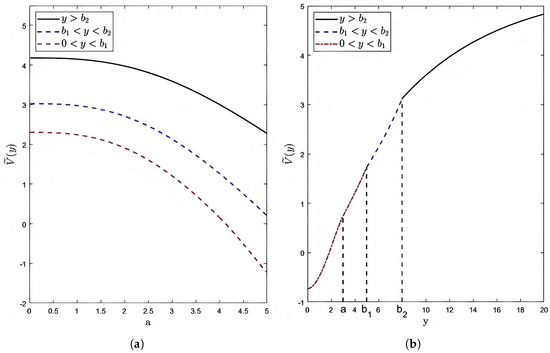
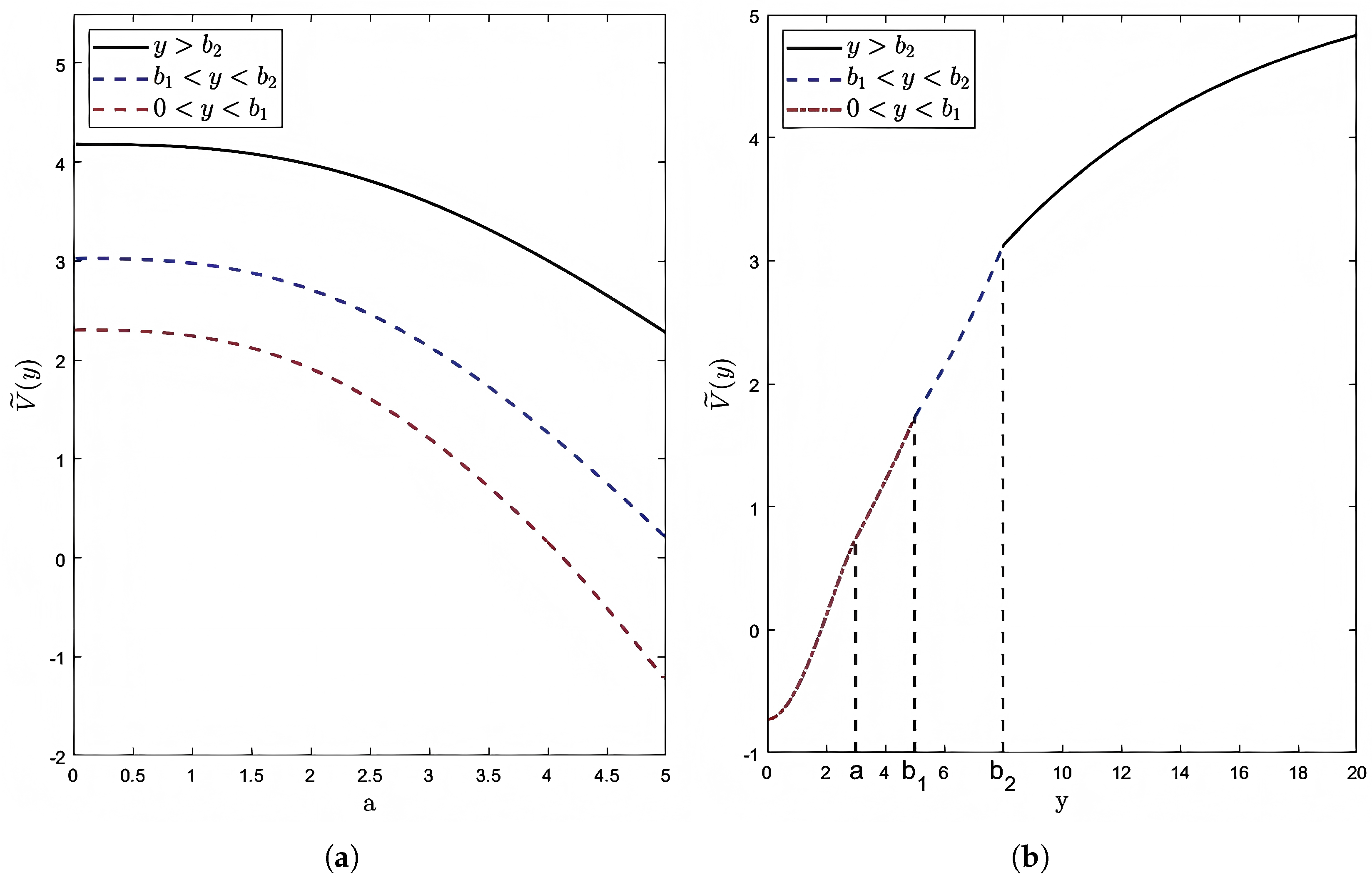
Figure 1 plots the curves of the value function $\tilde{V}\left(y\right)$ with respect to y and a, respectively. First, from Figure 1a, we observe that when the ratcheting dividend strategy barriers $b_1,b_2$, and the initial surplus y are fixed, $\tilde{V}\left(y\right)$ decreases as the random capital injection barrier a increases. Economically, a lower barrier a implies that capital injections occur more frequently, helping maintain solvency but also increasing the total discounted cost of those injections. Since the value function $\tilde{V}\left(y\right)$ is defined as the expected discounted cumulative dividends minus the expected discounted cumulative capital injections and the terminal value at ruin, more frequent injections reduce the net value, consistent with the observed decrease. The result that the optimal injection barrier is $a^{\ast }=0$ suggests that, under this model setup, it is economically suboptimal to delay capital injections—immediate injection when needed maximizes the net value.

Figure 1. The effect of a and y on $\tilde{V}\left(y\right)$: (a) when $b_1=5$, $b_2=8$, $y=10$ (solid and black) or $y=6$ (blue and dashed) or $y=4$ (red and dashed) for a∈$[0,b_1)$; (b) when $a=3$, $b_1=5$, $b_2=8$ for y∈$[0,20)$.

Figure 1b shows that the value function $\tilde{V}\left(y\right)$ increases with y and confirms that $\tilde{V}\left(y\right)$ is continuous in y. From an economic perspective, a higher initial surplus y reduces the need for external capital injections, thereby lowering the associated costs. At the same time, a larger surplus allows for higher cumulative dividend payments, which positively contribute to the value function. Hence, the increase in $\tilde{V}\left(y\right)$ with y reflects the net benefit of a stronger initial financial position.

4.1.2. The Effect of $b_1$ and $b_2$ on $\tilde{V}\left(y\right)$

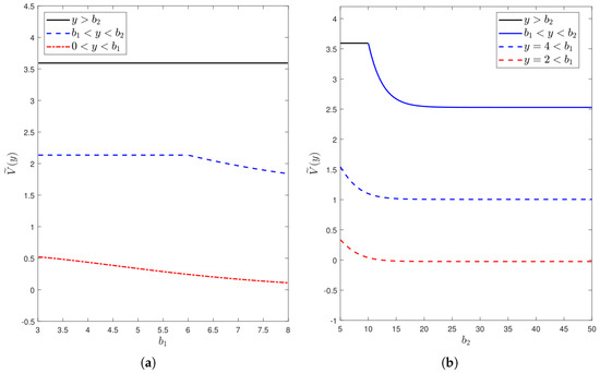
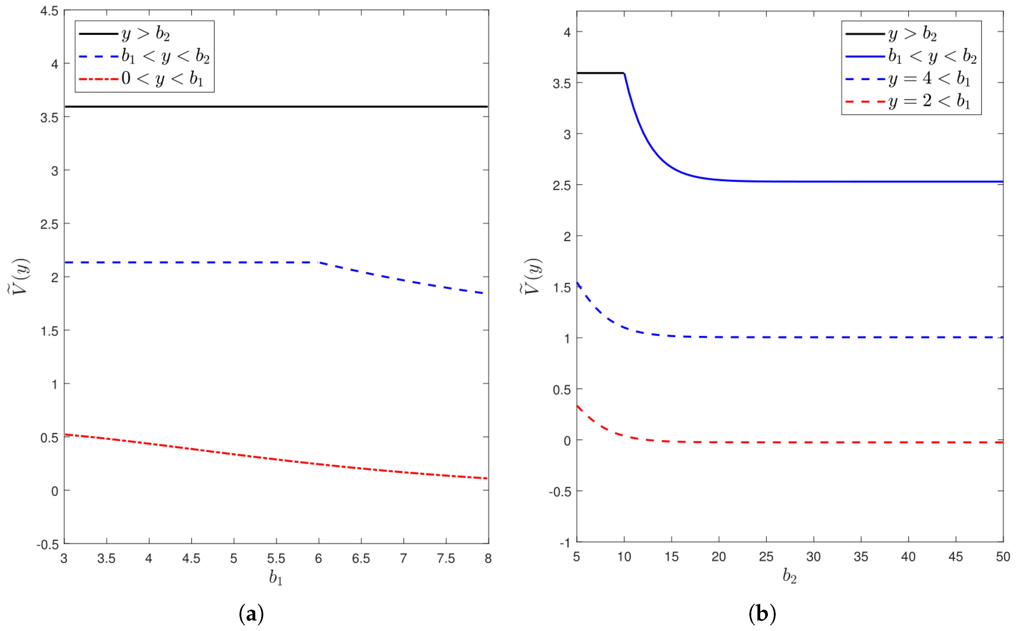
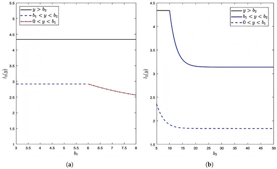
Figure 2 depicts the curves of the value function $\tilde{V}\left(y\right)$ with respect to the dividend thresholds $b_1$ and $b_2$. From Figure 2a, we find that the value function $\tilde{V}\left(y\right)$ is a decreasing function of $b_1$. Specifically, $\tilde{V}\left(y\right)$ remains constant when the surplus y exceeds the upper threshold $b_2$, while it exhibits an approximately linear relationship with $b_1$ when $y<b_2$. Economically, a higher $b_1$ raises the surplus level required to initiate dividend payments, thereby restricting both the frequency and the amount of dividends distributed. A reduction in dividends directly lowers $\tilde{V}\left(y\right)$, which aligns with the decreasing trend observed in the figure. The optimal lower dividend barrier is found to be $b_1^{\ast }=a$. This implies that, under the given framework, the dividend policy should be coordinated with the capital injection strategy: starting dividends only when the surplus reaches the same level a, which helps balance shareholder payouts with the firm’s solvency maintenance.

Figure 2. The effect of $b_1$ and $b_2$ on $\tilde{V}\left(y\right)$: (a) when $a=3$, $b_2=8$, $y=10$ (solid) or $y=6$ (dashed) or $y=6$ or 2 (dotted and dashed) for $b_1$∈$[a,b_2]$; (b) when $a=3$, $b_1=5$, $y=10$ (solid) or $y=4$ or 2 (dashed) for $b_2$∈$[b_1,50]$.

From Figure 2b, we observe that the value function $\tilde{V}\left(y\right)$ also decreases with $b_2$. When $y>b_2$, $\tilde{V}\left(y\right)$ stays constant, and as $b_2\to \infty$, it converges to a lower constant. In addition, the optimal upper barrier is obtained as $b_2^{\ast }=b_1$, indicating that, in this model, a multi-layer ratcheting dividend structure does not create additional value compared to a single-barrier strategy. This suggests that, under random capital injections, a simplified barrier dividend policy may be sufficient to maximize the value $\tilde{V}\left(y\right)$, as introducing a more complex ratcheting policy does not yield incremental benefits in terms of net expected discounted returns.

4.1.3. The Effect of $\gamma$, $c_1$, $c_2$ and $c_3$ on $\tilde{V}\left(y\right)$

Table 1, Table 2 and Table 3 list the values of $\tilde{V}\left(y\right)$ for different values of $\gamma$, $c_1$, $c_2$, and $c_3$, respectively. As seen from the horizontal values in Table 1, $\tilde{V}\left(y\right)$ first increases and then decreases as $c_1$ increases when fixing $\gamma =1.5$ and $\gamma =0.5$, while $\tilde{V}\left(y\right)$ is increasing when $\gamma =1$. The vertical values in Table 1 show that for any fixed $c_1$, $\tilde{V}\left(y\right)$ is an increasing function of $\gamma$. From Table 2, it can be obtained that for any fixed $\gamma$, $\tilde{V}\left(y\right)$ is an increasing function of $c_2$. And for any fixed $c_2$, $\tilde{V}\left(y\right)$ is also an increasing function of $\gamma$. The values in Table 3 show that $\tilde{V}\left(y\right)$ is monotonically increasing with respect to $c_3$ and $\gamma$, respectively. From the horizontal values in Table 2 and Table 3, it can be seen that the value of $\tilde{V}\left(y\right)$ varies slightly, which implies that the impacts of $c_2$ and $c_3$ on the value function are small. However, from the horizontal values in Table 1, we can see that the value of $\tilde{V}\left(y\right)$ varies greatly, which can conclude that the impact of $c_1$ on the value function is greater. The parameter $\gamma$ indicates the random decision time interval of capital injection, thus it is obtained that the shorter the random decision time interval, the larger the value function $\tilde{V}\left(y\right)$.

Table 1. The effect of $\gamma$ and $c_1$ on $\tilde{V}\left(y\right)$ when $b_2=8$, $b_1=5$, $a=3$ and $y=10$.

$\tilde{\mathit{V}}\left(\mathit{y}\right)$	${\mathit{c}}_1=$ 0.01	0.05	0.1	0.3	0.5
$\gamma =1.5$	2.51806	2.95146	3.44632	4.9693	−405,491.0
$\gamma =1$	2.64524	3.08763	3.59323	5.15464	6572.6
$\gamma =0.5$	2.83746	3.29256	3.8131	5.42302	2.6

Table 2. The effect of $\gamma$ and $c_2$ on $\tilde{V}\left(y\right)$ when $b_2=8$, $b_1=5$, $a=3$ and $y=6$.

$\tilde{\mathit{V}}\left(\mathit{y}\right)$	${\mathit{c}}_2=$ 0.01	0.05	0.1	0.3	0.5
$\gamma =1.5$	1.22727	1.55097	1.91364	3.00214	3.84767
$\gamma =1$	1.43186	1.76297	2.13426	3.25021	3.99072
$\gamma =0.5$	1.74197	2.08331	2.46622	3.6165	4.37548

Table 3. The effect of $\gamma$ and $c_3$ on $\tilde{V}\left(y\right)$ when $b_2=8$, $b_1=5$, $a=3$ and $y=4$.

$\tilde{\mathit{V}}\left(\mathit{y}\right)$	${\mathit{c}}_3=$ 0.01	0.05	0.1	0.3	0.5
$\gamma =1.5$	0.751465	0.837872	0.935416	1.22817	2.23615
$\gamma =1$	1.02726	1.11165	1.20698	1.49361	1.67849
$\gamma =0.5$	1.5945	1.66837	1.75184	2.00289	2.16159

4.2. Numerical Analysis of the Dividends Function $l_2\left(y\right)$ Without Capital Injections

We know $l_2\left(y\right)$ denotes the expected value of the discounted cumulative dividends at the ruin time for the spectrally negative Lévy process with a 2-layer ratcheting dividend strategy and without transaction costs. This section focuses on the analysis of $l_2\left(y\right)$ for a classical risk model. The specific results are mainly divided into two subsections, which show the impacts of the parameters y, $c_1$, $c_2$, $c_3$, $b_1$, and $b_2$ on $l_2\left(y\right)$, respectively.

4.2.1. The Effect of y, $c_1$, $c_2$, and $c_3$ on $l_2\left(y\right)$

Table 4, Table 5 and Table 6 state the values of $l_2\left(y\right)$ for $b_1=5$, $b_2=8$ and different values of y, $c_i$, $i=1,2,3$, respectively. By observing the horizontal values of each table, it is evident that $l_2\left(y\right)$ increases as $c_i$, $i=1$, 2, 3 increase when y is fixed. That is, in the absence of a random injection strategy, $l_2\left(y\right)$ is an increasing function of $c_i$, $i=1$, 2, 3. By observing the vertical values of each table, $l_2\left(y\right)$ increases as y increases. That is, when the initial surplus (reserves) increases, the moment when the surplus reaches the ratcheting dividend strategy barrier earlier, which means that the cumulative dividend amount increases.

Table 4. The effect of y and $c_1$ on $l_2\left(y\right)$.

${\mathit{l}}_2\left(\mathit{y}\right)$	${\mathit{c}}_1=0.01$	0.05	0.1	0.3	0.5	0.6
$y=10$	3.26925	3.76867	4.33658	6.0643	7.16474	7.56412
$y=6$	2.13994	2.50745	2.91627	4.11378	4.86427	5.13777
$y=2$	0.710863	0.936129	1.1828	1.87821	2.27543	2.406

Table 5. The effect of y and $c_2$ on $l_2\left(y\right)$.

${\mathit{l}}_2\left(\mathit{y}\right)$	${\mathit{c}}_2=0.01$	0.05	0.1	0.3	0.5	0.6
$y=10$	3.26925	3.76867	4.33658	6.0643	7.16474	7.56412
$y=6$	2.13994	2.50745	2.91627	4.11378	4.86427	5.13777
$y=2$	0.969948	1.0708	1.1828	1.51028	1.71122	1.78085

Table 6. The effect of y and $c_3$ on $l_2\left(y\right)$.

${\mathit{l}}_2\left(\mathit{y}\right)$	${\mathit{c}}_3=0.01$	0.05	0.1	0.3	0.5	0.6
$y=10$	3.26925	3.76867	4.33658	6.0643	7.16474	7.56412
$y=6$	2.54582	2.72047	2.91627	3.49264	3.84371	3.96788
$y=2$	1.11333	1.14608	1.1828	1.29088	1.35671	1.38

4.2.2. The Effect of $b_1$ and $b_2$ on $l_2\left(y\right)$

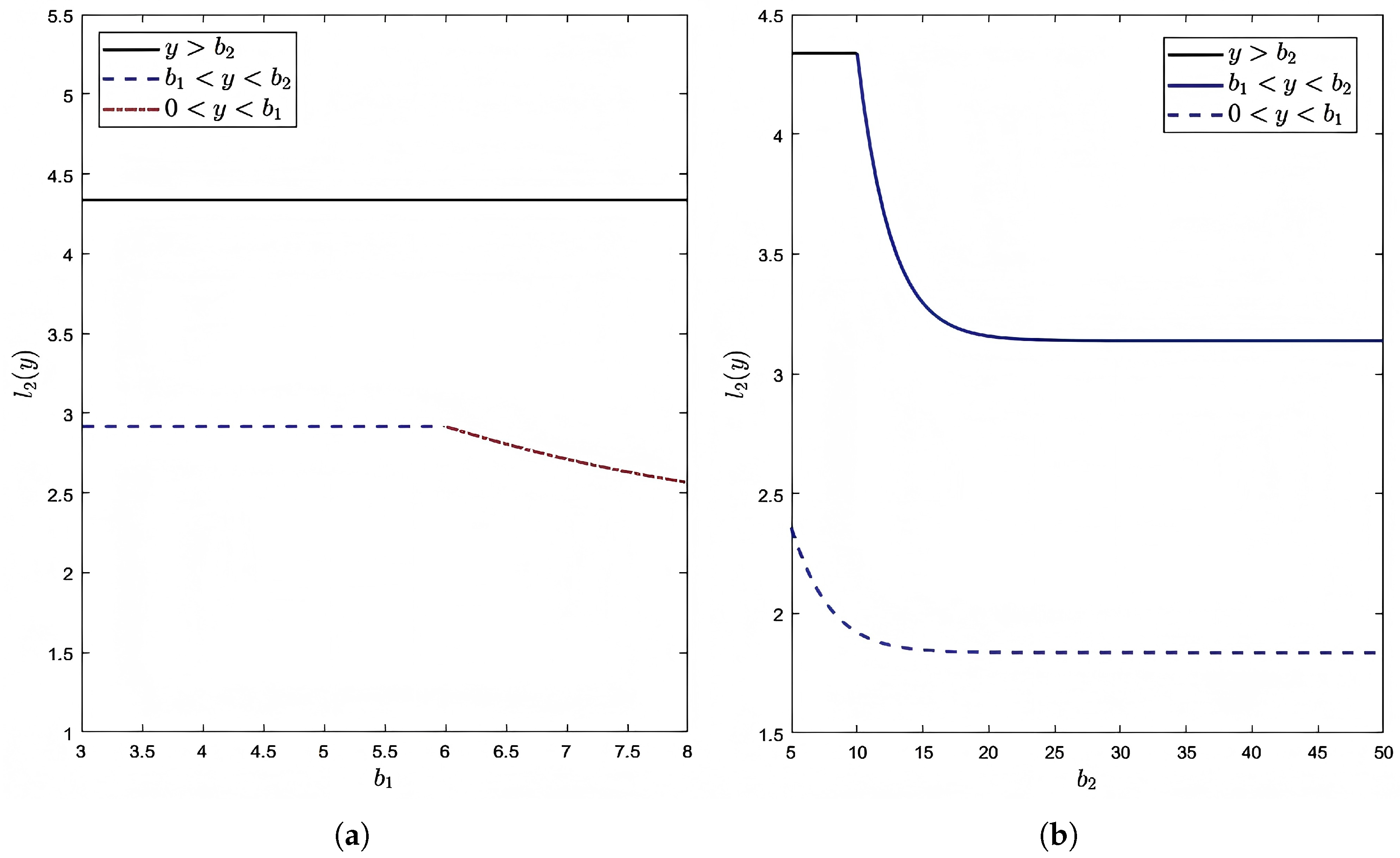
Figure 3 plots the curves of $l_2\left(y\right)$ with respect to $b_1$ and $b_2$. This is very similar to the curves in Figure 2. From Figure 3a, we see that $l_2\left(y\right)$ is constant when $y>b_2$ and $l_2\left(y\right)$ is a decreasing function of $b_1$ when $y<b_2$. More precisely, it is approximately a linear decreasing function of $b_1$ when $y<b_2$. The larger $b_1$, the smaller the dividends, resulting in a lower $l_2\left(y\right)$. From Figure 3b, $l_2\left(y\right)$ is constant when $y>b_2$, and $l_2\left(y\right)$ is a decreasing function of $b_2$ when $y<b_2$. In addition, when $b_2\to \infty$, $l_2\left(y\right)$ converges to a lower constant. It is also observed that the optimal ratcheting dividend strategy barrier is $b_2^{\ast }=b_1$, which indicates that the multi-layer ratcheting dividend strategy does not generate more dividends. Therefore, it is reasonable to conclude that the single-layer ratcheting dividend strategy is relatively better.

Figure 3. The effect of $b_1$ and $b_2$ on $l_2\left(y\right)$: (a) when $b_2=8$, $y=10$ (solid) or $y=6$ (dashed); (b) when $b_1=5$, $y=10$ (solid) or $y=4$ (dashed).

5. Conclusions

This paper focuses on two risk models: The spectrally negative Lévy risk model with the mixed n-layer ratcheting dividend strategy and the random capital injection strategy, and the spectrally negative Lévy risk model with the n-layer ratcheting dividend strategy. The corresponding value function, dividend function, capital injection function, and ruin function are expressed in terms of scale functions and related functions. Finally, we use a simple example to examine the effects of each parameter on the value functions and dividend functions.

For a two-layer ratcheting dividend strategy, the value function is a decreasing function of $\gamma$, a, $b_1$, $b_2$ and is an increasing function of y, $c_2$, $c_3$, and is a non-monotonic function with respect to $c_1$ in the presence of the random capital injection strategy, respectively. However, in the absence of the random capital injection strategy, the dividend function is an increasing function of y, $c_1$, $c_2$, $c_3$, and is a decreasing function of $b_1$ and $b_2$, respectively. In both cases (i) the value function and the dividend function converge to a constant when $b_2\to \infty$; (ii) the optimal ratcheting dividend strategy barrier corresponding to both the maximum value function and the maximum dividend function is $b_2^{\ast }=b_1$, which indicates that the multi-layer ratcheting dividend strategy does not generate more dividends. That is, in the presence of a random capital injection strategy, a single-layer ratcheting dividend strategy is relatively better than a multi-layer ratcheting dividend strategy.

References

- De Finetti, B. Su un’impostazione alternativa della teoria collettiva delrischio. In Proceedings of the Transactions of the XVth International Congress of Actuaries; International Actuarial Association: Ottawa, ON, Canada, 1957; Volume 2, pp. 433–443. [Google Scholar]
- Yang, H.; Zhang, Z. Gerber-Shiu discounted penalty function in a Sparre Andersen model with multi-layer dividend strategy. Insur. Math. Econ. 2008, 42, 582–593. [Google Scholar] [CrossRef] [Scilit]
- Yang, H.; Zhang, Z. On a perturbed Sparre Andersen risk model with multi-layer dividend strategy. J. Comput. Appl. Math. 2009, 232, 612–624. [Google Scholar] [CrossRef] [Scilit]
- Zhou, Z.; Xiao, H.; Deng, Y. Markov-dependent risk model with multi-layer dividend strategy. Appl. Math. Comput. 2015, 252, 273–286. [Google Scholar] [CrossRef] [Scilit]
- Xie, J.-H.; Zou, W. On the expected discounted penalty function for a risk model with dependence under a multi-layer dividend strategy. Commun. Stat. Theory Methods 2017, 46, 1898–1915. [Google Scholar] [CrossRef] [Scilit]
- Ragulina, O.; Šiaulys, J. Upper bounds and explicit formulas for the ruin probability in the risk model with stochastic premiums and a multi-layer dividend strategy. Mathematics 2020, 8, 1885. [Google Scholar] [CrossRef] [Scilit]
- Albrecher, H.; Bäuerle, N.; Bladt, M. Dividends: From refracting to ratcheting. Insur. Math. Econ. 2018, 83, 47–58. [Google Scholar] [CrossRef] [Scilit]
- Zhang, A.; Liu, Z. A Lévy risk model with ratcheting dividend strategy and historic high-related stopping. Math. Probl. Eng. 2020, 2020, 6282869. [Google Scholar] [CrossRef] [Scilit]
- Albrecher, H.; Azcue, P.; Muler, N. Optimal ratcheting of dividends in insurance. SIAM J. Control Optim. 2020, 58, 1822–1845. [Google Scholar] [CrossRef] [Scilit]
- Albrecher, H.; Azcue, P.; Muler, N. Optimal ratcheting of dividends in a Brownian risk model. SIAM J. Financ. Math. 2022, 13, 657–701. [Google Scholar] [CrossRef] [Scilit]
- Song, Z.; Sun, F. The dual risk model under a mixed ratcheting and periodic dividend strategy. Commun. Stat. Theory Methods 2023, 52, 3526–3540. [Google Scholar] [CrossRef] [Scilit]
- Gao, H.; Yin, C. A Lévy risk model with ratcheting and barrier dividend strategies. Math. Found. Comuput. 2023, 6, 268–279. [Google Scholar] [CrossRef] [Scilit]
- Sun, F.; Song, Z. Spectrally negative Lévy risk model under mixed ratcheting-periodic dividend strategies. Commun. Stat.-Simul. Comput. 2024, 53, 3186–3205. [Google Scholar] [CrossRef] [Scilit]
- Guan, C.; Xu, Z. Optimal ratcheting of dividend payout under Brownian motion surplus. SIAM J. Control Optim. 2024, 62, 2590–2620. [Google Scholar] [CrossRef] [Scilit]
- Sun, F.; Zhu, D. Spectrally negative Lévy risk model under ratcheting dividend strategy and capital injections with transaction costs. Commun. Stat. Theory Methods 2025, 55, 1246–1267. [Google Scholar] [CrossRef] [Scilit]
- Ren, X.; Wang, N. Optimal ratcheting dividend strategy with jump-diffusion risk process. Commun. Stat. Theory Methods 2025, 1–17. [Google Scholar] [CrossRef] [Scilit]
- Wang, W.; Xu, R.; Yan, K. Optimal ratcheting of dividends with capital injection. Math. Oper. Res. 2025, 50, 2073–2111. [Google Scholar] [CrossRef] [Scilit]
- Avanzi, B.; Shen, J.; Wong, B. Optimal dividends and capital injections in the dual model with diffusion. Astin Bull. 2011, 41, 611–644. [Google Scholar] [CrossRef] [Scilit]
- Yin, C.; Yuen, K.C. Optimal dividend problems for a jump-diffusion model with capital injections and proportional transaction costs. J. Ind. Manag. Optim. 2015, 11, 1247–1262. [Google Scholar] [CrossRef] [Scilit]
- Zhao, Y.; Chen, P.; Yang, H. Optimal periodic dividend and capital injection problem for spectrally positive Lévy processes. Insur. Math. Econ. 2017, 74, 135–146. [Google Scholar] [CrossRef] [Scilit]
- Avram, F.; Pérez, J.L.; Yamazaki, K. Spectrally negative Lévy processes with Parisian reflection below and classical reflection above. Stoch. Process. Their Appl. 2018, 128, 255–290. [Google Scholar] [CrossRef] [Scilit]
- Dong, H.; Zhou, X. On a spectrally negative Lévy risk process with periodic dividends and capital injections. Stat. Probab. Lett. 2019, 155, 108589. [Google Scholar] [CrossRef] [Scilit]
- Vinod, D.; Cherstvy, A.G.; Metzler, R.; Sokolov, I.G. Time-averaging and nonergodicity of reset geometric Brownian motion with drift. Phys. Rev. E 2022, 106, 034137. [Google Scholar] [CrossRef] [Scilit]
- Vinod, D.; Cherstvy, A.G.; Wang, W.; Metzler, R.; Sokolov, I.M. Nonergodicity of reset geometric Brownian motion. Phys. Rev. E 2022, 105, L012106. [Google Scholar] [CrossRef] [Scilit] [PubMed]
- Stojkoski, V.; Sandev, T.; Kocarev, L.; Pal, A. Geometric Brownian motion under stochastic resetting: A stationary yet nonergodic process. Phys. Rev. E 2021, 104, 014121. [Google Scholar] [CrossRef] [Scilit] [PubMed]
- Liang, Y.; Wei, Q.; Wang, W.; Cherstvy, A.G. Ultraslow diffusion processes under stochastic resetting. Phys. Fluids 2025, 37, 032014. [Google Scholar] [CrossRef] [Scilit]
- Loeffen, R.L.; Renaud, J.-F. De Finetti’s optimal dividends problem with an affine penalty function at ruin. Insur. Math. Econ. 2010, 46, 98–108. [Google Scholar] [CrossRef] [Scilit]
- Yin, C.; Wen, Y. Optimal dividend problem with a terminal value for spectrally positive Lévy processes. Insur. Math. Econ. 2013, 53, 769–773. [Google Scholar] [CrossRef] [Scilit]
- Kuznetsov, A.; Kyprianou, A.E.; Rivero, V. The Theory of Scale Functions for Spectrally Negative Lévy Processes; Springer: Berlin/Heidelberg, Germany, 2013; pp. 97–186. [Google Scholar]
- Kyprianou, A.E.; Loeffen, R.; Pérez, J.L. Optimal control with absolutely continuous strategies for spectrally negative Lévy processes. J. Appl. Probab. 2012, 49, 150–166. [Google Scholar] [CrossRef] [Scilit]
- Kyprianou, A.E. Fluctuations of Lévy Processes with Applications: Introductory Lectures; Springer Science and Business Media: Berlin/Heidelberg, Germany, 2014. [Google Scholar]
Disclaimer/Publisher’s Note: The statements, opinions and data contained in all publications are solely those of the individual author(s) and contributor(s) and not of MDPI and/or the editor(s). MDPI and/or the editor(s) disclaim responsibility for any injury to people or property resulting from any ideas, methods, instructions or products referred to in the content. |
© 2026 by the authors. Licensee MDPI, Basel, Switzerland. This article is an open access article distributed under the terms and conditions of the Creative Commons Attribution (CC BY) license.