


Abstract
– flavor reflection symmetry (RS) of the PMNS mixing matrix implies , leading to the atmospheric mixing angle and maximal Dirac CP violation phase, . Here, we establish an analytical connection between leptonic CP violation and the breaking of – RS through the effective flavor squared masses . We first examine the symmetric condition , which constrains to a highly localized weakly broken-RS geometric band, , centered at and over the continuous phase interval . The lower edge of the joint T2K–NOvA benchmark interval, , lies above this symmetric boundary (), motivating an extension to finite RS breaking. We therefore introduce the dimensionless RS-breaking indicator (RSBI), , and characterize the departure from RS through the – asymmetries and their flavor-asymmetry quadratic deviation . This leads us to conjecture that the physical value of the Dirac CP-violating phase corresponds to a minimum of . At leading-order, the resulting stationary condition provides a closed-form relation between and the three mixing angles. This leading order relation lies midway between the partial-symmetry results of Xing and Zhou. Evaluated at the empirical joint T2K–NOvA benchmark, the framework gives and , placing the phase in the third quadrant near-maximal CP violation. Including sub-leading corrections associated with the neutrino mass ordering gives the conditional estimates for Normal Ordering (NO) and for Inverted Ordering (IO), consistent with the corresponding direct numerical minimizations. These results suggest that may be constrained by collective relations among the neutrino mixing parameters rather than behaving as an entirely independent free parameter.
Keywords:
PMNS matrix; flavor neutrino mixing; effective neutrino masses; reflection symmetry breaking; CP violating phase MSC:
81R40; 81V15; 81V25
1. Introduction
Neutrinos are the most elusive stable particles in the universe [1]. Their importance within the Standard Model (SM) of particle physics has been increasing over time, often challenging the fundamental principles on which our understanding of nature is based [2,3]. A central issue concerns their possible role in determining the very existence of matter and the lack of an explanation for the observed matter-antimatter asymmetry in our world [4,5].
Within the SM, neutrinos are massless and are represented by three-flavor weak eigenstates , each associated with a charged-lepton partner, and denoted as , , and (see Supplementary Information (SI), Section S1). Remarkably, experimental evidence [6,7] requires the SM to be modified to allow neutrinos to acquire a finite mass, in such a way that each weak eigenstate is expressed as a superposition of three mass eigenstates . This mixing is described by the components of a complex unitary matrix, , known as the Pontecorvo–Maki–Nakagawa–Sakata (PMNS) matrix [8,9,10]. In the case of Dirac neutrinos, the mixing matrix is parameterized by three mixing angles, , and a single Dirac CP-violating phase, . While the mixing angles are currently determined to within (2–6)%, the uncertainty in remains significantly larger, spanning (40–80)% of the full range (see below). A compelling question is whether underlying flavor symmetries could effectively reduce the number of these independent parameters [11,12].
As a result of the mixing, the flavor composition of a neutrino evolves as it propagates; consequently, upon detection, it may manifest a different flavor from the one it possessed at production. This process results in the phenomenon of neutrino oscillations, the probability of which depends on the squared-mass differences, , , and the elements of the matrix. These oscillations are further modulated by the neutrino energy, , and the propagation distance, L (the baseline) (see SI, Section S2). Although experiments have provided significant insight into neutrino masses and mixing parameters over recent decades [13], several fundamental questions remain open. This is especially true regarding the precise values of the matrix elements, which are essential for characterizing CP violation in the lepton sector [14,15,16,17,18,19,20].
Experiments involving neutrino oscillations enable the determination of squared-mass splittings with high precision; however, the neutrino mass ordering remains a primary challenge. While recent joint terrestrial analyses of NOvA [15] and T2K [17] data indicate a slight statistical preference for the Inverted Ordering [18], cosmological analyses incorporating DESI observations have reported stringent, model- and dataset-dependent upper limits on the neutrino mass sum, including values as low as eV [19]. Such constraints can create tension with the minimum mass sum required for Inverted Ordering, approximately eV, within the adopted cosmological framework. However, this tension should not be interpreted as a model-independent exclusion of Inverted Ordering [20]. Furthermore, the underlying nature of either – exchange symmetry (ES) or reflection symmetry (RS), extended to their broken counterparts, remains a subject of intense theoretical investigation [21,22,23,24,25,26,27]. Within this framework, we focus exclusively on Dirac neutrinos, which are predicted to possess distinct electromagnetic properties, including magnetic and electric dipole moments as well as minute electric charges, or millicharges [28,29].
Motivated by these developments, and specifically by the substantial uncertainty surrounding , we explore a link between CP violation and a broken – flavor RS, suggesting that the actual variability of may be significantly more constrained than currently assumed. Using effective flavor squared-masses as a starting point, we first derive a new relation expressing as a function of the three mixing angles and two squared-mass splittings, under the assumption that the here defined RS breaking indicator (RSBI), , where , takes the value , consistent with unbroken RS here in the case and . In fact, yields a narrow weakly broken RS geometric band of values centered at for in the range (Normal Ordering) and the mirrored range for Inverted Ordering. Specifically, we find
where the maxima and minima of this interval correspond to the vanishing of CP violation, i.e., . The quoted uncertainties represent propagated uncertainties in the input oscillation parameters, assumed to be independent (see Appendix B.3). However, the most recent joint T2K–NOvA experimental estimates [18] indicate
The lower edge of the experimental benchmark interval in Equation (2) lies above the upper boundary of the theoretical interval in Equation (1). However, the latter is obtained under the specific condition and should not be interpreted as an experimental confidence interval. Consequently, this comparison does not, by itself, establish a statistically significant discrepancy with – reflection symmetry. Instead, it motivates extending our analysis to a non-vanishing RSBI, , accounting for finite effective flavor squared-mass differences, , consistent with broken RS. Through a detailed examination of the flavor-asymmetry quadratic deviation of the – asymmetries , we are led to formulate the following conjecture:
As a result, we derive an analytical prediction for cos(δCP) terms of the three mixing
angles,
Using the current joint T2K–NOvA experimental values [18], sin2 θ12 = 0.307 ± 0.013 and sin2 θ13 = 0.0218 ± 0.0008, the prefactor multiplying cot(2θ23) becomes 1.447 ± 0.143, and taking
= , the following values are obtained:
where
is roughly one-tenth the atmospheric mass scale, ≃ 2.5 × 10⁻³ eV2, thus suggesting that RS is only slightly perturbed, and
This conditional estimate, based on the joint T2K–NOvA benchmark [18], places the Dirac CP-violating phase near-maximal CP violation within the phenomenological framework adopted here.
The remainder of this paper is organized as follows: In Section 2, we outline the procedure for dealing with the mass eigenvalues , explicitly formulate the standard form of the matrix, and discuss the effective flavor masses. In addition, we discuss the issue of CP violation, ES and RS flavor symmetries, and the exact evaluation of the flavor-asymmetry quadratic deviation . Section 3 analyzes CP violation in the case , its connection with – RS, and making contact with the joint T2K–NOvA experimental results [18]. In Section 4, we extend the analysis to non-vanishing RSBI, (), consistent with broken RS. We discuss the possibility of near-maximal CP violation, which leads to the primary analytical result of this study. In Section 5, we compare our analytical correlation with the NuFIT 6.1 two-dimensional likelihood distributions for both neutrino mass orderings, providing a quantitative assessment of its compatibility with current global oscillation data. Finally, Section 6 provides our concluding remarks.
2. Mass Eigenstates and the PMNS Matrix
2.1. Mass Eigenstates
We briefly summarize the input data used in this study [18], starting with the squared-mass differences presented in Table 1. In the Normal Ordering (NO) scenario, given the smallest mass , the values of and are obtained via
whereas for Inverted Ordering (IO), given , the remaining masses are given by
Table 1.
Squared-mass differences, . For NO, one has , while for IO, , therefore, in this case. The third row shows the sum when the lightest mass vanishes: for NO and for IO. The last row corresponds to the lightest mass: eV (NO) and eV (IO) [29]. These sums are to be compared with (DESI) eV. All masses are in eV.
To facilitate comparison with cosmological observations, it is customary to set the lightest neutrino mass to zero. For the NO case, using Equation (3) and the relation , we obtain
resulting in a total mass sum of meV. Conversely, Equation (4) yields
leading to meV (as shown in the third row of Table 1).
Under the cosmological assumptions and dataset combination leading to the illustrative DESI-related bound meV, Inverted Ordering is strongly constrained because its minimum mass sum is approximately 99 meV. Normal Ordering remains compatible with this particular bound for sufficiently small values of the lightest neutrino mass. For instance, taking meV gives meV, which remains below the illustrative 64 meV bound. These conclusions are conditional on the cosmological model and observational inputs and should not be interpreted as universal constraints on the neutrino mass ordering. Furthermore, a lower bound for Dirac neutrino masses of meV has recently been proposed based on phenomenological arguments [29]. The mass sums corresponding to this lower bound for both NO and IO are listed in the fourth row of Table 1; these remain compatible with the illustrative DESI-related constraint only in the NO case.
2.2. PMNS Matrix
The PMNS matrix is a unitary mixing matrix that describes the misalignment between the flavor and mass eigenstates of neutrinos, which governs their oscillation during propagation. This framework was introduced by Maki, Nakagawa, and Sakata [8] to describe the neutrino oscillations originally hypothesized by Pontecorvo in 1957 [9]. The matrix is conventionally parameterized by three mixing angles (, , and ) and a Dirac CP-violating phase (),
where and . It is given by the product of three Euler rotation matrices (, , ) and a diagonal matrix containing the Dirac phase (1, 1, ), according to . The current best fits for the angles and phase are reported in Table 2.
Table 2.
Numerical values of the four parameters entering the PMNS matrix as reported in the joint T2K–NOvA analysis [18]. The quoted uncertainties correspond to 1 (68.27%) intervals, while the separate NO and IO ranges for correspond to 3 (99.73%) Bayesian credible intervals [18]. When no mass ordering is assumed, the 1 credible interval for the CP phase is , with highest posterior probability at .
For N generations of Dirac fermions, an arbitrary unitary mixing matrix contains real parameters, of which correspond to mixing angles. The remaining parameters are phases. However, not all of these phases are physical. Rephasing the left-handed and right-handed fermion fields allows phases to be absorbed, since one common rephasing leaves the mixing matrix unchanged. Therefore, the number of remaining physical CP-violating phases is
For , there are no CP-violating phases, while for , one has corresponding to a single phase, in our case, the Dirac phase . The eventual existence of an additional condition on would therefore reduce the number of free parameters to just three effectively independent parameters. In this work, we investigate such a possibility.
As is apparent from Table 2, the allowed ranges for in both the NO and IO scenarios include the special case , which corresponds to maximal CP violation. The degree of violation is quantified by the Jarlskog invariant, originally suggested for the quark sector [30,31]. For neutrinos, it is given by (see e.g., [32,33])
yielding the well-known expression
which provides a parameterization-independent measure of CP violation. For , this yields . Conversely, if , CP symmetry is preserved. Notably, for NO, both and lie within the reported 3 credible interval. For IO, however, the corresponding interval from the joint T2K–NOvA analysis [18] excludes these CP-conserving values, thus favoring finite leptonic CP violation within that analysis (see also [33,34]).
To facilitate our analysis, we consider the squared absolute values of the PMNS matrix elements, , where and denote the flavor and mass indices, respectively. From Equation (7), we obtain
where and . These elements satisfy the standard unitarity conditions:
2.3. Effective Flavor Neutrino Masses
The effective neutrino mass-squared matrix in the flavor basis, (also denoted as ), where , is discussed in Appendix A. The diagonal elements of are denoted as the effective flavor neutrino squared-masses
The quantity is of particular experimental importance; for instance, the KATRIN experiment [35] utilizes the electron neutrino effective mass, , to constrain the scale of neutrino masses, currently suggesting eV (90% CL) (see SI, Section S2.4). From Equations (17) and (18), it follows that the sum of the effective squared-masses over all flavors satisfies
By substituting the squared moduli of the electron-row PMNS matrix elements from Equation (10) into Equation (18), the effective electron neutrino squared mass can be written as
Unless otherwise stated, the symbol refers to the effective electron neutrino mass (see also SI, Section S2.4). For the two possible mass orderings, this relation can be expressed in terms of the squared-mass differences as follows:
Assuming the lightest mass vanishes ( for NO and for IO), we use the best-fit values from Table 1 and Table 2 to estimate :
where the correspondence with the mass eigenstates and refers back to Equation (5) and Equation (6), respectively. These results are illustrated schematically in Figure 1.
Figure 1.
Schematic representation of the Normal Ordering (NO, left panel) and the Inverted Ordering (IO, right panel). The vertical blue lines denote , and the red lines denote (cf. Table 1). The red circles indicate the effective electron neutrino mass values, , for the case where the minimum mass vanishes (Equations (23) and (24)). The effective flavor masses (blue circles) and (yellow circles) have been calculated employing the expressions in Appendix B.1 and are positioned according to their respective orderings. See Supplementary Information for additional details.
One can wonder how the effective flavor masses, , and , and the mass eigenstates depend on the absolute mass scale as a function of the smallest mass eigenstate value, for NO and for IO (cf. Figure 1). We employ Equations (A10) and (A11) to obtain the effective flavor masses and , and Equations (21) and (22) for the effective electron flavor mass , as a function of the lightest mass eigenstate. Illustrative results for are shown in Figure 2. Notably, remains close to in the NO case and to in the IO case as the reference mass scale increases, while for both orderings. In the limit of larger (NO) or (IO), all six mass scales approach a quasi-degenerate regime (see also [29]).
Figure 2.
Mass eigenstates and effective flavor neutrino masses vs. the lightest mass eigenvalue. (a) NO, where is the lightest eigenmass; (green line) essentially coincides with (black circles), (blue line) (yellow line), and (red circles) is the heaviest state. (b) IO, with as the lightest mass; (green line) nearly coincides with (black circles), both of which remain below the heaviest mass (red circles), and . For illustration, we assume with remaining parameters taken from Table 1 and Table 2. All masses are in meV.
Interestingly, an effective mass ordering also emerges for the three flavors. Specifically, for the NO eigenmass ordering (Figure 2a), the effective flavor masses follow an IO-type sequence where . Conversely, for the IO eigenmass ordering (Figure 2b), an NO-type sequence occurs, with . This flavor ordering remains robust for all values of , provided the atmospheric mixing angle obeys (see Section 3).
To explore other regions of the parameter space, we allow to vary while keeping the remaining parameters fixed according to Table 2. Illustrative results are presented in Figure 3, demonstrating that, within a narrow interval around (approximately –), the difference changes sign. The exact values of where depend on the choice of . Consequently, when the condition is met, the CP phase can be expressed as a function of the other three mixing angles. Notably, as approaches , the zeros for both NO and IO converge at .
Figure 3.
Mass differences between effective flavor masses, () [meV] vs. [degrees], with and held fixed (cf. Table 2). The plots show NO results (black lines), IO results (red lines), (dashed lines), and (solid lines). The blue lines are guides to the eyes.
2.4. Lagrangian Symmetries and Flavor-Asymmetry Quadratic Deviation
In this section, we make contact with the issue of Lagrangian symmetries from which the roadmap of the main result of the paper is highlighted (Section 2.4.1), followed by the introduction of the central quantity, i.e., the flavor-asymmetry quadratic deviation in Section 2.4.2.
2.4.1. – Exchange and Reflection Symmetries
In the minimal SM, no RH (LH) neutrino (antineutrino) field is present, consistent with decay observations illustrated in SI, Figure S1. Therefore, in contrast to charged leptons and quarks, neutrinos cannot acquire a Dirac mass through the ordinary Higgs mechanism since it requires the existence of RH neutrinos and LH antineutrinos (see [29] for an alternative mechanism for neutrino mass). To accommodate massive Dirac neutrinos, the SM field content must therefore be extended by introducing three electroweak-singlet RH fields .
As discussed in SI, Section S3.3, the Yukawa interaction generates the Dirac neutrino mass term represented by the Dirac mass Lagrangian,
where and is the Dirac mass matrix, which in general is neither symmetric nor Hermitian. For studying neutrino oscillations, it is particularly convenient to introduce the Hermitian mass-squared matrix defined in Appendix A:
This formulation is further developed in SI, Section S3.3, to discuss – flavor exchange symmetry (ES; SI Section S3.3.1) and reflection symmetry (RS; SI Section S3.3.2) within the Dirac-neutrino scenario. Here, we adopt RS as our candidate ‘unperturbed’ symmetry state, for which and ; in the following, we consider the branch, corresponding to maximal CP violation and finite mixing angles . In contrast, ES yields , in contradiction with experimental results, thus keeping fully undetermined.
Therefore, our strategy is to adopt exact – reflection symmetry as a reference configuration and investigate departures from it through the properties of the mass-squared matrix in the flavor basis, , whose off-diagonal elements are directly related to CP violation, as shown in SI, Section S3.2. Furthermore, the condition for full – RS is defined by the equality [21,23]
an immediate consequence particularly relevant to the present analysis is, as we discuss in detail in Section 3,
and therefore
Thus, exact – RS necessarily implies equality of the effective squared masses associated with the - and flavors:
However, while this equality is a necessary consequence of RS, it is not sufficient to establish the full symmetry. Indeed, as shown in Section 3, the condition may also be satisfied away from the exact-RS point, where the individual relations do not hold. We find an exact periodic functional relation between and , in which the atmospheric angle obeys (see Equations (36) and (37)), with .
2.4.2. Flavor-Asymmetry Quadratic Deviation:
As mentioned in Section 2.2 regarding the PMNS mixing parameters, we investigate whether an additional condition on could reduce the number of independent mixing parameters to three, for example, the three angles , , and . To explore this possibility, we consider the flavor asymmetries
and seek a collective measure to characterize their dependence on the CP-violating phase , initially keeping the three mixing angles fixed at their experimental values reported in Table 2. We therefore quantify the combined asymmetry by defining the flavor-asymmetry quadratic deviation
Here, by unitarity of the PMNS matrix (see Equation (17)). To clarify the meaning and behavior of , we first consider the exact-RS mixing-angle limit , obtaining the simple result derived in Section 3:
where and have been assumed. In the exact-RS limit, the absolute minima of occur precisely at . Away from this limit, for , the location of the minimum may shift from . We propose that this shifted minimum can provide a phenomenological estimate of the physical Dirac phase, particularly for small departures from the exact-RS mixing angle . This extension is a conjecture, not a consequence of the exact-symmetry result.
These considerations motivate the following phenomenological conjecture concerning the PMNS mixing parameters:
A derivation of this conjecture from an underlying dynamical or flavor-symmetry framework remains an open problem.
To implement conjecture (31), we quantify departures from the equality using the RS-breaking indicator , introduced in Section 4. For broken RS (), we implement conjecture (31) by minimizing the quadratic deviation along the curve defined by a fixed value of , with varying consistently with . The leading-order analytical approximation and the exact constrained stationary-point relation are derived in Section 4.3.1 and Section 4.3.2, respectively.
3. CP Violation Condition in the Case
In the following, we seek to establish a relationship between and as a function of , , and the squared-mass differences , particularly focusing on cases near-maximal CP violation (). Building on the results illustrated in Figure 2 and Figure 3, we explore configurations exhibiting a form of – RS [21,23]. Specifically, we adopt the RS indicator condition, , as a generalization of the full RS requirement of Equation (26).
3.1. Relation Between and
Related correlations between atmospheric mixing and leptonic CP violation have also been investigated within partial – symmetry frameworks, notably by Xing and Zhou [22]. In the present approach, we instead impose equality of the effective flavor squared masses, , which leads to the constraint derived below. According to Equation (20), the electron neutrino effective squared-mass is independent of both and , whereas and depend on both parameters. By imposing the condition and utilizing Equations (11)–(16), we derive the following relation for (detailed derivations are provided in Appendix B.1):
where
This expression is noteworthy because, under the imposed effective flavor squared-mass equality condition, it establishes a correlation between and , thereby reducing the number of independent mixing parameters from four to three within this constrained framework. Furthermore, the condition factorizes the dependence of into two distinct components: one purely dependent on and another on the remaining mixing angles and mass splittings. In Appendix B.2, we verify that the condition is obeyed within the band given by (32).
For our purposes, it is more convenient to express explicitly as a function of the phase , keeping the remaining parameters fixed (refer to Appendix B.1 for derivation details):
where
This can be stated more compactly (cf. Equations (A18) and (A19)) as
where . Relation (36) holds provided that , which restricts the range of around . This behavior is illustrated in Figure 4, where we examine Equation (34) as a function of using the values from Table 1 and Table 2.
Figure 4.
The condition on CP violation. The atmospheric angle [°] vs. [°], using Equations (34) and (35). Maximal CP violation occurs at , yielding (green circle). Solid lines represent the experimentally determined ranges of for NO (black) and IO (red) reported in Ref. [18] (see Table 2). The dashed lines indicate the theoretical upper () and lower () boundaries, corresponding to (green squares). The propagated uncertainties of approximately (dark-green squares) in these boundary locations are discussed in Appendix B.3. The green and pink lines are guides to the eyes.
We consider both the NO and IO cases as discussed in [18]. While the NO case exhibits a broader range for due to current experimental uncertainties, the behavior of remains fully consistent with the narrower IO regime; indeed, is contained within the same numerical limits for both orderings. Specifically, we find
The uncertainties of approximately associated with the theoretical boundary values in Equation (37) correspond to propagated uncertainties in the input oscillation parameters, treated as independent. These uncertainties characterize the locations of the geometric boundaries under the condition and should not be confused with experimental confidence intervals for . Details of the analytical uncertainty propagation and numerical parameter variations are provided in Appendix B.3. This range is consistent with the results shown in Figure 3 (dashed lines), where the bounds correspond to and . We conclude that, within this narrow range of , the condition can be satisfied provided that obeys Equation (36). Away from the exact-RS point, this equality corresponds to a departure from full reflection symmetry, since the individual matrix elements generally satisfy . Exact RS is recovered at and (see also Section 3.2).
The narrow interval in Equation (37) represents a theoretical geometric boundary obtained under the specific condition , or equivalently , with the remaining oscillation parameters fixed at their adopted reference values. It should therefore not be interpreted as an experimentally determined confidence interval for . In particular, its comparison with the benchmark atmospheric mixing range reported in Table 2 does not, by itself, establish a statistically significant tension with – reflection symmetry. Rather, atmospheric mixing angles lying outside this conditional boundary motivate the more general scenario of non-vanishing effective flavor squared-mass asymmetry, , which we investigate in Section 4.
3.2. Matrix Elements and Under the Condition
The condition does not intrinsically imply (for ) (see the closing discussion in SI, Section S3.3.2). Instead, the components of the PMNS matrix for and generally differ. To illustrate this behavior, we plot the differences Equation (28), using the results from Appendix C.2, as a function of the phase in Figure 5, for both Normal Ordering (NO, solid lines) and Inverted Ordering (IO, dashed lines).
Figure 5.
Differences vs. [°] for Normal Ordering (solid lines) and Inverted Ordering (dashed lines), using the expressions (11)–(13) for and (14)–(16) for . The values for and are from Table 2 and squared-mass differences from Table 1. The angle is determined via Equations (34) and (35). The values for have been multiplied by 15 for clarity. The dashed and continuous brown lines are guides to the eyes.
Note that the differences for have been scaled by a factor of 15 for clarity, due to the fact that for the numerical configurations considered. We observe the following approximate relations between the flavor asymmetries for normal and inverted mass orderings:
For the symmetric configurations considered, all three flavor asymmetries vanish at exactly , where , corresponding to exact – reflection symmetry and maximal Dirac CP violation. Conversely, their absolute magnitudes reach their maximum values at , corresponding to CP-conserving phases.
Figure 6 shows that the quadratic deviation reaches its absolute minimum, , at , corresponding to maximal mixing . This result is consistent with the analytical expression derived for the symmetric case, Equation (30), obtained from the analytical results presented in Appendix C.2. More importantly, it provides a phenomenological motivation for the conjecture introduced in (31). In particular, the equality is consistent with maximal CP violation in the exact-RS limit, although this equality alone does not constitute a sufficient condition for exact reflection symmetry.
Figure 6.
The global flavor-asymmetry quadratic deviation as a function of the Dirac CP phase , evaluated for the configurations presented in Figure 5. For both NO (black solid line) and IO (red dashed line), the absolute minimum occurs at (red circle). The two curves are practically indistinguishable and closely approximate the analytical expression for given in Equation (30), which is exact for . The thin vertical lines are included as visual guides.
4. Impact of the – Mass Asymmetry on the CP-Violating Phase: The RSBI
As discussed in Section 3.1, the current experimental results for (Equation (2)) suggest that – RS, and maximal CP violation, may be broken. To improve the theoretical estimates of , we extend our previous framework to the more general case of finite . Under these conditions, the relationship between and is generalized to,
where is the RSBI, which characterizes the degree of RS breaking. In the limit , (41) reduces to Equation (36), or equivalently to Equations (34) and (35) (see Appendix C.1 for the full derivation).
4.1. Maximal CP Violation:
Let us first consider the case of maximal CP violation, . From Equation (41), we obtain
which allows us to determine the symmetry-breaking parameter from the experimental value . We find that the ratio is negative for both Normal (NO) and Inverted (IO) orderings. Specifically, for NO, we have and , whereas for IO, we find and . Given that , we can approximate Equation (42) using a Taylor expansion:
This can be expressed as a shift from the maximal mixing case:
where , and the deviation is given by
Using the current experimental value degrees (see Table 2), we apply Equation (42) to determine the symmetry-breaking parameter . This yields
We observe that , which is consistent with our perturbative expectations. In addition, the fact that is roughly an order of magnitude smaller than the atmospheric mass scale, , suggests that RS is indeed a “good” symmetry that is only slightly perturbed. It is interesting to note that is actually independent of the absolute neutrino mass scale as shown in Appendix D.
4.2. Near-Maximal CP Violation:
In the general case where , the first term on the right-hand side of Equation (41) remains bounded according to
which establishes a narrow, finite CP-violation band centered at .
To proceed further, we expand the mixing angle about the symmetry-preserving limit by substituting
into Equation (41). Defining and adopting for simplicity the shorthand notation , this yields
By exploiting the boundary condition that defines the unperturbed state, namely,
Equation (50) simplifies directly to
It is worth noting that in the limit of maximal CP violation (), the unperturbed angle becomes . Under these conditions, Equation (51) yields , which can be Taylor expanded as , in perfect agreement with Equation (45).
We can express the result in Equation (51) in a more compact form by simplifying the prefactor in parentheses using the identity from Equation (34):
which allows Equation (51) to be written as
Solving directly for the deviation yields
Given that (see Figure 4), it follows that from Equation (45). Expanding about this limit, we arrive at our final analytical estimate for the mixing angle:
The second term on the right-hand side of Equation (55) induces a highly constrained band of width (cf. Section 3) around the primary shift . Figure 7 displays vs. , illustrating plausible physical scenarios across a range of values.
Figure 7.
The mixing angle [°] derived from Equation (55) plotted against the CP-violating phase for various selections of the symmetry-breaking parameter (continuous lines), where for Normal Ordering and for Inverted Ordering. The benchmark case of for NO (red line) ( for IO (red dashed line)) is highlighted, matching the experimental central value (orange circle including the experimental error bars), which corresponds to a net symmetry-breaking deviation of . The thin red and green lines are guides to the eyes.
The orange circle represents the experimental baseline, , positioned at for visual clarity. Note that within this framework, any value of the CP phase is theoretically permissible across the entire interval (indicated by the red lines). In the following section, we apply our conjecture (31) to lift this degeneracy, thereby substantially narrowing the allowed range of .
4.3. Matrix Elements and Under the Condition
Let us analyze the behavior of the PMNS matrix elements under the broken RS framework as illustrated in Figure 8 in terms of the flavor asymmetries defined in Equation (28).
Figure 8.
Flavor asymmetries as functions of under broken symmetry (), for Normal Ordering (NO, solid lines) and Inverted Ordering (IO, dashed lines). Black, red, and green curves correspond to the mass eigenstates , respectively. The atmospheric mixing angle is determined from the exact fixed- constraint, Equation (41), using the empirical benchmark values from Equations (46) and (47). The inset magnifies the weak phase dependence of , highlighting the crossing of the NO and IO curves at .
An interesting feature of Figure 8 is the markedly different dependence of the three flavor asymmetries on the CP-violating phase. In particular, the asymmetry exhibits only a weak variation with , as highlighted in the inset, where the NO and IO curves intersect at . This crossing follows from the common experimental benchmark adopted for both mass orderings at maximal CP violation. Despite its weak phase dependence, provides a substantial contribution to the quadratic deviation , thereby influencing its overall magnitude. Conversely, the stronger phase dependence of and plays a major role in determining the location of the minimum of . Thus, the three asymmetries contribute differently to the magnitude and phase dependence of the collective departure from – reflection symmetry.
As illustrated in Figure 8, introducing a finite lifts the approximate NO–IO degeneracy of the flavor-asymmetry magnitudes observed in the symmetric case (cf. Figure 5). Nevertheless, the distinct phase dependences exhibited in Figure 8 reflect an underlying analytical relationship between the CP-violating phase and the mixing angles , as discussed below.
As derived in Appendix C.2, the flavor-asymmetry quadratic deviation , defined in Equation (29), takes the explicit form:
where [cf. Equation (50)], and the structural prefactors are given by
The curves shown in Figure 9 are calculated by evaluating the quadratic deviation with the atmospheric mixing angle determined from the exact fixed- constraint, Equation (41). The resulting landscape exhibits three stationary points: two trivial solutions at , corresponding to local maxima at the boundaries of the selected phase interval, and a non-trivial interior minimum located near .
Figure 9.
The flavor-asymmetry quadratic deviation as a function of the CP-violating phase , evaluated for the broken-symmetry configurations presented in Figure 8 using the exact fixed- constraint, Equation (41). The numerical minima occur at for Normal Ordering (NO) and for Inverted Ordering (IO). In the symmetric limit (), the minimum occurs at (cf. Figure 6).
4.3.1. Conjecture on : Analytical Relation Between and the Mixing Angles
To determine the non-trivial variational solution for the CP phase, we evaluate the extremum condition of the flavor-asymmetry quadratic deviation with respect to , namely, . To simplify this calculation, we observe that depends explicitly on the phase via the parameter and implicitly through the functional dependence of established in Equation (41). The total derivative can therefore be expanded as
Here, the total derivative is evaluated along the fixed- constraint, with all other oscillation parameters held constant. As a first approximation, we neglect the implicit dependence of on when evaluating the stationary condition. This fixed-angle approximation isolates the explicit phase dependence of and leads to a simple analytical correlation. Its accuracy can be assessed by comparison with the exact constrained minimization developed in Section 4.3.2. Consequently, we isolate the dominant physical behavior by adopting the leading-order approximation:
Differentiating Equation (56) under this assumption yields
The prefactor immediately recovers the trivial boundary solutions . Setting the bracketed terms to zero isolates the non-trivial stationary state, therefore yielding . Substituting the definitions of the structural parameters from Equation (58), we arrive at the fundamental analytical relation
Evaluating the leading-order correlation Equation (62) using the empirical central values of the mixing angles from Table 2 yields the conditional estimate
for both Normal and Inverted Orderings, in excellent agreement with the ordering-dependent numerical minima shown in Figure 9, within the accuracy of the leading-order approximation. The stated statistical uncertainties are predominantly driven by the experimental error on (cf. Table 2). Notably, Equation (62) correctly reduces to the unbroken RS limit, , as the atmospheric mixing angle approaches the maximal configuration .
4.3.2. Exact Stationary-Point Correlation by Minimization at Fixed
Within the proposed minimization conjecture, the following exact constrained calculation establishes a correlation between the stationary values of and , rather than an independent prediction of either parameter. To this end, we consider the flavor-asymmetry quadratic deviation subject to the exact constraint Equation (41)
with and , where is given in Equation (33). Let us introduce the variables
so that . With
the flavor asymmetries are
Consequently,
Eliminating yields the quadratic polynomial
At fixed , its stationary point satisfies
The stationary point corresponds to a strict minimum, since the second derivative of the constrained quadratic deviation is
Also, note that Equation (69) reduces to Equation (42) when and . Next, using Equations (41) and (64), we can express in terms of x. We denote the values at the constrained stationary point by an asterisk , obtaining
Eliminating between these relations gives the exact stationary-point correlation
which generalizes Equation (62). For , the coefficient can be expanded as
Defining , the first-order approximation reads
The stationary point represents the physical constrained minimum only when and ; otherwise the minimum must be sought on the physical boundary. The observable depends on and does not by itself determine the sign of . For comparison with the negative-phase phenomenological branch, we choose .
A numerical evaluation of the structural terms yields , and , whereas the mass-ordering dependent correction evaluates to for NO and for IO, confirming that the ordering-dependent correction is perturbatively small. Crucially, these sub-leading corrections introduce an explicit dependence on the neutrino mass ordering, accurately tracking the numerical trends. For Normal Ordering, (71) yields , while for Inverted Ordering, it yields . Both conditional estimates agree with the corresponding direct numerical minimizations within the reported precision.
Equation (71) constitutes our primary analytical result, establishing an exact, closed-form stationary-point correlation between the phase and the mixing angles {, , }. Within this expression, the dependence on the neutrino mass ordering is explicitly encoded via the structural parameter . These main quantitative findings are compiled in Table 3 and illustrated graphically in Figure 10.
Table 3.
Model estimates for the symmetry-breaking parameter , the effective flavor squared-mass difference [eV2] from Equation (42), the estimated CP phase [°] from Equation (71), and the resulting values for from Equation (69). All quantities are evaluated using the empirical baseline mixing angle [18]. The uncertainties quoted for are approximate asymmetric estimates obtained by propagating the experimental uncertainties in the three mixing angles and the neutrino mass-squared differences through the exact constrained stationary-point relations. The symmetry-breaking parameter is recalibrated for each parameter variation using the corresponding experimental benchmark. These estimates assume independent input variations and do not include experimental correlations or the discrete atmospheric-octant ambiguity.
Figure 10.
(a) The effective flavor squared-mass asymmetry as a function of derived from Equation (42) (solid lines) under Normal Ordering (black) and Inverted Ordering (magenta). For NO, is plotted for visual comparison (cf. Table 3). (b) The estimated CP-violating phase vs. evaluated via the refined analytical expression in Equation (71) (solid lines) for NO (black) and IO (magenta). In both panels, the red circle marks the experimental benchmark [18], while the vertical green lines demarcate the 1 experimental bounds on . Consequently, Equation (71) defines ordering-dependent estimated intervals for the CP phase, as quantified in Table 3.
The analytical relation (71) also establishes a direct correspondence between the atmospheric mixing octant and the quadrant of the stationary CP-violating phase, as summarized in the following lemma.
Lemma 1.
Atmospheric-octant selection of the stationary CP phase.
Consider the constrained stationary solution defined by Equation (71), which may be written as
For the oscillation parameters considered here, the coefficient is positive for both normal and inverted mass orderings. Consequently, provided that the stationary solution is physically admissible, the atmospheric mixing angle uniquely determines the sign of . In particular, upon selecting the phenomenologically relevant negative-CP-phase branch,
Proof.
Since , Equation (71) implies . The cotangent is positive for , vanishes at , and is negative for . The stated correspondence follows immediately upon restricting to the interval . □
An additional consequence follows near-maximal atmospheric mixing. Writing
with , Equation (71) yields, to leading order,
Thus, the departure of the stationary CP phase from maximal violation is approximately proportional to the departure of the atmospheric mixing angle from maximal mixing, with opposite sign. Within this constrained-minimum framework, therefore selects the CP-phase quadrant, whereas the solar and reactor mixing angles and the mass-squared differences determine the proportionality coefficient and hence the magnitude of the deviation. This correspondence is conditional on the stationary-point construction and does not, by itself, establish a dynamical mechanism for CP violation.
4.3.3. Minimum-Norm Interpretation and Physical Admissibility
For fixed mixing angles, minimization of the flavor-asymmetry quadratic deviation with respect to selects the arithmetic midpoint between the two partial – symmetry conditions and , previously investigated by Xing and Zhou [22]. Thus, the fixed-angle minimization admits a least-squares interpretation rather than constituting an independent symmetry principle. In contrast, our constrained minimization at fixed allows and to vary jointly. Consequently, the stationary solution is not, in general, identical to the fixed-angle midpoint, as demonstrated by Equation (71).
The constrained minimization developed in Section 4.3.2 admits a simple geometric interpretation. Let denote the vector of flavor asymmetries defined in Equation (28). Unitarity implies , whereas the effective flavor squared-mass difference imposes the additional linear constraint
Thus, minimizing at fixed amounts to finding the minimum-norm asymmetry vector compatible with these two constraints. As shown in Appendix C.3, this construction establishes the exact lower bound
Equality holds when the minimum-norm vector can be realized by physical PMNS mixing parameters. In particular, the stationary point obtained in Equation (69) must satisfy
where is defined in Equation (69) and . If this condition is violated, the physical constrained minimum occurs on the boundary of the allowed mixing-parameter domain.
This geometric interpretation establishes the mathematical structure of the minimization procedure but does not provide a dynamical principle requiring the physical PMNS parameters to realize the minimum. The latter identification remains the phenomenological conjecture stated in Equation (31). Furthermore, the minimization determines but does not select the sign of .
5. Comparison with NuFIT 6.1: Atmospheric Mixing and CP Violation
The analytical correlation obtained in Section 4.3.2 provides a direct way to confront our phenomenological conjecture, Equation (31), with global neutrino oscillation data. We therefore compare the exact constrained stationary-point relation, Equation (71), with the two-dimensional NuFIT 6.1 likelihood projections in the plane [36,37]. We consider separately Normal Ordering (NO) and Inverted Ordering (IO) and two data combinations: IC23 without the Super-Kamiokande atmospheric-neutrino contribution and IC24 including this contribution. This comparison complements the joint T2K–NOvA benchmark employed in the preceding sections; the latter is not replaced retroactively by the global-fit inputs.
For fixed values of the remaining mixing parameters and mass-squared splittings, our Equation (71) defines a one-dimensional theoretical locus,
where B, D, , and have been defined in Section 4.3.2. In the following, we select the phenomenologically relevant negative-phase branch, . The asterisk emphasizes that the mixing parameters satisfy the stationary condition at fixed ; varying along the curve corresponds to considering different values of , rather than holding the joint T2K–NOvA benchmark value of fixed. As already noted after Equation (71), the stationary point must satisfy the physical-domain conditions and .
Figure 11 displays the NuFIT likelihood contours and the theoretical locus. The two-dimensional profiles are expressed as , measured relative to the minimum of the corresponding dataset within each mass ordering. Thus indicates the best fit for that dataset and ordering, whereas increasing values indicate a progressively poorer fit. Under the usual two-parameter asymptotic approximation, the contour levels , , and correspond approximately to the 68.3%, 95.4%, and 99.7% confidence regions, respectively. These percentages describe confidence regions in the two-dimensional parameter plane; they should not be interpreted as probabilities that the present conjecture is true.
Figure 11.
Comparison of the exact constrained stationary-point correlation, Equation (71) (black solid line), with the NuFIT 6.1 two-dimensional (–) likelihood distributions for: (a) Normal Ordering (NO) and (b) Inverted Ordering (IO). Blue dashed contours correspond to the IC23 analysis without SK-atm data, while orange solid contours represent the IC24 analysis including SK-atm data. For each dataset, the contours indicate (), relative to the minimum within the corresponding mass ordering. Colored circles mark the minima of the interpolated profiles along the theoretical correlation. The negative-() branch is shown. The comparison illustrates the sensitivity of the predicted CP phase to the atmospheric mixing angle and the neutrino mass ordering.
To quantify the comparison, we minimize the released, ordering-specific NuFIT profiles along the theoretical locus Equation (71). The results, obtained from interpolation of the tabulated likelihood grids, are summarized in Table 4. The colored circles in Figure 11 mark these constrained minima: they are not the unconstrained NuFIT best-fit points. In the NO panel, the two minima occur at essentially the same position, so the larger blue marker is drawn behind the smaller orange marker to make both visible.
Table 4.
Minimum ordering-specific NuFIT 6.1 values along the exact stationary-point correlation, Equation (71). The coordinates are numerical grid/interpolation estimates, not independent measurements of the CP phase. IC23 and IC24 denote the data combinations described in the text.
Several features deserve emphasis. First, the ordering dependence of the coefficient in Equation (71) leads to distinct predicted phases when evaluated at the atmospheric angles favored by the respective likelihood projections. The NO-constrained minimum occurs near in the lower octant (), whereas the IO minima occur near in the upper octant (). These phases are conditional estimates obtained from our analytical correlation at the constrained likelihood minima, rather than independent determinations of the CP phase by NuFIT. This distinction also explains why the present global-fit comparison differs from the earlier joint T2K–NOvA benchmark, for which the upper-octant reference angle led to phases close to for both orderings.
Second, the constrained likelihood penalties are smaller for IO than for NO in both data combinations. In the usual two-dimensional contour representation, the IO minima lie inside the nominal 68.3% regions, whereas the NO minima lie outside those regions but inside the nominal 95.4% regions. Hence the theoretical locus intersects the nominal 95.4% confidence regions for both orderings, and its agreement with the preferred likelihood region is visibly stronger for IO. This comparison is nevertheless descriptive rather than a formal test of the conjecture. In particular, a statistically calibrated test of the restriction to a one-dimensional model curve would require the appropriate distribution of the constrained likelihood-ratio statistic, with attention to profiling, parameter boundaries, and any correlations with the other oscillation parameters. Furthermore, the ordering-specific values should not be used on their own to compare the overall statistical preference for NO versus IO.
We may conclude that, while the joint T2K–NOvA benchmark uses an upper-octant atmospheric angle and yields phases near for both mass orderings, the NuFIT comparison is different: the NO likelihood minimum constrained to our theoretical correlation lies in the lower octant, shifting the phase predicted by Equation (71) toward approximately . For IO, the upper-octant solution retains a phase near . This is a physically interesting consequence of the analytical correlation, rather than a contradiction between the two calculations.
In summary, the NuFIT 6.1 likelihood projections provide a complementary phenomenological test of the exact analytical correlation derived in Section 4.3.2. The results indicate that the theoretical correlation intersects the displayed confidence regions for both mass orderings, with particularly small constrained likelihood penalties in IO. They do not constitute an experimental confirmation of conjecture (31) but motivate further tests with improved determinations of and from future oscillation data.
6. Summary and Concluding Remarks
The primary objective of this work was to investigate the possible existence of an analytical link between the mixing angles () and the Dirac CP-violating phase within the PMNS matrix framework. Establishing such a theoretically motivated constraint is particularly valuable, as it could substantially narrow the experimentally allowed range of , which currently spans the intervals under Normal Ordering (NO) and under Inverted Ordering (IO) [18].
To achieve this, we first examined the structural behavior of the effective flavor masses , defined via the squared moduli of the PMNS matrix elements as
where and denote the three neutrino mass eigenvalues. We then derived an exact relation between and under the idealized boundary condition . This symmetric baseline restricts the atmospheric angle to a highly localized band centered at the maximal mixing value while spanning the continuous phase range for NO (and in the counter-direction for IO). Specifically,
where the maxima and minima of this interval correspond to the vanishing of CP violation, i.e., (cf. Figure 4). The central value corresponds to , as expected in the case of – flavor reflection symmetry, while the remaining values fall within a narrow weakly broken RS band (see Section 3.2). Comparing this theoretical constraint with the current global fit profile from the joint T2K–NOvA analysis [18],
reveals that the lower bound of this experimental benchmark (45.55°) sits about higher than the maximum threshold () permitted by the condition .
The difference between the atmospheric-angle interval obtained under the idealized condition and the experimentally preferred values motivates considering a finite asymmetry between the effective flavor squared masses (), quantified by the RS-breaking indicator
which characterizes RS breaking through the difference between the effective - and -flavor squared masses. Complementarily, the flavor-asymmetry quadratic deviation
quantifies the collective departure of the PMNS – asymmetries from exact RS and, through our conjecture (31), provides a conditional estimate of the Dirac phase . Within a leading-order fixed-angle approximation to the variational condition, as discussed in Section 4.3.1, we obtain the following analytical relation between the Dirac CP violating phase and the three mixing angles (Equation (62)):
Using the experimental benchmark [18], the RS-breaking parameter determined from Equation (42) gives the effective flavor squared-mass differences
Independently, evaluating the leading-order correlation (62) with the same experimental mixing-angle inputs yields the approximate Dirac CP phase,
This conditional estimate places the leptonic CP phase in the third quadrant when expressed in the interval , corresponding to , close to the maximal CP-violating configuration .
This framework was further developed to encompass sub-leading corrections driven directly by the neutrino mass ordering, as detailed in Section 4.3.2, culminating in the exact constrained stationary-point correlation presented in Equation (71). Our final quantitative values are cross-compiled in Table 3 and visualized across the multi-parameter landscapes in Figure 10. If the exact stationary-point correlation established in Equation (71) is corroborated by upcoming high-precision long-baseline neutrino experiments, it would provide strong evidence that the four oscillation parameters of the PMNS matrix are effectively constrained by only three independent degrees of freedom, consistent with our phenomenological conjecture (31). Such a reduction would suggest that the leptonic CP-violating phase is not entirely independent of the mixing angles, potentially reflecting an underlying structural relationship among neutrino mixing parameters.
In summary, the main strengths of the present study are the analytical connection established between effective flavor squared-mass asymmetry and – reflection-symmetry breaking, the derivation of an exact constrained correlation between and , and its phenomenological comparison with the two-dimensional NuFIT 6.1 likelihood distributions for both neutrino mass orderings. Nevertheless, several limitations and open questions remain. In particular, the minimization principle is a phenomenological conjecture whose dynamical origin has yet to be established; the quadratic deviation does not determine the sign of leptonic CP violation; and the numerical phase estimates depend on the adopted symmetry-breaking constraint and benchmark inputs. Furthermore, the comparison with existing likelihood distributions does not constitute a complete statistical refit. These limitations identify promising directions for future theoretical and experimental investigations.
Supplementary Materials
The following supporting information can be downloaded at https://www.mdpi.com/article/10.3390/axioms15110819/s1.
Funding
This research received no external funding.
Data Availability Statement
The original contributions presented in this study are included in the article. Further inquiries can be directed to the corresponding author.
Acknowledgments
I would like to thank the reviewers for their useful comments and suggestions. The author acknowledges the assistance of ChatGPT-6 (OpenAI) in the preparation and revision of this manuscript, particularly in improving scientific exposition, checking mathematical derivations and numerical calculations, refining the responses to reviewers, and preparing supplementary explanatory material. All scientific interpretations, conclusions, and final editorial decisions remain the sole responsibility of the author.
Conflicts of Interest
The author declares no conflicts of interest.
Appendix A. The Effective Neutrino Mass-Squared Matrix in the Flavor Basis and CP Violation
The effective neutrino mass-squared matrix in the flavor basis, , where Equation (7) and is a diagonal matrix containing the squared-mass eigenvalues (), is Hermitian and given by
where . The diagonal elements become
which are real positive numbers, while the distinct non-diagonal elements are given by
which are complex numbers when . Because these elements play an essential role in the derivation of the CP asymmetry , SI Equation (S6), we explicitly report their expressions as follows:
For illustration, we have calculated numerically the full matrices, which are reported below for both NO and IO. To do this, we have used the numerical data from Table 1 and Table 2 but have taken for simplicity.
We first consider the case , yielding
and
where eV2. Clearly, both matrices are real and symmetric as expected. Note that for the set of values (, ). The functional dependence between these two parameters yielding the equality is discussed in Appendix B.1.
Next, we consider the case . We obtain
and
We see that now, is obeyed and, in addition to Hermiticity, there is an interesting structural signature in the off-diagonal elements. For NO, for example,
while
yielding
Appendix B. Analytical Derivations for the RS Symmetric Regime (β0 = 0)
Appendix B.1. Functional Relation Between θ23 and δCP When mμ = mτ
Expanding the effective flavor masses via the explicit PMNS matrix element components yields the following expressions for the muon and tau neutrino sectors:
where . Imposing the condition leads to the following constraint equation:
where . Equation (A12) is trivially satisfied under the maximal CP-violating condition paired with . The latter configuration yields , which corresponds to a Jarlskog invariant of . Re-arranging the terms in Equation (A12) allows us to isolate the mixing components as
where the mass function F is defined as
By utilizing the standard definitions for the squared-mass differences, and , the absolute mass scale completely cancels out, allowing F to be expressed in a more convenient, independent form:
For later convenience, we define
Crucially, Equation (A13) can be inverted to explicitly map the atmospheric mixing angle as a direct function of the CP phase via the identity
which yields
Here, the trajectory parameter takes the explicit form
where , as in (36). Equation (A19) shows that the trajectory parameter vanishes at maximal CP violation, , yielding . Consequently, Equation (A17) recovers the maximal atmospheric mixing angle, .
Appendix B.2. Maximal CP Violation and Flavor Mass Configurations: θ23(−90∘) = π/4
Substituting the constraint from Equation (A13) into the effective muon-neutrino squared-mass expression in Equation (A10) yields
where
where . Substituting this definition into the coefficients and simplifying yields the symmetric expression
An analogous calculation for the -neutrino sector yields the same expression, , consistent with Equation (A21). The equality is maintained along the trajectory defined by Equation (A18).
Combining the effective electron-neutrino squared mass from Equation (20) with the symmetric flavor-mass expressions in Equation (A21), we recover the trace identity
Evaluating these expressions in the limiting case of a vanishing lightest neutrino mass for NO and for IO; see Equations (23) and (24)) yields the following effective flavor-mass values:
These results are consistent with the dependence of the effective flavor masses on the neutrino mass parameters illustrated in Figure 2.
These flavor squared-mass invariants match perfectly with the direct mass eigenstate sums derived from Equations (5) and (6), which yield for NO and for IO. The minor discrepancies remain strictly bounded within numerical rounding limits, validating the conservation rule of Equation (A22). Notably, the effective flavor masses exhibit an inverted hierarchical ordering relative to the underlying mass eigenstate spectra.
Appendix B.3. Vanishing CP Violation: Theoretical Bounds on θ23(−180∘) and θ23 (0∘)
The geometric bounds on the atmospheric mixing angle for the CP-conserving phases and are derived via the structural constraints established in Equations (A15), (A18), and (A19), utilizing the empirical parameter central values from Table 1 and Table 2. For notational convenience, we isolate the trajectory amplitude at the boundary by defining according to Equation (A19), yielding
where (Equation (A16)) and eV2, where is given below Equation (A11).
For NO, the structural denominator is , yielding . The corresponding CP-conserving boundaries are
For IO, the denominator is , giving . The corresponding CP-conserving boundaries are
To estimate the sensitivity of the theoretical bounds in Equations (A26) and (A27), we use first-order uncertainty propagation, treating the four input parameters as independent (i.e., neglecting their correlations):
where represents the vector of input oscillation parameters, and denotes their respective standard deviations compiled from Table 1 and Table 2. This is a diagonal-covariance approximation, not a full global-fit uncertainty analysis. The partial derivatives in Equation (A30) are extracted via the chain rule, , which yields the compact log-derivative form
where the explicitly differentiated components derived from Equation (A25) are given by (angles and angular derivatives are in radians)
Substituting these explicit components back into the variance relation of Equation (A30) isolates the final total uncertainty scale:
The individual numerical values computed for each component in Equation (A36) are detailed explicitly in Table A1.
Table A1.
First-order uncertainty contributions to the CP-conserving boundary for NO, evaluated at . Angular derivatives and uncertainties are consistently expressed in radians. The angular standard deviations are derived from the reported uncertainties in and using . The atmospheric mass-splitting uncertainty is a conservative choice from Table 1. Correlations are neglected.
The four contributions in Table A1 give, in the independent-input approximation,
The corresponding reactor-angle contributions alone are
The solar mass-splitting uncertainty gives a slightly larger individual contribution than the reactor-angle uncertainty. These values quantify the propagation of the adopted input errors to the location of the theoretical boundary; they are not uncertainties on the CP phase inferred from the separate minimization hypothesis. Using the rounded angular uncertainties in degrees quoted in Table 2 instead would give approximately (NO) and (IO).
For a complementary, non-statistical sensitivity test, we evaluated Equation (A25) at the corners of the four-dimensional input box for . The sides of this box were scaled by times the respective quoted input uncertainties (including the asymmetric mass-splitting errors, where applicable). At each n, we evaluated all corners and calculated the positive and negative deviations of the boundary angle from its central-input value. These are extrema of a simultaneous parameter scan, not standard deviations or confidence intervals. Table A2 reports these deviations.
As shown in Table A2, the extrema at are approximately –, larger than the quadrature standard deviations in Equation (A37). This is expected because simultaneous corner variations combine parameter shifts coherently, whereas independent errors enter the variance in quadrature. The extremal deviations grow approximately linearly with n over the displayed range. We therefore do not assign a separate standard deviation based on this scan.
Table A2.
Extremal boundary-angle deviations , in degrees, from simultaneous n-fold variations of the four inputs. These sensitivity ranges are not statistical standard deviations. The phase is equivalent to .
For the adopted central inputs, the CP-conserving boundary angles span a half-width
which exceeds both the propagated input uncertainty and the illustrated corner-scan deviations. This is a conditional theoretical interval defined by the assumption ; it is not an experimentally measured confidence band, nor does its separation from an atmospheric-angle best fit alone establish empirical tension (cf. Figure 4).
Appendix C. Analytical Derivations for the Asymmetric Regime (β0 ≠ 0)
Appendix C.1. Generalized Functional Relation Between θ23 and δCP
We project the exact components of the effective flavor masses from Equations (A10) and (A11) as functions of the independent squared-mass differences, substituting the standard identity links and . This expansion yields
where
where the phase parameter grouping is defined as . Next, we isolate the physical flavor asymmetry by constructing the difference between Equations (A40) and (41)), namely, . Normalizing this mass split by the solar scale yields the dimensionless parameter :
Exploiting standard double-angle trigonometric transformations, Equation (A44) simplifies to the master trajectory equation for the asymmetric landscape (Equation (41))
where . In the idealized un-broken limit (), Equation (41) smoothly collapses to our baseline symmetric expressions [cf. Equations (A18) and (A19)], recovering the cotangent identity
Appendix C.2. Asymmetry Elements Δi ≡ |Uμ,i|2 − |Uτ,i|2 Under Symmetry Breaking
To determine the structural variations across the individual rows of the mixing matrix, we evaluate the explicit differences between the absolute muon and tau neutrino PMNS matrix elements squared ():
where . Applying the definition of the explicit parameter A, these structural assignments compactify into
Because the PMNS matrix is strictly unitary, these shifting factors naturally satisfy the linear constraint sum (see discussion below Equation (29)). To model the complete global variation across the parameter landscape, we evaluate the flavor-asymmetry quadratic deviation , which yields
where the auxiliary configuration factors are defined as
For algebraic completeness, the fully expanded representations for B and the linear component difference are given below:
Appendix C.3. Exact Minimum-Norm Bound and Physical-Domain Constraints
The unitarity condition restricts the asymmetry vector to a two-dimensional plane. Introducing the notation, , , and , the fixed- condition reads . Since , only the projection of onto the unitarity plane contributes
Applying the Cauchy–Schwarz inequality gives
and hence the exact bound follows
Equality in the unitarity plane is obtained for
or, explicitly,
The equality configuration must also be compatible with the physical PMNS domain. Using the variables introduced in Equation (64), the allowed configurations satisfy
The stationary point of Equation (69) is therefore physically admissible only if
For completeness, the fixed- constraint intersects the physical domain only when
If the stationary point is outside the physical domain but the constraint remains admissible, the constrained minimum lies on the boundary, where
The physical minimum is obtained by selecting the point in the interval closest to the stationary value , since the quadratic expression in Equation (68) is strictly convex.
These results establish the exact geometric properties of the constrained minimization. They do not, by themselves, imply that a physical dynamical mechanism selects the minimum-norm configuration.
Appendix D. Independence of β0 of the Absolute Neutrino Mass Scale
We show that within the present framework, both the RS-breaking indicator and the minimization condition are exactly independent of the absolute neutrino mass scale when the neutrino mass-squared splittings and PMNS mixing parameters are held fixed. This follows directly from the unitarity of the PMNS matrix.
Recall that the effective flavor squared masses and the RS-breaking indicator are defined by
Introducing , row unitarity implies . Consequently,
where . Therefore,
depends only on mass-squared differences and mixing parameters, not on the lightest neutrino mass. Equivalently, under a common shift for all three mass eigenstates,
In particular, at fixed mass-squared splittings and PMNS parameters,
Likewise, the quadratic deviation
is constructed exclusively from PMNS matrix elements. Hence neither its stationary condition nor the selection of a minimum has any explicit dependence on the absolute neutrino mass scale.
We therefore conclude that varying the lightest neutrino mass, while keeping the measured mass-squared splittings and mixing parameters fixed, does not modify or the CP-phase prediction obtained from our minimization conjecture. Cosmological bounds on the sum of neutrino masses constrain the allowed absolute mass spectrum but do not directly alter these relations. Possible indirect changes arising from future revisions of the fitted oscillation parameters are a separate issue.
References
- Alvarez-Ruso, L.; Athar, M.S.; Barbaro, M.B.; Cherdack, D.; Christy, M.E.; Coloma, P.; Donnelly, T.W.; Dytman, S.; De Gouvêa, A.; Hill, R.J.; et al. NuSTEC White Paper: Status and Challenges of Neutrino–Nucleus Scattering. Prog. Part. Nucl. Phys. 2018, 100, 1–68. [Google Scholar] [CrossRef] [Scilit]
- Valle, J.W. Physics Beyond the Standard Model. In AIP Conference Proceedings; American Institute of Physics: College Park, MD, USA, 1996; Volume 359, pp. 42–146. [Google Scholar] [CrossRef] [Scilit]
- Abi, B.; Acciarri, R.; Acero, M.A.; Adamov, G.; Adams, D.; Adinolfi, M.; Ahmad, Z.; Ahmed, J.; Alion, T.; Monsalve, S.A.; et al. Prospects for beyond the Standard Model physics searches at the Deep Underground Neutrino Experiment: DUNE Collaboration. Eur. Phys. J. C 2021, 81, 322. [Google Scholar] [CrossRef] [Scilit] [PubMed]
- Felipe, R.G. Neutrinos and the Matter-antimatter Asymmetry in the Universe. Int. J. Mod. Phys. E 2011, 20, 56–64. [Google Scholar] [CrossRef] [Scilit]
- Petcov, S.T. Leptonic CP Violation and Leptogenesis. Int. J. Mod. Phys. A 2014, 29, 1430028. [Google Scholar] [CrossRef] [Scilit]
- Fukuda, Y.; Hayakawa, T.; Ichihara, E.; Inoue, K.; Ishihara, K.; Ishino, H.; Itow, Y.; Kajita, T.; Kameda, J.; Kasuga, S.; et al. Evidence for Oscillation of Atmospheric Neutrinos. Phys. Rev. Lett. 1998, 81, 1562. [Google Scholar] [CrossRef] [Scilit]
- Ahmad, Q.R.; Allen, R.C.; Andersen, T.C.; Anglin, J.D.; Barton, J.C.; Beier, E.W.; Bercovitch, M.; Bigu, J.; Biller, S.D.; Black, R.A.; et al. Direct Evidence for Neutrino Flavor Transformation from Neutral-current Interactions in the Sudbury Neutrino Observatory. Phys. Rev. Lett. 2002, 89, 011301. [Google Scholar] [CrossRef] [Scilit] [PubMed]
- Maki, Z.; Nakagawa, M.; Sakata, S. Remarks on the Unified Model of Elementary Particles. Prog. Theor. Phys. 1962, 28, 870–880. [Google Scholar] [CrossRef] [Scilit]
- Pontecorvo, B. Neutrino Experiments and the Problem of Conservation of Leptonic Charge. Sov. Phys. JETP 1968, 26, 165. [Google Scholar]
- Mohapatra, R.N.; Antusch, S.; Babu, K.S.; Barenboim, G.; Chen, M.C.; De Gouvêa, A.; Holanda, P.D.; Dutta, B.; Grossman, Y.; Joshipura, A.; et al. Theory of Neutrinos: A White Paper. Rep. Prog. Phys. 2007, 70, 1757–1867. [Google Scholar] [CrossRef] [Scilit]
- Altarelli, G.; Feruglio, F. Discrete flavor symmetries and models of neutrino mixing. Rev. Mod. Phys. 2010, 82, 2701–2729. [Google Scholar] [CrossRef] [Scilit]
- Petcov, S.T. Discrete flavour symmetries, neutrino mixing and leptonic CP violation. Eur. Phys. J. C 2018, 78, 709. [Google Scholar] [CrossRef] [Scilit]
- Workman, R.L.; Burkert, V.D.; Crede, V.; Klempt, E.; Thoma, U.; Tiator, L.; Agashe, K.; Aielli, G.; Allanach, B.C.; Amsler, C. Review of Particle Physics: Particle Data Groups. Prog. Theor. Exp. Phys. 2022, 2022, 083C01. [Google Scholar] [CrossRef] [Scilit]
- Nunokawa, H.; Parke, S.; Valle, J.W. CP violation and neutrino oscillations. Prog. Part. Nucl. Phys. 2008, 60, 338–402. [Google Scholar] [CrossRef] [Scilit]
- Acero, M.A.; Adamson, P.; Aliaga, L.; Anfimov, N.; Antoshkin, A.; Arrieta-Diaz, E.; Asquith, L.; Aurisano, A.; Back, A.; Backhouse, C.; et al. Improved measurement of neutrino oscillation parameters by the NOvA experiment. Phys. Rev. D 2022, 106, 032004. [Google Scholar] [CrossRef] [Scilit]
- Abe, K.; Adam, J.; Aihara, H.; Akiri, T.; Andreopoulos, C.; Aoki, S.; Ariga, A.; Ariga, T.; Assylbekov, S.; Autiero, D.; et al. Precise measurement of the neutrino mixing parameter θ23 from muon neutrino disappearance in an off-axis beam. Phys. Rev. Lett. 2014, 112, 181801. [Google Scholar] [CrossRef] [Scilit] [PubMed]
- Abe, K.; Akhlaq, N.; Akutsu, R.; Ali, A.; Alonso Monsalve, S.; Alt, C.; Andreopoulos, C.; Antonova, M.; Aoki, S.; Arihara, T.; et al. Measurements of neutrino oscillation parameters from the T2K experiment using 3.6 × 10²¹ protons on target. Eur. Phys. J. C 2023, 83, 782. [Google Scholar] [CrossRef] [Scilit] [PubMed]
- The NOvA and T2K Collaborations. Joint neutrino oscillation analysis from the T2K and NOvA experiments. Nature 2025, 646, 818–824. [Google Scholar] [CrossRef] [Scilit] [PubMed]
- Karim, M.A.; Aguilar, J.; Ahlen, S.; Alam, S.; Allen, L.; Prieto, C.A.; Alves, O.; Anand, A.; Andrade, U.; Armengaud, E.; et al. DESI DR2 results. II. Measurements of baryon acoustic oscillations and cosmological constraints. Phys. Rev. D 2025, 112, 083515. [Google Scholar] [CrossRef] [Scilit]
- Jiang, J.Q.; Giarè, W.; Gariazzo, S.; Dainotti, M.G.; Valentino, E.D.; Mena, O.; Pedrotti, D.; Costa, S.S.; Vagnozzi, S. Neutrino cosmology after DESI: Tightest mass upper limits, preference for the Normal Ordering, and tension with terrestrial observations. J. Cosmol. Astropart. Phys. 2025, 153. [Google Scholar] [CrossRef] [Scilit]
- Harrison, P.F.; Scott, W.G. μ–τ reflection symmetry in lepton mixing and neutrino oscillations. Phys. Lett. B 2002, 547, 219–228. [Google Scholar] [CrossRef] [Scilit]
- Xing, Z.Z.; Zhou, S. A partial μ–τ symmetry and its prediction for leptonic CP violation. Phys. Lett. B 2014, 737, 196–200. [Google Scholar] [CrossRef] [Scilit]
- Xing, Z.Z.; Zhao, Z.H. A Review of μ–τ Flavor Symmetry in Neutrino Physics. Rep. Prog. Phys. 2016, 79, 076201. [Google Scholar] [CrossRef] [Scilit] [PubMed]
- Xing, Z.Z. Flavor structures of charged fermions and massive neutrinos. Phys. Rep. 2020, 854, 1–147. [Google Scholar] [CrossRef] [Scilit]
- Fukuyama, T.; Mimura, Y. μ–τ symmetry breaking and CP violation in the neutrino mass matrix. Phys. Rev. D 2020, 102, 016002. [Google Scholar] [CrossRef] [Scilit]
- Ding, G.J.; King, S.F. Neutrino mass and mixing with modular symmetry. Rep. Prog. Phys. 2024, 87, 084201. [Google Scholar] [CrossRef] [Scilit] [PubMed]
- Ding, G.J.; Valle, J.W. The symmetry approach to quark and lepton masses and mixing. Phys. Rep. 2025, 1109, 1–105. [Google Scholar] [CrossRef] [Scilit]
- Giunti, C.; Kouzakov, K.; Li, Y.F.; Studenikin, A. Neutrino Electromagnetic Properties. Annu. Rev. Nucl. Part. Sci. 2025, 75, 1–33. [Google Scholar] [CrossRef] [Scilit]
- Roman, H.E. Embedding Vacuum Fluctuations in the Dirac Equation: On the Neutrino Electric Millicharge and Magnetic Moment. Axioms 2025, 14, 779. [Google Scholar] [CrossRef] [Scilit]
- Jarlskog, C. A basis independent formulation of the connection between quark mass matrices, CP violation and experiment. Z. Phys. C Part. Fields 1985, 29, 491–497. [Google Scholar] [CrossRef] [Scilit]
- Jarlskog, C. Commutator of the quark mass matrices in the standard electroweak model and a measure of maximal CP nonconservation. Phys. Rev. Lett. 1985, 55, 1039. [Google Scholar] [CrossRef] [Scilit] [PubMed]
- Jarlskog, C. Invariants of lepton mass matrices and CP and T violation in neutrino oscillations. Phys. Lett. B 2005, 609, 323–329. [Google Scholar] [CrossRef] [Scilit]
- Fantini, G.; Rosso, A.G.; Vissani, F.; Zema, V. The Formalism of Neutrino Oscillations: An Introduction. arXiv 2020, arXiv:1802.05781. [Google Scholar] [CrossRef] [Scilit]
- Boyd, S. Neutrino Physics: Neutrino Oscillations; Lecture notes; University of Warwick: Coventry, UK, 2020; Available online: http://www.warwick.ac.uk/fac/sci/physics/staff/academic/boyd/stuff/neutrinolectures/lec_oscillations.pdf (accessed on 26 July 2026).
- KATRIN Collaboration; Aker, M.; Batzler, D.; Beglarian, A.; Behrens, J.; Beisenkötter, J.; Biassoni, M.; Bieringer, B.; Biondi, Y.; Block, F.; et al. Direct neutrino-mass measurement based on 259 days of KATRIN data. Science 2025, 388, 180–185. [Google Scholar] [CrossRef] [Scilit] [PubMed]
- Esteban, I.; Gonzalez-Garcia, M.C.; Maltoni, M.; Martinez-Soler, I.; Pinheiro, J.P.; Schwetz, T. NuFit-6.0: Updated global analysis of three-flavor neutrino oscillations. J. High Energy Phys. 2024, 12, 216. [Google Scholar] [CrossRef] [Scilit]
- Esteban, I.; Gonzalez-Garcia, M.C.; Maltoni, M.; Martinez-Soler, I.; Pinheiro, J.P.; Schwetz, T. NuFIT 6.1: Three-Neutrino Fit Based on Data Available in November 2025. Available online: https://global-nu.org/ (accessed on 13 October 2026).
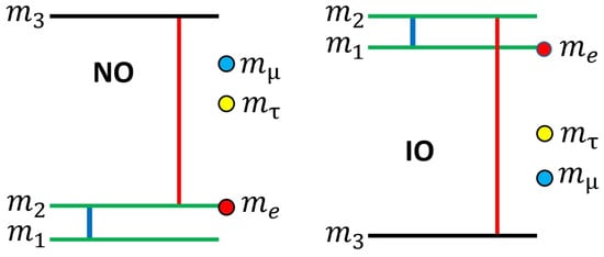
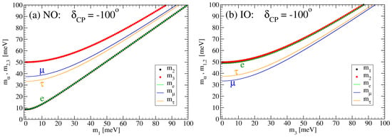
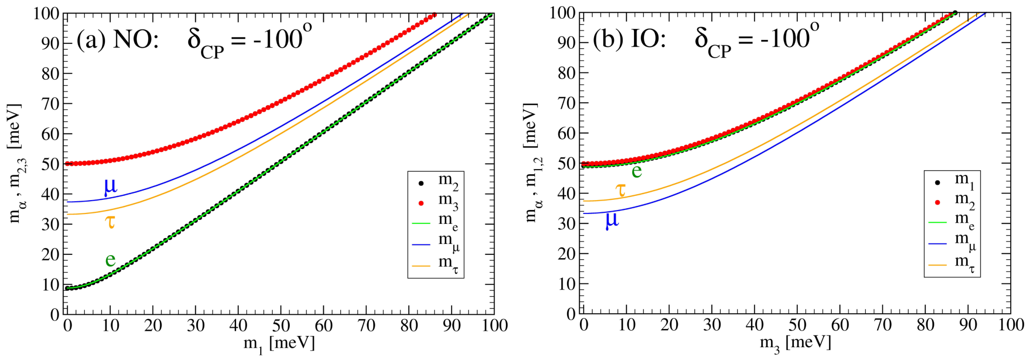
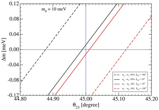
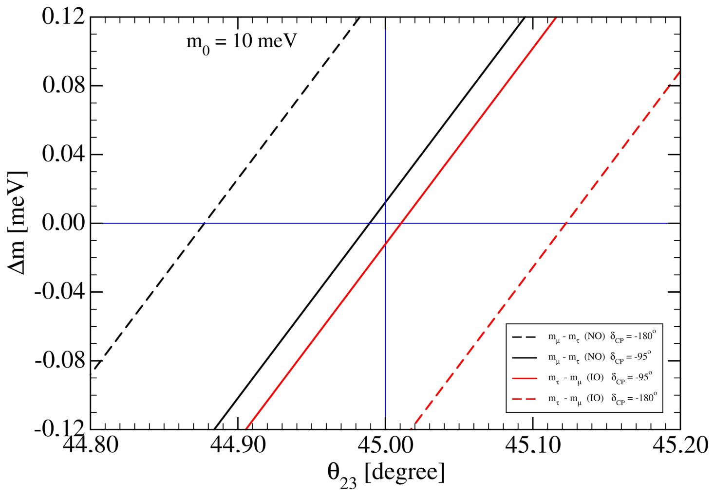
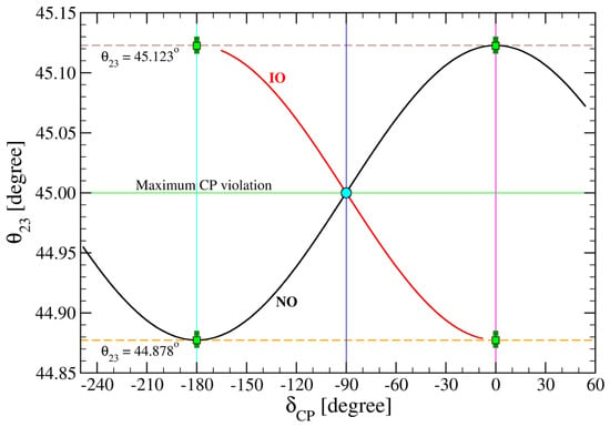
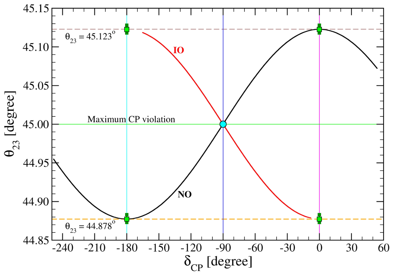
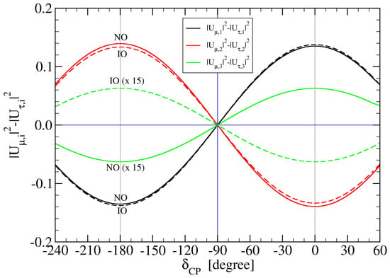
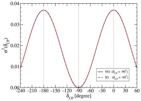
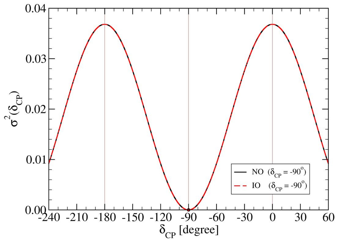
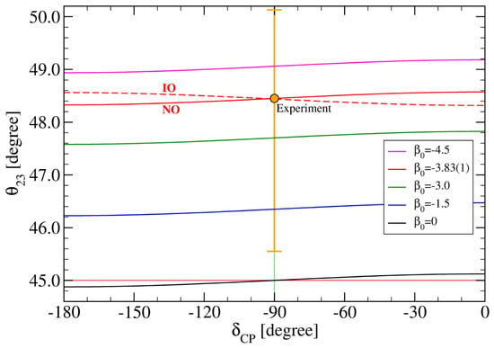
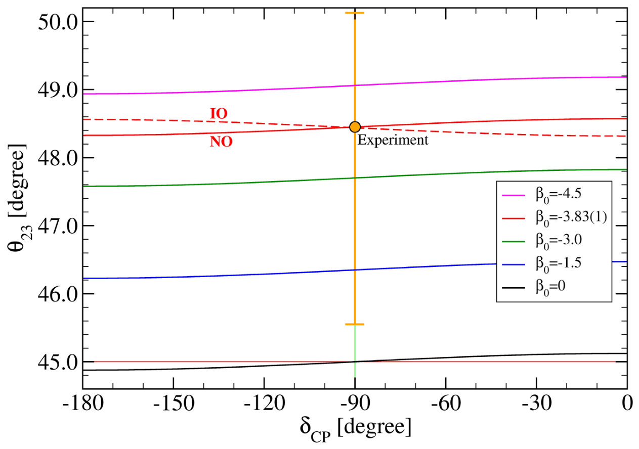
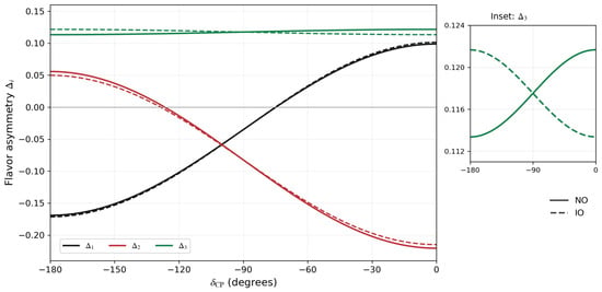
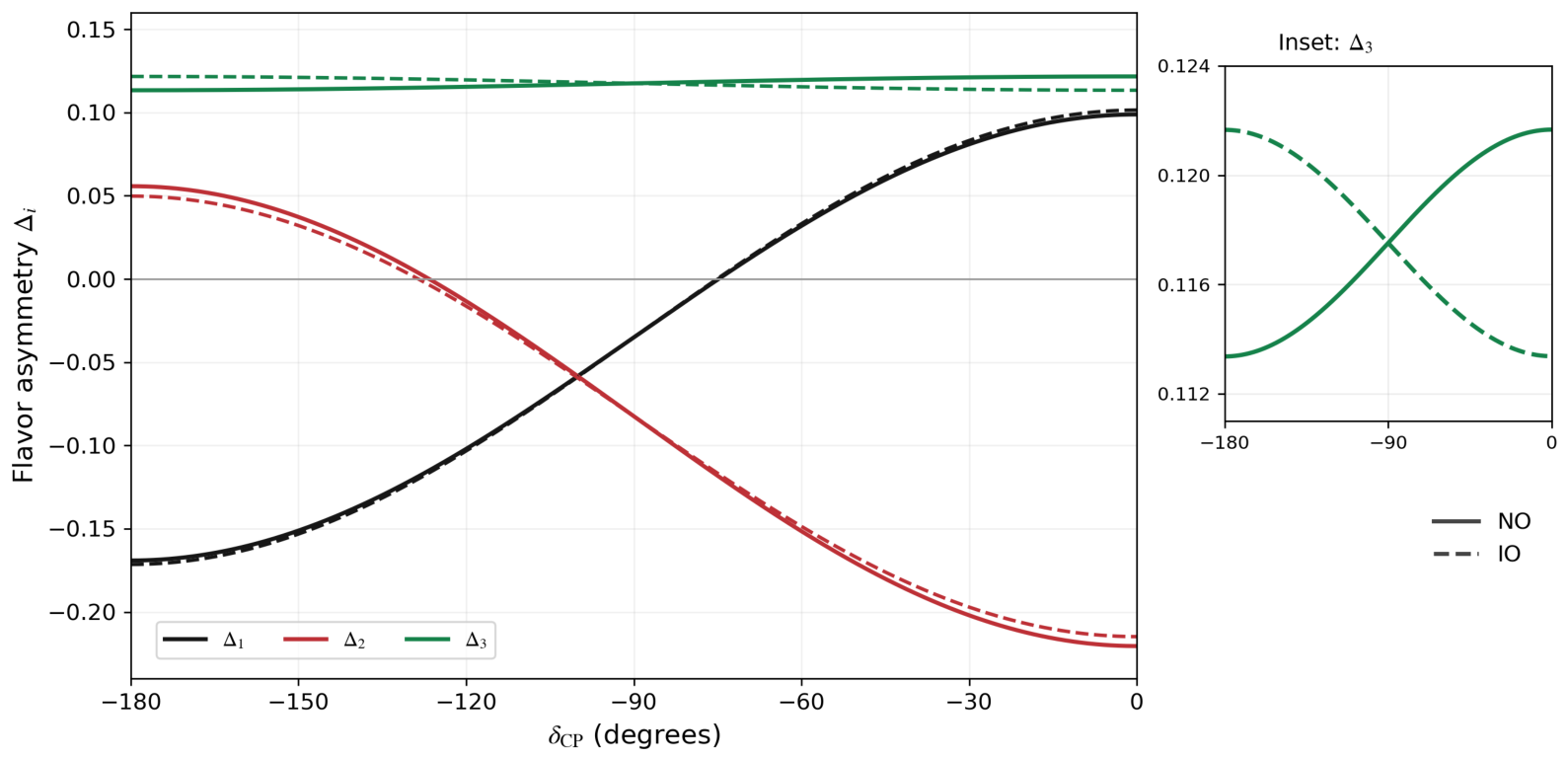
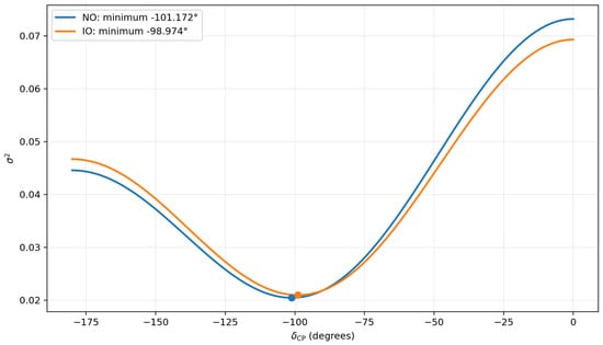
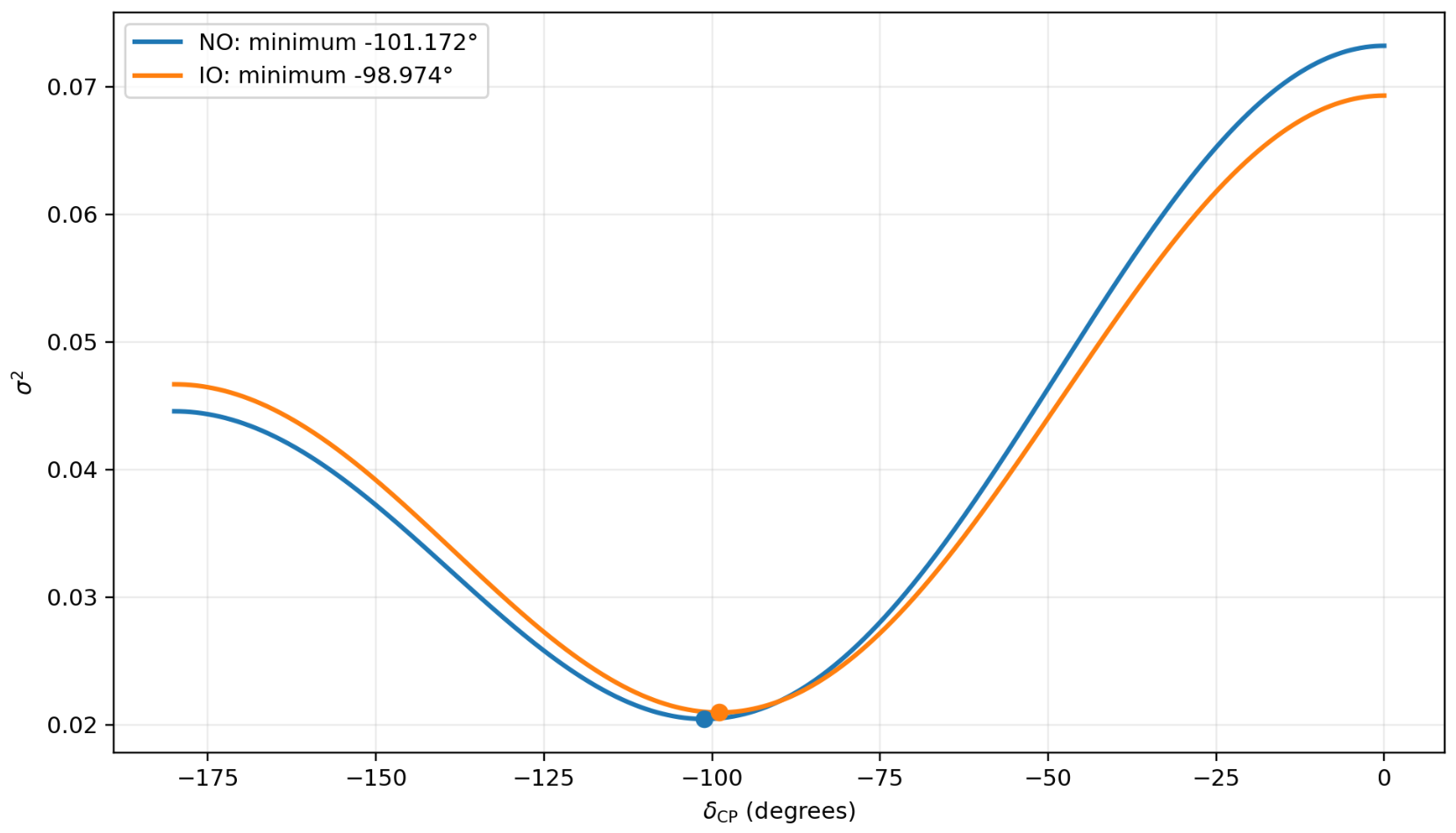
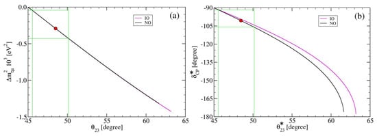
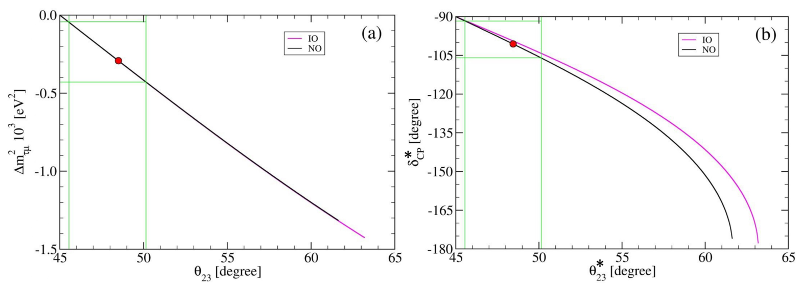
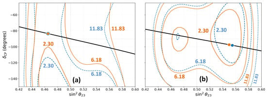
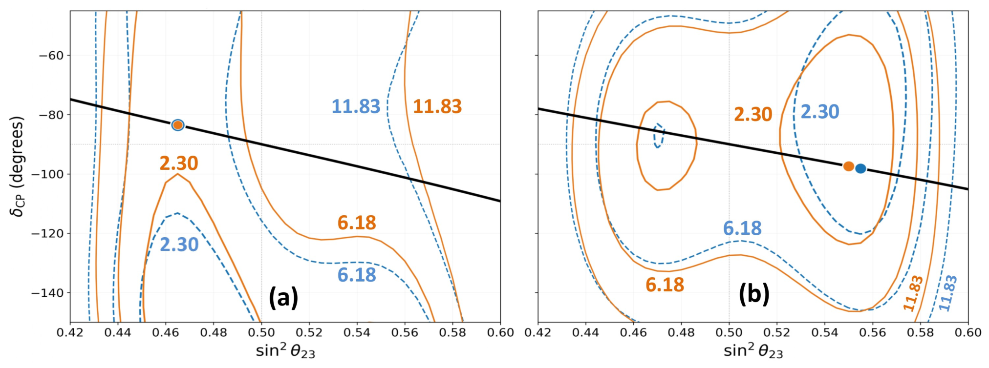

Disclaimer/Publisher’s Note: The statements, opinions and data contained in all publications are solely those of the individual author(s) and contributor(s) and not of MDPI and/or the editor(s). MDPI and/or the editor(s) disclaim responsibility for any injury to people or property resulting from any ideas, methods, instructions or products referred to in the content. |
© 2026 by the author. Licensee MDPI, Basel, Switzerland. This article is an open access article distributed under the terms and conditions of the Creative Commons Attribution (CC BY) license.