


Abstract
In this paper, we initiate the study of multivalued fixed point results in the framework of rectangular m-metric spaces. We establish fixed point theorems for Reich–Rus–Ćirić-type contractions and analyze two distinct cases based on the sum of the interpolative exponents: when the sum is less than one and when it is greater than one. Furthermore, by introducing the Hausdorff metric structure induced by rectangular m-metrics, our results generalize and extend various existing results in the literature. Illustrative examples are also provided to support and validate the obtained results.
Keywords:
interpolative Reich–Rus–Ćirić-type contractions; multivalued mappings; fixed point; rectangular m-metric (RMM) spaces MSC:
47H04; 47H10; 54H25; 54E50
1. Introduction
The fixed point theory has seen significant development across numerous branches after the introduction of Banach’s classical fixed point theorem in 1922 [1]. Subsequently, in 1968, Kannan [2] introduced a new class of contraction mappings, now known as Kannan contractions, and established an associated fixed point theorem. These pioneering results were later extended and generalized by Reich, Rus, and Ćirić.
Later, Karapınar [3] revisited Kannan’s contraction principle and introduced, for the first time, the notion of an interpolative Kannan-type contraction. In his work, the existence of fixed points for mappings satisfying this new contraction condition was also established. This contribution marked an important development in fixed point theory and stimulated further investigations into this class of contraction mappings. Motivated by Karapınar’s results, Gabba et al. [4] generalized the theory to the situation in which the sum of the interpolative parameters is strictly less than one. On the other hand, Errai et al. [5] examined the complementary case where this sum is greater than or equal to one. It is worth noting that all of these results were obtained in the setting of classical metric spaces.
Furthermore, Karapınar et al. [6] introduced the concept of interpolative Reich–Rus–Ćirić-type contractions and established several fixed point results for mappings of this type in the setting of partial metric spaces.
In a different direction, Özgür et al. [7] proposed a new extension of metric spaces, referred to as RMM spaces. In their work, it was shown that this class of spaces properly generalizes both partial metric spaces [8] and m-metric spaces [9]. For further developments and related contributions in fixed point theory connected to the present study, the reader is referred to [10,11,12,13,14,15,16,17,18,19] and the references therein.
Motivated by these developments, the present paper initiates a systematic investigation of fixed point results for multivalued interpolative Reich–Rus–Ćirić-type contractions in the framework of RMM spaces. We establish new fixed point theorems corresponding to different choices of interpolative exponents. The first section is devoted to preliminary notions and auxiliary results concerning RMM spaces and interpolative Reich–Rus–Ćirić-type contractions. In the subsequent section, we derive new fixed point results for such contractions under two distinct scenarios, namely, when the sum of the interpolative exponents is less than one and when it exceeds one. Each theoretical result is illustrated with an appropriate example.
2. Preliminaries
Definition 1
([9]). Let Γ be a nonempty set. A function
is called an -metric if following properties holds:
for all The pair is called -metric space.
Definition 2
([7]). Let Γ be a non-empty set, and let be a function. Suppose that for every , the following conditions hold:
where and and , then the pair is said to form a rectangular -metric space, abbreviated as an RMM space. This abbreviation will be used throughout the paper.
Definition 3
([7]). Let be a RMM space. Then, the following statements hold:
- A sequence in Γ converges to a point iff
- A sequence is called an -Cauchy sequence iff the following limits exist and are finite:
- The space is said to be -complete if every -Cauchy sequence in Γ converges to some , satisfying
Lemma 1
([7]). Let and be sequences in a RMM space such that and as . Then, the following limit holds:
Lemma 2
([7]). Let be a sequence in a RMM space that converges to as . Then, for every , the following limit holds:
Lemma 3
([7]). Let be a sequence in a RMM space . Suppose there exists a constant such that
then the following statements hold:
- ,
- ,
- ,
- the sequence is -Cauchy.
Theorem 1
([7]). Let be a complete RMM space, and let be a self-mapping. If such that
then admits a unique fixed point in Γ, satisfying .
Theorem 2
([7]). Suppose is a complete RMM space and is a self-mapping. If such that
then has a unique fixed point in Γ, with .
We now move our attention from single-valued mappings to set-valued mappings. To facilitate this transition, it is essential to introduce an appropriate notion of distance between sets. Such a concept is naturally derived by extending the idea of distance between individual points, subject to suitable constraints.
Let denote the family of all closed and bounded subsets of , and let represent the collection of all compact subsets of . After introducing the necessary preliminary notions, we can now define the Hausdorff metric for a given metric space.
Definition 4.
Let be a metric space. Define the function by where
 Equivalently,
 can be expressed as

whereEquivalently, can be expressed asWe now illustrate the computation of the distance between sets with a concrete example.
Example 1.
Let be equipped with the standard metric . Consider the subsets and  . We compute the Hausdorff distance between these subsets in , which is given as

. We compute the Hausdorff distance between these subsets in , which is given asIn parallel with the development of several generalized distance frameworks, such as partial metric spaces, -metric spaces, and their rectangular variants, researchers have also sought to generalize the classical Hausdorff metric, which quantifies the distance between subsets of a metric space. The primary objective of these extensions is to reformulate the Hausdorff construction so that it remains compatible with more general metric-type structures. Within this line of research, a significant advancement is the introduction of a Hausdorff distance induced by an -metric. This generalized Hausdorff distance provides an appropriate tool for studying set-valued mappings in -metric spaces. In particular, Patle et al. [20] proposed a Hausdorff-type metric adapted to the intrinsic properties of -metrics, thereby facilitating the extension of fixed point results to multivalued mappings in this broader setting. Such generalizations substantially enrich the applicability of metric fixed point theory.
Definition 5
([20]). Let Γ be a nonempty set equipped with an -metric. Denote by the collection of all nonempty, closed, and bounded subsets of Γ. For any  , we define the Hausdorff-type metric as
 where

, we define the Hausdorff-type metric aswhereLemma 4
([20]). Let  . Then the following statements hold:
- (i)
- ,
- (ii)
- For any
 ,

Proposition 1
([20]). Let  . The following properties hold:
- (i)
- .
- (ii)
 .
- (iii)
- The following inequality is satisfied:

Building on the preceding proposition, the function
is referred to as the -Pompeiu–Hausdorff metric.
The following definitions and topological concepts are adapted from [20].
Lemma 5
([20]). Let ℵ be a non-empty subset of an -metric space , and define
Then, if and only if
Lemma 6
([20]). Let ℵ and  be elements in , and let . Then for each element , there exists an element
 such that

be elements in , and let . Then for each element , there exists an element such that3. -Pompeiu–Hausdorff-Type Metric
In this section, we introduce a generalized Hausdorff-type distance defined on RMM spaces. This distance provides a natural way to measure the separation between two nonempty subsets when the underlying space is an RMM space, where the classical triangle inequality is replaced by a rectangular-type condition.
The main purpose of this construction is to extend the classical Hausdorff metric so that it is compatible with generalized metric frameworks, particularly those arising in the study of multivalued mappings. By formulating the Hausdorff distance within the setting of RMM spaces, we obtain a useful analytical tool for establishing fixed point results for multivalued mappings in this more general context.
The formal definition of this distance, together with its basic properties, is given below.
Definition 6.
Let be collection of nonempty, bounded, and closed subsets of a RMM space . For any  , we define the Hausdorff-type -distance between ℵ and as
 where

, we define the Hausdorff-type -distance between ℵ and aswhereWe now introduce the concept of boundedness in the context of RMM spaces.
Definition 7.
A subset U of a RMM space is said to be bounded if, for each , there exist an element and a non-negative number such that
where denotes the ball in the RMM, defined by
Let denote the closure of a set ℵ in the RMM space . Recall that a set ℵ is closed if and only if it coincides with its closure, that is, .
Lemma 7.
Let ℵ be a non-empty subset of the RMM space . Then, for any ,
Proof.
Let ℑ be an arbitrary point in the closure of ℵ. By the definition of closure, we have:
Since the above inequality holds for every , taking the infimum over all yields:
□
Note that the proof presented above closely resembles that of Lemma 6 in [20], as it does not rely on the rectangular inequality.
Proposition 2.
Let  . Then, the following statements hold:
- (a)
- .
- (b)
- The following inequality is satisfied:

Proof.
(a) Since , it follows that . By Lemma 7, we have
Consequently,
- For any
 , and , the following inequality holds as a consequence of :
By rearranging the preceding inequality, we obtain
Since ℑ is chosen arbitrarily from , it follows that  Noting that
 and applying the symmetry property , which gives , the above inequality can be expressed equivalently as
 Since is an arbitrary element of , it follows that
 Furthermore, noting that , we obtain
 Since is an arbitrary element of F, it follows that:
 Alternatively, we have
 Taking the supremum over all , we obtain
 Observing that
we thus arrive at the following inequality:

, it follows that Noting that and applying the symmetry property , which gives , the above inequality can be expressed equivalently as Since is an arbitrary element of , it follows that Furthermore, noting that , we obtain Since is an arbitrary element of F, it follows that: Alternatively, we have Taking the supremum over all , we obtain Observing that □
Proposition 3.
Let  . Then the following statements hold:
- .
 .
- The following inequality holds:

Proof. 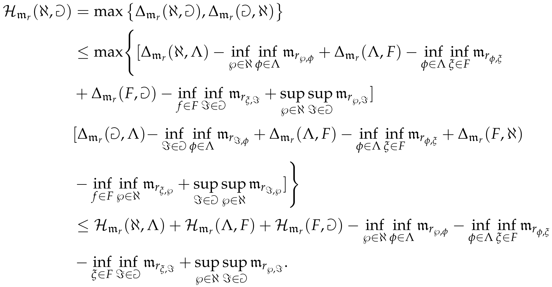 □
(i) By applying Definition 6 together with part of Proposition 2, we obtain
- This result follows directly from property of Definition 2.
- Using part of Proposition 2, we can express
□In view of Proposition 3, is said to be an -Pompeiu–Hausdorff-type metric induced by RMM.
4. Multivalued -Interpolative Contractions
This section focuses on establishing fixed point result for a class of multivalued mappings known as multivalued -interpolative Reich–Rus–Ćirić-type contractions. These mappings are considered within the framework of RMM spaces and are defined in terms of a Hausdorff-type distance derived from the RMM. By introducing the parameters with the condition The primary aim is to establish conditions under which such mappings possess fixed points. The precise definition of these multivalued contractions is stated below.
Definition 8.
Let be a RMM space. A mapping is called a multivalued -interpolative Reich–Rus–Ćirić-type contraction if there exist constants satisfying , such that
for all , with and .
Lemma 8.
Let  and let . For each element , there exists an element
 such that

and let . For each element , there exists an element such thatProof.
Suppose, on the contrary, that there exists some such that Then we have
 which implies
 Observe that
 Since
 , it follows that , which contradicts our assumption that . Therefore, our initial supposition is false, and we conclude that for every , there exists such that

Then we have
which implies Observe that Since , it follows that , which contradicts our assumption that . Therefore, our initial supposition is false, and we conclude that for every , there exists such that□
Theorem 3.
Let be a complete RMM space. Suppose that is a multivalued -interpolative Reich–Rus–Ćirić contraction. Then possesses at least one fixed point in Γ.
Proof.
Let us choose and . Take any element and let . Since , it follows from Lemma 8 that there exists an element satisfying
Furthermore, applying inequality (5), we obtain
By combining the inequalities (6) and (7), we derive
Furthermore, since for every , the above inequality can be rewritten as
Assuming , this inequality can be further simplified to yield
Since and , it follows that . Consequently, we obtain
Applying Lemma 8 once more, there exists such that
Furthermore, from inequality (5), and by following a similar argument as above, we get
Proceeding in the same manner, we define a sequence such that, for every , it satisfies:
Since for all n, it follows from Lemma 3 that the sequence is -Cauchy. Given that is complete, the sequence converges to some element, denoted by . Therefore, by the definition of convergence, we have:
Applying Lemma 3 again, we obtain , which leads to:
Applying the relation (5) to the equation above, we obtain
Furthermore, since , it follows that
Consequently, from (15), we deduce
Now, for any , we have that is, By taking the limit on both sides of the inequality and employing inequality (16), we obtain
Moreover, for and , there exists such that
Applying condition () from Definition 2, we then deduce that:
By taking the limit in the above inequality and employing the relations (13)–(15) and (17), together with the facts that
we obtain
Noting that
it follows immediately that Thus or It follows that
By applying inequalities (18) and (19), we obtain
Consequently, Lemma 7 implies that
which shows that is a fixed point of the mapping within the set . □
Remark 1.
In [6], the result was established for single-valued mappings on partial metric spaces, assuming that the sum of the interpolative exponents is less than one for interpolative Reich–Rus–Ćirić-type contractions. In contrast, Theorem 3 extends this concept to multivalued mappings in RMM spaces.
5. Multivalued -Interpolative Contractions
In this section, we investigate a fixed point result for a new class of multivalued mappings, which we refer to as multivalued -interpolative Reich–Rus–Ćirić-type contractions. These mappings are studied within the framework of RMM spaces, using a Hausdorff-type distance suitably adapted to their multivalued nature. Unlike the results in the previous section, the interpolative parameters and here satisfy the condition . The formal definition of these mappings is presented below.
Definition 9.
Let be a RMM space. A mapping is called a multivalued -interpolative Reich–Rus–Ćirić-type contraction if there exist constants with such that
for all satisfying and .
Theorem 4.
Let be a complete RMM space, and let be a multivalued mapping satisfying -interpolative Reich–Rus–Ćirić contraction. Suppose there exists a point such that
Then admits at least one fixed point in Γ.
Proof.
Let us choose and , so that and . Consider a point satisfying for every . Since , Lemma 8 ensures the existence of a point such that
Applying inequality (20) to the term , we obtain:
Utilizing inequalities (21) and (22), along with the observation that for every , we obtain:
Simplifying the above inequality yield
Since and , it follows that
Moreover, as , we have
Consequently, we obtain the following estimate:
Furthermore, by Lemma 8, for any , there exists such that
Applying inequality (20) to and then by following the similar argument as above, we get
Combining (23) and (25), it follows that
By applying this process iteratively, we derive the general inequality
Using the inequalities obtained from previous iterations, we can further conclude that
Since , it follows that for all positive integers n. Finally, by substituting n with in (27), we obtain the subsequent inequality.
Observe that , which implies since . Furthermore, as established above, we have , which yields
Consequently, inequality (29) can be rewritten as
Since , it follows that . Therefore, by Lemma 3, the sequence is -Cauchy. As the space is complete, the sequence converges to some limit, denoted by , in . Thus, by following a procedure similar to that used in Theorem 3, we obtain the following relation:
Hence, by invoking Lemma 7, we conclude that
which shows that is a fixed point of in . □
Remark 2.
The results in [21] concern single-valued interpolative Reich–Rus–Ćirić-type contractions defined on RMM spaces, covering both cases when the sum of the interpolative exponents is less than one and when it is greater than one. Our results, Theorems 3 and 4, extend this concept to the setting of multivalued mappings.
6. Examples
In this section, we furnish examples to substantiate the theoretical results established earlier. These examples serve to illustrate the effectiveness and stability of the proposed fixed point theorems under diverse assumptions. Furthermore, explicit computational demonstrations are included to provide a clearer insight into the behavior of the associated multivalued contraction mappings.
Example 2.
Let us consider the set , equipped with a RMM defined by
Define the mapping as follows:
To verify our results, we examine all possible cases while choosing the constants , , and .
- Case (i).
- Let . Then, we have
On the other hand, we have
Substituting the above estimate into inequality (5) leads to
A valid range for the parameter ℘ satisfying this inequality is
Now, in the following cases, we verify the validity of the inequality (5) for .
- Case (ii).
- For and ,
On the other hand,
Substituting the previously obtained expressions into inequality (5) yields
This inequality holds for all . Next, if we interchange the roles of and ϱ so that and , we obtain
Substituting these expressions back into inequality (5) leads to
This inequality is satisfied for all
- Case (iii).
- Let . Then, we have
Further,
Substituting the expressions derived above into inequality (5) gives
A subset of the solutions to this inequality is given by the interval . Hence, this interval lies entirely within the set of all solutions identified above. Therefore, this example confirms the validity of our fixed point Theorem 3 for , with
Example 3.
To verify Theorem 4, we consider the set equipped with the metric
Define the mapping by
We select the parameters and , which satisfy .
- Case (i).
- Let . Then,
On the other hand,
Substituting the previously obtained expressions into inequality (20) gives
This inequality holds for all . Next, we examine the validity of inequality (20) for other possible scenarios when .
- Case (ii).
- Consider and . Then
On the other hand,
Substituting these derived expressions into inequality (20) yields
It can be verified that this inequality is satisfied for all . Furthermore, if we exchange the roles of and ϱ, taking and , we obtain
Substituting the expressions obtained above into inequality (20) yields
It can be verified that this inequality is satisfied for all .
- Case (iii).
- Let . Then
On the other hand,
Substituting the previously derived expressions into inequality (20) leads to
It can be verified that this inequality holds for all . Therefore, this example confirms the validity of Theorem 4 for , with
7. Conclusions
This paper establishes new multivalued fixed point results in the setting of RMM spaces by employing Reich–Rus–Ćirić-type contractive conditions. The analysis distinguishes two cases based on the sum of the interpolative exponents, allowing the obtained results to cover a wider class of multivalued contractions. By using the Hausdorff metric induced by rectangular -metrics, our theorems extend several existing fixed point results in generalized metric spaces. The examples provided confirm the applicability of the theoretical results.
Author Contributions
Conceptualization, S.H.K. and A.R.; formal analysis, M.Z. and A.R.; funding acquisition, S.H.K.; investigation, M.Z. and A.R.; methodology, S.H.K. and A.R.; supervision, S.H.K.; writing—original draft, M.Z. and A.R.; writing—review and editing, S.H.K. and A.R. All authors have read and agreed to the published version of the manuscript.
Funding
The funding is arranged by Safeer Hussain Khan.
Data Availability Statement
The data presented in this study are available on request from the corresponding author.
Conflicts of Interest
The authors declare no conflicts of interest.
References
- Banach, S. Sur les opérations dans les ensembles abstraits et leur application aux équations intégrales. Fund. Math 1922, 3, 133–181. [Google Scholar] [CrossRef] [Scilit]
- Kannan, R. Some results on fixed points. Bull. Cal. Math. Soc. 1968, 60, 71–76. [Google Scholar]
- Karapinar, E. Revisiting the Kannan type contractions via interpolation. Adv. Theory Nonlinear Anal. Its Appl. 2018, 2, 85–87. [Google Scholar] [CrossRef] [Scilit]
- Gaba, Y.U.; Aydi, H.; Mlaiki, N. (ρ, n, μ)-Interpolative Kannan Contractions I. Axioms 2021, 10, 212. [Google Scholar] [CrossRef] [Scilit]
- Errai, Y.; Marhrani, E.M.; Aamri, M. Some remarks on fixed point theorems for interpolative Kannan contraction. J. Funct. Spaces 2020, 2020, 2075920. [Google Scholar] [CrossRef] [Scilit]
- Karapinar, E.; Agarwal, R.; Aydi, H. Interpolative Reich–Rus–Ćirić type contractions on partial metric spaces. Mathematics 2018, 6, 256. [Google Scholar] [CrossRef] [Scilit]
- Özgür, N.Y.; Mlaiki, N.; Taş, N.; Souayah, N. A new generalization of metric spaces: Rectangular M-metric spaces. Math. Sci. 2018, 12, 223–233. [Google Scholar] [CrossRef] [Scilit]
- Matthews, S.G. Partial metric spaces. Am. Math. Mon. 1992, 116, 708–718. [Google Scholar]
- Asadi, M.; Karapınar, E.; Salimi, P. New extension of p-metric spaces with some fixed-point results on M-metric spaces. J. Inequalities Appl. 2014, 2014, 1–9. [Google Scholar] [CrossRef] [Scilit]
- Ćirić, L.B. A generalization of Banach’s contraction principle. Proc. Am. Math. Soc. 1974, 45, 267–273. [Google Scholar] [CrossRef] [Scilit]
- Aydi, H.; Chen, C.M.; Karapınar, E. Interpolative Ćirić-Reich-Rus type contractions via the Branciari distance. Mathematics 2019, 7, 84. [Google Scholar] [CrossRef] [Scilit]
- Branciari, A. A fixed point theorem of Banach-Caccioppoli type on a class of generalized metric spaces. Publ. Math. Debr. 2000, 57, 31–37. [Google Scholar] [CrossRef] [Scilit]
- Brzdęk, J.; Karapınar, E.; Petruşel, A. A fixed point theorem and the Ulam stability in generalized dq-metric spaces. J. Math. Anal. Appl. 2018, 467, 501–520. [Google Scholar] [CrossRef] [Scilit]
- George, R.; Radenovic, S.; Reshma, K.P.; Shukla, S. Rectangular b-metric space and contraction principles. J. Nonlinear Sci. Appl. 2015, 8, 1005–1013. [Google Scholar] [CrossRef] [Scilit]
- Mebarki, K.; Boudaoui, A.; Belhenniche, A.; Bota, M.F. Fixed-Point Theorems for Covariant and Contravariant Multivalued Mappings in Bipolar b-Metric Spaces. Mathematics 2025, 13, 2983. [Google Scholar] [CrossRef] [Scilit]
- Nadler, S.B., Jr. Multi-valued contraction mappings. Pac. J. Math. 1969, 30, 475–488. [Google Scholar] [CrossRef] [Scilit]
- Raza, A.; Khan, S.H. Interpolative contractive results for multivalued mappings over m-metric spaces with an application in homotopy. Filomat 2024, 38, 3547–3562. [Google Scholar] [CrossRef] [Scilit]
- Reich, S. Some remarks concerning contraction mappings. Can. Math. Bull. 1971, 14, 121–124. [Google Scholar] [CrossRef] [Scilit]
- Shukla, S. Partial rectangular metric spaces and fixed point theorems. Sci. World J. 2014, 2014, 756298. [Google Scholar] [CrossRef] [Scilit]
- Patle, P.R.; Kumar Patel, D.; Aydi, H.; Gopal, D.; Mlaiki, N. Nadler and Kannan type set valued mappings in M-metric spaces and an application. Mathematics 2019, 7, 373. [Google Scholar] [CrossRef] [Scilit]
- Zahid, M.; Raza, A.; Khan, S.H. Some Innovative Results for Interpolative Reich–Rus–Ćirić-Type Contractions in Rectangular m-Metric Spaces. Axioms 2024, 13, 829. [Google Scholar] [CrossRef] [Scilit]
Disclaimer/Publisher’s Note: The statements, opinions and data contained in all publications are solely those of the individual author(s) and contributor(s) and not of MDPI and/or the editor(s). MDPI and/or the editor(s) disclaim responsibility for any injury to people or property resulting from any ideas, methods, instructions or products referred to in the content. |
© 2026 by the authors. Licensee MDPI, Basel, Switzerland. This article is an open access article distributed under the terms and conditions of the Creative Commons Attribution (CC BY) license.