Radical Numerical Semigroups

Abstract

This work contributes to the study of radical numerical semigroups. If $n\in \mathbb{Z}$ where $n\ge 2$, then the product of all its prime positive divisors is called the radical of n. It is denoted by $\mathrm{r}\left(n\right)$. A radical numerical semigroup is a numerical semigroup S such that $s+\mathrm{r}\left(s\right)\in S$ for every $s\in S\backslash \left\{0\right\}$. We present three algorithms that will help us understand the structure of radical semigroups. These algorithms allow us to calculate all radical numerical semigroups with a fixed genus, with a fixed Frobenius number, as well as with a fixed multiplicity. Furthermore, given X, a set of positive integers such that $gcd\left(X\right)=1$, we will prove the existence of the smallest radical semigroup containing X. We will also present an algorithm to obtain it.

1. Introduction

Let $\mathbb{Z}=\{0,1,-1,2,-2,\dots \}$ be the set of integers and $\mathbb{N}=\{x\in \mathbb{Z}\mid x\ge 0\}$. A subset M of $\mathbb{N}$ is a submonoid of $(\mathbb{N},+)$ if $a+b\in M$ for all $a,b\in M$ and $0\in M$. We will say that a submonoid S of $(\mathbb{N},+)$ is a numerical semigroup if $\mathbb{N}\setminus S=\{x\in \mathbb{N}\mid x\notin S\}$ is a finite set.

Given S, a numerical semigroup, let us consider the following notable elements of S: $\mathrm{m}\left(S\right)=min(S\setminus \{0\left\}\right)$, $\mathrm{F}\left(S\right)=max\{z\in \mathbb{Z}\mid z\notin S\}$ and $\mathrm{g}\left(S\right)=♯(\mathbb{N}\setminus S)$ (where $♯X$ denotes the cardinality of a set X). These are three important invariants, which we will call multiplicity, the Frobenius number and the genus of S, respectively.

Let A be a non-empty subset of $\mathbb{N}$. Denote by $⟨A⟩$ the submonoid of $(\mathbb{N},+)$ generated by A. That is

$$⟨A⟩=\{{\lambda }_1{a}_1+\cdots +{\lambda }_r{a}_r\mid r\in \mathbb{N}\setminus \left\{0\right\},\{a_1,\dots ,a_r\}\subseteq A \mathrm{and}\{{\lambda }_1,\dots ,{\lambda }_r\}\subseteq \mathbb{N}\}.$$

By virtue of ([1], Lema 2.1), the necessary and sufficient condition for $⟨A⟩$ to be a numerical semigroup is $gcd\left(A\right)=1$.

We will say that a non-empty subset A of $\mathbb{N}$ constitutes a system of generators of a submonoid M of $\mathbb{N}$ if $M=⟨A⟩$. When this set is minimal with respect to inclusion order, then A is a minimal system of generators of M. In ([1], Corollary 2.8), it is proven that every submonoid of $(\mathbb{N},+)$ has a unique minimal system of generators, which is finite. The minimal system of generators of M will be denoted by $\mathrm{msg}\left(M\right)$. The cardinality of this system defines the embedding dimension of M and will be denoted by $\mathrm{e}\left(M\right)$.

There is a close relationship between numerical semigroups and Diophantine equations, since historically numerical semigroups arose from the study of the solutions of Diophantine equations.

The study of numerical semigroups is equivalent to the study of non-negative integer solutions of a linear equation with coefficients in $\mathbb{N}$. For this reason, it is a classic problem, and there is a large list of works dedicated to its study (see, for instance, [2,3,4,5,6,7,8,9]).

The reader unfamiliar with the study of numerical semigroups may find the notation multiplicity, embedding dimension, genus, … somewhat surprising.

We will say in this regard that in the literature there is a long list of publications dedicated to the study of analytically irreducible one-dimensional local domains via their semigroup of values, which turns out to be a numerical semigroup (see [10,11,12,13,14,15,16,17]). All these invariants introduced above have their interpretation in this context, hence their names. In this sense [10], it is a good dictionary for translating the results of numerical semigroup theory into ring theory.

The Frobenius problem for numerical semigroups consists of calculating invariants such as genus and Frobenius number based solely on the minimal generators of the semigroup (see [18]). Historically, the two-embedding dimension case was solved by Sylvester [19]; however, finding a general solution for embedding dimension greater than or equal to three remains one of the outstanding challenges in the theory today. Despite this, current research has led to solutions for a wide variety of special families of numerical semigroups (see, for instance, [2,4,5,6,7,17]).

The relationship between the Frobenius number, the genus and the embedding dimension of a numerical semigroup is also a research problem in the theory of numerical semigroups. Indeed, if S is a numerical semigroup, then A.S. Wilf conjectures in [20] that $\mathrm{e}\left(S\right)\mathrm{g}\left(S\right)\le \left(\mathrm{e}\right(S)-1)\left(\mathrm{F}\right(S)+1)$. Currently unsolved, this problem stands as a cornerstone of numerical semigroup theory. However, the conjecture has been validated for numerous specific classes of semigroups (see, for example, [21,22,23,24,25]).

If $g\in \mathbb{N}$, then denote by $\mathrm{S}\left(g\right)=\{S\mid S\mathrm{is} \mathrm{a} \mathrm{numerical} \mathrm{semigroup} \mathrm{and} \mathrm{g}(S)=g\}$. This set has been widely considered in the literature (see [26,27,28,29,30]). Many of these works are motivated by the conjecture presented in [27], in which it is asserted that the sequence ${\{\#\mathrm{S}\left(g\right)\}}_{g\in \mathbb{N}}$ is increasing and has a behavior similar to the Fibonacci sequence. In [31] it is shown that ${\displaystyle \underset{g\to \infty }{lim}\frac{\#\mathrm{S}\left(g\right)}{\#\mathrm{S}(g-1)}}$ is the golden number, and therefore the asymptotic behavior of the sequence ${\{\#\mathrm{S}\left(g\right)\}}_{g\in \mathbb{N}}$ is similar to the behavior of the Fibonacci sequence. However, it is currently an open problem to demonstrate that $\#\mathrm{S}(g-1)\le \#\mathrm{S}\left(g\right)$ for every $g\in \mathbb{N}\setminus \left\{0\right\}$.

If $n\in \mathbb{N}\setminus \{0,1\}$, then the radical of n, denoted by $\mathrm{r}\left(n\right)$, is the product of all positive prime numbers that divide n. Thus, if $n=P_1^{{\alpha }_1}·\dots$$·P_k^{{\alpha }_k}$ is the expression of an integer n greater than or equal to two, as a product of prime numbers, then $\mathrm{r}\left(n\right)=P_1·\dots$$·P_k$. This concept is used in different parts of Number Theory, such as in the formulation of the abc conjecture, also known as the Oesterlé–Masser conjecture (see [32,33,34,35]). This conjecture is considered the most important unsolved problem in Diophantine analysis.

Given S a numerical semigroup, if $s+\mathrm{r}\left(s\right)\in S$ for all $s\in S\setminus \left\{0\right\}$, then we say that S is radical. The main purpose of this work will be to explore this kind of numerical semigroups.

Denote by $\mathcal{R}=\{S\mid S\mathrm{is} \mathrm{a} \mathrm{radical} \mathrm{numerical} \mathrm{semigroup}\}$. We begin Section 2 by showing that $\mathcal{R}$ is a Frobenius variety with infinite cardinality. This fact, together with the results of [36], allows us to construct a tree whose set of vertices is $\mathcal{R}$. As an application, we will present an algorithm that enables us to calculate all radical numerical semigroups with a given genus.

If $X\subseteq \mathbb{N}$, then we denote by $\mathcal{R}\left[X\right]$ the intersection of all elements of $\mathcal{R}$ that contain X. In Section 3, we will see that $\mathcal{R}=\left\{\mathcal{R}\right[X]\mid X\subseteq \mathbb{N}\setminus \{0\},X \mathrm{finite} \mathrm{and} gcd(X)=1\}$. Moreover, we will show an algorithm that computes $\mathcal{R}\left[X\right]$ from a finite subset X of $\mathbb{N}\setminus \left\{0\right\}$ such that $gcd\left(X\right)=1$.

For any positive integer $\mathrm{F}$, let $\mathcal{R}\left(F\right)=\{S\in \mathcal{R}\mid \mathrm{F}(S)=F\}$. At the beginning of Section 4, we show that $\mathcal{R}\left(F\right)$ constitutes a covariety. This property, combined with the findings in [37], enables the construction of a tree rooted whose set of vertices is $\mathcal{R}\left(F\right)$. Consequently, we designed an algorithm to compute all the elements of $\mathcal{R}\left(F\right)$.

Let $m\in \mathbb{N}\setminus \{0,1\}$. We define ${\mathcal{R}}_m$ as the set of elements in $\mathcal{R}$ with multiplicity m. After proving in Section 5 that ${\mathcal{R}}_m$ is an infinite Frobenius pseudo-variety, we apply the results from [38] to organize ${\mathcal{R}}_m$ into a tree structure. Finally, we propose an algorithm to find all semigroups in ${\mathcal{R}}_m$ with a given genus $\mathrm{g}$.

In this paper, all the algorithms presented are illustrated with examples in order to demonstrate how they work as well as to facilitate their understanding. Furthermore, they can be implemented using the numerical SGP package in the GAP System (see [39,40]).

2. The Tree of Radical Numerical Semigroups

We say that a non-empty family $\mathcal{V}$ of numerical semigroups is a Frobenius variety if it verifies the following:

• If $\{S_1,S_2\}\subseteq \mathcal{V}$, then $S_1\cap S_2\in \mathcal{V}$.
• If $T\in \mathcal{V}$ and $T\ne \mathbb{N}$, then $T\cup \left\{\mathrm{F}\right(T\left)\right\}\in \mathcal{V}$.

Our first aim in this section will be to prove that $\mathcal{R}=\{S\mid S\mathrm{is} \mathrm{a} \mathrm{radical} \mathrm{numerical} \mathrm{semigroup}\}$ is a Frobenius variety. Note that $\{0,m,\to \}\in \mathcal{R}$, where the symbol → means that every integer greater than m belongs to the set, for all $m\in \mathbb{N}$. Consequently, $\mathcal{R}$ is a set with infinite cardinality.

It is clear that $\mathrm{F}\left(\mathbb{N}\right)=-1$ and $\mathrm{F}\left(S\right)\in \mathbb{N}\setminus \left\{0\right\}$ for all numerical semigroup S such that $S\ne \mathbb{N}$.

The following result has an easy proof:

Lemma 1.

The following is verified:

1. 

Let S be a numerical semigroup such that $S\ne \mathbb{N}$. Then $S\cup \left\{\mathrm{F}\right(S\left)\right\}$ is also a numerical semigroup.

2. 

If $S_1$ and $S_2$ are numerical semigroups, then $S_1\cap S_2$ is also a numerical semigroup. Moreover, $\mathrm{F}(S_1\cap S_2)=max\{\mathrm{F}\left(S_1\right),\mathrm{F}\left(S_2\right)\}$ and $\mathrm{m}(S_1\cap S_2)\ge max\{\mathrm{m}\left(S_1\right),\mathrm{m}\left(S_2\right)\}$.

Proposition 1.

$\mathcal{R}$ is a Frobenius variety.

Proof. 

As $\mathbb{N}\in \mathcal{R}$, then $\mathcal{R}\ne \varnothing$. If $\{S,T\}\subseteq \mathcal{R}$, then by Lemma 1, we know that $S\cap T$ is a numerical semigroup. If $x\in (S\cap T)\setminus \left\{0\right\}$, then $x\in S\setminus \left\{0\right\}$ and $x\in T\setminus \left\{0\right\}$. Thus, $x+\mathrm{r}\left(x\right)\in S\cap T$ and so $S\cap T\in \mathcal{R}$. Finally, if $S\in \mathcal{R}$ and $S\ne \mathbb{N}$, then by Lemma 1, we have that $S\cup \left\{\mathrm{F}\right(S\left)\right\}$ is a numerical semigroup. If $x\in (S\cup \{F\left(S\right)\left\}\right)\setminus \left\{0\right\}$, then we consider the following two cases:

• If $x\in S$, then $x+\mathrm{r}\left(x\right)\in S\subseteq S\cup \left\{\mathrm{F}\right(S\left)\right\}$.
• If $x=\mathrm{F}\left(S\right)$, then $x+\mathrm{r}\left(x\right)>\mathrm{F}\left(S\right)$, and so $x+\mathrm{r}\left(x\right)\in S\cup \left\{\mathrm{F}\right(S\left)\right\}$.

   □

A graph G is defined as a pair $(V,E)$ where V is a non-empty set and E is a subset of $\left\{\right(u,v)\in V\times V\mid u\ne v\}$. We will call the elements of V and E vertices and edges of the graph G, respectively.

A path of length n, connecting the vertices u and v of G, is a sequence of different edges of the form $(v_0,v_1),(v_1,v_2),\dots ,(v_{n-1},v_n)$ such that $v_0=u$ and $v_n=v$.

We will say that a graph G is a tree if there exists a vertex a (known as the root of G) such that for any other vertex v of G there exists a unique path connecting v and a. If $(u,v)$ is an edge of the tree G, we say that u is a child of v.

Consider the graph $\mathrm{G}\left(\mathcal{R}\right)$, defined in the following way: The set of vertices is $\mathcal{R}$ and $(S,T)\in \mathcal{R}\times \mathcal{R}$ is an edge if and only if $T=S\cup \left\{\mathrm{F}\right(S\left)\right\}$.

By Proposition 1 and ([36], Theorem 27), the following result is obtained. In it we can find a description of the children of the vertices in the tree $\mathrm{G}\left(\mathcal{R}\right)$.

Theorem 1.

$\mathrm{G}\left(\mathcal{R}\right)$ is a tree rooted at $\mathbb{N}$. In addition, the set formed by the children of a vertex S of $\mathrm{G}\left(\mathcal{R}\right)$ is $\{S\setminus \{x\}\mid x\in \mathrm{msg}(S),x>\mathrm{F}(S) and S\setminus \{x\}\in \mathcal{R}\}$.

The next result can be consulted in ([1], Lemma 2.3).

Lemma 2.

Let S be a numerical semigroup and $x\in S$. Then, $S\setminus \left\{x\right\}$ is a numerical semigroup if and only if $x\in \mathrm{msg}\left(S\right)$.

Proposition 2.

Let $S\in \mathcal{R}$ and $x\in \mathrm{msg}\left(S\right)$. Then, $S\setminus \left\{x\right\}\in \mathcal{R}$ if and only if $s+\mathrm{r}\left(s\right)\ne x$ for all $s\in S$ such that ${\displaystyle \frac{x}{2}}\le s<x$.

Proof. (Necessity).

If $s\in S$ and ${\displaystyle \frac{x}{2}}\le s<x$, then $s\in S\setminus \{0,x\}$. As $S\setminus \left\{x\right\}\in \mathcal{R}$, then $s+\mathrm{r}\left(s\right)\in S\setminus \left\{x\right\}$, and so $s+\mathrm{r}\left(s\right)\ne x$.

(Sufficiency). By Lemma 2, we know that $S\setminus \left\{x\right\}$ is a numerical semigroup. We will see that $S\setminus \left\{x\right\}\in \mathcal{R}$. In fact, let $s\in S\setminus \{x,0\}$ and we will consider the following three cases:

(1)

If $s<{\displaystyle \frac{x}{2}}$, then by applying that $\mathrm{r}\left(s\right)\le x$, we deduce that $s+\mathrm{r}\left(s\right)\in S\setminus \left\{x\right\}$.

(2)

If ${\displaystyle \frac{x}{2}}\le s<x$, then by hypothesis $s+\mathrm{r}\left(s\right)\in S\setminus \left\{x\right\}$.

(3)

If $s>x$, then it is clear that $s+\mathrm{r}\left(s\right)>x$ and so $s+\mathrm{r}\left(s\right)\in S\setminus \left\{x\right\}$.

As a consequence of $\left(1\right)$, $\left(2\right)$ and $\left(3\right)$ we have that if $s\in S\setminus \{x,0\}$, then $s+\mathrm{r}\left(s\right)\in S\setminus \left\{x\right\}$. Hence, $S\setminus \left\{x\right\}\in \mathcal{R}$.    □

Recursively, we can construct a tree starting from its root and connecting, by means of an edge, each vertex already constructed with each of its children. By using this idea, Theorem 1 and Proposition 2, we can build the tree $\mathrm{G}\left(\mathcal{R}\right)$ as shown below.

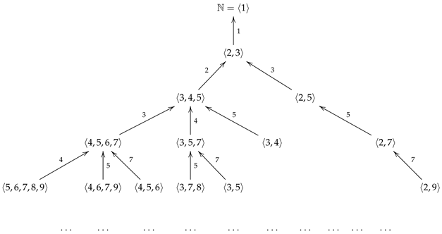
Observe that the number x, which appears on the edge $\begin{array}{c}P\hfill \\ \uparrow x\hfill \\ Q\hfill \end{array}$, indicates that $Q=P\setminus \left\{x\right\}$. In addition, observe that $\mathrm{F}\left(Q\right)=x$. The ellipsis indicates that the tree continues.

It is not possible to give an algorithm that computes all the elements of $\mathcal{R}$, because its cardinality is infinite. Therefore, our next objective in this section will be to design an algorithm that allows us to obtain all the elements of $\mathcal{R}$ with a specific genus.

Let $G=(V,E)$ be a rooted tree. We will call the depth of a vertex $v\in V$ in G the length of the only path that connects v with its root. It will be denoted by $\mathrm{d}\left(v\right)$. Let $n\in \mathbb{N}$; we denote by $\mathrm{N}(G,n)=\{x\in V\mid \mathrm{d}(x)=n\}$. The height of G, denoted by $\mathrm{h}\left(G\right)$, is the maximum of the set $\left\{\mathrm{d}\right(v)\mid v\in V\}$. Note that $\mathrm{h}\left(G\right)=max\{n\in \mathbb{N}\mid \mathrm{N}(G,n)\ne \varnothing \}$.

The following result is easily demonstrated:

Proposition 3.

Let $n\in \mathbb{N}$. The following statements are verified:

1. 

$\mathrm{N}\left(G\right(S),n+1)=\{S\in \mathcal{R}\mid S\mathit{is}a\mathit{child}\mathit{of}\mathit{an}\mathit{element}\mathit{of}\mathrm{N}(G\left(\mathcal{R}\right),n\left)\right\}$.

2. 

$\mathrm{N}\left(G\right(\mathcal{R}),n)=\{S\in \mathcal{R}\mid \mathrm{g}(S)=n\}$.

3. 

The tree $G\left(\mathcal{R}\right)$ has an infinite height.

As a consequence of Proposition 3, we have the next result.

Corollary 1.

With the above notation, we have $\mathbb{N}=\left\{\mathrm{g}\right(S)\mid S\in \mathcal{R}\}$.

Now, we are in conditions to present an algorithm that computes all the elements of $\mathcal{R}$ with a given genus.

Algorithm 1 Computation of $\{S\in \mathcal{R}\mid \mathrm{g}(S)=g\}$

Input: A non negative integer $g.$ Output: $\{S\in \mathcal{R}\mid \mathrm{g}(S)=g\}.$ (1) $A=\left\{\mathbb{N}\right\}$, $i=0.$ (2) If $i=g$, then return A and stop. (3) For all $S\in A$ compute $\alpha \left(S\right)=\{x\in \mathrm{msg}\left(S\right)\mid x>\mathrm{F}\left(S\right) \mathrm{and} s+\mathrm{r}\left(s\right)\ne x \mathrm{for} \mathrm{all} s\in S \mathrm{such} \mathrm{that} {\displaystyle \frac{x}{2}}\le s<x\}.$ (4) ${\displaystyle A:=\bigcup _{S\in A}\{S\setminus \left\{x\right\}\mid x\in \alpha \left(S\right)\}}$, $i:=i+1$ and go to Step $\left(2\right).$

In what follows, we illustrate the operation of this algorithm.

Example 1.

We will determine the set $\{S\in \mathcal{R}\mid \mathrm{g}(S)=2\}$, by applying Algorithm 1 as follows:

• $A=\left\{\mathbb{N}\right\}$, $i=0$.
• $\alpha \left(\mathbb{N}\right)=\left\{1\right\}$.
• $A=\{⟨2,3⟩\}$, $i=1$.
• $\alpha (⟨2,3⟩)=\{2,3\}$.
• $A=\{⟨3,4,5⟩,⟨2,5⟩\}$, $i=2$.
• $\{S\in \mathcal{R}\mid \mathrm{g}(S)=2\}=\{⟨3,4,5⟩,⟨2,5⟩\}$.

We will end this section by posing the following two questions whose answers could be helped by Algorithm 1:

• Do the elements of set $\mathcal{R}$ satisfy the conjecture of Bras-Amorós?. That is $\#\{S\in \mathcal{R}\mid \mathrm{g}(S)=g\}\le \#\{S\in \mathcal{R}\mid \mathrm{g}(S)=g+1\}$ for all $g\in \mathbb{N}$?
• Do the elements of set $\mathcal{R}$ satisfy Wilf’s conjecture? That is, if $S\in \mathcal{R}$, then $\mathrm{e}\left(S\right)\mathrm{g}\left(S\right)\le \left(\mathrm{e}\right(S)-1)\left(\mathrm{F}\right(S)+1)$?

3. $\mathcal{R}$-System of Generators

By Proposition 1, we know that the finite intersection of elements from $\mathcal{R}$ is again an element of $\mathcal{R}$. The intersection of infinite elements of $\mathcal{R}$ in general is not an element of $\mathcal{R}$, as we show in the following example:

Example 2.

For every $n\in \mathbb{N}$, let $S_n=\{0,n,\to \}$. It is clear that $S_n\in \mathcal{R}$ for all $n\in \mathbb{N}$ and ${\displaystyle \bigcap _{n\in \mathbb{N}}{S}_n=\left\{0\right\}\notin \mathcal{R}}$.

Since the intersection of any collection of elements from $\mathcal{R}$, whether finite or infinite, is invariably a submonoid of $(\mathbb{N},+)$, we are led to the following definition. An $\mathcal{R}$-monoid is a submonoid of $(\mathbb{N},+)$ that is obtainable as the intersection of elements from $\mathcal{R}$.

Given $X\subseteq \mathbb{N}$, then the intersection of all elements of $\mathcal{R}$ that contains X, will be denoted by $\mathcal{R}\left[X\right]$.

The following result has an immediate proof.

Proposition 4.

If $X\subseteq \mathbb{N}$, then $\mathcal{R}\left[X\right]$ is the smallest $\mathcal{R}$-monoid that contains X.

If $X\subseteq \mathbb{N}$ and $\mathcal{R}\left[X\right]=M$, then X is called a $\mathcal{R}$-system of generators of M. In addition, if $M\ne \mathcal{R}\left[Y\right]$ for every $Y⊊X$, we will say that X is a $\mathcal{R}$-minimal system of generators of M.

By applying Proposition 1 and ([37], Theorem 18), we obtain the following result:

Theorem 2.

Every $\mathcal{R}$-monoid has a unique $\mathcal{R}$-minimal system of generators.

Given M, an $\mathcal{R}$-monoid, denoted by $\mathcal{R}\mathrm{msg}\left(M\right)$, is the $\mathcal{R}$-minimal system of generators of M.

The next result is easily verified.

Proposition 5.

Let M be an $\mathcal{R}$-monoid. Then, $\mathcal{R}\mathrm{msg}\left(M\right)\subseteq \mathrm{msg}\left(M\right)$.

If M is an $\mathcal{R}$-monoid, then the cardinality of $\mathcal{R}\mathrm{msg}\left(M\right)$ will be called the $\mathcal{R}$-rank of M, and we denote it by $\mathcal{R}\mathrm{rank}\left(M\right)$.

From Theorem 2 and Proposition 5, the following result can be obtained:

Corollary 2.

The set of all $\mathcal{R}$-monoids is $\left\{\mathcal{R}\right[X]\mid X\mathit{is} a \mathit{finite} \mathit{subset} \mathit{of} \mathbb{N}\setminus \{0\left\}\right\}$.

Lemma 3.

Let M be an $\mathcal{R}$-monoid. Then, $M\in \mathcal{R}$ if and only if M is a numerical semigroup.

Proof. (Necessity).

If $M\in \mathcal{R}$, then by definition M is a numerical semigroup.

(Sufficiency). As M is an $\mathcal{R}$-monoid, then there is a family $\{S_i\mid i\in I\}$ of elements from $\mathcal{R}$ such that $M={\bigcap }_{i\in I}{S}_i$. If $x\in M\setminus \left\{0\right\}$, then $x\in S_i\setminus \left\{0\right\}$ for all $i\in I$ and so $x+\mathrm{r}\left(x\right)\in S_i$ for all $i\in I$. Therefore, $x+\mathrm{r}\left(x\right)\in M$, and consequently $M\in \mathcal{R}$.    □

For $a,b\in \mathbb{Z}$, we denote by $a\mid b$ if $b=ca$ for some $c\in \mathbb{Z}$. Or else, a is said not to divide b, which is represented by the notation $a\nmid b$.

Proposition 6.

Let $X\subseteq \mathbb{N}\setminus \left\{0\right\}$. Then, $\mathcal{R}\left[X\right]$ is an element of $\mathcal{R}$ if and only if $gcd\left(X\right)=1$.

Proof. (Necessity).

We suppose that $gcd\left(X\right)=d\ne 1$. Then there is a positive prime p such that $p\mid d$. Let $S(p,n)=⟨p⟩\cup \{n,\to \}$ for all $n\in \mathbb{N}$. It is clear that $S(p,n)$ is an element of $\mathcal{R}$ that contains X for all $n\in \mathbb{N}$. Therefore, $\mathcal{R}\left[X\right]\subseteq {\bigcap }_{n\in \mathbb{N}}S(p,n)=⟨p⟩$ and so $\mathcal{R}\left[X\right]$ is not a numerical semigroup. Hence $\mathcal{R}\left[X\right]$ is not an element of $\mathcal{R}$.

(Sufficiency). As $gcd\left(X\right)=1$ and $X\subseteq \mathcal{R}\left[X\right]$, then we deduce that $\mathcal{R}\left[X\right]$ is a numerical semigroup. By applying Proposition 4 and Lemma 3, we can conclude that $\mathcal{R}\left[X\right]$ is an element of $\mathcal{R}$.    □

The next result can be obtained by applying Corollary 2 and Proposition 6 and it gives us a complete description of the set of $\mathcal{R}$.

Corollary 3.

With the above notation, $\mathcal{R}=\left\{\mathcal{R}\right[X]\mid X\subseteq \mathbb{N}\setminus \{0\},X is finite and gcd(X)=1\}$.

We now aim to develop an algorithmic procedure for computing $\mathcal{R}\left[X\right]$ from a finite set $X\subset \mathbb{N}\setminus \left\{0\right\}$ such that $gcd\left(X\right)=1$. With this goal in mind, the following definition is required. An element x of a numerical semigroup S is called small if $x<\mathrm{F}\left(S\right)$. Denote by $\mathrm{N}\left(S\right)=\{s\in S\mid s<\mathrm{F}(S\left)\right\}$. Let $\mathrm{n}\left(S\right)$ denote the cardinality of $\mathrm{N}\left(S\right)$. It is obvious that $\mathrm{g}\left(S\right)+\mathrm{n}\left(S\right)=\mathrm{F}\left(S\right)+1$.

Now we have all the necessary ingredients to show the algorithm that allows us to obtain set $\mathcal{R}\left[X\right]$.

Algorithm 2 Computation of $\mathcal{R}\left[X\right]$

Input: A finite subset X of $\mathbb{N}\setminus \left\{0\right\}$ such that $gcd\left(X\right)=1.$ Output: $\mathcal{R}\left[X\right].$ (1) $S=⟨X⟩.$ (2) $B\left(S\right)=\{s+\mathrm{r}(s)\mid s\in \mathrm{N}(S)\setminus \{0\} \mathrm{and} s+\mathrm{r}(s)\notin S\}.$ (3) If $B\left(S\right)=\varnothing$ then return S and stop. (4) $S=⟨\mathrm{msg}\left(S\right)\cup B\left(S\right)⟩$ and go to Step $\left(2\right).$

Below we show, with an example, how the previous algorithm works.

Example 3.

By applying Algorithm 2, we proceed to calculate the set $\mathcal{R}\left[\right\{4,9\left\}\right]$ as follows:

• $S=⟨4,9⟩=\{0,4,8,9,12,13,16,17,18,20,21,22,24,\to \}$.
• $B\left(S\right)=\{6,10\}$.
• $S=⟨4,9,6,10⟩=⟨4,6,9⟩=\{0,4,6,8,9,10,12,\to \}$.
• $B\left(S\right)=\varnothing$.
• $\mathcal{R}\left[\right\{4,9\left\}\right]=⟨4,6,9⟩$.

Observe that $\{S\in \mathcal{R}\mid \mathcal{R}\mathrm{rank}(S)=1\}=\left\{\mathbb{N}\right\}$. The following result is easy to prove and tells us what the set $\{S\in \mathcal{R}\mid \mathcal{R}\mathrm{rank}(S)=2\}$ is like.

Proposition 7.

Let $a,b\in \mathbb{N}\setminus \{0,1\}$ with $gcd(a,b)=1$. Then $\mathcal{R}\left[\right\{a,b\left\}\right]$ is an element of $\mathcal{R}$ with $\mathcal{R}$-rank two. Moreover, every element of $\mathcal{R}$ with $\mathcal{R}$-rank two has this form.

We will conclude this section by posing the following problem: If $\{a,b\}\subseteq \mathbb{N}\setminus \{0,1\}$ and $gcd(a,b)=1$, to find formulas based on a and b that calculate the Frobenius number, the genus and the embedding dimension of $\mathcal{R}\left[\right\{a,b\left\}\right]$.

4. Radical Numerical Semigroups with a Given Frobenius Number

We say that a family $\mathcal{C}$ of numerical semigroups is a covariety if it verifies the following conditions:

• There is the minimum, with respect to inclusion order, of $\mathcal{C}$.
• If $\{S_1,S_2\}\subseteq \mathcal{C}$, then $S_1\cap S_2\in \mathcal{C}$.
• Let $S\in \mathcal{C}$ with $S\ne min\left(\mathcal{C}\right)$, then $S\setminus \left\{\mathrm{m}\right(S\left)\right\}\in \mathcal{C}$.

Denote by $\mathcal{R}\left(F\right)=\{S\in \mathcal{R}\mid \mathrm{F}(S)=F\}$, where F is a positive integer.

Proposition 8.

$\mathcal{R}\left(F\right)$ is a covariety for every positive integer F as follows:

Proof. 

• It is trivial that the minimum of $\mathcal{R}\left(F\right)$ is $\{0,F+1,\to \}$.
• If $\{S,T\}\subseteq \mathcal{R}\left(F\right)$, then by Lemma 1, we know that $S\cap T$ is a numerical semigroup and $\mathrm{F}(S\cap T)=F$. By Proposition 1, we have that $S\cap T\in \mathcal{R}$ and so $S\cap T\in \mathcal{R}\left(F\right)$.
• If $S\in \mathcal{R}\left(F\right)$ and $S\ne \{0,F+1,\to \}$, then $\mathrm{m}\left(S\right)<F$. By applying Lemma 2, we have that $S\setminus \left\{\mathrm{m}\right(S\left)\right\}$ is a numerical semigroup. As $\mathrm{m}\left(S\right)<F$, then $\mathrm{F}(S\setminus \{\mathrm{m}\left(S\right)\left\}\right)=F$. If $s\in S\setminus \{0,\mathrm{m}(S\left)\right\}$, then $s>\mathrm{m}\left(S\right)$ and thus $s+\mathrm{r}\left(s\right)\in S\setminus \left\{\mathrm{m}\right(S\left)\right\}$. Therefore, $S\setminus \left\{\mathrm{m}\right(S\left)\right\}\in \mathcal{R}\left(F\right)$.

   □

We define the graph $\mathrm{G}\left(\mathcal{R}\right(F\left)\right)$ in the following way: $\mathcal{R}\left(F\right)$ is its set of vertices, and $(S,T)\in \mathcal{R}\left(F\right)\times \mathcal{R}\left(F\right)$ is an edge if and only if $T=S\setminus \left\{\mathrm{m}\right(S\left)\right\}$.

The next result is a direct consequence from Proposition 8 and ([37], Proposition 2.3).

Theorem 3.

If $F\in \mathbb{N}\setminus \left\{0\right\}$, then $\mathrm{G}\left(\mathcal{R}\right(F\left)\right)$ is a tree and the set $\{0,F+1,\to \}$ is its root.

We now proceed to characterize the children of an arbitrary vertex in the tree $\mathrm{G}\left(\mathcal{R}\right(F\left)\right)$. To this end, we introduce the following definition. An integer x is a special gap of a numerical semigroup S if $x\notin S$ and $S\cup \left\{x\right\}$ is a numerical semigroup. The set formed by the special gaps of S will be denoted by $\mathrm{S}G\left(S\right)$.

The following result, derived from Proposition 8 and ([37], Proposition 2.4), identifies the children of any given vertex in $\mathrm{G}\left(\mathcal{R}\right(F\left)\right)$.

Proposition 9.

If $F\in \mathbb{N}\setminus \left\{0\right\}$ and $S\in \mathcal{R}\left(F\right)$, then the set formed by the children of S in the tree $\mathrm{G}\left(\mathcal{R}\right(F\left)\right)$ is $\{S\cup \{x\}\mid x\in \mathrm{S}G(S),x<\mathrm{m}(S) and S\cup \{x\}\in \mathcal{R}(F\left)\right\}$.

A straightforward verification shows the following result:

Proposition 10.

Let $F\in \mathbb{N}\setminus \left\{0\right\}$, $S\in \mathcal{R}\left(F\right)$ and $x\in \mathrm{S}G\left(S\right)$ such that $x\ne F$. Then $S\cup \left\{x\right\}\in \mathcal{R}\left(F\right)$ if and only if $x+\mathrm{r}\left(x\right)\in S$.

By applying the comment after the Proposition 2, Theorem 3 and Propositions 9 and 10, we can build the tree $\mathrm{G}\left(\mathcal{R}\right(7\left)\right)$ which is shown below.

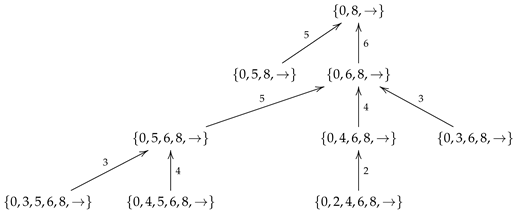
Note that the label x on the edge $\begin{array}{c}P\hfill \\ \uparrow x\hfill \\ Q\hfill \end{array}$ serves to indicate that $Q=P\cup \left\{x\right\}$. Moreover, observe that $\mathrm{m}\left(Q\right)=x$.

Let S be a numerical semigroup and $n\in S\setminus \left\{0\right\}$. The Apéry set of n in S (see [41]) is defined as $\mathrm{Ap}(S,n)=\{s\in S\mid s-n\notin S\}$.

By ([1], Lemma 2.4), we obtain the following:

Lemma 4.

Let S be a numerical semigroup and $n\in S\setminus \left\{0\right\}$. Then, $\mathrm{Ap}(S,n)=\{0=w(0),w(1),\dots ,w(n-1\left)\right\}$, where $w\left(i\right)$ is the least element of S congruent with i modulo n for all $i\in \{0,\dots ,n-1\}$.

Note 1.

Let S be a numerical semigroup, and we assume known $\mathrm{Ap}(S,n)$ for some $n\in S\setminus \left\{0\right\}$. Then we conclude the following:

1. 

We can readily determine $\mathrm{S}G\left(S\right)$, by applying ([37], Remark 1).

2. 

It is straightforward to compute $\mathrm{Ap}(S\cup \{x\},n)$ for all $x\in \mathrm{S}G\left(S\right)$ by using ([37], Remark 2).

All the required conditions are now in place to present the algorithm that computes the set $\mathcal{R}\left(F\right)$.

Algorithm 3 Computation of $\mathcal{R}\left(F\right)$

Input: A positive integer $F.$ Output: $\mathcal{R}\left(F\right).$ (1) $A=B=\left\{\right\{0,F+1,\to \left\}\right\}$ and $\mathrm{Ap}\left(\right\{0,F+1,\to \},F+1)=\{0,F+2,F+3,\cdots ,2F+1\}.$ (2) For every $S\in B$ computes $\theta \left(S\right)=\{x\in \mathrm{S}G(S)\mid x\ne F,x<\mathrm{m}(S) \mathrm{and} x+\mathrm{r}(x)\in S\}.$ (3) ${\displaystyle C=\bigcup _{S\in B}\{S\cup \left\{x\right\}\mid x\in \theta \left(S\right)\}.}$ (4) If $C=\varnothing$, then return A and stop. (5) $A:=A\cup C$ and $B:=C.$ (6) For all $S\in B$ computes $\mathrm{Ap}(S,F+1)$ and go to Step $\left(2\right).$

In the example below, we apply the above algorithm.

Example 4.

We are going to compute the set $\mathcal{R}\left(7\right)$, by applying Algorithm 3 as follows:

• $A=B=\left\{\right\{0,8,\to \left\}\right\}$ and $\mathrm{Ap}\left(\right\{0,8,\to \},8)=\{0,9,10,\cdots ,15\}$.
• $\theta \left(\right\{0,8,\to \left\}\right)=\{5,6\}$.
• $A=\left\{\right\{0,8,\to \},\{0,5,8,\to \},\{0,6,8,\to \left\}\right\}$ and $B=\left\{\right\{0,5,8,\to \},\{0,6,8,\to \left\}\right\}$.
• $\mathrm{Ap}\left(\right\{0,5,8,\to \},8)=\{0,5,9,10,11,12,14,15\}$ and
  $\mathrm{Ap}\left(\right\{0,6,8,\to \},8)=\{0,6,9,10,11,12,13,15\}$.
• $\theta \left(\right\{0,5,8,\to \left\}\right)=\varnothing$ and $\theta \left(\right\{0,6,8,\to \left\}\right)=\{3,4,5\}$.
• $A=\left\{\right\{0,8,\to \},\{0,5,8,\to \},\{0,6,8,\to \},\{0,3,6,8,\to \},\{0,4,6,8,\to \},\{0,5,6,8,\to \left\}\right\}$ and $B=\left\{\right\{0,3,6,8,\to \},\{0,4,6,8,\to \},\{0,5,6,8,\to \left\}\right\}$.
• $\mathrm{Ap}\left(\right\{0,3,6,8,\to \},8)=\{0,3,6,9,10,12,13,15\}$, $\mathrm{Ap}\left(\right\{0,4,6,8,\to \},8)=\{0,4,6,9,10,11,13,15\}$ and $\mathrm{Ap}\left(\right\{0,5,6,8,\to \},8)=\{0,5,6,9,10,11,12,15\}$.
• $\theta \left(\right\{0,3,6,8,\to \left\}\right)=\varnothing$, $\theta \left(\right\{0,4,6,8,\to \left\}\right)=\left\{2\right\}$ and $\theta \left(\right\{0,5,6,8,\to \left\}\right)=\{3,4\}$.
• $A=\left\{\right\{0,8,\to \},\{0,5,8,\to \},\{0,6,8,\to \},\{0,3,6,8,\to \},\{0,4,6,8,\to \},\{0,5,6,8,\to \},\{0,2,4,6,8,\to \},\{0,3,5,6,8,\to \},\{0,4,5,6,8,\to \left\}\right\}$ and $B=\left\{\right\{0,2,4,6,8,\to \},\{0,3,5,6,8,\to \},\{0,4,5,6,8,\to \left\}\right\}$.
• $\mathrm{Ap}\left(\right\{0,2,4,6,8,\to \},8)=\{0,2,4,6,9,11,13,15\}$, $\mathrm{Ap}\left(\right\{0,3,5,6,8,\to \},8)=\{0,3,5,6,9,10,12,15\}$ and $\mathrm{Ap}\left(\right\{0,4,5,6,8,\to \},8)=\{0,4,5,6,9,10,11,15\}$.
• $\theta \left(\right\{0,2,4,6,8,\to \left\}\right)=\varnothing$, $\theta \left(\right\{0,3,5,6,8,\to \left\}\right)=\varnothing$ and $\theta \left(\right\{0,4,5,6,8,\to \left\}\right)=\varnothing$.
• $\mathcal{R}\left(7\right)=\left\{\right\{0,8,\to \},\{0,5,8,\to \},\{0,6,8,\to \},\{0,3,6,8,\to \},\{0,4,6,8,\to \},\{0,5,6,8,\to \},\{0,2,4,6,8,\to \},\{0,3,5,6,8,\to \},\{0,4,5,6,8,\to \left\}\right\}$.

In ([1], Lemma 2.14), appears the following result:

Lemma 5.

Let S be a numerical semigroup. Then, ${\displaystyle \mathrm{g}\left(S\right)\ge \frac{\mathrm{F}\left(S\right)+1}{2}}$.

For a given rational number q, consider the set $\lceil q\rceil =min\{z\in \mathbb{Z}\mid q\le z\}$. From Lemma 5, we can deduce the below result.

Proposition 11.

If $F\in \mathbb{N}\setminus \left\{0\right\}$, then the height of the tree $\mathrm{G}\left(\mathcal{R}\right(F\left)\right)$ is less than or equal to ${\displaystyle F-⌈\frac{F+1}{2}⌉}$.

It is clear that if F is odd, then $⟨2,F+2⟩\in \mathcal{R}\left(F\right)$ and ${\displaystyle \mathrm{g}\left(⟨2,F+2⟩\right)=\frac{F+1}{2}}$. Therefore, if F is odd, we achieve the equality in Proposition 11. However, the bound that appears in Proposition 11, in general, is not achieved when F is even, since if we consider the tree $\mathrm{G}\left(\mathcal{R}\right(6\left)\right)$,

$$\begin{array}{c}\{0,7,\to \}\\ \uparrow 5\\ \{0,5,7,\to \}\end{array}$$

its height is 1 and ${\displaystyle 6-⌈\frac{6+1}{2}⌉=2}$.

5. Radical Numerical Semigroups with Fixed Multiplicity

A Frobenius pseudo-variety is a family $\mathcal{P}$ of numerical semigroups verifying the following conditions:

• $\mathcal{P}$ has a maximum with respect to inclusion order.
• If $\{S,T\}\subseteq \mathcal{P}$, then $S\cap T\in \mathcal{P}$.
• If $S\in \mathcal{P}$ and $S\ne max\left(\mathcal{P}\right)$, then $S\cup \left\{\mathrm{F}\right(S\left)\right\}\in \mathcal{P}$.

Our first aim in this section will be to prove that if $m\in \mathbb{N}\setminus \left\{0\right\}$, then ${\mathcal{R}}_m=\{S\in \mathcal{R}\mid \mathrm{m}\left(S\right)=m\}$ is a Frobenius pseudo-variety.

Proposition 12.

If $m\in \mathbb{N}\setminus \left\{0\right\}$, then ${\mathcal{R}}_m$ is a Frobenius pseudo-variety.

Proof. 

We are going to verify the conditions to be a Frobenius pseudo-variety as follows:

• It is trivial to see that $\{0,m,\to \}$ is the maximum of ${\mathcal{R}}_m$.
• If $\{S,T\}\subseteq {\mathcal{R}}_m$, then by Lemma 1, we know that $S\cap T$ is a numerical semigroup. By Proposition 1, we have $S\cap T\in \mathcal{R}$ and it is clear that $\mathrm{m}(S\cap T)=m$. Therefore, $S\cap T\in {\mathcal{R}}_m$.
• If $S\in {\mathcal{R}}_m$ and $S\ne \{0,m,\to \}$, then $\mathrm{F}\left(S\right)>m$. By using Lemma 1, we deduce that $S\cup \left\{\mathrm{F}\right(S\left)\right\}$ is a numerical semigroup with multiplicity m. By Proposition 1, we know that $S\cup \left\{\mathrm{F}\right(S\left)\right\}\in \mathcal{R}$ and so $S\cup \left\{\mathrm{F}\left(S\right)\right\}\in {\mathcal{R}}_m$.

   □

It is evident that ${\mathcal{R}}_1=\left\{\mathbb{N}\right\}$. In the next result we will see that if $m\in \mathbb{N}\setminus \{0,1\}$, then ${\mathcal{R}}_m$ is a set with infinite cardinality.

Proposition 13.

If $m\in \mathbb{N}\setminus \{0,1\}$, then ${\mathcal{R}}_m$ has infinite cardinality.

Proof. 

If $m\in \mathbb{N}\setminus \{0,1\}$, then there is a positive prime p such that $p\mid m$. For all $l\in \mathbb{N}\setminus \left\{0\right\}$, denote by $\mathrm{S}(p,l,m)=\left\{0\right\}\cup \{m+kp\mid k\in \mathbb{N}\}\cup \{lm,\to \}$. It is clear that $\mathrm{S}(p,l,m)\in {\mathcal{R}}_m$ and $\mathrm{F}\left(\mathrm{S}\right(p,l,m\left)\right)=lm-1$. Therefore, ${\mathcal{R}}_m$ is a set with infinite cardinality.    □

Define the graph $\mathrm{G}\left({\mathcal{R}}_m\right)$ in the following way: ${\mathcal{R}}_m$ is its set of vertices and $(S,T)\in {\mathcal{R}}_m\times {\mathcal{R}}_m$ is an edge if and only if $T=S\cup \left\{\mathrm{F}\right(S\left)\right\}$.

By applying Proposition 12 and ([38], Theorem 3), we obtain the following result:

Theorem 4.

If $m\in \mathbb{N}\setminus \{0,1\}$, then $\mathrm{G}\left({\mathcal{R}}_m\right)$ is a tree and $\{0,m,\to \}$ is its root. Moreover, the set formed by the children of a vertex S of this tree is $\{S\setminus \left\{x\right\}\mid x\in \mathrm{msg}\left(S\right),x>\mathrm{F}\left(S\right) and S\setminus \left\{x\right\}\in {\mathcal{R}}_m\}$.

By applying Lemma 2 and Proposition 2, it is easy to deduce the following result:

Proposition 14.

Let $S\in {\mathcal{R}}_m$ and $x\in \mathrm{msg}\left(S\right)$. Then, $S\setminus \left\{x\right\}\in {\mathcal{R}}_m$ if and only if $x\ne m$ and $s+\mathrm{r}\left(s\right)\ne x$ for all $s\in S$ such that ${\displaystyle \frac{x}{2}}\le s<x$.

By using the comment after Proposition 2, Theorem 4 and Proposition 14, we can recurrently build the tree $\mathrm{G}\left({\mathcal{R}}_4\right)$ shown below,

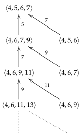
The number x appearing on the edge $\begin{array}{c}P\hfill \\ \uparrow x\hfill \\ Q\hfill \end{array}$ signifies that $Q=P\setminus \left\{x\right\}$. Furthermore, note that $\mathrm{F}\left(Q\right)=x$. The ellipsis signifies that the tree continues indefinitely.

By applying Proposition 13 and that $\{0,m,\to \}$ is the maximum of ${\mathcal{R}}_m$, we can easily deduce the next result.

Proposition 15.

If $m\in \mathbb{N}\setminus \{0,1\}$, then $\{\mathrm{g}\left(S\right)\mid S\in {\mathcal{R}}_m\}=\{m-1,\to \}$.

Applying all the previous results, we can now show an algorithm that allows us to obtain all the elements of ${\mathcal{R}}_m$ with a given genus.

Algorithm 4 Computation of $\{S\in {\mathcal{R}}_m\mid \mathrm{g}\left(S\right)=g\}$

Input: $m\in \mathbb{N}\setminus \{0,1\}$ and $g\in \{m-1,\to \}.$ Output: $\{S\in {\mathcal{R}}_m\mid \mathrm{g}\left(S\right)=g\}.$ (1) $A=\left\{\right\{0,m,\to \left\}\right\}$, $i=m-1.$ (2) If $i=g$, then return A and stop. (3) For every $S\in A$ computes $\gamma \left(S\right)=\{x\in \mathrm{msg}\left(S\right)\setminus \left\{m\right\}\mid x>\mathrm{F}\left(S\right) \mathrm{and} s+\mathrm{r}\left(s\right)\ne x \mathrm{for} \mathrm{all} s\in S,{\displaystyle \frac{x}{2}}\le s<x\}.$ (4) ${\displaystyle A=\bigcup _{S\in A}\{S\setminus \left\{x\right\}\mid x\in \gamma \left(S\right)\},}$$i=i+1$ and go to Step $\left(2\right).$

We finish the paper showing how the previous algorithm works.

Example 5.

We are going to compute the set $\{S\in {\mathcal{R}}_4\mid \mathrm{g}\left(S\right)=5\}$, by using Algorithm 4 as follows:

• $A=\{⟨4,5,6,7⟩\}$, $i=3$.
• $\gamma (⟨4,5,6,7⟩)=\{5,7\}$.
• $A=\{⟨4,6,7,9⟩,⟨4,5,6⟩\}$, $i=4$.
• $\gamma (⟨4,6,7,9⟩)=\{7,9\}$ and $\gamma (⟨4,5,6⟩)=\varnothing$.
• $A=\{⟨4,6,9,11⟩,⟨4,6,7⟩\}$, $i=5$.
• $\{S\in {\mathcal{R}}_4\mid \mathrm{g}\left(S\right)=5\}=\{⟨4,6,9,11⟩,⟨4,6,7⟩\}$.

6. Conclusions

In this work, and encouraged by some results from Number Theory and, in particular, the abc conjecture, we introduce the concept of a radical numerical semigroup.

We have proven that the set formed by all radical numerical semigroups is a Frobenius variety, and, as a consequence, we give an algorithm that computes all radical numerical semigroups with a given genus.

The paper also demonstrates that the set of radical numerical semigroups with Frobenius number F forms a covariety. Leveraging this fact, we develop an algorithm that computes all the radical numerical semigroups having F as their Frobenius number.

We have shown that the set formed by all the radical numerical semigroups of multiplicity m is a pseudo-Frobenius variety. This fact has allowed us to present an algorithm that computes all the radical numerical semigroups with fixed multiplicity and genus.

If $X\subseteq \mathbb{N}$ and $gcd\left(X\right)=1$, then in this work, we prove that there exists the smallest (with respect to inclusion order) radical numerical semigroup containing X. Furthermore, we have given an algorithm for obtaining such a numerical semigroup.

Finally, we have linked the study carried out with two important conjectures current in the theory of numerical semigroups: Wilf’s conjecture and Bras-Amorós conjecture. Specifically, we have left open the question of whether the family of radical numerical semigroups satisfies these conjectures.

References

- Rosales, J.C.; García-Sánchez, P.A. Numerical Semigroups; Springer: New York, NY, USA, 2009; Volume 20. [Google Scholar]
- Brauer, A. On a problem of partitions. Am. J. Math. 1942, 64, 299–312. [Google Scholar] [CrossRef] [Scilit]
- Brauer, A.; Schockley, J.E. On a problem of Frobenius. J. Reine Angew. Math. 1962, 211, 215–220. [Google Scholar]
- Curtis, F. On formulas for the Frobenius number of a numerical semigroup. Math. Scand. 1990, 67, 190–192. [Google Scholar] [CrossRef] [Scilit]
- Davison, J.L. On the linear Diophantine problem of Frobenius. J. Number Theory 1994, 48, 353–363. [Google Scholar] [CrossRef] [Scilit]
- Djawadi, M.; Hofmeister, G. Linear Diophantine problem. Arch. Math. 1996, 66, 19–29. [Google Scholar] [CrossRef] [Scilit]
- Johnson, S.M. A linear diophantine problem. Can. J. Math. 1960, 12, 390–398. [Google Scholar] [CrossRef] [Scilit]
- Selmer, E.S. On a linear diophantine problem. J. Reine Angew. Math. 1977, 293/294, 1–17. [Google Scholar]
- Sylvester, J.J. Mathematical questions with their solutions. Educ. Times 1884, 41, 21. [Google Scholar]
- Barucci, V.; Dobbs, D.E.; Fontana, M. Maximality Properties in Numerical Semigroups and Applications to One-Dimensional Analitycally Irreducible Local Domains. Mem. Am. Math. Soc. 1997, 598, 1–78. [Google Scholar]
- Bertin, J.; Carbonne, P. Semi-groupes d’entiers et application aux branches. J. Algebra. 1977, 49, 81–95. [Google Scholar] [CrossRef] [Scilit]
- Castellanos, J. A relation between the sequence of multiplicities and the semigroups of values of an algebroid curve. J. Pure Appl. Algebra 1986, 43, 119–127. [Google Scholar] [CrossRef] [Scilit]
- Delorme, C. Sous-monoïdes d’intersection complète de N. Ann. Sci. École Norm. Super. 1976, 9, 145–154. [Google Scholar] [CrossRef] [Scilit]
- Fröberg, R.; Gottlieb, G.; Häggkvist, R. On numerical semigroups. Semigroup Forum 1987, 35, 63–83. [Google Scholar] [CrossRef] [Scilit]
- Kunz, E. The value-semigroup of a one-dimensional Gorenstein ring. Proc. Am. Math. Soc. 1973, 25, 748–751. [Google Scholar] [CrossRef]
- Teissier, B. Appendice “Le Probléme des Modules Pour le Branches Planes”, Course Donné par O. Zariski au Centre de Math; Hermann, Éditeurs Dessciences et des Arts; de L’École Polytechnique: Paris, France, 1973. [Google Scholar]
- Watanabe, K. Some examples of one dimensional Gorenstein domains. Nagoya Math. J. 1973, 49, 101–109. [Google Scholar] [CrossRef] [Scilit]
- Ramírez Alfonsín, J.L. The Diophantine Frobenius Problem; Oxford University Press: London, UK, 2005. [Google Scholar]
- Sylvester, J.J. Problem 7382. In Educational Times and Journal of the College of Preceptors; New Ser; C.F. Hodgson & Son: Harrow, UK, 1883; Volume 36, p. 177. [Google Scholar]
- Wilf, H.S. A circle-of-lights algorithm for the “money-change problem”. Am. Math. Mon. 1978, 85, 562–565. [Google Scholar]
- Delgado, M. Conjeture of Wilf: A Survey Numerical Semigroups; Springer INdAM Series; Springer: Berlin/Heidelberg, Germany, 2018; Volume 40, pp. 39–62. [Google Scholar] [CrossRef] [Scilit]
- Delgado, M.; Eliahou, S.; Fromentin, A. A verification of Wilf’s conjeture up to genus 100. J. Algebra 2025, 664, 150–163. [Google Scholar] [CrossRef] [Scilit]
- Eliahou, S. Wilf’s conjeture and Macaulay’s Theorem. J. Eur. Math. Soc. 2018, 20, 2105–2129. [Google Scholar] [CrossRef] [Scilit]
- Eliahou, S. A graph-theoretic approach to Wilf’s conjeture. Electron. J. Comb. 2020, 27, 15–31. [Google Scholar]
- Eliahou, S.; Fromentin, J. Near-misses in Wilf’s conjeture. Semigroup Forum 2019, 98, 285–298. [Google Scholar] [CrossRef] [Scilit]
- Bras-Amorós, M. Bound on the number of numerical semigroups of a given genus. J. Pure Appl. Algebra 2008, 213, 997–1001. [Google Scholar] [CrossRef] [Scilit]
- Bras-Amorós, M. Fibonacci-like behavior of the number of numerical semigroups of a given genus. Semigroup Forum 2008, 76, 379–384. [Google Scholar] [CrossRef] [Scilit]
- Elizalde, S. Improved bounds on the number of numerical semigroup of a given genus. J. Pure Appl. Algebra 2010, 214, 1862–1873. [Google Scholar] [CrossRef] [Scilit]
- Kaplan, N. Counting numerical semigroups by genus and some cases of a question of Wilf. J. Pure Appl. Algebra 2012, 216, 1016–1032. [Google Scholar] [CrossRef] [Scilit]
- Blanco, V.; Rosales, J.C. The set of numerical semigroups of a given genus. Semigroup Forum 2012, 85, 255–267. [Google Scholar] [CrossRef] [Scilit]
- Zhai, A. Fibonacci-like growth of numerical semigroups with a given genus. Semigroup Forum 2013, 86, 634–662. [Google Scholar] [CrossRef] [Scilit]
- Baker, A. Experiments on the abc-conjecture. Publ. Math. Debr. 2012, 65, 253–260. [Google Scholar] [CrossRef] [Scilit]
- Nitaj, A. La conjecture abc. Enseign. Math. 1996, 42, 3–24. [Google Scholar]
- Oesterlé, J. Nouvelles approches du théorème de Fermat. Astérisque Séminaire Bourbaki exp 694 1988, 161, 165–186. [Google Scholar]
- Pasten, H.; Sepúlveda-Manzo, R. On the abc and the abcd conjectures. Bull. Braz. Math. Soc. 2025, 56, 54. [Google Scholar] [CrossRef] [Scilit]
- Rosales, J.C. Families of numerical semigroups closed under finite intersection and for the Frobenius number. Houst. J. Math. 2008, 34, 339–348. [Google Scholar]
- Moreno-Frías, M.A.; Rosales, J.C. The The covariety of numerical semigroups with fixed Frobenius number. J. Algebr. Comb. 2024, 60, 555–568. [Google Scholar] [CrossRef] [Scilit]
- Robles-Pérez, A.M.; Rosales, J.C. Frobenius pseudo-varieties in numerical semigroups. Ann. Mat. Pura Appl. 2015, 194, 275–287. [Google Scholar] [CrossRef] [Scilit]
- Delgado, M.; García-Sánchez, P.A.; Morais, J. NumericalSgps, A Package for Numerical Semigroups, Version 1.3.1; Refereed GAP Package. 2022. Available online: https://gap-packages.github.io/numericalsgps (accessed on 25 October 2025).
- The GAP Group. GAP–Groups, Algorithms, and Programming, Version 4.15.1. 2025. Available online: https://www.gap-system.org (accessed on 25 October 2025).
- Apéry, R. Sur les branches superlinéaires des courbes algébriques. C. R. Acad. Sci. Paris 1946, 222, 1198–2000. [Google Scholar]
Disclaimer/Publisher’s Note: The statements, opinions and data contained in all publications are solely those of the individual author(s) and contributor(s) and not of MDPI and/or the editor(s). MDPI and/or the editor(s) disclaim responsibility for any injury to people or property resulting from any ideas, methods, instructions or products referred to in the content. |
© 2026 by the authors. Licensee MDPI, Basel, Switzerland. This article is an open access article distributed under the terms and conditions of the Creative Commons Attribution (CC BY) license.