Inference for the Chris–Jerry Lifetime Distribution Under Improved Adaptive Progressive Type-II Censoring for Physics and Engineering Data Modelling

Mohammed, Heba S.; Abo-Kasem, Osama E.; Elshahhat, Ahmed

doi:10.3390/axioms14090702

Abstract

This paper presents a comprehensive reliability analysis framework for the Chris–Jerry (CJ) lifetime distribution under an improved adaptive progressive Type-II censoring plan. The CJ model, recently introduced to capture skewed lifetime behaviors, is studied under a modified censoring structure designed to provide greater flexibility in terminating life-testing experiments. We derive maximum likelihood estimators for the CJ parameters and key reliability measures, including the reliability and hazard rate functions, and construct approximate confidence intervals using the observed Fisher information matrix and the delta method. To address the intractability of the likelihood function, Bayesian estimators are obtained under independent gamma priors and a squared-error loss function. Because the posterior distributions are not available in closed form, we apply the Metropolis–Hastings algorithm to generate Bayesian estimates and two types of credible intervals. A comprehensive simulation study evaluates the performance of the proposed estimation techniques under various censoring scenarios. The framework is further validated through two real-world datasets: one involving rainfall measurements and another concerning mechanical failure times. In both cases, the CJ model combined with the proposed censoring strategy demonstrates superior fit and reliability inference compared to competing models. These findings highlight the value of the CJ distribution, together with advanced censoring methods, for modeling lifetime data in physics and engineering applications.

Keywords:

Chris–Jerry distribution; improved censoring; likelihood and Bayesian estimation; MCMC; asymptotic and credible intervals; delta method; reliability metrics

MSC:

62F10; 62F15; 62N01; 62N02; 62N05

1. Introduction

Recently, the development of flexible lifetime distributions has become increasingly important for accurately modeling real-world phenomena, particularly in reliability and survival analysis. Among these, the Chris–Jerry (CJ(

ϑ

)) distribution, introduced by Onyekwere and Obulezi [1], has emerged as a valuable contribution to the statistical literature. Its density can take unimodal or decreasing shapes, while its hazard function can exhibit a bathtub shape. This model is notable for its ability to capture positively skewed data, enhancing its applicability across a wide range of practical scenarios. It also provides closed-form expressions for its probability density and cumulative distribution functions, which facilitate both theoretical derivations and computational implementation. This flexibility makes the CJ distribution particularly suitable for modeling failure times in engineering systems and biomedical studies. Furthermore, its structure supports effective parameter estimation using both classical and Bayesian methods, even under complex censoring schemes, as demonstrated by Alotaibi et al. [2]. These properties underscore the CJ distribution’s potential as a robust and versatile tool in statistical inference and reliability analysis.

Let Y be a non-negative continuous random variable representing a lifetime. If Y∼

CJ (ϑ)

with

ϑ > 0

, then the probability density function (PDF) and cumulative distribution function (CDF) of Y are given by

f (y; ϑ) = \frac{ϑ^{2}}{ϑ + 2} (1 + ϑ y^{2}) e^{- ϑ y}, y > 0,

(1)

and

F (y; ϑ) = 1 - [1 + \frac{ϑ y (ϑ y + 2)}{ϑ + 2}] e^{- ϑ y},

(2)

respectively.

The corresponding reliability function (RF) and hazard rate function (HRF), denoted by

R (\cdot)

and

h (\cdot)

, at a mission time

x > 0

, are given, respectively, by

R (x; ϑ) = [1 + \frac{ϑ x (ϑ x + 2)}{ϑ + 2}] e^{- ϑ x},

(3)

and

h (x; ϑ) = \frac{ϑ^{2} (1 + ϑ x^{2})}{ϑ x (ϑ x + 2) + ϑ + 2} .

(4)

Progressive Type-II censoring (T2-PC) has been widely used in reliability and survival analysis because of its advantages over conventional Type-II censoring (T2-C). One key benefit is the flexibility to remove functioning experimental units during the study, which is particularly valuable in industrial reliability assessments and clinical trials. In a typical T2-PC setup, suppose m failures are observed among n identical test units, where

1 \leq m \leq n

. A predetermined censoring scheme

S = (S_{1}, S_{2}, \dots, S_{m})

is specified before the experiment. At the first failure time, denoted

Y_{1 : m : n}

, a randomly chosen

S_{1}

units are withdrawn from the remaining

n - 1

units. After the second failure,

Y_{2 : m : n}

, another

S_{2}

units are removed from the remaining

n - 2 - S_{1}

units, and this process continues. After the m-th failure, all remaining units corresponding to

S_{m}

are censored, thus completing the experiment; see Balakrishnan and Cramer [3].

Within the hybrid censoring framework, Kundu and Joarder [4] introduced the progressive Type-I hybrid censoring (T1-PHC) scheme. Under this design, n units are observed according to a fixed progressive censoring plan

S

, and the experiment terminates at

T^{*} = min (t, Y_{m : m : n})

, where t is a pre-specified time threshold. However, a key limitation of the T1-PHC scheme is the potential for a reduced observed sample size, which can compromise the efficiency of inferential procedures. To address this issue, Ng et al. [5] proposed the adaptive T2-PC (T2-APC) scheme, which improves estimation precision. In this design, the number of failures m is predetermined, and although a censoring scheme

S

is initially specified, its elements can be adaptively modified during the course of the experiment. The sampling structure follows that of the T2-PC, but the stopping criterion is adjusted to enhance practical applicability.

Nonetheless, if the test units exhibit very long survival times, the overall experiment duration under the T2-APC design may become impractically long. To overcome this limitation, Yan et al. [6] recently proposed the improved T2-APC (IT2-APC) scheme. This approach generalizes both the T1-PHC and T2-APC designs and introduces two time thresholds,

t_{1}

and

t_{2}

, where

0 < t_{1} < t_{2} < \infty

, thereby imposing an upper bound on the total test duration. The IT2-APC retains the progressive unit-removal mechanism of the T2-PC, with m planned failures from a total of n test units under a censoring scheme

S

. After the first failure time,

Y_{1 : m : n}

, a random selection of

S_{1}

units is withdrawn from the remaining

n - 1

units. Subsequent failures trigger the removal of

S_{i}

units based on the updated risk set. Let

d_{1}

denote the number of observed failures by time

t_{1}

, and similarly, let

d_{2}

represent the number of observed failures by time

t_{2}

. Depending on when the experiment terminates, the observed data will correspond to one of the next several censoring scenarios:

Case-1: As $Y_{m : m : n} < t_{1}$ , stop the test at $Y_{m : m : n}$ .
Case-2: As $t_{1} \leq Y_{m : m : n} < t_{2}$ , reset $S$ as $S_{d_{1} + 1} = \dots = S_{m - 1} = 0$ , stop the test at $Y_{m : m : n}$ .
Case-3: As $t_{1} < t_{2} \leq Y_{m : m : n}$ , reset $S$ as $S_{d_{1} + 1} = \dots = S_{d_{2} - 1} = 0$ , stop the test at $t_{2}$ .

Let

y = {(Y_{1}, S_{1}), \dots, (Y_{d_{1}}, S_{d_{1}}), (Y_{d_{1} + 1}, 0), \dots, (Y_{d_{2} - 1}, 0), (Y_{d_{2}}, S^{★})}

be the observed sample of size

d_{2}

obtained under an IT2-APC scheme from a continuous population with PDF

f (\cdot)

and CDF

F (\cdot)

. The joint likelihood function (LF) of

ϑ

for this sample can be written as

L (ϑ ∣ y) \propto \prod_{i = 1}^{B} (f (y_{i}; ϑ)) \prod_{i = 1}^{A} ({[1 - F (y_{i}; ϑ)]}^{S_{i}}) ({[1 - F (T^{★}; ϑ)]}^{S^{★}}),

(5)

where

y_{i} \equiv Y_{i : m : n}

and A is a term free of parameter(s). To distinguish, Table 1 explains the binary operators of the IT2-APC scheme represented in the LF (5).

Table 1. Options of

A, B, T^{★}, S^{★}

and

(y_{i}, S_{i})

.

It is important to note that several well-known censoring schemes can be obtained as special cases of the IT2-APC design, including the following:

The T1-PHC, proposed by Kundu and Joarder [4], when $t = t_{1} = t_{2}$ ;
The T2-APC, proposed by Ng et al. [5], when $t_{2} \to \infty$ ;
The T2-PC, described by Balakrishnan and Cramer [3], when $t_{1} \to \infty$ ;
The T2-C, described by Bain and Engelhardt [7], when $t_{1} \to 0$ , $S_{i} = 0$ for $i = 1, 2, \dots, m - 1$ , and $S_{m} = n - m$ .

Essentially, the threshold

t_{1}

serves as an early warning of the progress of the experiment, while the threshold

t_{2}

indicates the absolute maximum allowable duration of the study. If the threshold

t_{2}

is reached before a pre-specified number of failures m occurs, the experiment is terminated at

t_{2}

. This modification addresses the limitation of the T2-APC design proposed by Ng et al. [5], in which the total test duration was not guaranteed. By introducing the upper bound

t_{2}

, the IT2-APC strategy ensures that the total experiment time will not exceed this limit. In the literature, several works have dealt with this censoring plan, including the Weibull distribution (Nassar and Elshahhat [8]), Burr Type-III (Asadi et al. [9]), Nadarajah–Haghighi (El-Sherpieny et al. [10]), and the power half-normal (Alqasem and Elshahhat [11]).

The rapid advancement of technology and digital systems has increased the demand for censoring schemes that are both flexible and computationally efficient, particularly for analyzing modern reliability data characterized by bounded measures such as proportions or failure rates. Recent developments in lifetime data analysis highlight the importance of adaptable censoring strategies supported by computationally intensive Bayesian inference techniques. These insights reflect the growing need for robust methodologies that can effectively handle small sample data, high levels of oversight, and application-based reliability studies in engineering, biomedical sciences, and physical sciences. Although the CJ distribution is structurally simple, its key advantage is its ability to capture bathtub-shaped hazard behavior. Censored observations, particularly those arising from the IT2-APC design, are common due to cost and time constraints, underscoring the need for adaptive censoring strategies. Integrating the CJ model with this censoring mechanism enhances both the precision and reliability of lifetime data analysis. Under the IT2-APC framework, this study is conducted with the following key objectives:

To estimate the model parameter $ϑ$ , as well as the RF $R (x)$ and HRF $h (x)$ , for the CJ distribution using both maximum likelihood and Bayesian approaches.
To construct confidence intervals for the parameters of interest based on the asymptotic properties of the maximum likelihood estimators (MLEs) and log-transformed MLEs (log-MLEs).
To derive the Bayesian estimates, highest posterior density (HPD) intervals, and Bayesian credible intervals (BCIs) for $ϑ$ , $R (x)$ , and $h (x)$ via Markov chain Monte Carlo (MCMC) methods.
To implement the estimation procedures in the R programming environment (version 4.2.2) using the maxLik package (Henningsen and Toomet [12]) for likelihood optimization and the coda package (Plummer et al. [13]) for MCMC diagnostics.
To assess the accuracy and efficiency of the proposed estimators through comprehensive simulation studies and multiple performance metrics.
To demonstrate the practical applicability of the CJ distribution by analyzing two real-world datasets from physics and engineering sectors.

The remainder of this paper is organized as follows: Section 2 and Section 3 present the frequentist and Bayesian estimation methods, respectively. Simulation results are discussed in Section 4, and two real-data applications are analyzed in Section 5. Finally, Section 6 summarizes the main findings and provides concluding remarks.

2. Likelihood Inference

This section focuses on the estimation of the MLEs for the CJ parameters

ϑ

,

R (x)

, and

h (x)

. The

(1 - α) 100 %

ACIs for

ϑ

,

R (x)

, and

h (x)

are derived using the observed Fisher information (FI) matrix together with the delta method. Using (1), (2), and (5), we can rewrite (5) as follows:

\begin{matrix} L (ϑ | y) \propto \frac{ϑ^{2 B} e^{- ϑ ξ}}{{(ϑ + 2)}^{n}} \prod_{i = 1}^{B} (1 + ϑ y_{i}^{2}) \prod_{i = 1}^{A} {[ψ (y_{i}; ϑ)]}^{S_{i}} {[ψ (T^{★}; ϑ)]}^{S^{★}}, \end{matrix}

(6)

where

n = B + \sum_{i = 1}^{A} S_{i} + S^{★}

,

ξ = T^{★} S^{★} + \sum_{i = 1}^{B} y_{i} + \sum_{i = 1}^{A} y_{i} S_{i}

, and

ψ (y_{i}; ϑ) = 2 + ϑ + ϑ y_{i} (ϑ y_{i} + 2)

. The corresponding log-LF of (6) becomes

\begin{matrix} log L (ϑ | y) & \propto - n log (ϑ + 2) + 2 B log (ϑ) - ϑ ξ + \sum_{i = 1}^{B} log (1 + ϑ y_{i}^{2}) \\ + \sum_{i = 1}^{A} S_{i} log [ψ (y_{i}; ϑ)] + S^{★} log [ψ (T^{★}; ϑ)] . \end{matrix}

(7)

Subsequently, the MLE of

ϑ

, denoted by

\hat{ϑ}

, is obtained by maximizing (7) and solving the following nonlinear normal equation:

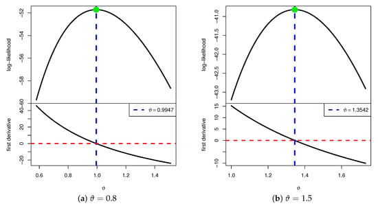
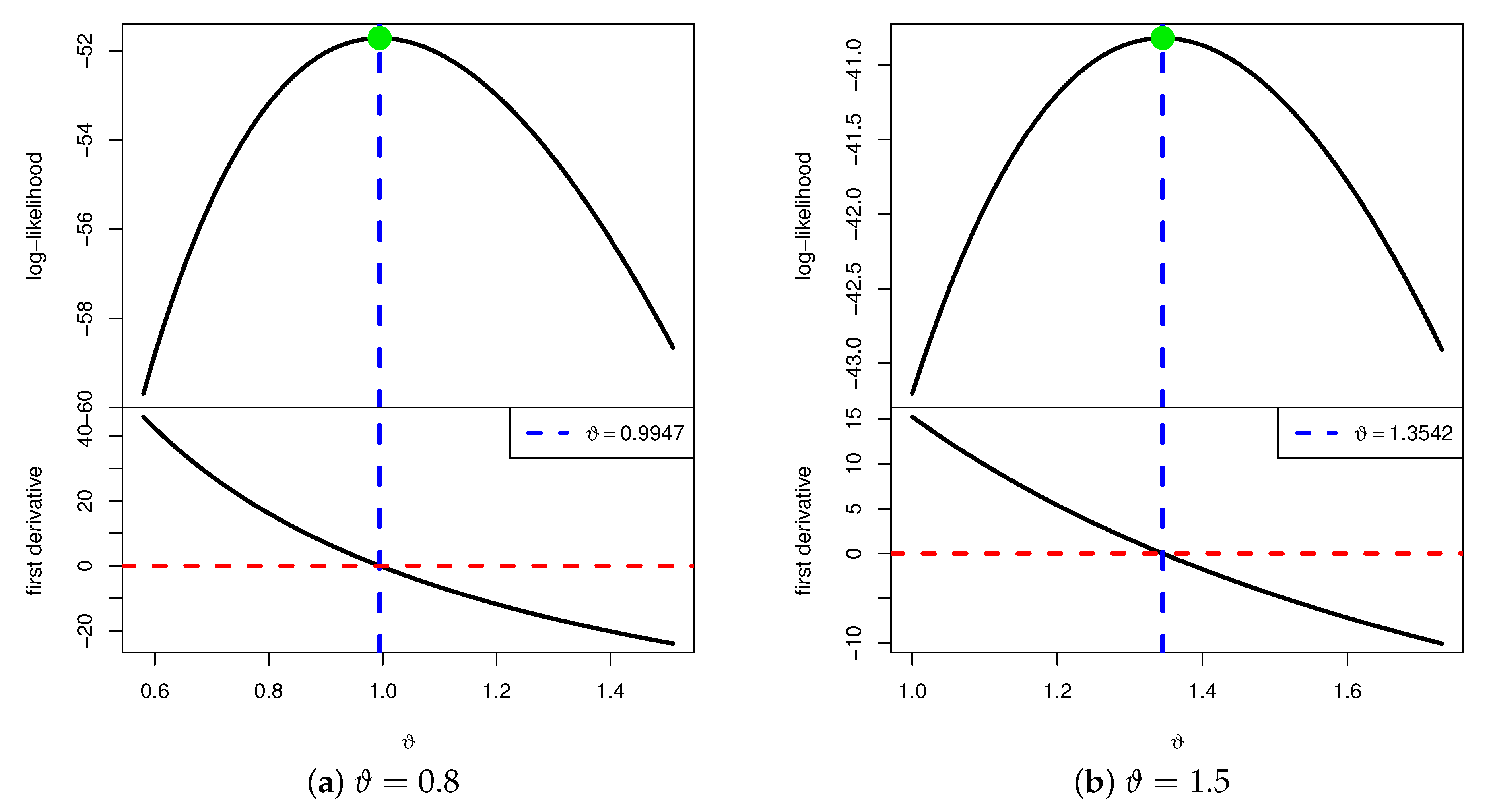
\begin{matrix} \frac{d log L (ϑ | y)}{d ϑ} & = 2 B ϑ^{- 1} - [ξ + n {(ϑ + 2)}^{- 1}] + \sum_{i = 1}^{B} [\frac{y_{i}^{2}}{1 + ϑ y_{i}^{2}}] \\ + \sum_{i = 1}^{A} S_{i} [\frac{1 + 2 y_{i} (ϑ y_{i} + 1)}{ψ (y_{i}; ϑ)}] {+ S^{★} [\frac{1 + 2 T^{★} (ϑ T^{★} + 1)}{ψ (T^{★}; ϑ)}]|}_{ϑ = \hat{ϑ}} = 0 . \end{matrix}

(8)

We now investigate the existence and uniqueness of

\hat{ϑ}

numerically by simulating an IT2-APC sample from the CJ distribution with parameters

ϑ = (0.8, 1.5)

, under the setup

n = 50

,

m = 25

,

(t_{1}, t_{2}) = (1, 2)

, and a uniformly T2-PC scheme. The numerical results yield MLEs of

ϑ

as 0.9947 and 1.3542 for

ϑ = (0.8, 1.5)

, respectively. Figure 1 displays the log-LF defined in (7) and the score function given in (8), plotted as functions of

ϑ

over a selected range. As shown, the vertical line representing the MLE of

ϑ

intersects the log-LF curve at its maximum and intersects the score function at zero. These observations confirm that, for each value of

ϑ

, the MLE exists and is unique.

Figure 1. The log-LF curve versus its score function curve.

The MLEs of RF and HRF, denoted

\hat{R} (x)

and

\hat{h} (x)

(for

x > 0

), are obtained by substituting

\hat{ϑ}

into Equations (2) and (4), yielding

\hat{R} (x) = [1 + \frac{\hat{ϑ} x (\hat{ϑ} x + 2)}{\hat{ϑ} + 2}] e^{- \hat{ϑ} x} and \hat{h} (x) = \frac{{\hat{ϑ}}^{2} (1 + \hat{ϑ} x^{2})}{\hat{ϑ} x (\hat{ϑ} x + 2) + \hat{ϑ} + 2} .

By applying the Newton–Raphson (NR) algorithm through the maxLik package in the R environment, the estimates

\hat{ϑ}

,

\hat{R} (x)

, and

\hat{h} (x)

can be efficiently computed.

In addition to the point estimates, constructing the

100 (1 - α) %

ACIs for the parameters

ϑ

,

R (x)

, and

h (x)

is of practical importance. Leveraging the asymptotic properties of the MLE

\hat{ϑ}

, these ACIs can be derived as follows. Specifically, the asymptotic distribution of

\hat{ϑ}

is approximately normal with mean

ϑ

and variance-covariance (VC) matrix

V (\cdot)

, which is typically obtained from the FI matrix

I (\cdot)

. Due to the analytical complexity of the FI, it is often more practical to approximate

V (\cdot)

using the observed FI matrix evaluated at

ϑ = \hat{ϑ}

, denoted by

{I (\cdot) |}_{ϑ = \hat{ϑ}}

. Consequently, the VC matrix is estimated as:

\begin{matrix} V (\hat{ϑ}) & = I^{- 1} {(ϑ) |}_{ϑ = \hat{ϑ}}, \\ = {[- \frac{d^{2} log L (ϑ | y)}{d ϑ^{2}}]}_{ϑ = \hat{ϑ}}^{- 1}, \end{matrix}

(9)

where

\begin{matrix} \frac{d^{2} log L (ϑ | y)}{d ϑ^{2}} & = - 2 B ϑ^{- 2} + n {(ϑ + 2)}^{- 2} - \sum_{i = 1}^{B} \frac{y_{i}^{4}}{{(1 + ϑ y_{i}^{2})}^{2}} \\ + \sum_{i = 1}^{A} S_{i} \{\frac{2 y_{i}^{2} [ψ (y_{i}; ϑ)] - {[2 y_{i} (ϑ y_{i} + 1) + 1]}^{2}}{{[ψ (y_{i}; ϑ)]}^{2}}\} \\ + S^{★} \{\frac{2 {T^{★}}^{2} [ψ (T^{★}; ϑ)] - {[2 T^{★} (ϑ T^{★} + 1) + 1]}^{2}}{{[ψ (T^{★}; ϑ)]}^{2}}\} . \end{matrix}

On the other hand, to construct the

100 (1 - α) %

ACIs for the RF

R (x)

and HRF

h (x)

, it is first necessary to estimate the variances of their respective estimators,

\hat{R} (x)

and

\hat{h} (x)

. A widely used approach for this purpose is the delta method, which approximates these variances—denoted by

{\hat{V}}_{\hat{R}}

and

{\hat{V}}_{\hat{h}}

, respectively. Following the treatment in Greene [14], the delta method assumes that

\hat{R} (x)

is approximately normally distributed with mean

R (x)

and variance

{\hat{V}}_{\hat{R}}

, and similarly,

\hat{h} (x)

is approximately normal with mean

h (x)

and variance

{\hat{V}}_{\hat{h}}

.

Accordingly, the quantities of

{\hat{V}}_{\hat{R}}

and

{\hat{V}}_{\hat{h}}

are given, respectively, by:

{\hat{V}}_{\hat{R}} = {C_{R} V (ϑ) C_{R}^{⊤}|}_{ϑ = \hat{ϑ}} and {\hat{V}}_{\hat{h}} = {C_{h} V (ϑ) C_{h}^{⊤}|}_{ϑ = \hat{ϑ}},

where

C_{R} = x e^{- ϑ x} [{(ϑ + 2)}^{- 1} (2 + ϑ {2 x - ({(ϑ + 2)}^{- 1} + x) (2 + ϑ x)}) - 1]

C_{h} = \frac{ϑ (3 ϑ x^{2} + 2) ψ (x; ϑ) - ϑ^{2} (1 + ϑ x^{2}) ψ^{'} (x; ϑ)}{{[ψ (x; ϑ)]}^{2}} .

ψ (x; ϑ) = ϑ x (ϑ x + 2) + ϑ + 2 and ψ^{'} (x; ϑ) = 2 t (ϑ x + 1) + 1 .

Consequently, based on the normal approximation (NA) of

\hat{ϑ}

, the

(1 - α) 100 %

ACI using the NA-based approach (ACI-NA) at significance level

α

is given by

\hat{ϑ} \mp z_{\frac{α}{2}} \sqrt{V (\hat{ϑ})},

where

z_{\frac{α}{2}}

is the upper

{(\frac{α}{2})}^{t h}

standard Gaussian percentile point. Similarly, the ACI-NA estimator of

\hat{R} (x)

or

\hat{h} (x)

can be obtained.

A key limitation of the traditional ACI-NA approach is that it may produce negative lower bounds for parameters that are inherently restricted to positive values. In such cases, it is common to truncate negative bounds at zero, although this adjustment is heuristic rather than statistically rigorous. To address this limitation and improve the reliability of interval estimation, following Meeker and Escobar [15], the

(1 - α) 100 %

ACI based on the log-transform normal approximation (ACI-NL) is developed. Thus, the

(1 - α) 100 %

ACI-NL for

ϑ

is given by

log (\hat{ϑ}) \mp z_{\frac{α}{2}} \sqrt{V (log (\hat{ϑ}))},

which is equivalent to

\hat{ϑ} exp (\mp \frac{z_{\frac{α}{2}}}{\hat{ϑ}} \sqrt{V (\hat{ϑ})}) .

Similarly, the

(1 - α) 100 %

ACI-NL for

\hat{R} (x)

or

\hat{h} (x)

can be derived in the same manner.

3. Bayesian Inference

This section focuses on developing both point estimates and credible Bayesian intervals for

ϑ

,

R (x)

, and

h (x)

. Within the Bayesian paradigm, prior distributions and loss functions play a crucial role. Selecting an appropriate prior for an unknown parameter can be challenging. As emphasized by Gelman et al. [16], there is no universally accepted criterion for choosing a suitable prior in Bayesian analysis. Since the CJ parameter

ϑ

lies in the interval

(0, \infty)

, the gamma distribution provides a natural and tractable choice as a prior for

ϑ

. Assume

ϑ

∼

Gamma (a, b), a, b > 0,

where a and b are the hyperparameters. Then, the corresponding prior PDF, denoted by

Θ (ϑ)

, is given by

Θ (ϑ) = \frac{b^{a}}{Γ (a)} ϑ^{a - 1} e^{- b ϑ}, ϑ > 0 .

(10)

From (6) and (10), the posterior PDF (say

Υ (\cdot)

) of

ϑ

can be expresses as follows:

\begin{matrix} Υ (ϑ | y) \propto \frac{ϑ^{2 B + a - 1} e^{- ϑ (b + ξ)}}{{(ϑ + 2)}^{n}} \prod_{i = 1}^{B} (1 + ϑ y_{i}^{2}) \prod_{i = 1}^{A} {[ψ (y_{i}; ϑ)]}^{S_{i}} {[2 + ϑ + ϑ T^{★} (ϑ T^{★} + 2)]}^{S^{★}}, \end{matrix}

(11)

where its normalized term (say,

Ξ

) is given by

\begin{matrix} Ξ = \int_{0}^{\infty} Θ (ϑ) \times L (ϑ | y) d ϑ . \end{matrix}

It is worth noting that we adopt the squared-error loss (SEL) function, primarily because it is the most widely used symmetric loss function in Bayesian analysis. Nevertheless, the proposed methodology can be readily extended to obtain Bayesian estimates under alternative loss functions. Based on the posterior distribution in (11), and given the nonlinear structure of the likelihood function in (6), the Bayesian estimates of

ϑ

,

R (x)

, and

h (x)

under the SEL function are analytically intractable.

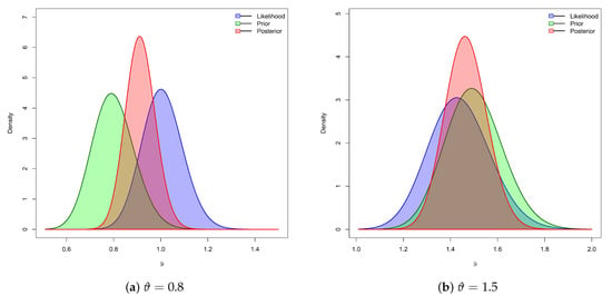
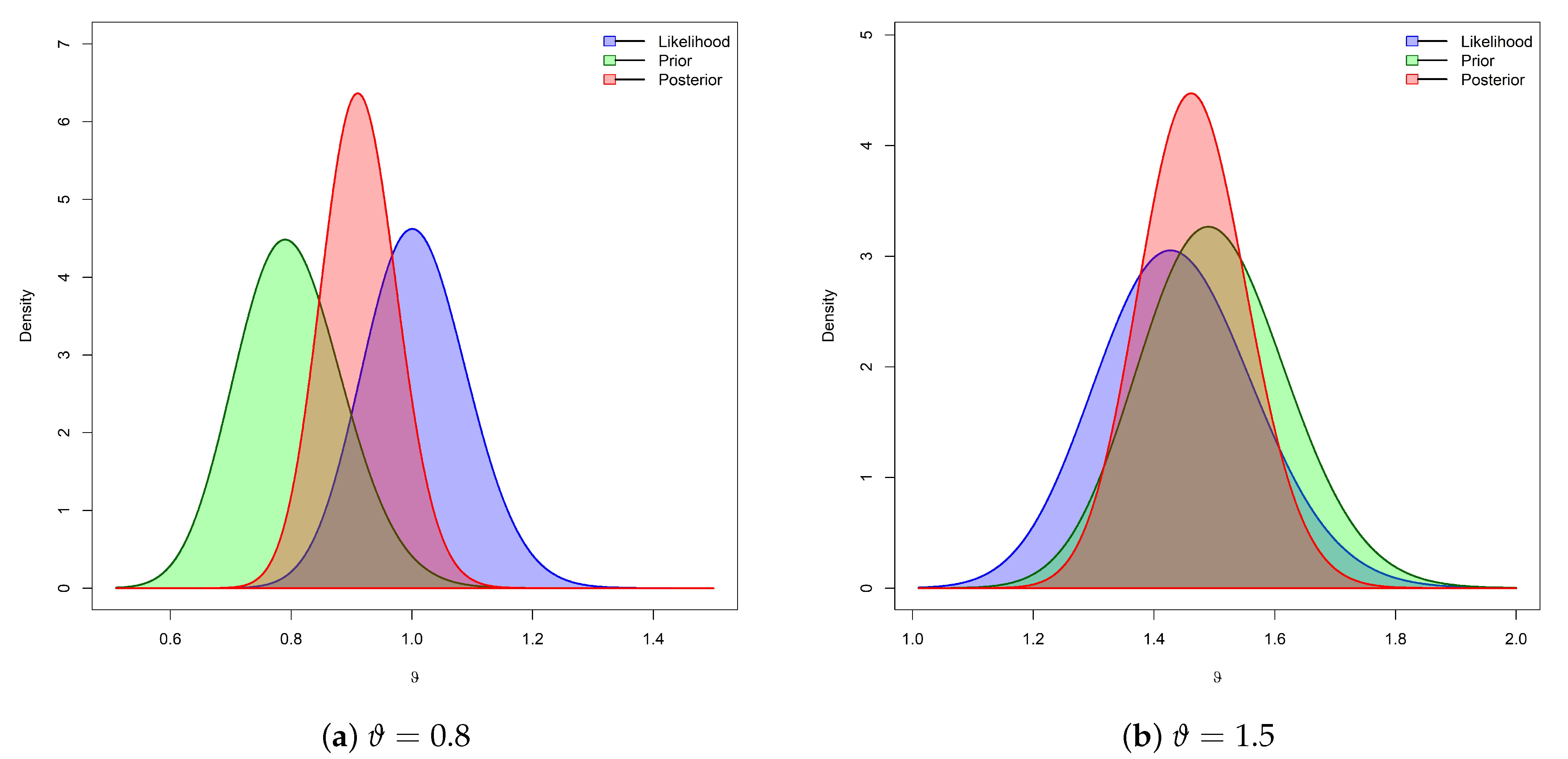
Consequently, by employing the MCMC technique, we generate Markovian samples from the posterior distribution in (11). Examining (11), it is evident that the PDF of

ϑ

cannot be expressed using any standard continuous statistical model. However, Figure 2 shows that the conditional PDF in (11) is approximately normal. Accordingly, following Algorithm 1, the Metropolis–Hastings (M-H) algorithm is employed to update the posterior samples of

ϑ

, after which the Bayesian estimates and the corresponding BCI/HPD interval estimates for

ϑ

,

R (x)

, and

h (x)

are computed.

Algorithm 1 The M-H Algorithm for

ϑ

,

R (x)

, and

h (x)

1:: Input: Initial estimate $\hat{ϑ}$ , estimated variance $\hat{V} (\hat{ϑ})$ , total iterations $N$ , burn-in $N^{\circ}$ , confidence level $(1 - α)$
2:: Output: Posterior mean $\tilde{ϑ}$ , BCI and HPD intervals of $ϑ$
3:: Set $ϑ^{(0)} \leftarrow \hat{ϑ}$
4:: Set $j \leftarrow 1$
5:: while $j \leq N$ do
6:: Generate $ϑ^{★} \sim N (ϑ^{(j - 1)}, \hat{V} (\hat{ϑ}))$
7:: Compute acceptance ratio:

$M \leftarrow min (1, \frac{Υ (ϑ^{★} ∣ y)}{Υ (ϑ^{(j - 1)} ∣ y)})$
8:: Generate $u \sim U (0, 1)$
9:: if $u \leq M$ then
10:: Set $ϑ^{(j)} \leftarrow ϑ^{★}$
11:: else
12:: Set $ϑ^{(j)} \leftarrow ϑ^{(j - 1)}$
13:: end if
14:: Update $R (x)$ and $h (x)$ using $ϑ^{(j)}$ in (3) and (4)
15:: Increment $j \leftarrow j + 1$
16:: end while
17:: Discard the first $N^{\circ}$ samples as burn-in
18:: Define $N^{•} = N - N^{\circ}$
19:: Compute:

$\tilde{ϑ} = \frac{1}{N^{•}} \sum_{j = N^{\circ} + 1}^{N} ϑ^{(j)}$
20:: Sort $ϑ^{(j)}$ for $j = N^{\circ} + 1, \dots, N$ in ascending order
21:: Compute the $(1 - α) 100 %$ BCI of $ϑ$ as:

$(ϑ_{(\frac{α}{2} N^{•})}, ϑ_{((1 - \frac{α}{2}) N^{•})})$
22:: Compute the $(1 - α) 100 %$ HPD interval of $ϑ$ as:

$(ϑ_{(j^{⊚})}, ϑ_{(j^{⊚} + (1 - α) N^{•})})$

where $j^{⊚}$ is the index that minimizes:

$ϑ_{(j + (1 - α) N^{•})} - ϑ_{(j)} for j = 1, \dots, α N^{•}$
23:: Redo Steps 19–22 for $R (x)$ and $h (x)$

Figure 2. The likelihood, prior, and posterior density shapes.

4. Monte Carlo Comparisons

To evaluate the precision and practical applicability of the estimated values of

ϑ

,

R (x)

, and

h (x)

discussed in the preceding sections, a series of Monte Carlo simulations is conducted. Specifically, following Algorithm 2, the IT2-APC procedure is replicated 1000 times for each selected value of

ϑ

(namely,

ϑ = 0.8

and

ϑ = 1.5

) to compute both point and interval estimates of the target parameters. For a fixed value of

x = 0.1

, the corresponding estimates of the reliability and hazard functions,

(R (x), h (x))

, are obtained as (0.97797, 0.21747) for

ϑ = 0.8

, and (0.94002, 0.59745) for

ϑ = 1.5

. The simulation experiments are carried out under various configurations involving threshold parameters

t_{i} (i = 1, 2)

, total sample sizes n, effective sample sizes m, and the progressive censoring scheme

S

. In particular, we consider

t_{1} \in {1, 2}

,

t_{2} \in {2, 4}

, and

n \in {30, 50, 80}

. Table 2 presents, for each value of n, several choices of failure sizes m along with their corresponding T2-PC schemes

S

. For illustrative purposes, a notation such as

5^{2}

indicates that five units are withdrawn from the experiment at each of the first two censoring stages.

Algorithm 2 Simulate IT2-APC data.

1:: Input: Assign values for n, m, $t_{i}, i = 1, 2$ , and $S$
2:: Set the true value of CJ( $ϑ$ ) parameter.
3:: Generate m independent uniform random variables $ε_{1}, ε_{2}, \dots, ε_{m} \sim U (0, 1)$
4:: for $i = 1$ to m do
5:: Compute $ϵ_{i} = ε_{i}^{{(i + \sum_{j = m - i + 1}^{m} S_{j})}^{- 1}}$
6:: end for
7:: for $i = 1$ to m do
8:: Compute $U_{i} = 1 - \prod_{j = m - i + 1}^{m} ϵ_{j}$
9:: end for
10:: for $i = 1$ to m do
11:: Compute $y_{i} = F^{- 1} (U_{i}; ϑ)$
12:: end for
13:: Observe $d_{1}$ failures at time $t_{1}$
14:: Discard observations $y_{i}$ for $i = d_{1} + 2, \dots, m$
15:: Set truncated sample size: $n_{trunc} = n - d_{1} - 1 - \sum_{i = 1}^{d_{1}} S_{i}$
16:: Simulate $m - d_{1} - 1$ order statistics $y_{d_{1} + 2}, \dots, y_{m}$ from truncated distribution:
PDF: $\frac{f (y)}{R (y_{d_{1} + 1})}$ where $R (\cdot)$ is the survival function
17:: if $y_{m} < t_{1} < t_{2}$ then
18:: Case 1: Stop test at $y_{m}$
19:: else if t₁ < y_m < t₂ then
20:: Case 2: Stop test at $y_{m}$
21:: else if t₁ < t₂ < y_m then
22:: Case 3: Stop test at $t_{2}$
23:: end if

Table 2. Different T2-PC designs in Monte Carlo simulations.

To further assess the sensitivity of the estimation procedures under the Bayesian framework, we consider two sets of hyperparameters for the CJ distribution under the two parameter settings. Following the prior elicitation strategy proposed by Kundu [17], we specify the hyperparameter values a and b in the gamma prior PDF, as follows:

At $ϑ = 0.8$ : Prior-1:(4,5) and Prior-2:(8,10);
At $ϑ = 1.5$ : Prior-1:(7.5,5) and Prior-2:(15,10).

Once 1000 IT2-APC datasets are generated, the frequentist estimates and their corresponding 95% ACI-NA and ACI-NL intervals for

ϑ

,

R (x)

, and

h (x)

are computed using the maxLik package. For the Bayesian analysis, 12,000 MCMC samples are drawn, with the first 2000 iterations discarded as burn-in. The resulting Bayesian estimates, along with their 95% BCI and HPD intervals for

ϑ

,

R (x)

, and

h (x)

, are then computed using the coda package.

Now, to evaluate the offered estimators obtained for the CJ(

ϑ

) parameter, we calculate the following metrics:

Mean Point Estimate: $MPE (\hat{ϑ}) = \frac{1}{1000} \sum_{i = 1}^{1000} {\hat{ϑ}}^{[i]},$
Root Mean Squared Error: $RMSE (\hat{ϑ}) = \sqrt{\frac{1}{1000} \sum_{i = 1}^{1000} {({\hat{ϑ}}^{[i]} - ϑ)}^{2}},$
Mean Relative Absolute Bias: $MRAB (\hat{ϑ}) = \frac{1}{1000} \sum_{i = 1}^{1000} {\hat{ϑ}}^{- 1} |{\hat{ϑ}}^{[i]} - ϑ|,$
Average Interval Length: ${AIL}_{95 %} (ϑ) = \frac{1}{1000} \sum_{i = 1}^{1000} (U_{{\hat{ϑ}}^{[i]}} - L_{{\hat{ϑ}}^{[i]}}),$
Coverage Percentage: ${CP}_{95 %} (ϑ) = \frac{1}{1000} \sum_{i = 1}^{1000} O_{(L_{{\hat{ϑ}}^{[i]}}; U_{{\hat{ϑ}}^{[i]}})} (ϑ),$
where ${\hat{ϑ}}^{[i]}$ is the desired estimate of $ϑ$ at ith sample, $O (\cdot)$ is indicator function, $(L (\cdot), U (\cdot))$ is two-sided of $(1 - α)$ asymptotic (or credible) of $ϑ$ . Similarly, the same precision metrics can be readily applied to $R (x)$ or $h (x)$ .

In Table 3, Table 4 and Table 5, the point estimation results—including MPEs (1st Col.), RMSEs (2nd Col.), and MRABs (3rd Col.)—for

ϑ

,

R (x)

and

h (x)

are reported. Meanwhile, Table 6, Table 7 and Table 8 present the AILs (1st Col.) and CPs (2nd Col.) for the same parameters. Based on these tables, we derive the following observations, focusing on the lowest RMSEs, MRABs, and AILs, and the highest CPs:

All results for $ϑ$ , $R (x)$ , and $h (x)$ exhibit consistently satisfactory performance across the simulated configurations. This demonstrates that both point and interval estimators remain stable under varying censoring levels, sample sizes, and prior specifications, highlighting the robustness of the proposed inference framework.
As n or m increase, the estimation accuracy of all model parameters improves. Larger sample sizes provide more information about the underlying failure-time distribution, reducing Monte Carlo variability and enhancing the coverage of interval estimates. A similar improvement is observed when the total number of removals, $\sum_{i = 1}^{m} S_{i}$ , decreases, as fewer removals preserve more observed failure times, thereby increasing the precision of parameter estimation.
Increasing the threshold values $t_{i}$ (for $i = 1, 2$ ) results in more precise parameter estimates. Specifically, the RMSEs, MRABs, and AILs for $ϑ$ , $R (x)$ , and $h (x)$ decrease, while the corresponding CPs increase. This indicates that longer censoring times provide more information about the tail behavior of the distribution, thereby improving inference for both the reliability and hazard functions.
As the value of $ϑ$ increases,
–
The RMSEs of $ϑ$ , $R (x)$ , and $h (x)$ increase, indicating that higher shape parameter values introduce heavier tails, which make estimation more challenging;
–
The MRABs of $ϑ$ and $h (x)$ decrease, whereas that of $R (x)$ increases, suggesting that bias behavior differs among the parameters, with $R (x)$ being more sensitive to changes in $ϑ$ than $h (x)$ ;
–
The AILs for all parameters increase, and the CPs tend to decrease, confirming that as $ϑ$ grows, the variability in estimates increases, making it harder to achieve nominal coverage levels.
For the parameter values considered ( $ϑ = 0.8, 1.5$ ), we observed that the RMSEs, MRABs, and AILs tend to increase as $ϑ$ becomes larger, while the CPs decrease. These patterns are empirical for the chosen parameter values and may not necessarily generalize to all possible values of $ϑ$ .
Bayesian estimates obtained via MCMC sampling, along with their corresponding credible intervals, exhibit superior robustness compared to their frequentist counterparts. The use of informative priors stabilizes inference, particularly under heavy censoring and small-sample scenarios, resulting in reduced RMSEs and narrower intervals without compromising coverage.
For each considered value of $ϑ$ , the Bayesian estimator based on Prior-2 consistently produces more accurate results than other approaches. This improvement is attributable to the lower prior variance of Prior-2 relative to Prior-1, which enables the posterior distribution to concentrate more efficiently around the true parameter values. A similar trend is observed when comparing asymptotic intervals (ACI-NA and ACI-NL) with Bayesian intervals (BCI and HPD), as the latter adapt more effectively to model complexity.
A comparative evaluation of the T2-PC designs listed in Table 2 reveals the following:
–
The point and interval estimates of $ϑ$ and $h (x)$ under configurations C $i [j]$ (for $i = 1, 2, 3$ and $j = 3, 6$ ) outperform those obtained from alternative schemes, indicating that these designs optimally balance the trade-off between sample size, number of removals, and censoring thresholds;
–
The estimates of $R (x)$ achieve the highest accuracy under configurations A $i [j]$ (for $i = 1, 2, 3$ and $j = 1, 4$ ), suggesting that reliability estimation may require different censoring strategies than those optimal for hazard estimation.
Comparing the proposed interval estimation techniques, we noted the following:
–
The ACI-NA approach outperforms ACI-NL for estimating $ϑ$ and $h (x)$ , whereas the reverse holds for $R (x)$ , indicating that linearization-based approximations are more effective for certain types of parameters;
–
The HPD method yields superior interval estimates for all parameters compared to the BCI approach, highlighting the efficiency of HPD intervals in summarizing posterior distributions;
–
Overall, Bayesian interval estimates (BCIs or HPD) consistently outperform asymptotic intervals (ACI-NA or ACI-NL), emphasizing the advantages of Bayesian inference in heavily censored experimental designs.
In conclusion, for practitioners involved in reliability analysis, the CJ lifetime population is best explored through a Bayesian framework using the MCMC methodology, particularly via the M-H sampling algorithm.

Table 3. Point estimations of

ϑ

.

Table 3. Point estimations of

ϑ

.

$(t_{1}, t_{2})$	$(n, m)$	T2-PC	MLE			MCMC
Prior→						1			2
For $ϑ = 0.8$
(1,2)	(30,10)	A1[1]	0.5502	0.3456	0.4151	0.8124	0.0878	0.0973	0.7688	0.0827	0.0808
		B1[2]	0.5161	0.3551	0.4319	0.8233	0.0916	0.1019	0.7777	0.0906	0.0874
		C1[3]	0.5502	0.2870	0.3291	0.8124	0.0860	0.0951	0.7688	0.0796	0.0808
	(30,20)	A1[4]	0.7572	0.1952	0.2176	0.8115	0.0841	0.0834	0.8568	0.0714	0.0792
		B1[5]	0.7287	0.1855	0.2077	0.8066	0.0825	0.0814	0.8523	0.0698	0.0779
		C1[6]	0.7321	0.1647	0.1879	0.8092	0.0771	0.0772	0.8561	0.0643	0.0727
	(50,20)	A2[1]	0.7114	0.1396	0.1521	0.8085	0.0700	0.0701	0.8524	0.0628	0.0664
		B2[2]	0.7184	0.1472	0.1592	0.8027	0.0728	0.0737	0.8453	0.0638	0.0675
		C2[3]	0.6948	0.1370	0.1493	0.8028	0.0673	0.0700	0.8453	0.0596	0.0651
	(50,40)	A2[4]	0.7613	0.1294	0.1397	0.7663	0.0615	0.0668	0.8367	0.0574	0.0581
		B2[5]	0.7771	0.1340	0.1416	0.7675	0.0623	0.0695	0.8438	0.0592	0.0637
		C2[6]	0.7642	0.1118	0.1152	0.7663	0.0590	0.0646	0.8367	0.0507	0.0545
	(80,30)	A3[1]	0.7107	0.0964	0.1064	0.7439	0.0585	0.0611	0.8421	0.0473	0.0502
		B3[2]	0.7152	0.1004	0.1131	0.7461	0.0587	0.0634	0.8457	0.0498	0.0508
		C3[3]	0.7024	0.0937	0.0966	0.7360	0.0566	0.0609	0.8357	0.0464	0.0484
	(80,60)	A3[4]	0.7595	0.0682	0.0661	0.7631	0.0532	0.0560	0.7930	0.0434	0.0450
		B3[5]	0.7818	0.0860	0.0921	0.7598	0.0534	0.0585	0.7866	0.0451	0.0474
		C3[6]	0.7663	0.0679	0.0656	0.7631	0.0500	0.0498	0.7930	0.0411	0.0445
(2,4)	(30,10)	A1[1]	0.4977	0.2726	0.3291	0.7861	0.0849	0.0897	0.7477	0.0677	0.0730
		B1[2]	0.4673	0.2956	0.3549	0.7928	0.0909	0.0911	0.7534	0.0682	0.0738
		C1[3]	0.8685	0.2726	0.3209	0.8352	0.0828	0.0873	0.8002	0.0643	0.0685
	(30,20)	A1[4]	0.7668	0.1425	0.1455	0.8156	0.0766	0.0799	0.8610	0.0643	0.0684
		B1[5]	0.7319	0.1314	0.1434	0.8063	0.0766	0.0791	0.8481	0.0629	0.0672
		C1[6]	0.7907	0.1276	0.1325	0.8320	0.0738	0.0742	0.8795	0.0626	0.0668
	(50,20)	A2[1]	0.7141	0.1231	0.1289	0.8086	0.0629	0.0666	0.8525	0.0589	0.0610
		B2[2]	0.7253	0.1258	0.1321	0.8004	0.0641	0.0686	0.8414	0.0622	0.0659
		C2[3]	0.8431	0.1167	0.1245	0.8308	0.0626	0.0662	0.8734	0.0589	0.0610
	(50,40)	A2[4]	0.7340	0.1122	0.1181	0.7571	0.0592	0.0641	0.8201	0.0486	0.0515
		B2[5]	0.7793	0.1131	0.1213	0.7701	0.0608	0.0644	0.8372	0.0511	0.0552
		C2[6]	0.7312	0.1054	0.1056	0.7548	0.0583	0.0636	0.8162	0.0486	0.0515
	(80,30)	A3[1]	0.7011	0.0840	0.0821	0.7358	0.0551	0.0608	0.8356	0.0462	0.0481
		B3[2]	0.7079	0.0998	0.0989	0.7427	0.0577	0.0626	0.8386	0.0462	0.0481
		C3[3]	0.8045	0.0838	0.0799	0.7769	0.0547	0.0608	0.8777	0.0439	0.0454
	(80,60)	A3[4]	0.7306	0.0629	0.0626	0.7368	0.0522	0.0530	0.7670	0.0419	0.0446
		B3[5]	0.7858	0.0831	0.0782	0.7598	0.0533	0.0561	0.7864	0.0419	0.0454
		C3[6]	0.7147	0.0522	0.0530	0.7484	0.0450	0.0496	0.7751	0.0409	0.0443
For $ϑ = 1.5$
(1,2)	(30,10)	A1[1]	1.4692	0.3722	0.1887	1.5360	0.0879	0.0515	1.4977	0.0822	0.0482
		B1[2]	1.4442	0.5563	0.3117	1.5330	0.0977	0.0527	1.4948	0.0869	0.0484
		C1[3]	1.7163	0.3401	0.1822	1.5360	0.0843	0.0484	1.4977	0.0769	0.0459
	(30,20)	A1[4]	1.4377	0.3302	0.1678	1.5159	0.0755	0.0450	1.5645	0.0746	0.0385
		B1[5]	1.4231	0.3133	0.1641	1.5159	0.0755	0.0450	1.5644	0.0741	0.0383
		C1[6]	1.8077	0.2626	0.1453	1.5272	0.0750	0.0446	1.5749	0.0707	0.0378
	(50,20)	A2[1]	1.4567	0.2380	0.1217	1.5175	0.0714	0.0429	1.5649	0.0594	0.0355
		B2[2]	1.4452	0.2419	0.1432	1.5159	0.0748	0.0444	1.5642	0.0607	0.0366
		C2[3]	1.7670	0.2177	0.1140	1.5228	0.0714	0.0429	1.5695	0.0594	0.0355
	(50,40)	A2[4]	1.4229	0.2030	0.1077	1.4549	0.0578	0.0347	1.5334	0.0511	0.0273
		B2[5]	1.4609	0.2116	0.1133	1.4587	0.0609	0.0363	1.5401	0.0571	0.0344
		C2[6]	1.4048	0.1910	0.1003	1.4469	0.0576	0.0346	1.5208	0.0494	0.0267
	(80,30)	A3[1]	1.4673	0.1723	0.0890	1.4524	0.0557	0.0330	1.5642	0.0467	0.0254
		B3[2]	1.4678	0.1904	0.1002	1.4523	0.0570	0.0337	1.5642	0.0467	0.0254
		C3[3]	1.7015	0.1553	0.0810	1.4671	0.0554	0.0326	1.5770	0.0447	0.0246
	(80,60)	A3[4]	1.4510	0.1341	0.0703	1.4498	0.0554	0.0318	1.4784	0.0423	0.0239
		B3[5]	1.4746	0.1552	0.0768	1.4584	0.0554	0.0326	1.4888	0.0439	0.0241
		C3[6]	1.4253	0.1093	0.0574	1.4485	0.0540	0.0310	1.4769	0.0406	0.0234
(2,4)	(30,10)	A1[1]	1.5058	0.3567	0.1850	1.5339	0.0874	0.0484	1.4957	0.0774	0.0463
		B1[2]	1.4770	0.3889	0.2324	1.5339	0.0879	0.0517	1.4957	0.0781	0.0467
		C1[3]	1.5900	0.3359	0.1746	1.5360	0.0810	0.0467	1.4977	0.0743	0.0400
	(30,20)	A1[4]	1.4634	0.3089	0.1549	1.5175	0.0755	0.0450	1.5649	0.0741	0.0383
		B1[5]	1.4727	0.2816	0.1472	1.5158	0.0751	0.0448	1.5644	0.0727	0.0383
		C1[6]	1.6337	0.2455	0.1220	1.5189	0.0750	0.0446	1.5666	0.0618	0.0375
	(50,20)	A2[1]	1.4759	0.2207	0.1142	1.5176	0.0711	0.0427	1.5662	0.0576	0.0347
		B2[2]	1.4663	0.2366	0.1205	1.5175	0.0714	0.0429	1.5649	0.0590	0.0353
		C2[3]	1.5449	0.2157	0.1123	1.5189	0.0710	0.0425	1.5672	0.0576	0.0347
	(50,40)	A2[4]	1.4692	0.1915	0.1018	1.4546	0.0569	0.0343	1.5312	0.0494	0.0267
		B2[5]	1.4706	0.1973	0.1115	1.4546	0.0594	0.0355	1.5325	0.0494	0.0272
		C2[6]	1.8471	0.1796	0.0924	1.4700	0.0569	0.0343	1.5542	0.0483	0.0267
	(80,30)	A3[1]	1.4750	0.1637	0.0875	1.4524	0.0552	0.0327	1.5638	0.0448	0.0249
		B3[2]	1.4671	0.1683	0.0891	1.4525	0.0554	0.0327	1.5636	0.0459	0.0251
		C3[3]	1.5279	0.1411	0.0750	1.4535	0.0552	0.0326	1.5642	0.0445	0.0244
	(80,60)	A3[4]	1.4815	0.1118	0.0589	1.4595	0.0531	0.0297	1.4873	0.0407	0.0235
		B3[5]	1.4820	0.1358	0.0727	1.4605	0.0536	0.0302	1.4912	0.0425	0.0241
		C3[6]	1.7774	0.1064	0.0556	1.4706	0.0515	0.0282	1.5102	0.0401	0.0232

Table 4. Point estimations of

R (x)

.

Table 4. Point estimations of

R (x)

.

$(t_{1}, t_{2})$	$(n, m)$	T2-PC	MLE			MCMC
Prior→						1			2
For $ϑ = 0.8$
(1,2)	(30,10)	A1[1]	0.9882	0.1318	0.1207	0.9773	0.0394	0.0370	0.9794	0.0352	0.0298
		B1[2]	0.9882	0.1376	0.1306	0.9773	0.0405	0.0378	0.9794	0.0365	0.0303
		C1[3]	0.9895	0.1400	0.1399	0.9769	0.0438	0.0397	0.9790	0.0398	0.0317
	(30,20)	A1[4]	0.9809	0.0764	0.0709	0.9775	0.0343	0.0281	0.9753	0.0305	0.0269
		B1[5]	0.9810	0.0877	0.0795	0.9776	0.0363	0.0296	0.9755	0.0313	0.0288
		C1[6]	0.9796	0.0934	0.0829	0.9774	0.0371	0.0307	0.9753	0.0339	0.0291
	(50,20)	A2[1]	0.9825	0.0600	0.0541	0.9778	0.0305	0.0260	0.9758	0.0279	0.0246
		B2[2]	0.9815	0.0648	0.0575	0.9778	0.0326	0.0271	0.9758	0.0294	0.0253
		C2[3]	0.9818	0.0615	0.0548	0.9775	0.0316	0.0262	0.9755	0.0286	0.0249
	(50,40)	A2[4]	0.9795	0.0481	0.0422	0.9794	0.0271	0.0245	0.9763	0.0229	0.0202
		B2[5]	0.9789	0.0585	0.0511	0.9794	0.0288	0.0257	0.9759	0.0273	0.0242
		C2[6]	0.9797	0.0567	0.0505	0.9794	0.0277	0.0251	0.9763	0.0271	0.0224
	(80,30)	A3[1]	0.9823	0.0418	0.0355	0.9808	0.0263	0.0230	0.9763	0.0219	0.0186
		B3[2]	0.9819	0.0432	0.0387	0.9805	0.0268	0.0234	0.9760	0.0221	0.0191
		C3[3]	0.9817	0.0448	0.0412	0.9804	0.0270	0.0239	0.9758	0.0229	0.0192
	(80,60)	A3[4]	0.9795	0.0301	0.0241	0.9796	0.0227	0.0191	0.9783	0.0192	0.0167
		B3[5]	0.9798	0.0313	0.0244	0.9796	0.0241	0.0207	0.9783	0.0197	0.0168
		C3[6]	0.9787	0.0385	0.0339	0.9798	0.0251	0.0224	0.9786	0.0212	0.0181
(2,4)	(30,10)	A1[1]	0.9735	0.1122	0.1114	0.9763	0.0383	0.0316	0.9779	0.0311	0.0276
		B1[2]	0.9898	0.1217	0.1174	0.9785	0.0390	0.0329	0.9803	0.0322	0.0283
		C1[3]	0.9910	0.1389	0.1218	0.9782	0.0399	0.0334	0.9801	0.0332	0.0296
	(30,20)	A1[4]	0.9778	0.0558	0.0477	0.9765	0.0332	0.0275	0.9742	0.0297	0.0258
		B1[5]	0.9808	0.0570	0.0514	0.9776	0.0344	0.0291	0.9757	0.0298	0.0259
		C1[6]	0.9794	0.0625	0.0530	0.9772	0.0344	0.0306	0.9751	0.0305	0.0265
	(50,20)	A2[1]	0.9755	0.0511	0.0450	0.9765	0.0289	0.0255	0.9745	0.0273	0.0236
		B2[2]	0.9811	0.0548	0.0476	0.9779	0.0298	0.0265	0.9760	0.0292	0.0248
		C2[3]	0.9816	0.0537	0.0465	0.9775	0.0296	0.0256	0.9755	0.0279	0.0241
	(50,40)	A2[4]	0.9810	0.0465	0.0379	0.9799	0.0268	0.0240	0.9772	0.0220	0.0195
		B2[5]	0.9789	0.0495	0.0438	0.9793	0.0285	0.0246	0.9762	0.0241	0.0213
		C2[6]	0.9808	0.0489	0.0426	0.9798	0.0273	0.0242	0.9770	0.0220	0.0209
	(80,30)	A3[1]	0.9774	0.0369	0.0293	0.9790	0.0257	0.0229	0.9743	0.0199	0.0175
		B3[2]	0.9822	0.0377	0.0305	0.9808	0.0260	0.0231	0.9763	0.0218	0.0185
		C3[3]	0.9820	0.0440	0.0366	0.9805	0.0267	0.0238	0.9761	0.0218	0.0188
	(80,60)	A3[4]	0.9818	0.0235	0.0196	0.9803	0.0204	0.0185	0.9791	0.0188	0.0161
		B3[5]	0.9810	0.0284	0.0233	0.9808	0.0235	0.0196	0.9795	0.0190	0.0167
		C3[6]	0.9786	0.0366	0.0286	0.9798	0.0240	0.0207	0.9786	0.0193	0.0171
For $ϑ = 1.5$
(1,2)	(30,10)	A1[1]	0.9264	0.2092	0.1818	0.9378	0.0501	0.0468	0.9401	0.0466	0.0443
		B1[2]	0.9413	0.2337	0.1862	0.9378	0.0523	0.0498	0.9401	0.0499	0.0458
		C1[3]	0.9429	0.3503	0.3089	0.9380	0.0579	0.0501	0.9403	0.0523	0.0460
	(30,20)	A1[4]	0.9202	0.1622	0.1387	0.9384	0.0445	0.0431	0.9355	0.0422	0.0359
		B1[5]	0.9443	0.1945	0.1571	0.9390	0.0451	0.0435	0.9361	0.0440	0.0364
		C1[6]	0.9435	0.2020	0.1615	0.9390	0.0458	0.0449	0.9361	0.0443	0.0365
	(50,20)	A2[1]	0.9234	0.1304	0.1081	0.9386	0.0433	0.0410	0.9358	0.0352	0.0341
		B2[2]	0.9431	0.1463	0.1356	0.9390	0.0435	0.0429	0.9361	0.0362	0.0349
		C2[3]	0.9423	0.1384	0.1140	0.9389	0.0433	0.0415	0.9361	0.0357	0.0341
	(50,40)	A2[4]	0.9455	0.1120	0.0947	0.9431	0.0345	0.0329	0.9388	0.0297	0.0256
		B2[5]	0.9423	0.1277	0.1076	0.9425	0.0368	0.0351	0.9376	0.0344	0.0330
		C2[6]	0.9444	0.1223	0.1028	0.9427	0.0347	0.0333	0.9380	0.0309	0.0262
	(80,30)	A3[1]	0.9276	0.0925	0.0771	0.9420	0.0338	0.0314	0.9353	0.0270	0.0237
		B3[2]	0.9418	0.1025	0.0846	0.9428	0.0341	0.0318	0.9361	0.0280	0.0243
		C3[3]	0.9418	0.1119	0.0942	0.9428	0.0344	0.0324	0.9361	0.0290	0.0243
	(80,60)	A3[4]	0.9442	0.0655	0.0549	0.9431	0.0322	0.0296	0.9414	0.0243	0.0225
		B3[5]	0.9428	0.0795	0.0668	0.9430	0.0330	0.0303	0.9413	0.0253	0.0228
		C3[6]	0.9415	0.0910	0.0724	0.9425	0.0335	0.0310	0.9407	0.0266	0.0232
(2,4)	(30,10)	A1[1]	0.9340	0.2090	0.1703	0.9378	0.0491	0.0444	0.9401	0.0441	0.0381
		B1[2]	0.9391	0.2222	0.1825	0.9380	0.0520	0.0460	0.9403	0.0470	0.0447
		C1[3]	0.9408	0.2426	0.2305	0.9380	0.0528	0.0500	0.9403	0.0474	0.0451
	(30,20)	A1[4]	0.9317	0.1525	0.1197	0.9389	0.0439	0.0428	0.9360	0.0369	0.0357
		B1[5]	0.9414	0.1684	0.1445	0.9390	0.0442	0.0433	0.9361	0.0432	0.0360
		C1[6]	0.9420	0.1852	0.1471	0.9389	0.0448	0.0440	0.9361	0.0440	0.0364
	(50,20)	A2[1]	0.9370	0.1291	0.1074	0.9389	0.0430	0.0408	0.9359	0.0342	0.0329
		B2[2]	0.9418	0.1453	0.1166	0.9389	0.0433	0.0415	0.9361	0.0355	0.0339
		C2[3]	0.9412	0.1335	0.1092	0.9389	0.0431	0.0412	0.9360	0.0347	0.0333
	(50,40)	A2[4]	0.9184	0.1095	0.0891	0.9418	0.0340	0.0330	0.9367	0.0292	0.0256
		B2[5]	0.9417	0.1183	0.1065	0.9427	0.0357	0.0341	0.9380	0.0297	0.0263
		C2[6]	0.9418	0.1128	0.0963	0.9427	0.0344	0.0330	0.9381	0.0295	0.0256
	(80,30)	A3[1]	0.9382	0.0846	0.0715	0.9428	0.0324	0.0314	0.9361	0.0269	0.0236
		B3[2]	0.9414	0.0983	0.0836	0.9428	0.0333	0.0315	0.9362	0.0271	0.0238
		C3[3]	0.9418	0.1012	0.0852	0.9428	0.0335	0.0315	0.9362	0.0275	0.0241
	(80,60)	A3[4]	0.9229	0.0634	0.0529	0.9418	0.0307	0.0269	0.9394	0.0241	0.0222
		B3[5]	0.9411	0.0670	0.0562	0.9424	0.0317	0.0283	0.9408	0.0244	0.0225
		C3[6]	0.9410	0.0815	0.0694	0.9424	0.0320	0.0288	0.9405	0.0254	0.0230

Table 5. Point estimations of

h (x)

.

Table 5. Point estimations of

h (x)

.

$(t_{1}, t_{2})$	$(n, m)$	T2-PC	MLE			MCMC
Prior→						1			2
For $ϑ = 0.8$
(1,2)	(30,10)	A1[1]	0.1166	0.1358	0.6020	0.2237	0.1107	0.4948	0.2036	0.0401	0.1683
		B1[2]	0.1036	0.1381	0.6207	0.2286	0.1173	0.5235	0.2076	0.0434	0.1769
		C1[3]	0.1166	0.1308	0.5379	0.2237	0.1107	0.4948	0.2036	0.0390	0.1647
	(30,20)	A1[4]	0.1875	0.0869	0.3541	0.2211	0.0563	0.2283	0.2420	0.0359	0.1314
		B1[5]	0.2013	0.0927	0.3690	0.2233	0.0618	0.2358	0.2441	0.0366	0.1366
		C1[6]	0.1886	0.0757	0.3153	0.2222	0.0551	0.2117	0.2438	0.0339	0.1251
	(50,20)	A2[1]	0.1797	0.0608	0.2433	0.2219	0.0530	0.2064	0.2420	0.0312	0.1165
		B2[2]	0.1829	0.0640	0.2554	0.2194	0.0541	0.2115	0.2387	0.0323	0.1206
		C2[3]	0.1723	0.0592	0.2404	0.2194	0.0504	0.2000	0.2387	0.0302	0.1154
	(50,40)	A2[4]	0.2009	0.0560	0.2243	0.2030	0.0483	0.1894	0.2346	0.0273	0.1117
		B2[5]	0.2087	0.0578	0.2269	0.2035	0.0489	0.1945	0.2379	0.0284	0.1141
		C2[6]	0.2023	0.0475	0.1873	0.2030	0.0460	0.1683	0.2346	0.0268	0.1089
	(80,30)	A3[1]	0.1788	0.0427	0.1721	0.1930	0.0373	0.1356	0.2373	0.0265	0.1042
		B3[2]	0.1808	0.0443	0.1830	0.1939	0.0435	0.1626	0.2389	0.0267	0.1064
		C3[3]	0.1752	0.0413	0.1575	0.1896	0.0365	0.1310	0.2344	0.0261	0.1034
	(80,60)	A3[4]	0.1998	0.0299	0.1108	0.2010	0.0280	0.1035	0.2145	0.0238	0.0921
		B3[5]	0.2103	0.0381	0.1509	0.1996	0.0361	0.1272	0.2116	0.0248	0.0999
		C3[6]	0.2028	0.0276	0.1071	0.2010	0.0232	0.0871	0.2145	0.0225	0.0825
(2,4)	(30,10)	A1[1]	0.1012	0.0386	0.1462	0.2123	0.0360	0.1326	0.1944	0.0319	0.1258
		B1[2]	0.0888	0.0394	0.1484	0.2152	0.0393	0.1407	0.1968	0.0321	0.1273
		C1[3]	0.2619	0.0379	0.1406	0.2340	0.0348	0.1326	0.2179	0.0310	0.1179
	(30,20)	A1[4]	0.1894	0.0340	0.1295	0.2210	0.0310	0.1281	0.2400	0.0298	0.1153
		B1[5]	0.2037	0.0340	0.1362	0.2251	0.0336	0.1292	0.2461	0.0302	0.1178
		C1[6]	0.2190	0.0328	0.1222	0.2325	0.0302	0.1194	0.2550	0.0294	0.1149
	(50,20)	A2[1]	0.1819	0.0293	0.1142	0.2219	0.0283	0.1107	0.2421	0.0276	0.1079
		B2[2]	0.1866	0.0295	0.1181	0.2184	0.0291	0.1127	0.2369	0.0288	0.1126
		C2[3]	0.2424	0.0286	0.1134	0.2320	0.0276	0.1094	0.2521	0.0270	0.1049
	(50,40)	A2[4]	0.1892	0.0270	0.1076	0.1991	0.0262	0.0998	0.2270	0.0247	0.0851
		B2[5]	0.2087	0.0282	0.1095	0.2046	0.0269	0.1078	0.2348	0.0239	0.0946
		C2[6]	0.1872	0.0265	0.1067	0.1981	0.0253	0.0900	0.2252	0.0237	0.0865
	(80,30)	A3[1]	0.1754	0.0257	0.1042	0.1895	0.0219	0.0845	0.2343	0.0212	0.0822
		B3[2]	0.1782	0.0264	0.1060	0.1925	0.0227	0.0852	0.2357	0.0222	0.0832
		C3[3]	0.2238	0.0255	0.1020	0.2072	0.0217	0.0828	0.2540	0.0197	0.0762
	(80,60)	A3[4]	0.1874	0.0232	0.0871	0.1895	0.0195	0.0786	0.2028	0.0191	0.0744
		B3[5]	0.2114	0.0237	0.0922	0.1996	0.0209	0.0806	0.2115	0.0195	0.0756
		C3[6]	0.1800	0.0202	0.0824	0.1945	0.0186	0.0742	0.2064	0.0185	0.0733
For $ϑ = 1.5$
$(t_{1}, t_{2})$	$(n, m)$	T2-PC	MLE			MCMC
Prior →						1			2
(1,2)	(30,10)	A1[1]	0.5858	0.2424	0.3006	0.6197	0.2302	0.2944	0.5962	0.0529	0.0797
		B1[2]	0.5694	0.3646	0.5019	0.6178	0.2498	0.3727	0.5945	0.0586	0.0802
		C1[3]	0.7382	0.2160	0.2918	0.6197	0.2151	0.2749	0.5962	0.0508	0.0749
	(30,20)	A1[4]	0.5552	0.1997	0.2522	0.6074	0.1722	0.2326	0.6371	0.0477	0.0697
		B1[5]	0.5623	0.2083	0.2597	0.6074	0.1896	0.2354	0.6372	0.0486	0.0697
		C1[6]	0.8043	0.1663	0.2218	0.6143	0.1569	0.1928	0.6437	0.0469	0.0690
	(50,20)	A2[1]	0.5747	0.1399	0.1816	0.6084	0.1364	0.1747	0.6375	0.0445	0.0676
		B2[2]	0.5669	0.1493	0.2167	0.6074	0.1491	0.1872	0.6371	0.0462	0.0687
		C2[3]	0.7679	0.1332	0.1725	0.6116	0.1310	0.1718	0.6403	0.0440	0.0671
	(50,40)	A2[4]	0.5534	0.1247	0.1643	0.5705	0.1144	0.1536	0.6180	0.0365	0.0532
		B2[5]	0.5750	0.1303	0.1716	0.5728	0.1203	0.1703	0.6221	0.0375	0.0561
		C2[6]	0.5423	0.1134	0.1509	0.5658	0.1119	0.1428	0.6103	0.0359	0.0528
	(80,30)	A3[1]	0.5798	0.1041	0.1351	0.5689	0.1000	0.1335	0.6370	0.0342	0.0513
		B3[2]	0.5797	0.1131	0.1499	0.5688	0.1030	0.1361	0.6370	0.0353	0.0522
		C3[3]	0.7251	0.0939	0.1231	0.5776	0.0860	0.1142	0.6449	0.0341	0.0510
	(80,60)	A3[4]	0.5695	0.0806	0.1065	0.5671	0.0681	0.0898	0.5844	0.0337	0.0483
		B3[5]	0.5828	0.0920	0.1154	0.5723	0.0828	0.1109	0.5907	0.0340	0.0503
		C3[6]	0.5561	0.0666	0.0876	0.5663	0.0643	0.0845	0.5835	0.0326	0.0471
(2,4)	(30,10)	A1[1]	0.6089	0.0526	0.0734	0.6184	0.0508	0.0731	0.5950	0.0478	0.0716
		B1[2]	0.5910	0.0538	0.0797	0.6184	0.0529	0.0734	0.5950	0.0482	0.0722
		C1[3]	0.6607	0.0500	0.0710	0.6197	0.0475	0.0708	0.5962	0.0455	0.0609
	(30,20)	A1[4]	0.5842	0.0464	0.0693	0.6074	0.0441	0.0580	0.6371	0.0437	0.0575
		B1[5]	0.5782	0.0466	0.0697	0.6084	0.0455	0.0582	0.6375	0.0446	0.0580
		C1[6]	0.6831	0.0456	0.0690	0.6092	0.0428	0.0572	0.6385	0.0387	0.0569
	(50,20)	A2[1]	0.5863	0.0439	0.0660	0.6084	0.0363	0.0564	0.6383	0.0352	0.0532
		B2[2]	0.5802	0.0444	0.0664	0.6084	0.0367	0.0556	0.6375	0.0360	0.0542
		C2[3]	0.6288	0.0438	0.0658	0.6092	0.0363	0.0545	0.6389	0.0345	0.0521
	(50,40)	A2[4]	0.5801	0.0351	0.0527	0.5704	0.0314	0.0442	0.6167	0.0301	0.0409
		B2[5]	0.5809	0.0363	0.0545	0.5704	0.0349	0.0527	0.6175	0.0310	0.0420
		C2[6]	0.8192	0.0348	0.0521	0.5795	0.0301	0.0411	0.6308	0.0297	0.0401
	(80,30)	A3[1]	0.5843	0.0339	0.0507	0.5689	0.0284	0.0388	0.6367	0.0275	0.0380
		B3[2]	0.5794	0.0340	0.0510	0.5689	0.0298	0.0399	0.6366	0.0279	0.0386
		C3[3]	0.6168	0.0332	0.0500	0.5695	0.0275	0.0380	0.6370	0.0267	0.0377
	(80,60)	A3[4]	0.5871	0.0321	0.0445	0.5729	0.0257	0.0365	0.5898	0.0248	0.0359
		B3[5]	0.5874	0.0324	0.0459	0.5735	0.0270	0.0372	0.5922	0.0258	0.0368
		C3[6]	0.7733	0.0311	0.0430	0.5797	0.0247	0.0359	0.6038	0.0244	0.0345

Table 6. Interval estimations of

ϑ

.

Table 6. Interval estimations of

ϑ

.

$(t_{1}, t_{2})$	$(n, m)$	T2-PC	ACI-NA		ACI-NL		BCI				HPD
Prior→							1		2		1		2
For $ϑ = 0.8$
(1,2)	(30,10)	A1[1]	0.238	0.976	0.224	0.977	0.148	0.981	0.144	0.981	0.141	0.981	0.136	0.982
		B1[2]	0.357	0.970	0.288	0.973	0.153	0.981	0.145	0.981	0.142	0.981	0.138	0.982
		C1[3]	0.231	0.976	0.218	0.977	0.146	0.981	0.138	0.982	0.135	0.982	0.132	0.982
	(30,20)	A1[4]	0.213	0.977	0.204	0.978	0.146	0.981	0.137	0.982	0.134	0.982	0.128	0.982
		B1[5]	0.210	0.978	0.196	0.978	0.138	0.982	0.133	0.982	0.128	0.982	0.122	0.982
		C1[6]	0.198	0.978	0.186	0.979	0.130	0.982	0.129	0.982	0.126	0.982	0.121	0.982
	(50,20)	A2[1]	0.186	0.979	0.169	0.980	0.126	0.982	0.122	0.982	0.119	0.983	0.117	0.983
		B2[2]	0.196	0.978	0.177	0.979	0.126	0.982	0.124	0.982	0.119	0.983	0.118	0.983
		C2[3]	0.186	0.979	0.159	0.980	0.119	0.983	0.118	0.983	0.117	0.983	0.116	0.983
	(50,40)	A2[4]	0.185	0.979	0.140	0.981	0.119	0.983	0.116	0.983	0.114	0.983	0.113	0.983
		B2[5]	0.185	0.979	0.146	0.981	0.119	0.983	0.118	0.983	0.116	0.983	0.115	0.983
		C2[6]	0.181	0.979	0.139	0.982	0.113	0.983	0.107	0.983	0.106	0.983	0.106	0.983
	(80,30)	A3[1]	0.161	0.980	0.133	0.982	0.108	0.983	0.103	0.983	0.100	0.984	0.097	0.984
		B3[2]	0.171	0.980	0.136	0.982	0.111	0.983	0.107	0.983	0.106	0.983	0.105	0.983
		C3[3]	0.155	0.981	0.130	0.982	0.108	0.983	0.100	0.984	0.098	0.984	0.095	0.984
	(80,60)	A3[4]	0.146	0.981	0.110	0.983	0.098	0.984	0.096	0.984	0.096	0.984	0.088	0.984
		B3[5]	0.147	0.981	0.129	0.982	0.100	0.984	0.098	0.984	0.097	0.984	0.088	0.984
		C3[6]	0.145	0.981	0.098	0.984	0.096	0.984	0.095	0.984	0.090	0.984	0.086	0.984
(2,4)	(30,10)	A1[1]	0.226	0.977	0.218	0.977	0.146	0.981	0.141	0.981	0.139	0.982	0.134	0.982
		B1[2]	0.334	0.971	0.267	0.975	0.150	0.981	0.143	0.981	0.140	0.981	0.136	0.982
		C1[3]	0.222	0.977	0.212	0.977	0.145	0.981	0.136	0.982	0.134	0.982	0.132	0.982
	(30,20)	A1[4]	0.210	0.978	0.203	0.978	0.144	0.981	0.135	0.982	0.133	0.982	0.125	0.982
		B1[5]	0.200	0.978	0.188	0.979	0.134	0.982	0.131	0.982	0.126	0.982	0.119	0.983
		C1[6]	0.189	0.979	0.179	0.979	0.130	0.982	0.126	0.982	0.122	0.982	0.117	0.983
	(50,20)	A2[1]	0.180	0.979	0.165	0.980	0.124	0.982	0.121	0.982	0.117	0.983	0.115	0.983
		B2[2]	0.180	0.979	0.170	0.980	0.124	0.982	0.122	0.982	0.118	0.983	0.116	0.983
		C2[3]	0.174	0.980	0.155	0.981	0.118	0.983	0.118	0.983	0.116	0.983	0.115	0.983
	(50,40)	A2[4]	0.169	0.980	0.136	0.982	0.117	0.983	0.115	0.983	0.113	0.983	0.111	0.983
		B2[5]	0.173	0.980	0.137	0.982	0.118	0.983	0.117	0.983	0.115	0.983	0.113	0.983
		C2[6]	0.169	0.980	0.135	0.982	0.112	0.983	0.107	0.983	0.106	0.983	0.105	0.983
	(80,30)	A3[1]	0.156	0.981	0.128	0.982	0.108	0.983	0.103	0.983	0.099	0.984	0.097	0.984
		B3[2]	0.167	0.980	0.133	0.982	0.110	0.983	0.106	0.983	0.105	0.983	0.104	0.983
		C3[3]	0.151	0.981	0.127	0.982	0.107	0.983	0.099	0.984	0.098	0.984	0.095	0.984
	(80,60)	A3[4]	0.143	0.981	0.109	0.983	0.096	0.984	0.096	0.984	0.095	0.984	0.085	0.984
		B3[5]	0.143	0.981	0.123	0.982	0.099	0.984	0.098	0.984	0.097	0.984	0.085	0.984
		C3[6]	0.142	0.981	0.097	0.984	0.095	0.984	0.094	0.984	0.089	0.984	0.085	0.984
For $ϑ = 1.5$
(1,2)	(30,10)	A1[1]	0.849	0.943	0.785	0.946	0.208	0.978	0.200	0.978	0.194	0.978	0.191	0.978
		B1[2]	0.977	0.936	0.872	0.942	0.213	0.977	0.206	0.978	0.195	0.978	0.193	0.979
		C1[3]	0.831	0.944	0.773	0.947	0.207	0.978	0.192	0.979	0.181	0.979	0.178	0.979
	(30,20)	A1[4]	0.739	0.949	0.614	0.956	0.198	0.978	0.186	0.979	0.174	0.980	0.171	0.980
		B1[5]	0.696	0.951	0.567	0.958	0.186	0.979	0.181	0.979	0.173	0.980	0.170	0.980
		C1[6]	0.595	0.957	0.544	0.960	0.185	0.979	0.176	0.979	0.173	0.980	0.170	0.980
	(50,20)	A2[1]	0.564	0.958	0.543	0.960	0.173	0.980	0.170	0.980	0.166	0.980	0.159	0.980
		B2[2]	0.587	0.957	0.543	0.960	0.181	0.979	0.176	0.979	0.166	0.980	0.162	0.980
		C2[3]	0.562	0.959	0.540	0.960	0.171	0.980	0.170	0.980	0.157	0.980	0.156	0.981
	(50,40)	A2[4]	0.481	0.963	0.450	0.965	0.171	0.980	0.167	0.980	0.157	0.981	0.153	0.981
		B2[5]	0.531	0.960	0.518	0.961	0.171	0.980	0.170	0.980	0.157	0.980	0.156	0.981
		C2[6]	0.458	0.964	0.438	0.965	0.156	0.981	0.154	0.981	0.145	0.981	0.143	0.981
	(80,30)	A3[1]	0.395	0.968	0.391	0.968	0.143	0.981	0.140	0.981	0.130	0.982	0.129	0.982
		B3[2]	0.437	0.965	0.423	0.966	0.156	0.981	0.154	0.981	0.142	0.981	0.141	0.981
		C3[3]	0.380	0.968	0.360	0.970	0.140	0.981	0.138	0.982	0.129	0.982	0.128	0.982
	(80,60)	A3[4]	0.327	0.971	0.311	0.972	0.128	0.982	0.125	0.982	0.120	0.982	0.118	0.983
		B3[5]	0.377	0.969	0.347	0.970	0.131	0.982	0.128	0.982	0.124	0.982	0.119	0.983
		C3[6]	0.309	0.972	0.293	0.973	0.126	0.982	0.122	0.982	0.119	0.983	0.117	0.983
(2,4)	(30,10)	A1[1]	0.820	0.944	0.768	0.947	0.201	0.978	0.194	0.978	0.194	0.979	0.189	0.979
		B1[2]	0.917	0.939	0.819	0.945	0.211	0.978	0.199	0.978	0.194	0.978	0.193	0.979
		C1[3]	0.804	0.945	0.752	0.948	0.201	0.978	0.189	0.979	0.178	0.979	0.175	0.979
	(30,20)	A1[4]	0.716	0.950	0.595	0.957	0.196	0.978	0.184	0.979	0.172	0.980	0.170	0.980
		B1[5]	0.674	0.952	0.550	0.959	0.183	0.979	0.179	0.979	0.172	0.980	0.169	0.980
		C1[6]	0.570	0.958	0.526	0.960	0.180	0.979	0.174	0.980	0.171	0.980	0.168	0.980
	(50,20)	A2[1]	0.544	0.960	0.525	0.961	0.171	0.980	0.169	0.980	0.163	0.980	0.156	0.981
		B2[2]	0.563	0.958	0.525	0.960	0.178	0.979	0.171	0.980	0.166	0.980	0.162	0.980
		C2[3]	0.542	0.960	0.524	0.961	0.170	0.980	0.169	0.980	0.157	0.981	0.155	0.981
	(50,40)	A2[4]	0.468	0.964	0.441	0.965	0.168	0.980	0.165	0.980	0.157	0.981	0.153	0.981
		B2[5]	0.520	0.961	0.510	0.961	0.170	0.980	0.168	0.980	0.157	0.981	0.155	0.981
		C2[6]	0.447	0.965	0.428	0.966	0.155	0.981	0.153	0.981	0.144	0.981	0.141	0.981
	(80,30)	A3[1]	0.395	0.968	0.387	0.968	0.142	0.981	0.139	0.982	0.129	0.982	0.128	0.982
		B3[2]	0.427	0.966	0.414	0.967	0.155	0.981	0.152	0.981	0.141	0.981	0.141	0.981
		C3[3]	0.373	0.969	0.354	0.970	0.138	0.982	0.137	0.982	0.128	0.982	0.128	0.982
	(80,60)	A3[4]	0.323	0.972	0.308	0.972	0.127	0.982	0.122	0.982	0.119	0.983	0.117	0.983
		B3[5]	0.371	0.969	0.342	0.970	0.130	0.982	0.127	0.982	0.120	0.982	0.118	0.983
		C3[6]	0.306	0.972	0.289	0.973	0.127	0.982	0.122	0.982	0.119	0.983	0.117	0.983

Table 7. Interval estimations of

R (x)

.

Table 7. Interval estimations of

R (x)

.

$(t_{1}, t_{2})$	$(n, m)$	T2-PC	ACI-NA		ACI-NL		BCI				HPD
Prior→							1		2		1		2
For $ϑ = 0.8$
(1,2)	(30,10)	A1[1]	0.684	0.937	0.693	0.937	0.647	0.940	0.622	0.940	0.221	0.968	0.215	0.969
		B1[2]	0.721	0.935	0.803	0.929	0.710	0.936	0.633	0.941	0.227	0.968	0.220	0.968
		C1[3]	0.744	0.933	0.817	0.928	0.721	0.935	0.633	0.941	0.336	0.961	0.270	0.965
	(30,20)	A1[4]	0.601	0.943	0.606	0.943	0.597	0.943	0.596	0.943	0.191	0.970	0.181	0.971
		B1[5]	0.606	0.941	0.621	0.942	0.604	0.943	0.601	0.943	0.202	0.970	0.191	0.970
		C1[6]	0.622	0.940	0.631	0.941	0.614	0.942	0.611	0.942	0.206	0.969	0.204	0.969
	(50,20)	A2[1]	0.594	0.943	0.599	0.943	0.585	0.944	0.582	0.944	0.177	0.971	0.157	0.973
		B2[2]	0.600	0.943	0.605	0.943	0.595	0.943	0.589	0.944	0.182	0.971	0.172	0.972
		C2[3]	0.596	0.943	0.599	0.943	0.593	0.943	0.587	0.944	0.182	0.971	0.166	0.972
	(50,40)	A2[4]	0.578	0.945	0.586	0.944	0.565	0.945	0.548	0.946	0.172	0.972	0.137	0.974
		B2[5]	0.586	0.944	0.591	0.944	0.573	0.945	0.560	0.946	0.176	0.971	0.139	0.974
		C2[6]	0.580	0.944	0.589	0.944	0.568	0.945	0.550	0.946	0.172	0.972	0.138	0.974
	(80,30)	A3[1]	0.526	0.948	0.544	0.947	0.514	0.949	0.509	0.949	0.153	0.973	0.128	0.974
		B3[2]	0.529	0.948	0.544	0.947	0.519	0.948	0.515	0.949	0.158	0.972	0.129	0.974
		C3[3]	0.558	0.946	0.568	0.945	0.535	0.947	0.526	0.948	0.169	0.972	0.134	0.974
	(80,60)	A3[4]	0.468	0.952	0.516	0.949	0.453	0.953	0.448	0.953	0.144	0.973	0.098	0.976
		B3[5]	0.488	0.950	0.524	0.948	0.479	0.951	0.452	0.953	0.144	0.973	0.110	0.976
		C3[6]	0.509	0.949	0.526	0.948	0.489	0.950	0.462	0.952	0.145	0.973	0.124	0.975
(2,4)	(30,10)	A1[1]	0.679	0.938	0.685	0.937	0.642	0.940	0.611	0.942	0.221	0.968	0.215	0.969
		B1[2]	0.715	0.935	0.792	0.930	0.706	0.936	0.612	0.942	0.227	0.968	0.220	0.968
		C1[3]	0.740	0.934	0.807	0.929	0.715	0.935	0.614	0.942	0.336	0.961	0.270	0.965
	(30,20)	A1[4]	0.600	0.943	0.604	0.943	0.597	0.942	0.593	0.943	0.191	0.970	0.181	0.971
		B1[5]	0.606	0.943	0.608	0.942	0.601	0.943	0.598	0.943	0.202	0.970	0.191	0.970
		C1[6]	0.621	0.942	0.624	0.941	0.614	0.942	0.611	0.942	0.206	0.969	0.204	0.969
	(50,20)	A2[1]	0.592	0.943	0.596	0.943	0.583	0.944	0.569	0.945	0.177	0.971	0.157	0.973
		B2[2]	0.597	0.943	0.602	0.943	0.592	0.944	0.586	0.944	0.182	0.971	0.172	0.972
		C2[3]	0.594	0.943	0.597	0.943	0.589	0.944	0.584	0.944	0.182	0.971	0.166	0.972
	(50,40)	A2[4]	0.565	0.945	0.584	0.944	0.549	0.946	0.527	0.948	0.172	0.972	0.137	0.974
		B2[5]	0.577	0.944	0.590	0.944	0.564	0.945	0.550	0.946	0.176	0.971	0.139	0.974
		C2[6]	0.571	0.945	0.587	0.944	0.560	0.946	0.540	0.947	0.172	0.972	0.138	0.974
	(80,30)	A3[1]	0.522	0.948	0.535	0.947	0.510	0.949	0.500	0.950	0.153	0.973	0.128	0.974
		B3[2]	0.527	0.948	0.535	0.947	0.518	0.948	0.506	0.949	0.158	0.972	0.129	0.974
		C3[3]	0.547	0.946	0.559	0.946	0.527	0.948	0.519	0.948	0.169	0.972	0.134	0.974
	(80,60)	A3[4]	0.460	0.952	0.506	0.949	0.452	0.953	0.445	0.953	0.144	0.973	0.098	0.976
		B3[5]	0.480	0.951	0.510	0.949	0.472	0.952	0.445	0.953	0.144	0.973	0.110	0.976
		C3[6]	0.498	0.950	0.510	0.949	0.480	0.951	0.455	0.953	0.145	0.973	0.124	0.975
For $ϑ = 1.5$
(1,2)	(30,10)	A1[1]	0.861	0.926	0.898	0.923	0.833	0.927	0.825	0.928	0.758	0.932	0.736	0.934
		B1[2]	0.875	0.925	0.898	0.923	0.844	0.927	0.831	0.928	0.772	0.932	0.751	0.933
		C1[3]	0.898	0.923	0.915	0.922	0.888	0.924	0.846	0.927	0.833	0.927	0.797	0.930
	(30,20)	A1[4]	0.841	0.927	0.853	0.926	0.793	0.930	0.786	0.931	0.563	0.945	0.517	0.949
		B1[5]	0.847	0.926	0.859	0.926	0.798	0.930	0.790	0.930	0.653	0.939	0.538	0.947
		C1[6]	0.861	0.926	0.879	0.924	0.802	0.930	0.793	0.930	0.685	0.937	0.581	0.944
	(50,20)	A2[1]	0.834	0.927	0.841	0.927	0.774	0.931	0.772	0.932	0.532	0.947	0.516	0.949
		B2[2]	0.838	0.927	0.851	0.926	0.774	0.931	0.772	0.932	0.555	0.946	0.516	0.949
		C2[3]	0.834	0.927	0.841	0.927	0.774	0.931	0.772	0.932	0.535	0.947	0.516	0.949
	(50,40)	A2[4]	0.773	0.931	0.813	0.929	0.755	0.933	0.748	0.933	0.440	0.954	0.421	0.955
		B2[5]	0.810	0.929	0.836	0.927	0.768	0.932	0.761	0.932	0.506	0.949	0.492	0.950
		C2[6]	0.788	0.930	0.817	0.928	0.764	0.932	0.753	0.933	0.461	0.952	0.433	0.954
	(80,30)	A3[1]	0.740	0.934	0.758	0.932	0.694	0.937	0.677	0.938	0.368	0.959	0.349	0.960
		B3[2]	0.743	0.933	0.758	0.932	0.694	0.937	0.677	0.938	0.382	0.958	0.379	0.958
		C3[3]	0.743	0.933	0.758	0.932	0.725	0.935	0.695	0.937	0.421	0.955	0.408	0.956
	(80,60)	A3[4]	0.632	0.941	0.685	0.937	0.594	0.943	0.584	0.944	0.301	0.963	0.285	0.964
		B3[5]	0.644	0.940	0.686	0.937	0.596	0.943	0.587	0.944	0.318	0.962	0.303	0.963
		C3[6]	0.674	0.938	0.690	0.937	0.645	0.940	0.632	0.941	0.365	0.959	0.337	0.961
(2,4)	(30,10)	A1[1]	0.856	0.926	0.893	0.923	0.833	0.927	0.825	0.928	0.758	0.932	0.736	0.934
		B1[2]	0.856	0.926	0.893	0.923	0.833	0.927	0.825	0.928	0.772	0.932	0.751	0.933
		C1[3]	0.893	0.923	0.910	0.922	0.888	0.924	0.844	0.927	0.831	0.928	0.796	0.930
	(30,20)	A1[4]	0.834	0.927	0.847	0.927	0.789	0.930	0.773	0.931	0.563	0.945	0.517	0.949
		B1[5]	0.845	0.927	0.850	0.926	0.792	0.930	0.790	0.930	0.652	0.939	0.538	0.947
		C1[6]	0.853	0.926	0.873	0.925	0.796	0.930	0.790	0.930	0.685	0.937	0.581	0.944
	(50,20)	A2[1]	0.829	0.928	0.836	0.927	0.772	0.932	0.761	0.932	0.532	0.947	0.516	0.949
		B2[2]	0.831	0.928	0.845	0.927	0.773	0.931	0.770	0.932	0.555	0.946	0.516	0.949
		C2[3]	0.830	0.928	0.836	0.927	0.772	0.932	0.761	0.932	0.535	0.947	0.516	0.949
	(50,40)	A2[4]	0.762	0.932	0.788	0.930	0.753	0.933	0.743	0.933	0.440	0.954	0.421	0.955
		B2[5]	0.785	0.931	0.830	0.928	0.764	0.932	0.759	0.932	0.506	0.949	0.492	0.950
		C2[6]	0.764	0.932	0.793	0.930	0.764	0.932	0.745	0.933	0.461	0.952	0.433	0.954
	(80,30)	A3[1]	0.720	0.935	0.747	0.933	0.693	0.937	0.676	0.938	0.368	0.959	0.349	0.960
		B3[2]	0.731	0.934	0.747	0.933	0.694	0.937	0.677	0.938	0.382	0.958	0.379	0.958
		C3[3]	0.735	0.934	0.750	0.933	0.710	0.936	0.679	0.938	0.421	0.955	0.408	0.956
	(80,60)	A3[4]	0.625	0.941	0.663	0.939	0.586	0.944	0.576	0.945	0.301	0.963	0.285	0.964
		B3[5]	0.636	0.941	0.677	0.938	0.594	0.943	0.587	0.944	0.318	0.962	0.303	0.963
		C3[6]	0.665	0.939	0.682	0.938	0.634	0.941	0.621	0.942	0.365	0.959	0.337	0.961

Table 8. Interval estimations of

h (x)

.

Table 8. Interval estimations of

h (x)

.

$(t_{1}, t_{2})$	$(n, m)$	T2-PC	ACI-NA		ACI-NL		BCI				HPD
Prior→							1		2		1		2
For $ϑ = 0.8$
(1,2)	(30,10)	A1[1]	0.793	0.928	0.713	0.933	0.703	0.933	0.626	0.938	0.238	0.961	0.224	0.962
		B1[2]	0.808	0.927	0.737	0.931	0.713	0.933	0.626	0.938	0.357	0.954	0.288	0.958
		C1[3]	0.686	0.934	0.677	0.935	0.640	0.937	0.615	0.938	0.231	0.961	0.218	0.962
	(30,20)	A1[4]	0.614	0.939	0.600	0.939	0.597	0.940	0.595	0.940	0.210	0.963	0.196	0.963
		B1[5]	0.624	0.938	0.615	0.938	0.608	0.939	0.605	0.939	0.213	0.962	0.204	0.963
		C1[6]	0.600	0.939	0.594	0.940	0.591	0.940	0.589	0.940	0.198	0.963	0.186	0.964
	(50,20)	A2[1]	0.593	0.940	0.590	0.940	0.587	0.940	0.580	0.941	0.186	0.964	0.169	0.965
		B2[2]	0.599	0.939	0.594	0.940	0.589	0.940	0.582	0.940	0.196	0.963	0.177	0.965
		C2[3]	0.593	0.940	0.588	0.940	0.579	0.941	0.576	0.941	0.186	0.964	0.159	0.966
	(50,40)	A2[4]	0.583	0.940	0.574	0.941	0.562	0.942	0.544	0.943	0.185	0.964	0.140	0.967
		B2[5]	0.584	0.940	0.580	0.941	0.567	0.941	0.554	0.942	0.185	0.964	0.146	0.966
		C2[6]	0.579	0.941	0.573	0.941	0.559	0.942	0.542	0.943	0.181	0.964	0.139	0.967
	(80,30)	A3[1]	0.537	0.943	0.523	0.944	0.513	0.945	0.509	0.945	0.161	0.965	0.133	0.967
		B3[2]	0.562	0.942	0.552	0.942	0.529	0.944	0.520	0.944	0.171	0.965	0.136	0.967
		C3[3]	0.537	0.943	0.520	0.944	0.508	0.945	0.503	0.945	0.155	0.966	0.130	0.967
	(80,60)	A3[4]	0.518	0.944	0.482	0.946	0.474	0.947	0.447	0.948	0.146	0.966	0.110	0.968
		B3[5]	0.520	0.944	0.503	0.945	0.484	0.946	0.457	0.948	0.147	0.966	0.129	0.967
		C3[6]	0.510	0.945	0.463	0.948	0.448	0.948	0.443	0.949	0.145	0.966	0.098	0.969
(2,4)	(30,10)	A1[1]	0.783	0.929	0.708	0.933	0.699	0.933	0.606	0.939	0.226	0.962	0.218	0.962
		B1[2]	0.797	0.928	0.733	0.932	0.708	0.933	0.608	0.939	0.334	0.955	0.267	0.959
		C1[3]	0.677	0.935	0.672	0.935	0.635	0.937	0.605	0.939	0.222	0.962	0.212	0.962
	(30,20)	A1[4]	0.602	0.939	0.599	0.939	0.595	0.940	0.593	0.940	0.200	0.963	0.188	0.964
		B1[5]	0.618	0.938	0.614	0.939	0.608	0.939	0.604	0.939	0.210	0.963	0.203	0.963
		C1[6]	0.598	0.939	0.594	0.940	0.590	0.940	0.586	0.940	0.189	0.964	0.179	0.964
	(50,20)	A2[1]	0.591	0.940	0.588	0.940	0.582	0.940	0.577	0.941	0.180	0.964	0.165	0.965
		B2[2]	0.596	0.940	0.591	0.940	0.586	0.940	0.579	0.941	0.180	0.964	0.170	0.965
		C2[3]	0.589	0.940	0.586	0.940	0.577	0.941	0.563	0.942	0.174	0.965	0.155	0.966
	(50,40)	A2[4]	0.580	0.941	0.566	0.941	0.555	0.942	0.534	0.943	0.169	0.965	0.136	0.967
		B2[5]	0.583	0.940	0.571	0.941	0.559	0.942	0.544	0.943	0.173	0.965	0.137	0.967
		C2[6]	0.578	0.941	0.560	0.942	0.543	0.943	0.521	0.944	0.169	0.965	0.135	0.967
	(80,30)	A3[1]	0.529	0.944	0.521	0.944	0.512	0.945	0.500	0.945	0.156	0.966	0.128	0.967
		B3[2]	0.552	0.942	0.541	0.943	0.521	0.944	0.513	0.945	0.167	0.965	0.133	0.967
		C3[3]	0.529	0.944	0.515	0.944	0.504	0.945	0.494	0.946	0.151	0.966	0.127	0.968
	(80,60)	A3[4]	0.504	0.945	0.474	0.947	0.466	0.947	0.440	0.949	0.143	0.967	0.109	0.969
		B3[5]	0.504	0.945	0.492	0.946	0.475	0.947	0.450	0.948	0.143	0.967	0.123	0.968
		C3[6]	0.500	0.945	0.454	0.948	0.447	0.948	0.440	0.949	0.142	0.967	0.097	0.969
For $ϑ = 1.5$
(1,2)	(30,10)	A1[1]	0.912	0.920	0.889	0.921	0.858	0.924	0.847	0.925	0.839	0.925	0.785	0.928
		B1[2]	0.977	0.917	0.927	0.920	0.912	0.921	0.872	0.923	0.858	0.924	0.845	0.925
		C1[3]	0.912	0.921	0.875	0.922	0.847	0.925	0.839	0.925	0.831	0.926	0.773	0.929
	(30,20)	A1[4]	0.874	0.923	0.863	0.924	0.809	0.927	0.801	0.927	0.696	0.934	0.567	0.941
		B1[5]	0.895	0.922	0.874	0.923	0.812	0.927	0.803	0.927	0.739	0.931	0.614	0.939
		C1[6]	0.869	0.923	0.856	0.924	0.803	0.927	0.797	0.928	0.595	0.940	0.544	0.943
	(50,20)	A2[1]	0.856	0.924	0.849	0.925	0.787	0.928	0.782	0.929	0.564	0.941	0.543	0.943
		B2[2]	0.867	0.923	0.854	0.924	0.787	0.928	0.784	0.928	0.587	0.940	0.543	0.943
		C2[3]	0.856	0.924	0.849	0.925	0.787	0.928	0.782	0.929	0.562	0.942	0.540	0.943
	(50,40)	A2[4]	0.830	0.926	0.800	0.927	0.776	0.929	0.765	0.930	0.481	0.946	0.450	0.948
		B2[5]	0.852	0.925	0.822	0.926	0.778	0.929	0.773	0.929	0.531	0.943	0.518	0.944
		C2[6]	0.825	0.926	0.784	0.928	0.768	0.929	0.759	0.930	0.458	0.948	0.438	0.949
	(80,30)	A3[1]	0.770	0.929	0.753	0.930	0.708	0.933	0.690	0.934	0.395	0.952	0.391	0.952
		B3[2]	0.770	0.929	0.756	0.929	0.739	0.931	0.709	0.933	0.437	0.949	0.423	0.950
		C3[3]	0.769	0.929	0.750	0.930	0.708	0.933	0.690	0.934	0.380	0.952	0.360	0.954
	(80,60)	A3[4]	0.695	0.934	0.652	0.936	0.606	0.939	0.597	0.940	0.327	0.956	0.311	0.957
		B3[5]	0.700	0.933	0.683	0.934	0.655	0.936	0.643	0.937	0.377	0.953	0.347	0.954
		C3[6]	0.694	0.934	0.641	0.937	0.605	0.939	0.594	0.940	0.309	0.957	0.293	0.958
(2,4)	(30,10)	A1[1]	0.906	0.921	0.869	0.923	0.849	0.925	0.845	0.925	0.820	0.926	0.768	0.929
		B1[2]	0.932	0.920	0.917	0.921	0.906	0.921	0.860	0.924	0.847	0.925	0.819	0.926
		C1[3]	0.906	0.921	0.869	0.923	0.847	0.925	0.839	0.925	0.804	0.927	0.752	0.930
	(30,20)	A1[4]	0.863	0.924	0.858	0.924	0.803	0.927	0.800	0.927	0.674	0.935	0.550	0.942
		B1[5]	0.890	0.922	0.869	0.923	0.807	0.927	0.801	0.927	0.716	0.933	0.595	0.940
		C1[6]	0.861	0.924	0.849	0.925	0.800	0.928	0.784	0.928	0.570	0.941	0.526	0.944
	(50,20)	A2[1]	0.852	0.924	0.845	0.925	0.784	0.928	0.773	0.929	0.544	0.943	0.525	0.944
		B2[2]	0.861	0.924	0.847	0.925	0.785	0.928	0.782	0.929	0.563	0.942	0.525	0.944
		C2[3]	0.852	0.924	0.845	0.925	0.783	0.928	0.773	0.929	0.542	0.943	0.524	0.944
	(50,40)	A2[4]	0.805	0.927	0.776	0.929	0.775	0.929	0.758	0.930	0.468	0.947	0.441	0.949
		B2[5]	0.845	0.925	0.797	0.928	0.776	0.929	0.771	0.929	0.520	0.944	0.510	0.945
		C2[6]	0.800	0.927	0.774	0.929	0.765	0.930	0.753	0.930	0.447	0.948	0.428	0.950
	(80,30)	A3[1]	0.757	0.930	0.743	0.931	0.708	0.933	0.690	0.934	0.395	0.952	0.387	0.952
		B3[2]	0.761	0.930	0.746	0.931	0.724	0.932	0.692	0.934	0.427	0.950	0.414	0.950
		C3[3]	0.757	0.930	0.730	0.932	0.706	0.933	0.689	0.934	0.373	0.953	0.354	0.954
	(80,60)	A3[4]	0.686	0.934	0.645	0.937	0.605	0.939	0.597	0.940	0.323	0.956	0.308	0.957
		B3[5]	0.691	0.934	0.674	0.935	0.644	0.937	0.633	0.937	0.371	0.953	0.342	0.955
		C3[6]	0.673	0.935	0.633	0.937	0.596	0.940	0.586	0.940	0.306	0.957	0.289	0.958

5. Data Analysis

This section focuses on demonstrating the practical utility of the proposed estimators and validating the effectiveness of the suggested estimation procedures. To achieve this, we analyze two real-world datasets from the fields of physics and engineering.

5.1. Physics Application

This application examines monthly total rainfall data collected between January 2000 and February 2007 at the Carrol rain gauge station, located on the east coast of New South Wales, Australia. This dataset, originally obtained from the Australian Government Bureau of Meteorology (https://www.bom.gov.au)(accessed on 2 August 2025), was first analyzed by Jodrá et al. [18].

Recently, Alotaibi et al. [19,20] reanalyzed this dataset. For computational convenience, each rainfall observation in Table 9 has been scaled by a factor of ten. To evaluate the adequacy of the proposed CJ model, we examine the point and interval estimates of

ϑ

,

R (x)

, and

h (x)

. In particular, we compute the MLE of

ϑ

along with its standard error (Std.Er), and we perform the Kolmogorov–Smirnov (KS) goodness-of-fit test, reporting both the test statistic and its associated p-value. From Table 9, the MLE (Std.Er) of

ϑ

is

0.7248 (0.0499)

, and the KS statistic (p-value) is

0.0701 (0.8097)

. These results indicate a strong fit of the CJ model to the rainfall data, supported by narrow confidence intervals and a large p-value from the KS test.

Table 9. Monthly total rainfall (in mm) in the state of New South Wales.

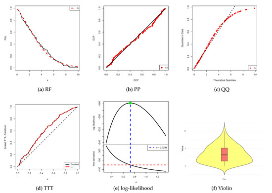
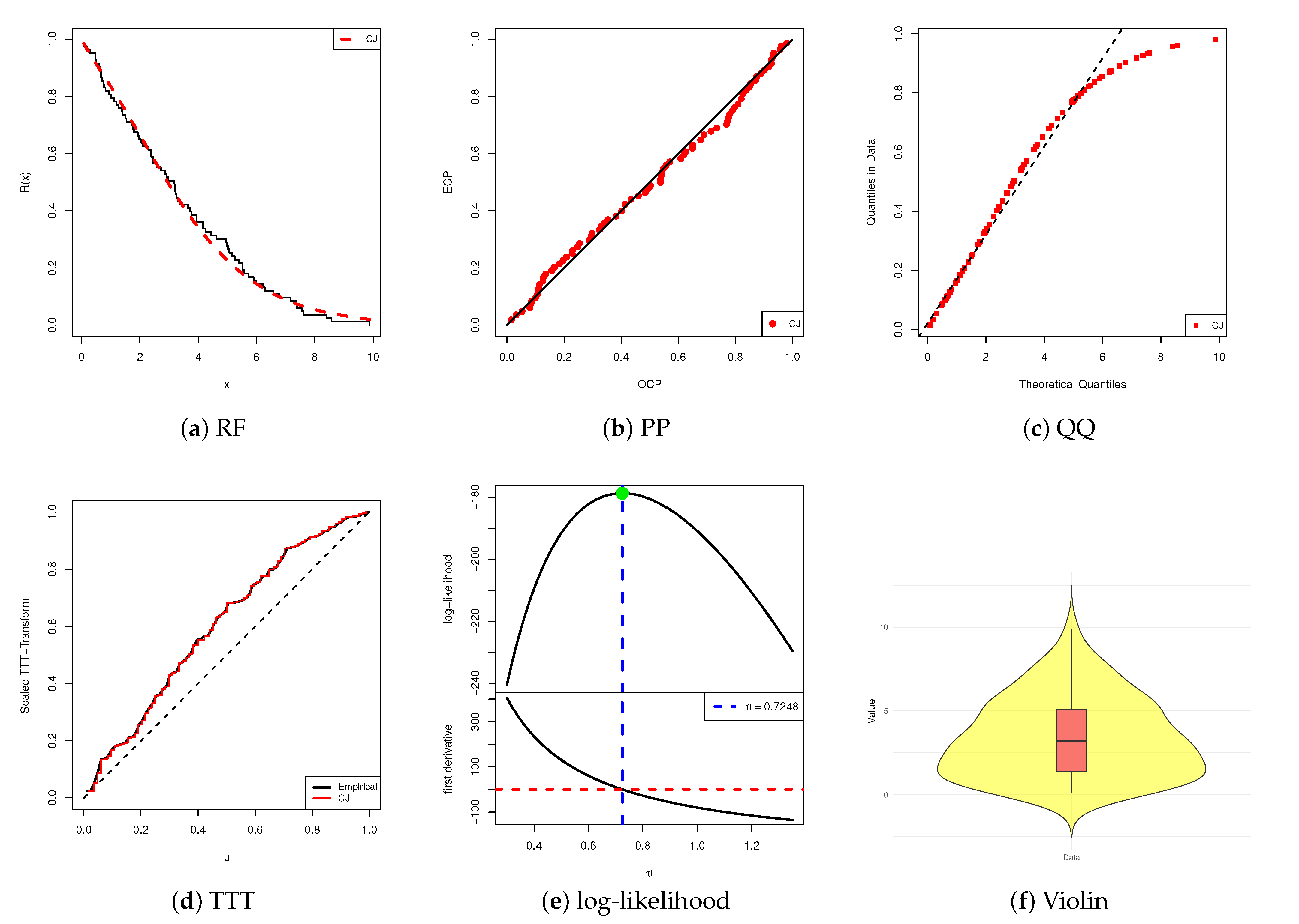
To visually evaluate the model fitting results, Figure 3 presents the RF plots, probability–probability (PP) and quantile–quantile (QQ) plots, the scaled total time on test (TTT) transform, the log-likelihood curve versus the normal equation, and a combined boxplot-within-violin plot. Based on the complete rainfall data summarized in Table 9, subplots in Figure 3a–c indicate a satisfactory fit of the CJ model, consistent with the numerical goodness-of-fit findings. Figure 3d shows that the data exhibit an increasing HRF, while Figure 3e confirms the existence and uniqueness of the MLE

\hat{ϑ}

. Accordingly,

\hat{ϑ}

is recommended as the initial value in subsequent estimation procedures. Finally, Figure 3f illustrates that the rainfall distribution is moderately right-skewed, with a wide spread and several high-value outliers, indicating notable variability in the dataset.

Figure 3. Fitting diagrams of the CJ model from the rainfall dataset.

From the full dataset of monthly rainfall, three artificial IT2-APC samples (with fixed

m = 43

and varying choices of

S

and threshold values

t_{i}, i = 1, 2

) are generated and summarized in Table 10. Since no prior knowledge of the CJ(

ϑ

) model is available for this dataset, an improper gamma prior with hyperparameters

a = b = 0.001

is employed to update

ϑ

. The frequentist point estimates of

ϑ

are used as initial values for running the proposed MCMC sampler. After discarding the first 10,000 iterations from a total of 50,000, the Bayesian point estimates and their associated credible interval estimates for

ϑ

,

R (x)

, and

h (x)

are obtained. For each configuration

S [i]

,

i = 1, 2, 3

, the point estimates (with their standard errors) and the corresponding 95% interval estimates (with interval lengths (ILs)) of

ϑ

,

R (x)

, and

h (x)

at

x = 0.1

are presented in Table 11. From Table 11, it is observed that the estimates of

ϑ

and

R (x)

, except for

h (x)

, obtained via the likelihood-based method are quite similar to those derived under the Bayesian framework. However, the Bayesian estimates generally outperform the frequentist ones in terms of smaller standard errors. Furthermore, both the 95% BCI and HPD interval results exhibit narrower widths than their 95% ACI-NA and ACI-NL counterparts, indicating improved precision.

Table 10. Different IT2-APC samples from the rainfall dataset.

Table 11. Estimates of

ϑ

,

R (x)

, and

h (x)

from rainfall data.

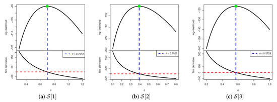
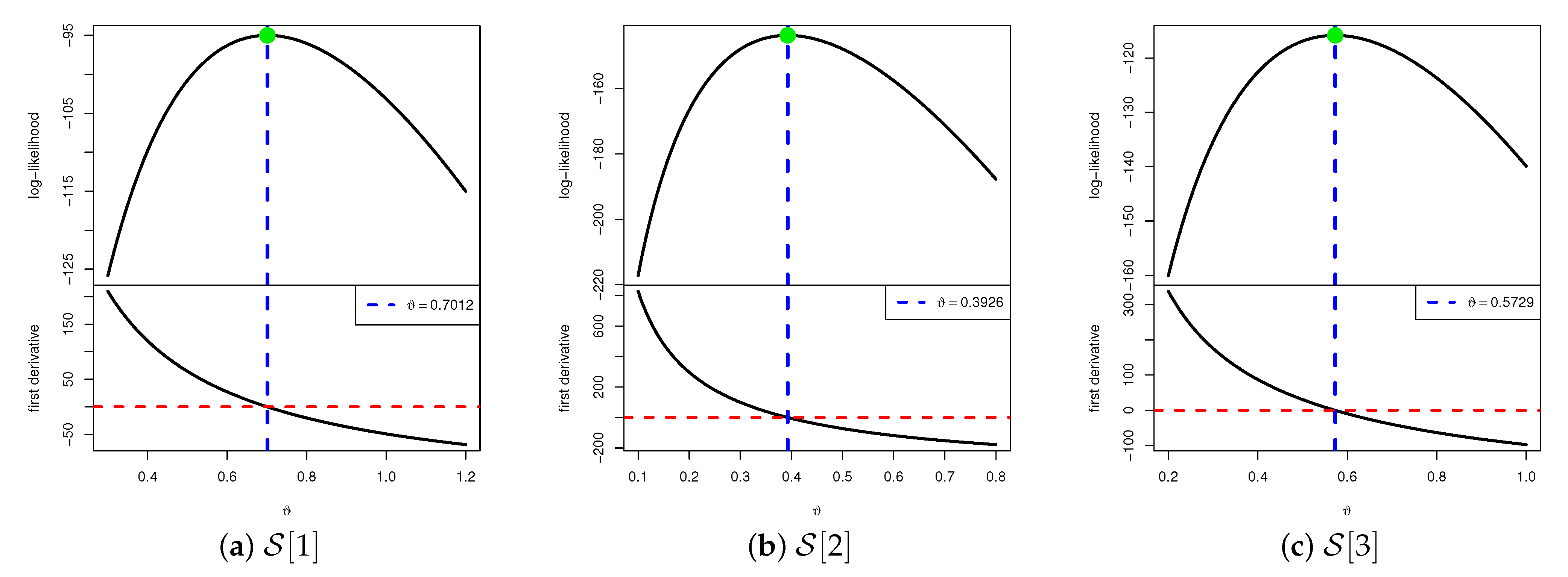
To demonstrate the existence and uniqueness of the fitted MLE

\hat{ϑ}

of

ϑ

, Figure 4 presents the log-likelihood curves along with their corresponding first derivative (score) functions for all samples

S [i]

,

i = 1, 2, 3

, under varying values of

ϑ

. The plots clearly show that the estimated MLE

\hat{ϑ}

exists and is unique for each sample configuration. These graphical results are consistent with the numerical findings reported in Table 11 and further justify the use of the estimated

\hat{ϑ}

values as initial guesses in subsequent Bayesian inference procedures.

Figure 4. Plots of log-likelihood/score functions of

ϑ

from the rainfall data.

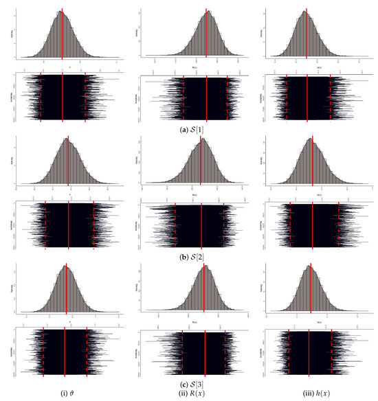
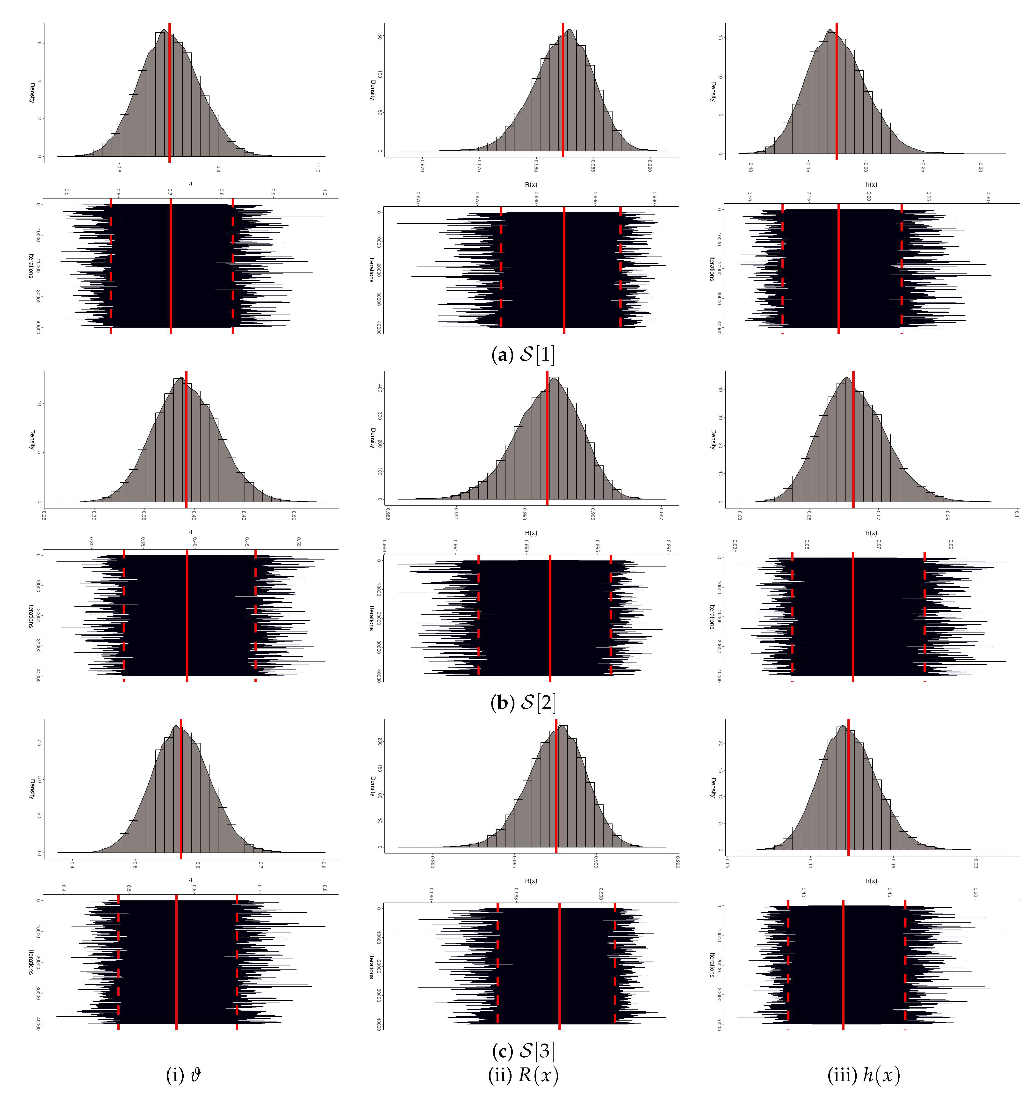
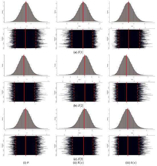
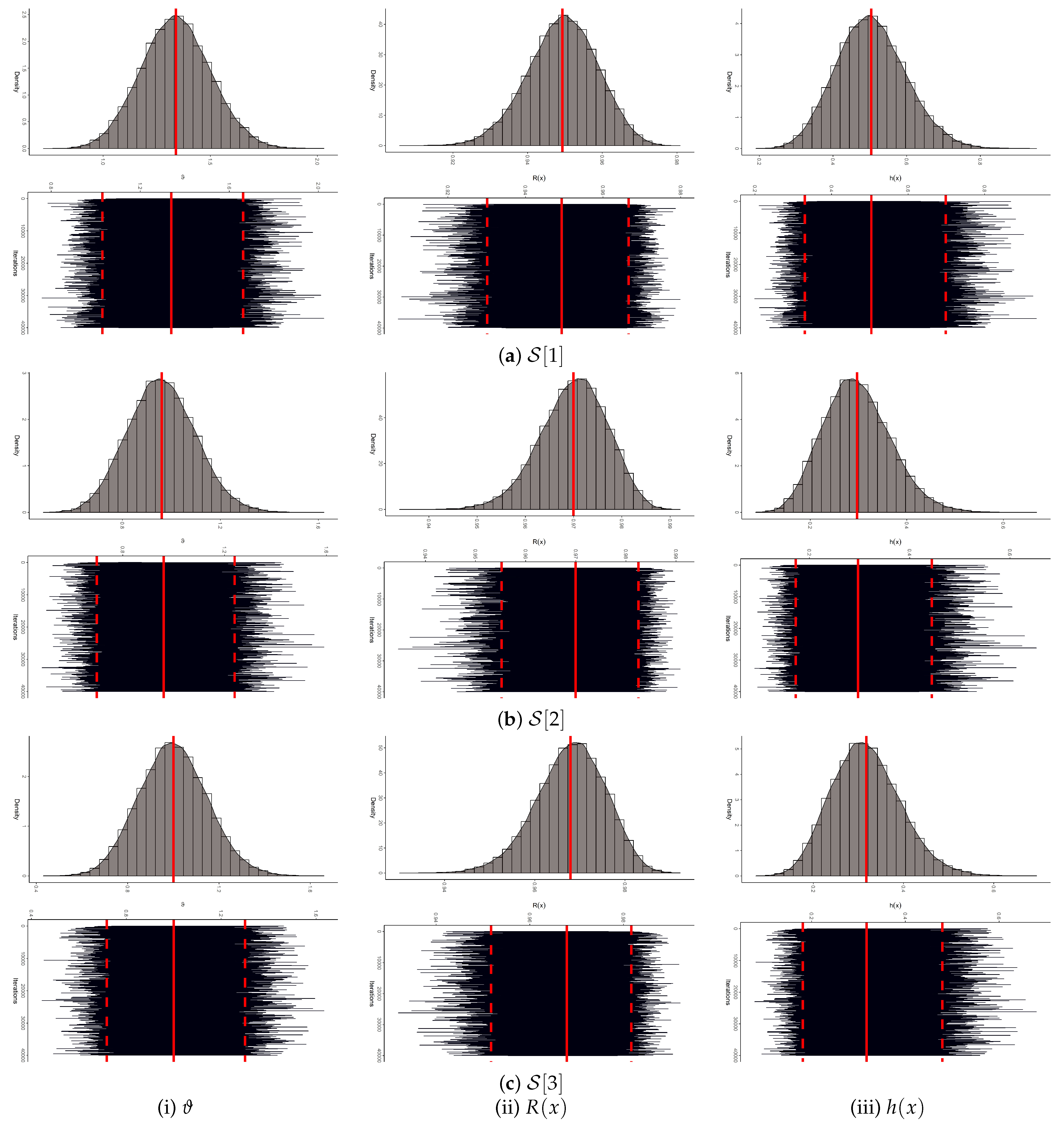
To assess the convergence behavior of the MCMC samples for

ϑ

,

R (x)

, and

h (x)

, both trace plots and posterior density plots for each parameter are presented in Figure 5. For clarity, the MCMC posterior mean and the 95% BCI bounds are indicated by solid and dashed red lines, respectively. Figure 5 shows that the generated Markov chains for

ϑ

,

R (x)

, and

h (x)

exhibit satisfactory convergence. Moreover, the posterior samples of

ϑ

are approximately symmetric, while those of

R (x)

and

h (x)

display negative and positive skewness, respectively. Using the remaining 40,000 post-burn-in MCMC iterations, various summary statistics for

ϑ

,

R (x)

, and

h (x)

were computed. These include the posterior mean, mode, quartiles

Q [i]

for

i = 1, 2, 3

, standard deviation (Std.D), and skewness (Sk.); see Table 12. All findings in Table 12 support the results reported in Table 11 and are visually confirmed in Figure 5.

Figure 5. The density (top) and trace (bottom) for 40,000 MCMC iterations of

ϑ

,

R (x)

, and

h (x)

from the rainfall dataset.

Table 12. Statistics for 40,000 MCMC iterations of

ϑ

,

R (x)

, and

h (x)

from rainfall data.

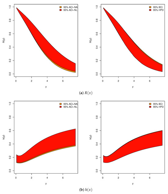
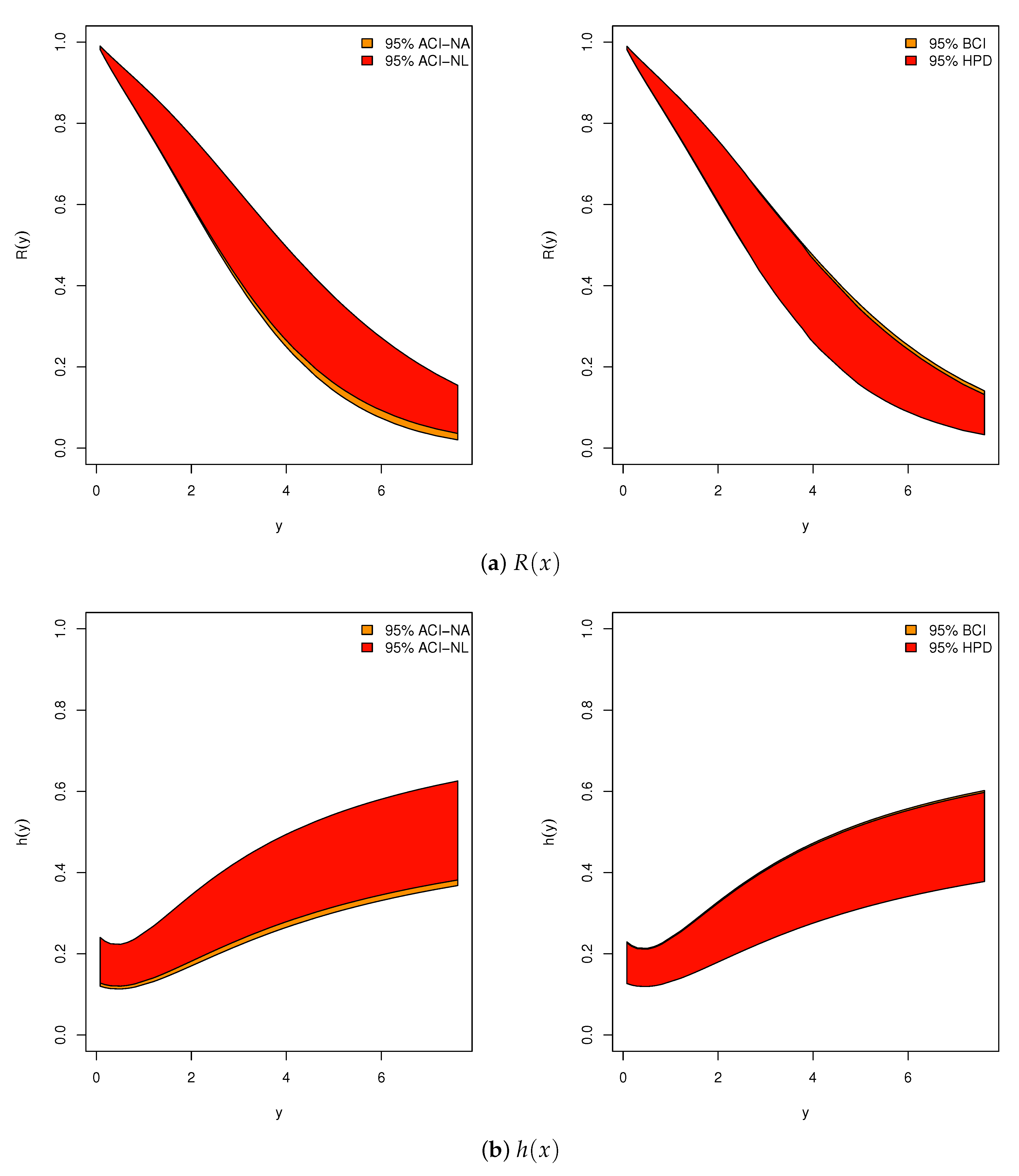
Figure 6 depicts the 95% ACI-NA/ACI-NL and BCI/HPD boundaries illustrating the performance of the reliability indices

R (x)

and

h (x)

over all data points in the

S [1]

sample from the rainfall dataset. The figure shows that the intervals for

R (x)

and

h (x)

obtained using the BCI (or HPD) methods have shorter ILs compared to those from the ACI-NA and ACI-NL methods, confirming the numerical findings reported in Table 11.

Figure 6. Plots for 95% IL results of

R (x)

and

h (x)

from rainfall data.

5.2. Engineering Application

This application analyzes the failure times of 18 electronic devices exhibiting a bathtub-shaped HRF, characterized by an initially high failure rate during early use, a plateau of relatively constant failure risk, and a subsequent increase due to aging and wear-out effects. To examine the applicability of the theoretical results for

ϑ

,

R (x)

, and

h (x)

in an engineering context, we analyze the complete failure time data for these devices. This dataset was first reported by Wang [21] and later revisited by Elshahhat and Abu El Azm [22]. To further demonstrate the suitability of the CJ distribution for this dataset, we compare our results with those of Elshahhat and Abu El Azm [22], who fitted the Nadarajah–Haghighi distribution to the same data. Their analysis yielded a KS statistic of

0.121

with a p-value of

0.9253

. In contrast, the CJ model achieves a smaller KS statistic of

0.1009

and a higher p-value of

0.9840

, indicating an improved fit. This comparison reinforces the effectiveness of the CJ distribution in modeling lifetime data for this application. For computational convenience, each failure time in the electronic devices dataset has been scaled by a factor of 100; see Table 13.

Table 13. Times to failure of 18 electronic devices.

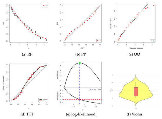
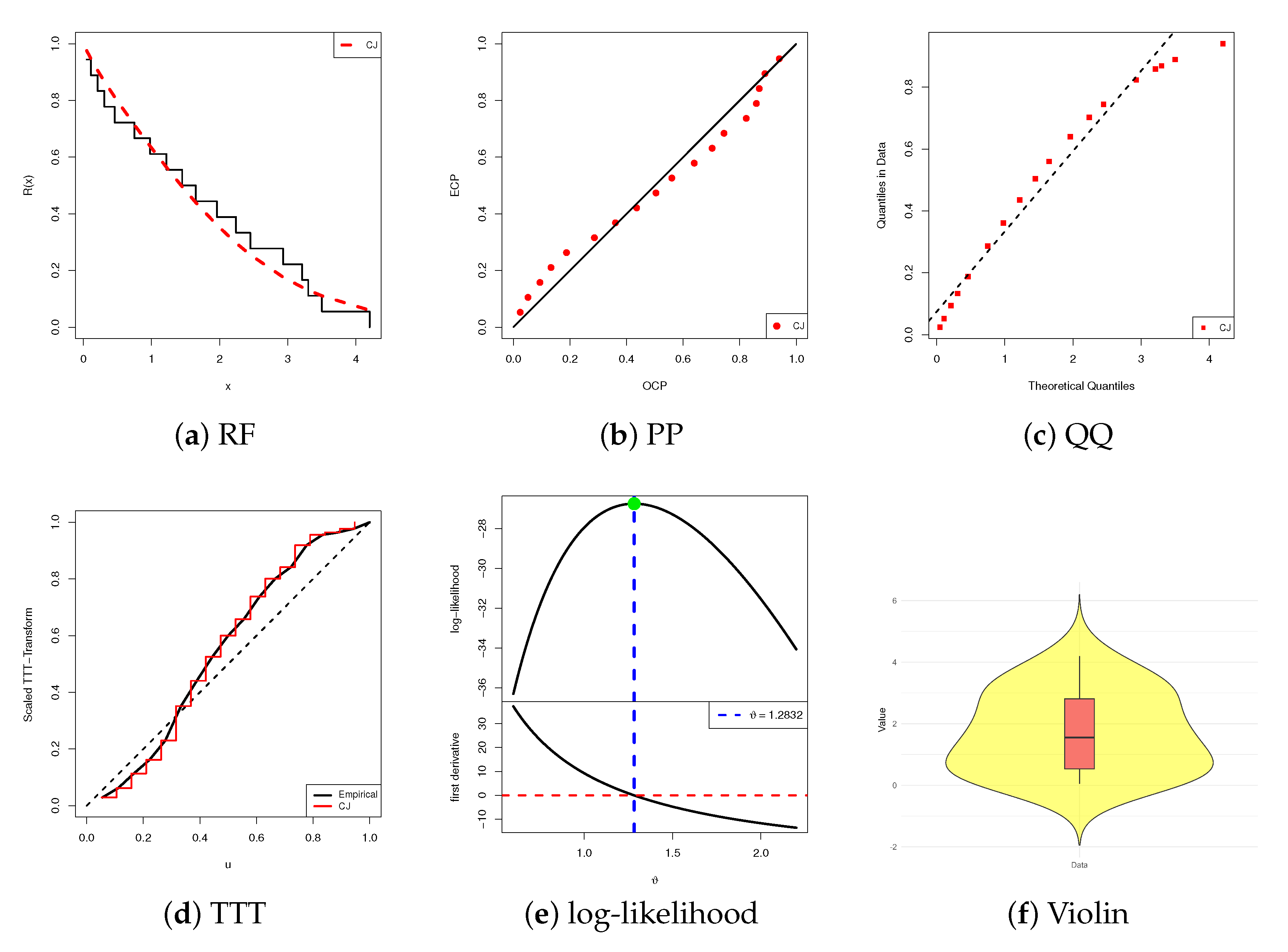
We now assess the adequacy of the CJ model before going to calculate the point and interval estimates of

ϑ

,

R (x)

, and

h (x)

. Based on Table 13, the MLE (Std.Er) of

ϑ

is 1.2832 (0.1981), and KS (p-value) is 0.1009 (0.9840). These findings indicate that the CJ model provides a satisfactory fit to the electronic devices data, supported by relatively narrow confidence intervals and a high p-value. To visually validate these results, Figure 7 presents the RF, PP, and QQ plots, the scaled TTT transform, the log-likelihood curve against the score function, and a combined boxplot-within-violin visualization. As shown in Figure 7a–c, the CJ model fits the electronic devices data well, consistent with the numerical results. Figure 7d confirms the presence of a bathtub-shaped HRF, while Figure 7e verifies the existence and uniqueness of the MLE

\hat{ϑ}

. We therefore recommend using

\hat{ϑ}

as the initial value in subsequent computations. Compared to the dataset analyzed in Section 5.1, Figure 7f reveals that the electronic devices dataset exhibits a symmetrical distribution with lower variability of failure times.

Figure 7. Fitting diagrams of the CJ model from the electronic devices dataset.

From the complete failure times of electronic devices, three IT2-APC samples are generated, each with a fixed sample size

m = 10

and varying configurations of the censoring scheme

S

and threshold parameters

t_{i}, i = 1, 2

, as summarized in Table 14. In the absence of prior information on the CJ(

ϑ

) model from the electronic devices data, an improper gamma prior with hyperparameters

a = b = 0.001

is employed for updating

ϑ

. The frequentist point estimates of

ϑ

are used as initial values for the proposed MCMC sampler. After discarding the first 10,000 iterations from a total of 50,000, Bayesian point and credible interval estimates for

ϑ

,

R (x)

, and

h (x)

are obtained.

Table 14. Various IT2-APC samples from the electronic devices dataset.

For each design

S [i]

,

i = 1, 2, 3

, Table 15 reports the point estimates (with standard errors) and the corresponding 95% credible and confidence intervals (with interval widths) of

ϑ

,

R (x)

, and

h (x)

at

x = 0.1

. The results show that the LF-based and Bayesian estimates of

ϑ

and

R (x)

, except for

h (x)

, are closely aligned. However, the Bayesian approach consistently yields estimates with smaller standard errors, demonstrating improved stability. Furthermore, the 95% BCI and HPD intervals are shorter than their ACI-NA and ACI-NL counterparts, confirming the superior precision of Bayesian inference in this setting.

Table 15. Estimates of

ϑ

,

R (x)

, and

h (x)

from electronic devices data.

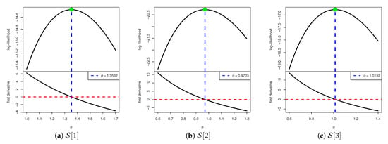
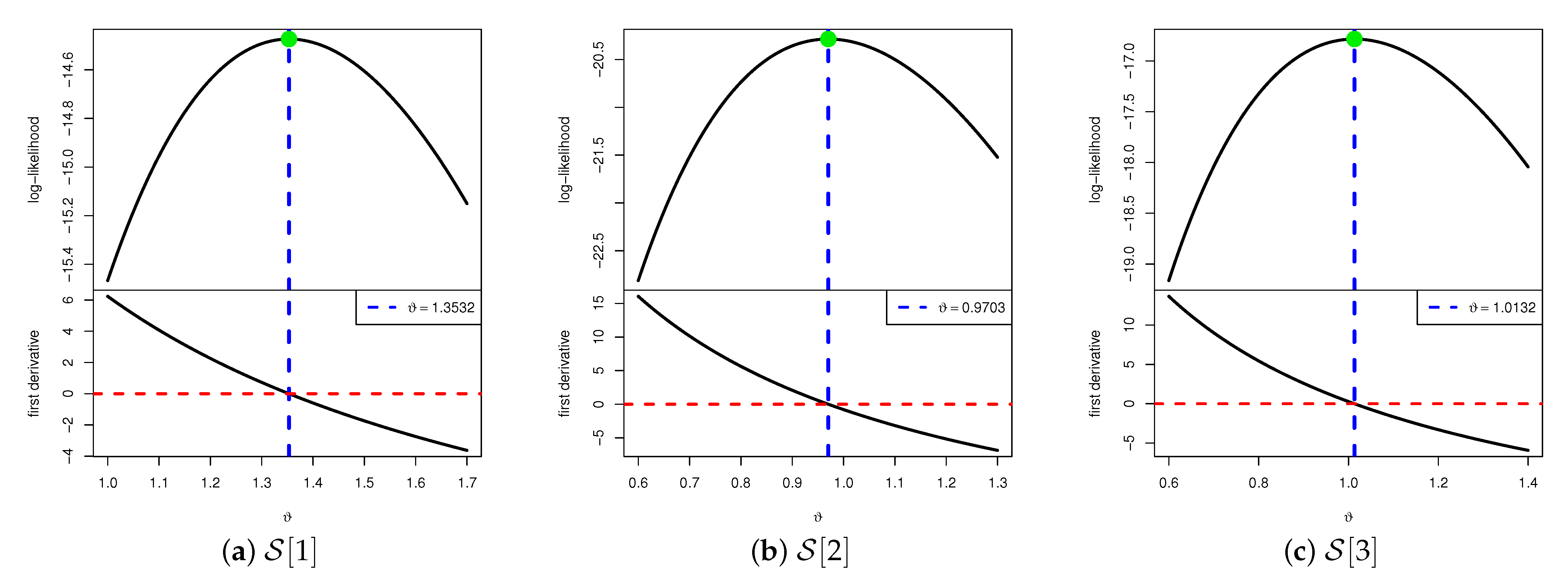
To confirm the existence and uniqueness of the estimated MLE

\hat{ϑ}

, Figure 8 displays the log-LFs together with their associated score functions for each sample configuration

S [i]

,

i = 1, 2, 3

, evaluated under different values of

ϑ

. The plots distinctly reveal that a unique maximum of the LF exists for every case considered, thereby ensuring the well-posedness of the estimation procedure. These graphical findings are consistent with the numerical evidence provided in Table 15 and further justify the use of

\hat{ϑ}

as a reliable initial value in the Bayesian estimation framework.

Figure 8. Plots of log-likelihood/score functions of

ϑ

from electronic devices data.

The convergence behavior of the MCMC samples for

ϑ

,

R (x)

, and

h (x)

is evaluated using trace plots and posterior density plots, as shown in Figure 9. For reference, the posterior mean and corresponding 95% BCI limits are indicated by red solid and dashed lines, respectively. Visual inspection of these plots suggests satisfactory mixing and no evident convergence issues for the Markov chains of all parameters. The posterior distribution of

ϑ

is approximately symmetric, while those of

R (x)

and

h (x)

exhibit left and right skewness, respectively. Using the 40,000 post-burn-in MCMC iterations, a comprehensive set of posterior summary statistics for

ϑ

,

R (x)

, and

h (x)

has been computed. The results in Table 16 closely align with those in Table 15 and corroborate the graphical diagnostics in Figure 9, confirming the reliability and consistency of the Bayesian estimates.

Figure 9. The density (top) and trace (bottom) for 40,000 MCMC iterations of

ϑ

,

R (x)

, and

h (x)

from the electronic devices dataset.

Table 16. Statistics for 40,000 MCMC iterations of

ϑ

,

R (x)

, and

h (x)

from electronic devices data.

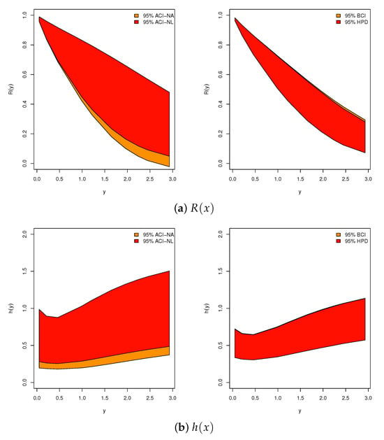
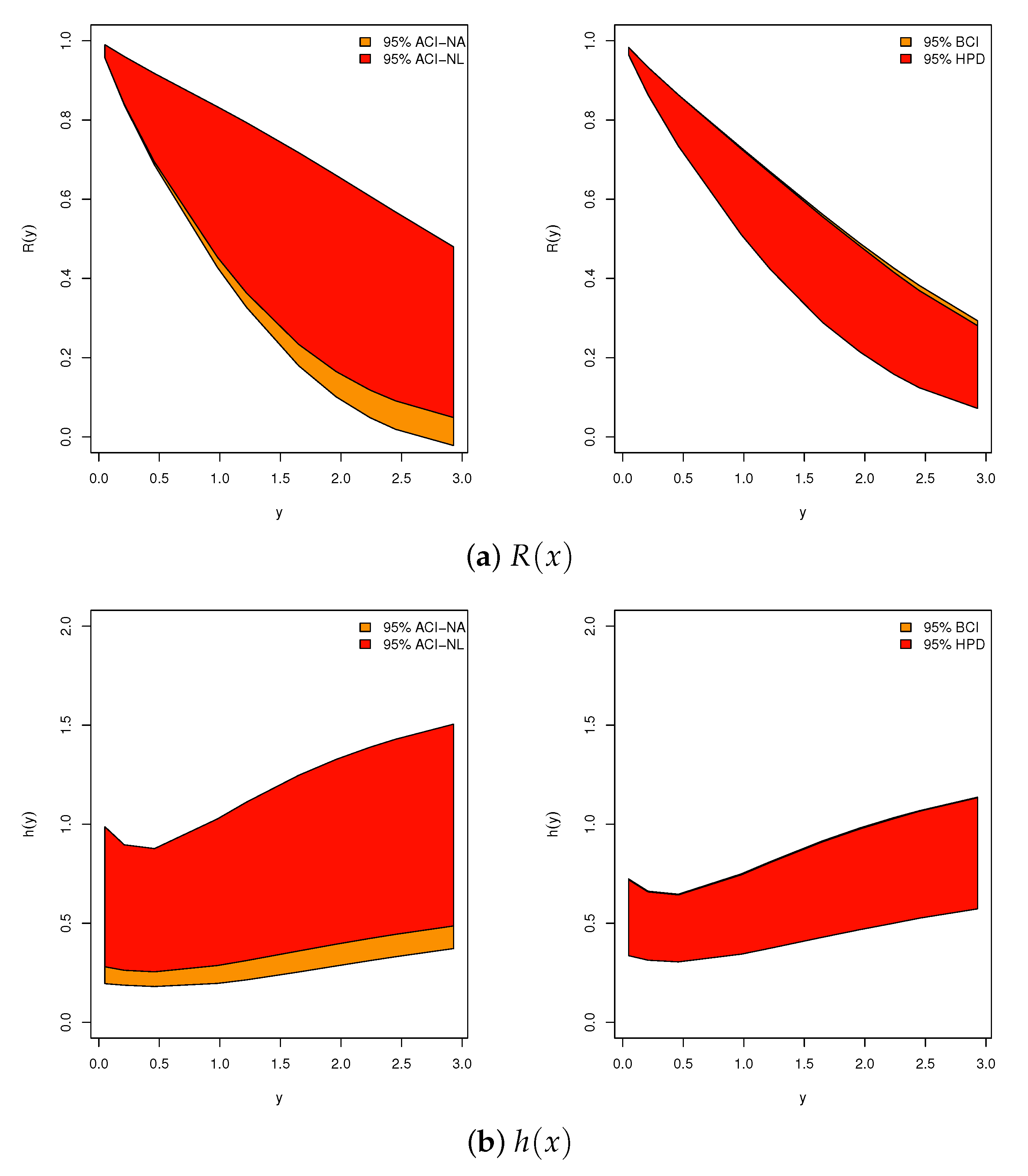
Figure 10 displays the 95% confidence and credible interval bounds for the reliability measures

R (x)

and

h (x)

, computed using the ACI-NA, ACI-NL, and BCI/HPD methods for the electronic devices dataset sample

S [1]

. The intervals obtained via the BCI (or HPD) approach are noticeably narrower than those produced by the classical ACI-NA and ACI-NL methods. This finding is consistent with the numerical results in Table 15 and further highlights the advantage of the Bayesian framework in delivering more precise inference through shorter interval lengths.

Figure 10. Plots for 95% IL results of

R (x)

and

h (x)

from electronic devices data.

As a result, the analyses of samples generated under the improved Type-II adaptive progressive censoring scheme—applied to both the rainfall and electronic device datasets—provide a comprehensive assessment of the CJ lifetime model. These findings corroborate the simulation results and further demonstrate the practical utility of the proposed methodology in engineering and physical sciences applications.

6. Conclusions

This study introduces a comprehensive reliability framework based on the CJ lifetime distribution combined with an adaptive progressive Type-II censoring plan. The proposed censoring strategy enhances flexibility and efficiency in data collection for life-testing experiments. Maximum likelihood and Bayesian estimators were derived for the CJ parameter and key reliability metrics, including the reliability function and hazard rate function. Approximate confidence intervals were obtained using the observed Fisher information matrix and the delta method. To address the intractability of the likelihood, Bayesian estimation was performed under independent gamma priors and a squared-error loss function. A Metropolis–Hastings sampler was developed to generate posterior samples, enabling the computation of Bayesian estimates along with credible and highest posterior density intervals. Extensive simulation studies verified the consistency and efficiency of the proposed estimators across diverse censoring scenarios. Two real-world datasets—rainfall measurements and mechanical failure times—were analyzed to demonstrate the model’s practical applicability. In both cases, the CJ distribution under the proposed scheme achieved superior fit and inference compared to traditional approaches. Overall, this work provides a flexible and computationally efficient inferential framework for analyzing censored lifetime data using the CJ distribution, with significant relevance to environmental, industrial, and engineering reliability studies.

Author Contributions

Methodology, H.S.M., O.E.A.-K. and A.E.; Funding acquisition, H.S.M.; Software, A.E.; Supervision, O.E.A.-K.; Writing—original draft, H.S.M., O.E.A.-K. and A.E.; Writing—review and editing, H.S.M. and A.E. All authors have read and agreed to the published version of the manuscript.

Funding

This research was funded by Princess Nourah bint Abdulrahman University Researchers Supporting Project number (PNURSP2025R175), Princess Nourah bint Abdulrahman University, Riyadh, Saudi Arabia.

Data Availability Statement

The authors confirm that the data supporting the findings of this study are available within the article.

Conflicts of Interest

The authors declare no conflicts of interest.

List of Abbreviations

Abbreviation	Meaning
ACI	Asymptotic Confidence Interval
ACI-NA	Asymptotic Confidence Interval using Normal Approximation
ACI-NL	Asymptotic Confidence Interval using Log-Transformed Method
BCI	Bayesian Credible Interval
CDF	Cumulative Distribution Function
CJ	Chris–Jerry
CP	Coverage Probability
FI	Fisher Information
HPD	Highest Posterior Density
IL	Interval Length
IT2-APC	Improved Type-II Adaptive Progressive Censoring
log-MLE	Log-Transformed Maximum Likelihood Estimator
LF	Likelihood Function
PDF	Probability Density Function
KS	Kolmogorov–Smirnov (test)
NR	Newton–Raphson
M-H	Metropolis–Hastings
MCMC	Markov Chain Monte Carlo
MLE	Maximum Likelihood Estimator
MPE	Mean Point Estimate
MRAB	Mean Relative Absolute Bias
RMSE	Root Mean Squared Error
Sk.	Skewness
Std.D	Standard Deviation
SEL	Squared-Error Loss
T1-PHC	Type-I Progressive Hybrid Censoring
T2-APC	Type-II Adaptive Progressive Censoring
T2-PC	Type-II Progressive Censoring
T2-C	Type-II Censoring
TTT	Total Time on Test
VC	Variance-Covariance

References

Onyekwere, C.K.; Obulezi, O.J. Chris-Jerry distribution and its applications. Asian J. Probab. Stat. 2022, 20, 16–30. [Google Scholar] [CrossRef] [Scilit]
Alotaibi, R.; Rezk, H.; Elshahhat, A. Evaluations of Chris-Jerry Data Using Generalized Progressive Hybrid Strategy and Its Engineering Applications. CMES Comput. Model. Eng. Sci. 2024, 140, 3073–3103. [Google Scholar] [CrossRef] [Scilit]
Balakrishnan, N.; Cramer, E. The Art of Progressive Censoring; Springer: Birkhäuser, NY, USA, 2014. [Google Scholar]
Kundu, D.; Joarder, A. Analysis of Type-II progressively hybrid censored data. Comput. Stat. Data Anal. 2006, 50, 2509–2528. [Google Scholar] [CrossRef] [Scilit]
Ng, H.K.T.; Kundu, D.; Chan, P.S. Statistical Analysis of Exponential Lifetimes under an Adaptive Type-II Progressive Censoring Scheme. Nav. Res. Logist. 2009, 56, 687–698. [Google Scholar] [CrossRef] [Scilit]
Yan, W.; Li, P.; Yu, Y. Statistical inference for the reliability of Burr-XII distribution under improved adaptive Type-II progressive censoring. Appl. Math. Model. 2021, 95, 38–52. [Google Scholar] [CrossRef] [Scilit]
Bain, L.J.; Engelhardt, M. Statistical Analysis of Reliability and Life-Testing Models, 2nd ed.; Marcel Dekker: New York, NY, USA, 1991. [Google Scholar]
Nassar, M.; Elshahhat, A. Estimation procedures and optimal censoring schemes for an improved adaptive progressively type-II censored Weibull distribution. J. Appl. Stat. 2024, 51, 1664–1688. [Google Scholar] [CrossRef] [Scilit] [PubMed]
Asadi, S.; Panahi, H.; Anwar, S.; Lone, S.A. Reliability Estimation of Burr Type III Distribution under Improved Adaptive Progressive Censoring with Application to Surface Coating. Maint. Reliab. Niezawodn. 2023, 25, 163054. [Google Scholar] [CrossRef] [Scilit]
El-Sherpieny, E.S.A.; Elshahhat, A.; Abdallah, N.M. Statistical analysis of improved Type-II adaptive progressive hybrid censored NH data. Sankhya A 2024, 86, 721–754. [Google Scholar] [CrossRef] [Scilit]
Alqasem, O.A.; Elshahhat, A. Reliability Analysis of the Newly Power Half-Normal Model via Improving Adaptive Progressive Type II Censoring and Its Applications. Qual. Reliab. Eng. Int. 2025. early view. [Google Scholar] [CrossRef] [Scilit]
Henningsen, A.; Toomet, O. maxLik: A package for maximum likelihood estimation in R. Comput. Stat. 2011, 26, 443–458. [Google Scholar] [CrossRef] [Scilit]
Plummer, M.; Best, N.; Cowles, K.; Vines, K. CODA: Convergence diagnosis and output analysis for MCMC. R News 2006, 6, 7–11. [Google Scholar]
Greene, W.H. Econometric Analysis, 4th ed.; Prentice-Hall: New York, NY, USA, 2000. [Google Scholar]
Meeker, W.Q.; Escobar, L.A. Statistical Methods for Reliability Data; John Wiley and Sons: New York, NY, USA, 2014. [Google Scholar]
Gelman, A.; Carlin, J.B.; Stern, H.S.; Rubin, D.B. Bayesian Data Analysis, 2nd ed.; Chapman and Hall/CRC: Boca Raton, FL, USA, 2004. [Google Scholar]
Kundu, D. Bayesian inference and life testing plan for the Weibull distribution in presence of progressive censoring. Technometrics 2008, 50, 144–154. [Google Scholar] [CrossRef] [Scilit]
Jodrá, P.; Jiménez-Gamero, M.D.; Alba-Fernández, M.V. On the Muth distribution. Math. Model. Anal. 2015, 20, 291–310. [Google Scholar] [CrossRef] [Scilit]
Alotaibi, R.; Nassar, M.; Elshahhat, A. Data analysis with applications in physics and engineering using XLindley model with improved adaptive Type-II progressively censored samples. Heliyon 2024, 10, e33598. [Google Scholar] [CrossRef] [Scilit] [PubMed]
Alotaibi, R.; Nassar, M.; Elshahhat, A. Rainfall data modeling using improved adaptive type-II progressively censored Weibull-exponential samples. Sci. Rep. 2024, 14, 30484. [Google Scholar] [CrossRef] [Scilit] [PubMed]
Wang, F.K. A new model with bathtub-shaped failure rate using an additive Burr XII distribution. Reliab. Eng. Syst. Saf. 2000, 70, 305–312. [Google Scholar] [CrossRef] [Scilit]
Elshahhat, A.; Abu El Azm, W.S. Statistical reliability analysis of electronic devices using generalized progressively hybrid censoring plan. Qual. Reliab. Eng. Int. 2022, 38, 1112–1130. [Google Scholar] [CrossRef] [Scilit]

Figure 1. The log-LF curve versus its score function curve.

Figure 2. The likelihood, prior, and posterior density shapes.

Figure 3. Fitting diagrams of the CJ model from the rainfall dataset.

Figure 4. Plots of log-likelihood/score functions of

ϑ

from the rainfall data.

Figure 4. Plots of log-likelihood/score functions of

ϑ

from the rainfall data.

Figure 5. The density (top) and trace (bottom) for 40,000 MCMC iterations of

ϑ

,

R (x)

, and

h (x)

from the rainfall dataset.

Figure 5. The density (top) and trace (bottom) for 40,000 MCMC iterations of

ϑ

,

R (x)

, and

h (x)

from the rainfall dataset.

Figure 6. Plots for 95% IL results of

R (x)

and

h (x)

from rainfall data.

Figure 6. Plots for 95% IL results of

R (x)

and

h (x)

from rainfall data.

Figure 7. Fitting diagrams of the CJ model from the electronic devices dataset.

Figure 8. Plots of log-likelihood/score functions of

ϑ

from electronic devices data.

Figure 8. Plots of log-likelihood/score functions of

ϑ

from electronic devices data.

Figure 9. The density (top) and trace (bottom) for 40,000 MCMC iterations of

ϑ

,

R (x)

, and

h (x)

from the electronic devices dataset.

Figure 9. The density (top) and trace (bottom) for 40,000 MCMC iterations of

ϑ

,

R (x)

, and

h (x)

from the electronic devices dataset.

Figure 10. Plots for 95% IL results of

R (x)

and

h (x)

from electronic devices data.

Figure 10. Plots for 95% IL results of

R (x)

and

h (x)

from electronic devices data.

Table 1. Options of

A, B, T^{★}, S^{★}

and

(y_{i}, S_{i})

.

Table 1. Options of

A, B, T^{★}, S^{★}

and

(y_{i}, S_{i})

.

Case	A	B	$S^{★}$	$T^{★}$	${y_{i}, S_{i}}$
1	$m - 1$	m	$S_{m}$	$y_{m}$	${(y_{1}, S_{1}), \dots, (y_{m - 1}, S_{m - 1}), (y_{m}, S^{★})}$
2	$d_{1}$	m	$n - m - \sum_{i = 1}^{d_{1}} S_{i}$	$y_{m}$	${(y_{1}, S_{1}), \dots, (y_{d_{1}}, S_{d_{1}}), (y_{j_{1} + 1}, 0), \dots, (y_{m - 1}, 0), (y_{m}, S^{★})}$
3	$d_{1}$	$d_{2}$	$n - d_{2} - \sum_{i = 1}^{d_{1}} S_{i}$	$t_{2}$	${(y_{1}, S_{1}), \dots, (y_{d_{1}}, S_{d_{1}}), (y_{d_{1} + 1}, 0), \dots, (y_{d_{2} - 1}, 0), (y_{d_{2}}, 0)}$

Table 2. Different T2-PC designs in Monte Carlo simulations.

Test↓ $(n, m) \to$	(30,10)	Test↓	(30,20)	Test↓	(50,20)	Test↓	(50,40)	Test↓	(80,30)	Test↓	(80,60)
A1[1]	(5⁴,0⁶)	A1[4]	(5²,0¹⁸)	A2[1]	(5⁶,0¹⁴)	A2[4]	(5²,0³⁸)	A3[1]	(5¹⁰,0²⁰)	A3[4]	(5⁴,0⁵⁶)
B1[2]	(0³,5⁴,0³)	B1[5]	(0⁹,5²,0⁹)	B2[2]	(0⁷,5⁶,0⁷)	B2[5]	(0¹⁹,5²,0¹⁹)	B3[2]	(0¹⁰,5¹⁰,0¹⁰)	B3[5]	(0²⁸,5⁴,0²⁸)
C1[3]	(0⁶,5⁴)	C1[6]	(0¹⁸,5²)	C2[3]	(0¹⁴,5⁶)	C2[6]	(0³⁸,5²)	C3[3]	(0²⁰,5¹⁰)	C3[6]	(0⁵⁶,5⁴)

Table 9. Monthly total rainfall (in mm) in the state of New South Wales.

Table 10. Different IT2-APC samples from the rainfall dataset.

Sample	$S$	$t_{1} (d_{1})$	$t_{2} (d_{2})$	$S^{★}$	$T^{★}$	Data
$S$ [1]	$(5^{10}, 0^{33})$	7.65(43)	7.75(43)	0	7.61	0.08, 0.18, 0.30, 0.51, 0.64, 0.66, 0.69, 0.77, 0.82, 1.20,
						1.27, 1.40, 1.54, 1.73, 1.97, 2.11, 2.38, 2.38, 2.45, 2.45,
						2.57, 2.86, 3.18, 3.31, 3.65, 3.72, 3.77, 3.94, 4.16, 4.63,
						4.95, 5.02, 5.07, 5.16, 5.25, 5.52, 5.72, 5.90, 6.28, 6.58,
						6.79, 7.16, 7.61
$S$ [2]	$(0^{16}, 5^{10}, 0^{17})$	3.20(25)	8.50(43)	25	8.40	0.08, 0.08, 0.18, 0.30, 0.47, 0.48, 0.51, 0.59, 0.64, 0.66,
						0.67, 0.69, 0.76, 0.77, 0.82, 0.95, 1.01, 1.27, 1.40, 1.54,
						1.73, 1.77, 2.11, 3.18, 3.19, 3.20, 3.22, 3.25, 3.39, 3.94,
						4.16, 4.95, 4.99, 5.39, 5.52, 5.58, 5.72, 5.90, 5.97, 6.58,
						7.37, 7.55, 8.40
$S$ [3]	$(0^{33}, 5^{10})$	3.30(37)	3.95(40)	33	3.95	0.08, 0.08, 0.18, 0.30, 0.47, 0.48, 0.51, 0.59, 0.64, 0.66,
						0.67, 0.69, 0.76, 0.77, 0.82, 0.95, 1.01, 1.12, 1.20, 1.27,
						1.39, 1.40, 1.50, 1.54, 1.73, 1.77, 1.79, 1.94, 1.97, 2.04,
						2.11, 2.27, 2.38, 2.38, 2.57, 2.97, 3.20, 3.39, 3.77, 3.94

Table 11. Estimates of

ϑ

,

R (x)

, and

h (x)

from rainfall data.

Table 11. Estimates of

ϑ

,

R (x)

, and

h (x)

from rainfall data.

Sample	Par.	MLE		MCMC		ACI-NA			BCI
						ACI-NL			HPD
		Est.	Std.Er	Est.	Std.Er	Low.	Upp.	IL	Low.	Upp.	IL
$S$ [1]	$ϑ$	0.7012	0.0658	0.7009	0.0604	0.5723	0.8300	0.2578	0.5855	0.8212	0.2357
						0.5834	0.8426	0.2592	0.5815	0.8165	0.2350
	$R (x)$	0.9410	0.0028	0.9823	0.0026	0.9355	0.9465	0.0111	0.9770	0.9871	0.0101
						0.9355	0.9465	0.0111	0.9772	0.9873	0.0100
	$h (x)$	0.7001	0.0279	0.1745	0.0256	0.6455	0.7547	0.1092	0.1274	0.2272	0.0998
						0.6476	0.7569	0.1093	0.1259	0.2250	0.0991
$S$ [2]	$ϑ$	0.3926	0.0344	0.3922	0.0325	0.3251	0.4601	0.1350	0.3312	0.4582	0.1270
						0.3305	0.4662	0.1357	0.3311	0.4580	0.1269
	$R (x)$	0.9410	0.0010	0.9937	0.0010	0.9390	0.9430	0.0040	0.9916	0.9954	0.0037
						0.9390	0.9430	0.0040	0.9918	0.9955	0.0037
	$h (x)$	0.7001	0.0099	0.0627	0.0094	0.6806	0.7196	0.0390	0.0459	0.0827	0.0368
						0.6809	0.7199	0.0390	0.0447	0.0812	0.0365
$S$ [3]	$ϑ$	0.5730	0.0519	0.5725	0.0463	0.4713	0.6746	0.2033	0.4835	0.6653	0.1818
						0.4798	0.6842	0.2044	0.4816	0.6629	0.1812
	$R (x)$	0.9410	0.0020	0.9875	0.0018	0.9371	0.9448	0.0077	0.9839	0.9908	0.0069
						0.9371	0.9449	0.0077	0.9841	0.9910	0.0069
	$h (x)$	0.7001	0.0194	0.1230	0.0174	0.6621	0.7382	0.0761	0.0909	0.1590	0.0680
						0.6631	0.7392	0.0761	0.0892	0.1567	0.0675

Table 12. Statistics for 40,000 MCMC iterations of

ϑ

,

R (x)

, and

h (x)

from rainfall data.

Table 12. Statistics for 40,000 MCMC iterations of

ϑ

,

R (x)

, and

h (x)

from rainfall data.

Sample	Par.	Mean	Mode	$Q [1]$	$Q [2]$	$Q [3]$	Std.D	Sk.
$S$ [1]	$ϑ$	0.70092	0.69672	0.65936	0.69924	0.74095	0.06040	0.12631
	$R (x)$	0.98233	0.98257	0.98065	0.98246	0.98414	0.00260	−0.27531
	$h (x)$	0.17448	0.17206	0.15654	0.17312	0.19107	0.02563	0.27821
$S$ [2]	$ϑ$	0.39219	0.40372	0.36988	0.39091	0.41402	0.03247	0.14476
	$R (x)$	0.99366	0.99335	0.99303	0.99372	0.99433	0.00095	−0.32334
	$h (x)$	0.06274	0.06583	0.05616	0.06209	0.06889	0.00941	0.32237
$S$ [3]	$ϑ$	0.57247	0.55790	0.54104	0.57156	0.60335	0.04631	0.10383
	$R (x)$	0.98755	0.98814	0.98640	0.98763	0.98877	0.00176	−0.26050
	$h (x)$	0.12296	0.11711	0.11097	0.12218	0.13427	0.01735	0.26139

Table 13. Times to failure of 18 electronic devices.

Table 14. Various IT2-APC samples from the electronic devices dataset.

Sample	S	$t_{1} (d_{1})$	$t_{2} (d_{2})$	$S^{★}$	$T^{★}$	Data
$S$ [1]	$(2^{4}, 0^{6})$	2.95(10)	3.10(10)	0	2.93	0.05, 0.21, 0.46, 0.98, 1.22, 1.65, 1.96, 2.24, 2.45, 2.93
$S$ [2]	$(0^{3}, 2^{4}, 0^{3})$	0.85(5)	3.25(10)	4	3.21	0.05, 0.11, 0.21, 0.31, 0.75, 0.98, 1.45, 2.24, 2.93, 3.21
$S$ [3]	$(0^{6}, 2^{4})$	1.25(7)	2.00(8)	8	2.00	0.05, 0.11, 0.21, 0.31, 0.46, 0.75, 0.98, 1.96

Table 15. Estimates of

ϑ

,

R (x)

, and

h (x)

from electronic devices data.

Table 15. Estimates of

ϑ

,

R (x)

, and

h (x)

from electronic devices data.

Sample	Par.	MLE		MCMC		ACI-NA			BCI
						ACI-NL			HPD
		Est.	Std.Er	Est.	Std.Er	Low.	Upp.	IL	Low.	Upp.	IL
$S$ [1]	$ϑ$	1.3532	0.2762	1.3395	0.1620	0.8120	1.8945	1.0825	1.0301	1.6621	0.6320
						0.9071	2.0187	1.1116	1.0380	1.6696	0.6315
	$R (x)$	0.9410	0.0161	0.9493	0.0094	0.9095	0.9725	0.0630	0.9301	0.9666	0.0365
						0.9100	0.9730	0.0630	0.9305	0.9669	0.0364
	$h (x)$	0.7001	0.1620	0.5038	0.0944	0.3827	1.0176	0.6349	0.3302	0.6983	0.3681
						0.4449	1.1018	0.6568	0.3271	0.6947	0.3675
$S$ [2]	$ϑ$	0.9703	0.1905	0.9604	0.1383	0.5969	1.3437	0.7468	0.6982	1.2395	0.5413
						0.6604	1.4257	0.7653	0.6866	1.2243	0.5376
	$R (x)$	0.9410	0.0097	0.9700	0.0070	0.9220	0.9600	0.0380	0.9552	0.9825	0.0273
						0.9222	0.9602	0.0380	0.9564	0.9833	0.0269
	$h (x)$	0.7001	0.0963	0.2970	0.0695	0.5115	0.8888	0.3773	0.1727	0.4441	0.2714
						0.5348	0.9166	0.3819	0.1651	0.4324	0.2673
$S$ [3]	$ϑ$	1.0132	0.2203	1.0000	0.1493	0.5814	1.4450	0.8636	0.7180	1.3005	0.5825
						0.6616	1.5516	0.8900	0.7068	1.2879	0.5811
	$R (x)$	0.9410	0.0114	0.9679	0.0077	0.9186	0.9634	0.0448	0.9517	0.9816	0.0299
						0.9189	0.9637	0.0448	0.9530	0.9826	0.0296
	$h (x)$	0.7001	0.1137	0.3174	0.0763	0.4773	0.9230	0.4457	0.1811	0.4789	0.2978
						0.5093	0.9625	0.4533	0.1722	0.4664	0.2943

Table 16. Statistics for 40,000 MCMC iterations of

ϑ

,

R (x)

, and

h (x)

from electronic devices data.

Table 16. Statistics for 40,000 MCMC iterations of

ϑ

,

R (x)

, and

h (x)

from electronic devices data.

Sample	Par.	Mean	Mode	$Q [1]$	$Q [2]$	$Q [3]$	Std.D	Sk.
$S$ [1]	$ϑ$	1.33950	1.18867	1.22930	1.33764	1.44701	0.16145	0.08795
	$R (x)$	0.94930	0.94559	0.94318	0.94961	0.95579	0.00934	−0.20724
	$h (x)$	0.50385	0.41556	0.43829	0.50047	0.56533	0.09420	0.22880
$S$ [2]	$ϑ$	0.96044	0.86222	0.86546	0.95729	1.05259	0.13799	0.13274
	$R (x)$	0.96996	0.97504	0.96543	0.97036	0.97489	0.00698	−0.32834
	$h (x)$	0.29704	0.24649	0.24803	0.29297	0.34195	0.06941	0.34114
$S$ [3]	$ϑ$	1.00002	0.92869	0.89792	0.99764	1.09871	0.14867	0.11563
	$R (x)$	0.96791	0.97179	0.96298	0.96830	0.97331	0.00766	−0.31429
	$h (x)$	0.31742	0.27873	0.26365	0.31343	0.36644	0.07621	0.32884

Disclaimer/Publisher’s Note: The statements, opinions and data contained in all publications are solely those of the individual author(s) and contributor(s) and not of MDPI and/or the editor(s). MDPI and/or the editor(s) disclaim responsibility for any injury to people or property resulting from any ideas, methods, instructions or products referred to in the content.

© 2025 by the authors. Licensee MDPI, Basel, Switzerland. This article is an open access article distributed under the terms and conditions of the Creative Commons Attribution (CC BY) license (https://creativecommons.org/licenses/by/4.0/).

Article Metrics

Citations

Article Access Statistics

Journal Statistics

Multiple requests from the same IP address are counted as one view.

0.08	0.08	0.18	0.30	0.47	0.48	0.51	0.59	0.64	0.66
0.67	0.69	0.76	0.77	0.82	0.95	1.01	1.12	1.20	1.27
1.39	1.40	1.50	1.54	1.73	1.77	1.79	1.94	1.97	2.04
2.11	2.27	2.38	2.38	2.45	2.45	2.57	2.72	2.86	2.92
2.97	3.18	3.19	3.20	3.22	3.25	3.31	3.39	3.65	3.72
3.77	3.94	3.95	4.16	4.16	4.25	4.45	4.63	4.95	4.99
5.02	5.07	5.16	5.25	5.39	5.52	5.52	5.58	5.72	5.90
5.97	6.23	6.28	6.58	6.79	7.16	7.37	7.38	7.55	7.61
8.40	8.57	9.87

0.05	0.11	0.21	0.31	0.46	0.75	0.98	1.22	1.45	1.65
1.96	2.24	2.45	2.93	3.21	3.30	3.50	4.20