Abstract
In recent years, the synergistic effect among production, maintenance, and quality control within manufacturing systems has garnered increasing attention in academic and industrial circles. In high-quality production settings, the real-time identification of minute process deviations holds significant importance for ensuring product quality. Traditional approaches, such as routine quality inspections or Shewhart control charts, exhibit limitations in sensitivity and response speed, rendering them inadequate for meeting the stringent requirements of high-precision quality control. To address this issue, this paper presents an integrated framework that seamlessly integrates stochastic process modeling, dynamic optimization, and quality monitoring. In the realm of quality monitoring, an exponentially weighted moving average (EWMA) control chart is employed to monitor the production process. The statistic derived from this chart forms a Markov process, enabling it to more acutely detect minor shifts in the process mean. Regarding maintenance strategies, a state-dependent preventive maintenance (PM) and corrective maintenance (CM) mechanism is introduced. Specifically, preventive maintenance is initiated when the system is in a statistically controlled state and the inventory level falls below a predefined threshold. Conversely, corrective maintenance is triggered when the EWMA control chart generates an out-of-control (OOC) signal. To facilitate continuous production during maintenance activities, an inventory buffer mechanism is incorporated into the model. Building upon this foundation, a joint optimization model is formulated, with system states, including equipment degradation state, inventory level, and quality state, serving as decision variables and the minimization of the expected total cost (ETC) per unit time as the objective. This problem is formalized as a constrained dynamic optimization problem and is solved using the genetic algorithm (GA). Finally, through a case study of the production process of vibroseis equipment, the superiority of the proposed model in terms of cost savings and system performance enhancement is empirically verified.
Keywords:
imperfect manufacturing systems; EWMA scheme; maintenance; inventory constraints; joint design model; expected total cost MSC:
62P30; 62-08
1. Introduction and Literature Review
Rapidly changing market demands, varying production plans in the short run, and increasing complexity of manufacturing systems have posed a challenge for improving the quality and efficiency of production processes. Production (production plan and inventory control), maintenance, and quality are three main operational areas in manufacturing. Mathematical modeling assumes a pivotal role in tackling these intricate problems, facilitating the integration of production and maintenance, implementing statistical process control, and achieving optimization (Zhang et al. [1]; Alhidairah et al. [2]; Jafari et al. [3]). In the past, many studies dealt with the optimal design of the three operation areas separately. However, this may severely affect the global optimality (Frahani and Tohidi [4]; Hafidi et al. [5]). In light of this, this research endeavors to develop an optimal integrated model for production, maintenance, and quality control. It is anticipated that, through this model, process variation can be reduced, process quality can be enhanced, the reliability of the production system can be strengthened, and production costs can be effectively saved. During this process, mathematical modeling will function as a core instrument, enabling us to precisely depict the relationships among various factors and accomplish the integrated optimization of production and maintenance. Developing an optimal integration of production, maintenance, and quality control models is the object of this study, which can reduce the process variation, improve process quality, increase the reliability of the production system, and save production costs.
In the joint design literature, some studies were developed based on the two-aspect integration of three functions (production, maintenance and quality) in manufacturing systems, for example, production and maintenance policies (Slameh and Ghattas [6], Goel, Grievink, and Weijnen [7], El-Ferik [8], Nahas [9]) and quality and maintenance (Ben-Daya and Rahim [10], Charongrattanasakul and Pongpullponsak [11], Xiang et al. [12], Duan et al. [13], Huang et al. [14]). However, the three functions interact mutually, and practitioners need to find the optimal management method to balance the three tasks by considering them simultaneously (Salmasnia et al. [15], Salmasnia et al. [16], Hadian et al. [17], Frahani and Tohidi [4], Zhang et al. [18]). Mathematical modeling is capable of integrating these three functions into a unified framework for analysis by constructing functional relationships among multiple variables. This approach enables the realization of more efficient integrated management.
During the last twenty years, many integrated models have been proposed to examine assignable causes based on Shewhart type control charts. These models demonstrate distinct characteristics in the realm of mathematical modeling. Ben-Daya and Makhdoum [19] presented a joint optimization economic production quantity (EPQ) and quality model under various PM policies, and a Shewhart chart was used to monitor the main characteristic. Rahim and Ben-Daya [20] proposed an economic production quantity and quality control design under the surveillance of an control chart. In this study, mathematical models were also utilized to ascertain the optimal production and quality control parameters. Pandey et al. [21] developed an integrated cost model for jointly optimizing the PM interval and some design parameters of the control chart, where two failure models were introduced for machine failures. By combining probability distributions and cost functions, mathematical modeling of maintenance and quality control was achieved. Pan et al. [22] introduced the EPQ model into the integrated quality control and maintenance policy, further enriching the mathematical model system of production and maintenance integration. Noting the possible presence of multiple assignable causes, Salmasnia et al. [15] proposed a joint design of production, maintenance, and control charts. In this design, a variable sampling interval scheme was employed, and the dynamic changes of the sampling interval were considered in the mathematical modeling process. Recently, Bahria et al. [23] modeled a joint maintenance and quality control strategy for which quality control was again performed by an control chart to analyze process data. Salmasnia et al. [24] provided a joint determination of production cycle length, maintenance policy, and several parameters of the control chart, where the time value of money and the stochastic shift size were considered. To keep the reliability of the system, they also adopted the strategy of non-uniform sampling. Hadian et al. [17] developed a joint model of maintenance planning, inventory, and quality control policy. Recently, Shi et al. [25] proposed an optimal model for optimizing production, maintenance, and quality control of imperfect manufacturing systems considering timely replenishment. Although they suggested that, when designing the integrated model, a proper control chart should be considered, the charting scheme is still applied in their numerical study. It is clear that the chart still stands as a popular statistical process monitoring (SPM) tool used in different integrated production, maintenance, and quality control policies.
When implementing a control chart for monitoring the non-conforming fraction, it is worth pointing out that choosing an efficient online monitoring scheme is crucial to undertake the corresponding maintenance action. The Shewhart type control charts are easy to implement and efficient in detecting large variations in a process, but they are relatively inefficient in monitoring small and moderate changes (Serel and Moskowitz [26], Ardakan, [27], Hesamian et al. [28], Sukparungsee et al. [29]). In the literature, Serel and Moskowitz [26] presented an EWMA cost minimization model, and it can be regarded as a type of economic–statistical design. Charongrattanasakul and Pongpullponsak [8] investigated the integrated system approach to model quality control and maintenance policy using the EWMA scheme. Six conditions, namely, in-control alert signal, out-of-control signal, in-control no signal, out-of-control no signal, warning limit alert signal, and warning limit no signal, are given in the integrated model. After that, an EWMA chart was adopted to combine PM and CM actions on the process. Ardakan et al. [27] provided a hybrid model to connect the control chart with the planned and reactive maintenance. Yin et al. [30] considered a production process with multiple quality characteristics, and a cost model based on a multivariate EWMA chart is established. Noman et al. [31] presented an integrated optimization method that addresses both maintenance policies and quality control practices, which investigated the optimal integrated design for maintenance and quality control, yet the production and inventory control policies are not considered. To the best of our knowledge, there is no literature on the joint design production, maintenance, and quality policy based on the EWMA scheme. Therefore, this paper considers the EWMA monitoring scheme in the optimal integrated design to increase the scheme’s sensitivity in small to moderate shifts.
In actual situations, production processes are subject to assignable causes, which mainly lead to producing defective products. A proper maintenance policy is necessary for restoring the system to a good situation or an as-good-as-new state to maintain the production process at a high quality level. However, maintenance without taking the quality control information or production requirements into consideration may increase the process variability, risk of machine failure, and production costs. The choice of maintenance is constrained by the maintenance plan, quality monitoring information, and inventory size. Some researchers investigated PM, CM, age-based maintenance policies, etc. in the integrated model based on the signal given by the control chart and the equipment state. For instance, Nourelfath et al. [32] performed an imperfect PM policy in the integrated production, maintenance, and quality model for an imperfect production process. They employed a linear relationship between the PM cost and the improvement of the conditions. Bouslah et al. [33] considered imperfect maintenance as a part of the setup activity at the beginning of each lot production and major maintenance when the proportion of defectives in a rejected lot reaches or exceeds a given threshold. They offered an integrated production, preventive maintenance, and quality control strategy. In the mathematical modeling, factors such as the threshold of the proportion of non-conforming products and the number of batches were taken into account. Salmasnia et al. [16] provided an integrated EPQ method, maintenance, and quality control policy based on a Hotelling chart, where PM and CM are conducted under different production scenorios. Rivera-Gómez et al. [34] presented a joint optimization design of production and maintenance policy, where an adaptive sampling plan and the minimal repair and PM policies are considered. Besides the above discussion, many researchers have made contributions to providing maintenance policy for improving the quality and reliability of machines (see Bahria et al. [23], Baria et al. [35], He et al. [36], Hadian et al. [17]), which can be referred to in the integrated model. Since the production capacity and machine availability are significantly influenced by the maintenance, a proper maintenance policy should be determined and adjusted according to the actual condition of the production process in the integrated production, maintenance, and quality control model.
To satisfy the continuous demand of customers, the production and inventory control policies are also of concern to managers. The inventory size is usually limited in many factories, therefore, the optimization of production scheduling and inventory control should be considered in the integrated production, maintenance and quality control model (Pan et al. [22], Fakher et al. [37], Salmasnia et al. [15], Salmasnia et al. [16], Hadian et al. [17]). In mathematical modeling, inventory levels can be described by production rate, demand rate, and time, while taking into account the constraints of upper and lower inventory limits. However, one can find that few researchers considered the viewpoint of inventory constraints. To this end, in this paper, we consider the inventory to be constrained.
In addition, most of the inventory policies considered in the integrated model are based on the assumption that the products monitored by the control chart are perfect before the control chart triggers a signal. The rejection of defective products is not clarified in the previous integrated optimal studies. The control chart may generally not reflect the OOC situation in actual production processes due to its self-limit. Bahria et al. [35] once pointed out that the number of defective items is proportional to the quantity produced before the control chart signals. Mokhtari and Asadkhani [38] proposed an economic production quantity model, and two rejection of defective items policies are compared. Their comparison results showed that the decision of removing the faulty items once per subproduction cycle would cost less than the decision of disposing of the defective items once per cycle. For some production processes, for example, the high-voltage rotor bolts’ hot upsetting process, the defective items cannot be reworked or will be reworked at a relatively larger additional cost, resulting in that the defective items are not suitable to put into inventory for sale at a later time from the economic viewpoint. Therefore, in this paper, we considered the discarding defective items strategy instead of putting defective items into inventory.
Table 1 summarizes the work related to this paper. To the best of our knowledge, the existing integrated model based on the EWMA chart has not considered the inventory constraints for carrying out PM in various integrated optimal designs. To give scientific and efficient guidance for production management, we present an integrated EWMA chart to control and improve the quality of the process and reduce the number of defects. According to the information from the EWMA control chart and inventory level, a proper maintenance action is carried out to restore the machine to an as-good-as-new state. Considering conditions of shortage and without shortage and the rejection of defective items, the inventory level is evaluated. Finally, the joint design for production, EWMA control, and maintenance policy is established to bridge the research gap.

Table 1.
Summary and Comparison of related contributions.
With respect to the available literature, the proposed integrated design of EWMA monitoring scheme, maintenance, and inventory policies for optimizing the production process has the following benefits:
- (1)
- To suit the need of monitoring moderate and small shifts, the EWMA charting scheme is adopted to replace the Shewhart charting scheme, which can better control and improve the quality of the production process.
- (2)
- To suit the actual conditions of factories, a preventive maintenance action is carried out to improve the machine’s state based on its usage time, comprehensively considering quality condition and inventory levels.
- (3)
- To accurately model the inventory, both scenarios with and without shortages are considered.
A new integrated optimal design of production, maintenance, and quality control is established for guiding the production management, where the joint design is connected by the expected total cost (ETC) per unit time in one production cycle.
The rest of this paper is organized as follows. Section 2 describes the notations, problems, and assumptions of this study. In Section 3, we briefly introduce the EWMA chart for quality control. Afterwards, in Section 4, we define three scenarios in a production cycle. Section 5 gives the cost analysis of the proposed joint design of the production, maintenance, and quality control model. Section 6 is devoted to establishing the integrated model for the production (production plan and inventory control), maintenance, and quality policy. Section 7 gives a real case study to demonstrate the implementation of the proposed integrated model. Finally, some conclusions and discussions are given in Section 8.
2. Notations, Problem Description, and Assumptions
2.1. Notations
| Decision Variables | Description |
| Number of samplings in one production cycle | |
| Sampling interval | |
| Sample size | |
| Coefficient of control limits of the EWMA chart | |
| Smoothing parameter | |
| Parameters | Description |
| Lower critical inventory level | |
| Upper critical inventory level | |
| Lower production rate | |
| Upper production rate | |
| The occurrence rate of quality shifts | |
| The mean and standard deviation of the key quality characteristic | |
| The mean of the key characteristic when the process shifts | |
| The magnitude of shifts in process mean | |
| The upper control limit | |
| The lower control limit | |
| Average run length | |
| The false alarm rate of the EWMA control chart | |
| τ | The average time between the last sampling taken in the IC process to the occurrence of the assignable cause |
| Production rate | |
| Demand rate | |
| Inventory level | |
| Maximum inventory level | |
| Cost of the quality loss per time unit when the process is IC | |
| Cost of the quality loss per time unit when the process is OOC | |
| Fixed inspection cost of sampling | |
| Variable inspection cost of sampling | |
| Cost of preventive maintenance (PM) | |
| Cost of corrective maintenance (CM) | |
| Maintenance cost when PM is replaced by CM | |
| Cost of inspecting a false alarm | |
| The setup cost per production cycle | |
| The inventory holding cost per unit time | |
| The unit shortage cost per time unit | |
| The proportion of defective items produced in OOC processes | |
| The duration of PM | |
| The duration of CM | |
| The maintenance time when PM is replaced by CM | |
| The expected cost of setup | |
| The expected inventory holding cost | |
| The expected quality loss cost | |
| The expected sampling inspection cost | |
| The expected maintenance cost | |
| The expected false alarm cost | |
| The average total cost per production cycle | |
| Expected operating time per production cycle |
2.2. Problem Description
In this paper, a single-unit imperfect manufacturing system is considered, where three main tasks, production and inventory scheduling, quality control, and maintenance, are involved. The key problems concerned in each part are described as follows.
- (a).
- Production and inventory
We assume that one machine produces a single product in batches at rate to satisfy a constant market demand rate . When , the products flow from the factory into the market directly. When , demands are fully satisfied and the inventory is built up at the rate . Similar to Salmasnia et al. [15], the production rate is set larger than the demand rate in this paper. In production–inventory control issues, a two-critical-number policy with for the production operational mechanism has been studied by many researchers (Gaver [43], Sobel [44], Lin [45]).
We defined as the production rate when the inventory level reaches its maximum and as the rate when the level is below the minimum inventory threshold m (). Specifically, when the inventory level rises from to , the production rate switches from to , and the production rate switches from to when the inventory level falls from to . In this study, we consider that the production run process starts at a zero inventory level with a production rate . When the inventory is at a full level, the production ends with a production rate 0. In addition, to ensure the quality of products, a 100% inspection of products is performed before they flow into the market or the inventory.
- (b).
- Quality control
Since the production system is imperfect, some assignable causes may occur due to the deterioration of the machine and some external environmental factors, resulting in defective (or non-conforming) items being produced. The manufacturer will give an additional cost to rework or scrap the defective products. To reduce the rate of defective products, quickly detecting the occurrence of assignable causes is needed. To this end, the EWMA control chart is adopted by monitoring the quality characteristic of products to reflect whether an assignable cause occurs.
The process operates in an in-control (IC) state when production starts, and a sampling policy with sampling interval and sample size is adopted to plot the EWMA control chart. The quality characteristic of products to be monitored is assumed to follow a normal distribution with mean and standard deviation . When an assignable cause occurs, the process mean may shift from to . In this paper, the standard deviation is assumed to be known and remains always the same (Hadian et al. [17]). When the control chart signals and practitioners check that an assignable cause occurs, the production ends. Otherwise, the production will end at the time of the kth sampling when no signal is triggered.
- (c).
- Maintenance
The process ends when the control chart detects an assignable cause, otherwise, the process continues with no signal alert of a process shift until the kth sampling inspection. Therefore, based on the comprehensive consideration of the production–inventory and quality control, PM will be carried out both considering the process operates after the th sampling inspection and inventory level reaches the critical value , where . It is noted that PM is carried out here to improve the machine’s condition under the constraints of inventory level. Moreover, once the control chart gives an alarm signal before the th sampling inspection when an assignable cause occurs, CM action will be taken. Both PM and CM actions considered here are perfect.
A production cycle contains the production uptime for producing items and production downtime for maintenance. Two possible conditions, with shortage and without shortage, are considered in this paper as follows.
- ■
- Without shortage: (1) Production uptime: The process starts at a zero inventory level, then, the inventory is built up to the maximum inventory level at time or the inventory reaches the level when an alarm is triggered by the control chart. (2) Production downtime: The process develops from the inventory level to zero.
- ■
- With shortage: (1) Production uptime: The production uptime in the case of shortage is the same as the production time in the case of without shortage. (2) Production downtime: The process develops from the inventory level to backorder.
In the above two conditions, we assume that the maintenance duration in the condition of without shortage (with shortage) is less (longer) than the inventory depletion period, then, no shortage (shortage) will happen in one production cycle.
Moreover, the classical evolution method of the inventory level is based on the assumption that products are all perfect (or all conforming) (Pan et al. [19]). However, the control chart may be unable to reflect the OOC process due to its self-limit. Considering that the rejection of defective items can reduce the occupancy of storage space and management cost, therefore, defective products will be rejected in this paper, and the corresponding description can be found in Section 5.
Finally, the integration design of production, EWMA control, and maintenance policy is investigated in this study, and the objective is to minimize the expected total cost per unit time (ETC) under the constraints of the inventory size, the sample size, the sampling interval, the sampling number, the false alarm rate, and the run length of the OOC process and provide the optimal decision variables: sampling inspection number , sampling interval , sample size , coefficient of control limits of the EWMA control chart, and smoothing parameter .
2.3. Assumptions
The following assumptions and definitions are used to develop the proposed model:
- (1)
- The time to the occurrence of an assignable cause follows the exponential distribution with parameter (Salmasnia et al. [16], Seif [46], Duffuaa et al. [40], Huang et al. [14]).
- (2)
- The PM and CM restore the production system to an as-good-as-new condition (Salmasnia et al. [15], Salmasnia et al. [16], Hadian et al. [17]).
- (3)
- The time of finding a false alarm, the time of sampling, and the time to validate the assignable cause can be ignored, since they are relatively small in comparison with the total operation time in one production cycle (Huang et al. [14]).
The proportion of defective items of the OOC process is assumed to be a constant. (Bahria et al. [35]).
Subsequently, the study will elaborate on the design of the EWMA control chart and its implementation within the production process. Building on this foundation, we will analyze three distinct scenarios: firstly, when an assignable cause is detected by the control chart, triggering corrective maintenance; secondly, when a drift remains undetected by the chart but is discovered during periodic preventive maintenance; and thirdly, when only routine preventive maintenance is performed without any detected drift. For each scenario, the calculation methods for various production costs—including inspection, quality control, maintenance, and downtime costs—will be derived in detail. Finally, the corresponding expected total cost per unit time (ETC) expressions will be formulated to form the basis of the integrated optimization model.
3. The EWMA Control Charting Scheme
Note that most existing studies focus on using the control chart to reduce the complexity of designing the integrated model for production, maintenance, and quality control policy, regardless of the detection efficiency. Therefore, the EWMA charting scheme is considered in this paper.
First, the EWMA control chart is briefly introduced in this section. Assume that is a group of random samples collected from a normally distributed process with mean and standard deviation . is the sample mean, and it can be denoted as
It is clear that . Then, the EWMA statistic can be established as follows:
where , and the asymptotic upper and lower control limits of the EWMA control chart are
The design of an EWMA control chart consists of sample size (), coefficient of control limits (), smoothing parameter . Further, the probability can be calculated by the Markov chain method. When the EWMA control chart signals at the -th sample, we obtained
where is the run length of the control chart under the shift , is a vector of initial probabilities, is a matrix containing transient states. 1 is the vector of unities. Detailed calculation of Equation can be found in the Supplementary Materials. Moreover, the expected average run length () can be expressed by
Thus, the for the IC process () can be calculated by setting , and for the OOC process () can also be computed when shift is not equal to zero.
4. Different Scenarios in One Production Run Process
In manufacturing processes, the system is affected by some assignable causes, and usually, the time to the occurrence of an assignable cause is assumed to follow a continuous distribution, where an exponential distribution is commonly used in modeling the occurrence of quality shifts (Salmasnia et al. [16], Seif [46], Duffuaa et al. [40], Huang et al. [14]. Note that, in Bahria et al. [35], the failure mechanism has not been considered, resulting in that the corresponding effect of the frequency of assignable causes on the production cost is not clear. Therefore, the failure mechanism is considered in this paper, and possible scenarios due to an assignable cause that happen in one production cycle are described close to real production processes. Especially, we adopted three scenarios which have been considered in Pan et al. [22], Salmasnia et al. [15], Salmasnia et al. [16], Huang et al. [14], and Hadian et al. [17].
- Scenario 1:
As shown in Figure 1, the production process starts in the IC state, and the quality shift does not occur from the beginning of the production cycle to the time when the inventory is built up to the maximum level , where the number of sampling inspections is taken in this period. In this situation, PM action is carried out to guarantee the reliability of the manufacturing equipment. The occurrence probability of scenario 1 () is expressed as follows:
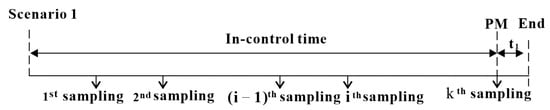
Figure 1.
The process of EWMA monitoring and maintenance in Scenario 1.
The expected IC and OOC time in can be obtained as
and the expected total time is
- Scenario 2:
Figure 2 shows that the production process starts in the IC state and shifts to the OOC state at time between interval when an assignable cause occurs, and the process parameter changes from to with The chart can detect the shift before the end of the th sampling, that is, the control chart first gives alarm at the th sampling, . When the process shift is detected, CM is adopted to restore the machine to an as-good-as-new state. The occurrence probability of scenario 2 () is given as follows:
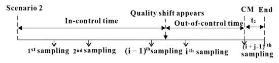
Figure 2.
The process of EWMA monitoring and maintenance in scenario 2.
The expected IC and OOC time in are
and
and the expected total time is
where is the average time from the last sampling to the occurrence of the shift, and according to the assumption that the time to the occurrence of an assignable cause follows the exponential distribution with parameter , therefore, is derived as follows:
- Scenario 3:
Figure 3 shows that the production process starts in an IC state and shifts to an OOC state at time between interval when an assignable cause occurs, and the process parameter changes from to with . However, due to the limits of the control chart’s capability, the monitoring scheme is unable to detect the quality shift until the end of the th sampling inspection and the inventory level reaches the maximum value . The process continues with no signal alert until the PM is scheduled. But, after checking and finding the true quality shift, a CM is carried out to replace the PM for repairing the machine to an as-good-as-new state. In this case, the occurrence probability of scenario 3 () can be given as
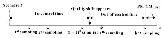
Figure 3.
The process of EWMA monitoring and maintenance in scenario 3.
The expected IC and OOC time in are easily obtained as
and
and the expected total time is
5. Production Cost and Production Cycle Time Analysis
The issue of production costs has long been the core concern for enterprises due to limited human, material, and financial resources, which motivates many researchers to establish an economic integration design of the production, maintenance, and quality control policy. Therefore, the production cost and production cycle time will be analyzed in this section for constructing the integrated model.
The expected production cost of one production cycle contains the expected quality loss cost, the expected sampling cost, the expected maintenance cost, the expected false alarm cost, the expected setup cost, and the expected cost of inventory control. As the production run time and the probability of each scenario are given in Section 4, the expected production cost and expected production cycle time for one production cycle will be introduced through the following expressions.
- (1)
- Expected quality loss cost
The defective items (or the non-conforming products) continues even when the process is monitored by the control chart. However, when the process is in the IC state, the proportion of the defective products is very low. When a process shift occurs, the key characteristic parameters of the products may deviate from the designed value, resulting in defective products being produced. There is an obvious fact that the quality loss cost of the OOC process is higher than that of the IC process. The quality loss cost can be expressed as
and
where and are the quality loss per time unit in the IC state and OOC state, and and can be estimated by the Taguchi quality loss function (Pan et al. [19]).
- (2)
- Expected sampling cost
Sampling cost happens when the control chart plots based on the sampling data to see whether the production process is in the IC state. To compute the sampling cost in each scenario, the average number of samplings needs to be found. From Figure 1, Figure 2 and Figure 3, we obtained that the numbers of samplings in scenario 1 and scenario 3 are . However, the number of samplings for scenario 2 is equal to , where a true signal is detected before the th sampling. Thus, the average cost of sampling is given by
and
where is the summation of the fixed and variable cost of each sampling.
- (3)
- Expected maintenance cost
The maintenance cost is different in three scenarios. As shown in Figure 3, the process is always in an IC state until the production stops and the PM cost will be included in scenario 1. However, in scenario 2, the process shift occurs and the control chart gives an alarm signal, therefore, the cost of CM should be considered. The maintenance cost of scenario 3 will be higher than the maintenance cost of scenario 2 because the process experiences both PM and CM actions. Therefore, the maintenance cost can be obtained as follows:
where
and represents the cost of maintenance in scenario .
- (4)
- Expected false alarm cost
A false alarm happens when the EWMA monitoring statistic exceeds the surveillance limits but the process is in the IC state. The false alarm exists because the control chart is constructed based on the theory of hypothesis testing, therefore, the cost of the false alarm should be taken into account, and it can be expressed as follows:
where
and represents the cost of inspecting a false alarm, and is the false alarm rate.
- (5)
- Expected setup cost
The expected setup cost in one production cycle can be given as
where
is the setup cost per production cycle.
- (6)
- Expected inventory control cost
A machine produces items at a rate of P. The products will be 100% inspected and defective products are discarded. We assume that the proportion of average defective items of the OOC process is a constant , where can be estimated from historical data (Bahria et al. [35]). However, for the IC process it is reasonably assumed that a very low proportion of defective products are produced, and we can ignore defective products. The expected average inventory control cost will be calculated for all possible conditions in one production cycle. Depending on whether the maintenance duration is less or longer than the inventory depletion period, two cases consisting of shortage and without shortage in one production process are considered, and each case under different production scenarios will be given as follows.
- (a)
- Scenario 1
- ■
- Case: without shortage:
Figure 4a shows the evolution of the average inventory level for the case without shortage in scenario 1. The expected inventory level contains two parts, and , which are respectively the average inventory holding level during the production uptime and production downtime. The duration of PM is smaller than , where represents the time from the inventory level to zero. Therefore, we have the following calculations:
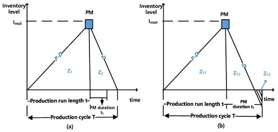
Figure 4.
Evolution of the inventory level in scenario 1: (a) case: without shortage; (b) case: with shortage.
The average inventory level in case (a) for scenario 1 is given by .
- ■
- Case: with shortage
Figure 4b shows the evolution of the expected inventory level for the case of shortage in scenario 1. In this scenario, the PM period is larger than the inventory consumption period, which can be expressed by
Let be the average inventory level. contains the inventory holding level and . Three functions, , , and , are given as
Therefore, the average inventory level in case (b) of scenario 1 is , and denotes the average shortage level.
- (b)
- Scenario 2
- ■
- Case: without shortage:
From Figure 5a, we can see that the duration of CM is less than or equal to the duration of the inventory consumption, and it can be expressed by
where and can be found in Equations (7) and (8). Let and respectively be the average inventory level during the production uptime and production downtime. and are described as
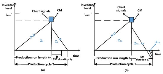
Figure 5.
Evolution of the inventory level in scenario 2: (a) case: without shortage; (b) case: with shortage.
The average inventory level is for the case of without shortage in scenario 2.
- ■
- Case: with shortage
For the case of shortage in scenario 2, the production process is disrupted by CM, and the period of CM is longer than the period of inventory consumption (see Figure 5b).
The average inventory level and the average shortage level are respectively expressed by
Finally, the average inventory level in case (b) for scenario 2 is , and is the average shortage level.
- (c)
- Scenario 3
- ■
- Case: without shortage:
As we can see from Figure 6a, the expected inventory level in one production cycle can be divided into two parts, and , and the maintenance duration is less than or equal to . The denotes the inventory consumption period starting from the time that the inventory is built up to the maximum value to the end of the production cycle.
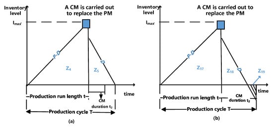
Figure 6.
Evolution of the inventory level in scenario 3: (a) case: without shortage; (b) case: with shortage.
and are respectively obtained as
Therefore, the average inventory level in case (a) for scenario 3 is .
- ■
- Case: with shortage
From Figure 6b, we can find that the period of maintenance is longer than the period of inventory consumption, where the relationship between and the period of the consumption of the inventory can be defined as
The equation for the average inventory level and shortage level is obtained using the following formula,
Therefore, the average inventory level in case (b) of scenario 3 is , and is the average shortage level.
Following the above analysis of the average inventory level, we define as the average inventory control cost, where contains the average inventory holding cost and the average shortage cost. For easy expression, we give three indicators in three scenarios as follows:
Finally, we define as follows:
- (7)
- Expected production cycle time
In different scenarios, we can find that the expected production cycle time depends on the production uptime, the maintenance duration, and the period of the inventory consumption. Therefore, the expected production cycle time can be given as
where is the average length of one production cycle in the occurrence of scenario , and can be expressed as follows:
6. Integrated Model of Production, EWMA Control, and Maintenance Policy
In this section, the integrated model of the production, EWMA control, and maintenance policy will be established based on the expected total cost per time unit (ETC), namely, the ETC model. Based on the ETC model, the objective is to minimize the ETC to achieve an optimal production level under the given constraints of the inventory size, the false alarm rate, the ARL of the OOC process, the sampling interval, the sample size, and sampling number. Further, the solution method will be introduced to deal with this optimization problem.
- (1)
- The objective function and constraints
The expected total cost per production cycle consists of expected quality loss cost , expected sampling inspection cost , expected maintenance cost and expected false alarm cost , expected cost of setup cost , and expected inventory control cost , and can be expressed by
The average expected total cost of one production cycle per time unit (ETC) is
To make the integrated model close to the real production process, sampling number , sampling interval , sample size , smooth parameter, inventory size , and type I error (Salmasnia et al. [16]; Zhou et al. [47]; Wan et al. [48]) and ARL of OOC processes are limited. Especially, the maximum value of the false alarm (Salmasnia et al. [16]) and the maximum ARL of the OOC process (Pan et al. [22], Salmasnia et al. [15]) should be prefixed. The optimization problem of the integrated model is formulated as follows:
subject to
where .
- (2)
- Solution approach
- The complexity of the presented integrated model leads to the difficulty of solving the objective function, where both the non-linear target and non-linear constraint functions increase the complexity of the model. In the literature, many efficient algorithms were developed to solve the optimization problem when establishing an integrated design of production, maintenance, and quality control policy, for example, Pan et al. [22] used Pattern Search Tool in MATLAB 7.0. Charongrattanasakul and Pongpullponsak [11], Yin et al. [30], and Huang et al. [14] adopted the genetic algorithm (GA). Salmasnia et al. [15] and Salmasnia et al. [16] applied meta-heuristic algorithms, etc. Without loss of generality, the GA is adopted to solve the optimization problem defined in Equations (46)–(54). The solution steps using the GA are shown in Table 2:
Table 2. Genetic Algorithm for Optimal ETC.
7. Case Study and Analysis
In Section 6, an integrated model for production, EWMA control, and maintenance policy is established, and the GA solution method is also provided. To show the application of the proposed model, first, a real example of a vibroseis equipment production process is introduced. Then, a comparative study is conducted between the integrated model established using the control chart and the proposed model. Finally, the sensitivity analysis is performed to investigate the influence of key input parameters on the objective function and decision parameters.
- (1)
- Case study
In this subsection, a real example of a vibroseis equipment production process is adopted to illustrate the application of the proposed model, where the vibroseis equipment’s bolt is one of the widespread parts used in vibroseis equipment. Vibrators installed on trucks of a vibroseis continuously impact the ground to generate seismic waves. The bolts play a crucial role in fixing various structures. Therefore, the quality and lifespan of vibroseis bolts are of great importance. The hardness is one of the key quality characteristics of the vibroseis equipment’s bolt and is mainly influenced by the heating temperature. Due to some assignable causes, the heating temperature will deviate from the target value, resulting in the hardness being unqualified and further leading to an increase in the proportion of defective bolts. Therefore, the EWMA control chart is adopted to monitor the heating temperature of the high-voltage rotor bolt production process.
To provide an optimal design of production, maintenance, and quality control policy for this bolt production process and minimize the production cost, the proposed integrated model is applied. According to the historical data and the information collected from engineers of the vibroseis equipment’s bolt production process, some input parameters are given in Table 3.
Table 3.
Input parameters for the vibroseis equipment’s bolt production process.
From Table 3, we can see that the production process stays in an IC state for an average of 100 h because of the shift parameter . Moreover, the average magnitude of the shift when the process goes OOC is approximately 0.25 standard variance. With variables detailed and constraints specified, the ETC and decision variables can be obtained by solving Expression (47) subject to
Figure 7 shows the iteration process of the GA for calculating the optimal ETC with 0.25. It can be seen that the values of the ETC under iterations 146–196 are approximately the same, which means that the ETC has not been remarkably improved during iterations 146–196. Therefore, it can be concluded with high confidence that the obtained results are very close to the real optimal solution. Finally, the optimal solution of decision parameters is , and the ETC is 242.6404. It is suggested by these results that, during one production cycle, 75 sampling instances are needed, and one should take one sample of size 20 every 4 h. The coefficient of the control limits of the EWMA control chart should be set at 1.6429 and the smooth parameter is recommended to be 0.3952. Moreover, the economic production quantity (EPQ) for one production cycle is , and the maximum inventory level is , which means that the utilization rate of inventory capacity is 100%.
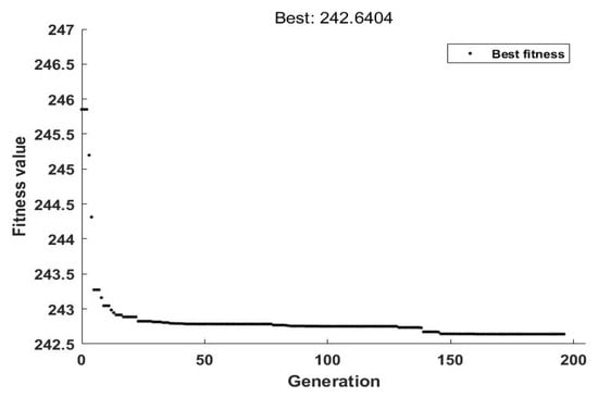
Figure 7.
The iteration process of the GA for the case of 0.25.
- (2)
- Comparison
Since there is no existing design for performing preventive maintenance (PM) based on information from the EWMA control chart and inventory level, a comparative study is conducted among three models: the model without monitoring, the model using the chart, and the proposed method. The comparison results are presented in Table 4. In the model using the chart, the assumptions, maintenance policies, and inventory control strategy are consistent with those of the proposed model using the EWMA chart. However, the decision parameters for the control chart model include the sampling number sampling number , sampling interval , sample size , and coefficient of the control limits of control chart. As shown in Table 4, the proposed model is the most economical. Furthermore, the proposed model is superior to the model without monitoring.
Table 4.
The comparison results of the proposed model, the model without monitoring, and the model based on the chart.
It can also be concluded that the economic performance of the proposed integrated method based on the EWMA control chart is superior to the traditional integrated model based on the control chart, because the ETC of our model is consistently less than the model of using the control chart. For example, the ETC of our proposed model based on the EWMA control chart is 242.6404 when shift is 0.25, while the ETC of the model based on the control chart is 250.7435.
- (3)
- Sensitivity analysis
In this subsection, the effect of parameters on the ETC is investigated. To quickly capture the relationship between the input parameters and the ETC under the same shift , the experiment design is first considered. Second, the effects of on the ETC and decision parameters are also given.
The orthogonal experimental design (ODE) method is a well-known experimental design method, where both the characteristics of the uniformly dispersed and symmetrical comparability exist, and the ODE can significantly reduce the number of experiments when there are many influence factors and levels. Salmasnia et al. [13] once adopted a Taguchi ODE to analyze the effect of input parameters on two comparative models. Motivated by Salmasnia et al. [13] and Wan [45], a numerical experiment using the ODE is also taken in this subsection.
For exploring the effect of eleven parameters on the ETC adequately, the number of parameter levels is set to 3. Detailed arrangements of experiments by ODE under the case of are listed in Table 5, and corresponding results of decision parameters and the ETC are recorded. Especially, to better understand the influence of eleven input parameters on the ETC, the results of the range analysis are also summarized in the last line of Table 5. The values of I, II, and III are prepared for calculating the range value R, and W represents the summarization of I, II, and III under the same parameter. The range value R is expressed as under the same parameter. We define that is the summation of ETC under the same parameter level and I, II, and III are respectively the mean of . For example, the first value 149.38 for row 29 in Table 4 is the mean of under 0.001 and = 50.64.
Table 5.
The Orthogonal experimental design for sensitivity analysis when .
For clear observation, the analysis of the effect of input parameters on the ETC is reported in Figure 8. Furthermore, the effects of on the ETC and decision parameters are plotted in Figure 9. The results of sensitivity analysis can be concluded as follows.
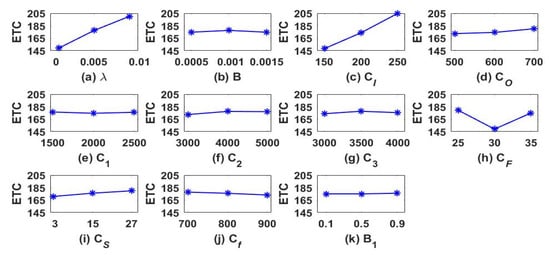
Figure 8.
The graphical representation of the main effects of eleven input parameters on the ETC.
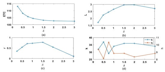
Figure 9.
The sensitivity analysis: (a) The effect of on ETC; (b) The effect of on ; (c) The effect of on r; (d) The effect of .
- ■
- Effect of eleven key parameters on the ETC
From Figure 8, the following conclusions are obtained.
- (1)
- (2)
- Eight parameters have a smaller effect on the ETC.
- (3)
- Moreover, one can find that the increase in the parameters , , , and can lead to an increase in the ETC. This phenomenon is consistent with the common knowledge that the occurrence rate of shift increases will increase the production cost per unit time. It is also obvious that increasing the quality loss cost parameter in the IC process, the quality loss cost parameter in the OOC process, and the varied sampling cost parameter will also increase the ETC.
- (4)
- It is worth pointing out that the increase in can reduce the ETC because the decision parameters can be adjusted to compensate the impact of the increase in the on ETC.
- ■
- Effect of δ on decision parameters and the ETC
From Figure 9, we can obtain the following conclusions.
- (1)
- When the magnitude of shift increases, the ETC decreases.
- (2)
- Figure 9b shows that, as increases, the coefficient of the control limits of the EWMA control chart increases under moderate and small shifts .
- (3)
- One can also conclude from Figure 9c that, as increases, the value of the smooth parameter increases under moderate and small shifts . However, the value of the smooth parameter shows a downward trend when .
There exists strong interaction between parameters and (see Figure 9d). The decision parameter increases (decreases), the parameter decreases (increases). It is because the process needs to satisfy the constraint that two decision parameters are adjusted to realize the minimized ETC.
8. Conclusions
In this paper, considering production quality and inventory constraints, we developed an integrated model of the production, EWMA control, and maintenance policy. The EWMA charting scheme is adopted to guarantee the process quality, efficiently detect moderate and small shifts, and reduce the quality loss cost. Considering the inventory size of the production process is finite in practice, a limited inventory size is considered in the proposed model. From the viewpoint of taking the opportunity to improve the state of the system, the PM action is carried out both considering the IC information given by the EWMA control chart and the inventory state. Finally, the proposed integrated model is applied to a vibroseis equipment’s bolt production process, and the decision parameters are given for arranging high-quality production. The corresponding results show that the production costs for the bolt production process are greatly reduced, which demonstrates the proposed model is more economic. Therefore, the proposed model is more suitable to be recommended to production decision-makers.
Despite the above contributions, this study has several limitations that suggest valuable directions for future research. First, the model relies on the assumption of perfect detection, where faults are always identified once they occur. In practice, detection systems may exhibit varying reliability, and incorporating imperfect detection processes represents an important extension. Second, parameters such as the failure rate are treated as fixed, while in real settings they may change over time or be influenced by external factors; developing more dynamic models would enhance practical applicability. Furthermore, the current work assumes that the occurrence of an assignable cause does not affect the process variance, and the quality characteristic follows a normal distribution. Future studies could investigate joint monitoring schemes for both mean and variance under non-normal distributions. Moreover, this study focuses on a single quality characteristic and a single-machine system. Research could be extended to incorporate multiple quality characteristics and multimachine manufacturing environments, which pose greater complexity but are more representative of actual industrial systems. Finally, relaxing other simplifying assumptions, such as immediate maintenance resource availability, would further improve the model’s robustness and broaden its applicability.
Supplementary Materials
The following supporting information can be downloaded at: https://www.mdpi.com/article/10.3390/axioms14090703/s1, Markov chain method for calculating run-length (RL) of the EWMA chart.
Author Contributions
Methodology, N.X.; Software, Z.L.; Writing—original draft, Y.Z. and N.X.; Writing—review and editing, N.X. and J.F. All authors have read and agreed to the published version of the manuscript.
Funding
This work was supported by Special project for cultivating scientific and technological innovation teams of Shandong Earthquake Agency (TD202303), Key tasks and special projects of Shandong Earthquake Agency (YW2305).
Data Availability Statement
Data are contained within the article.
Conflicts of Interest
The authors declare no conflicts of interest.
References
- Zhang, Y.Z.; Cai, H.; Zhang, J.J. Weighted-Likelihood-Ratio-Based EWMA Schemes for Monitoring Geometric Distributions. J. Axioms 2024, 13, 392. [Google Scholar] [CrossRef]
- Alhidairah, S.; Alam, F.M.A.; Nassar, M. Failure Cause Analysis Under Progressive Type-II Censoring Using Generalized Linear Exponential Competing Risks Model with Medical and Industrial Applications. Axioms 2025, 14, 595. [Google Scholar] [CrossRef]
- Jafari, N.; Lopes, A.M. Fault Detection and Identification with Kernel Principal Component Analysis and Long Short-Term Memory Artificial Neural Network Combined Method. Axioms 2023, 12, 583. [Google Scholar] [CrossRef]
- Farahani, A.; Tohidi, H. Integrated optimization of quality and maintenance: A literature review. Comput. Ind. Eng. 2021, 151, 106924. [Google Scholar] [CrossRef]
- Hafidi, N.; EI Barkany, A.; EI Mhamedi, A. Joint optimization of production, maintenance, and quality: A review and research trends. Int. J. Ind. Eng. Manag. 2023, 14, 282–296. [Google Scholar] [CrossRef]
- Salameh, M.K.; Ghattas, R.E. Optimal just-in-time inventory for regular preventive maintenance. J. Prod. Econ. 2001, 74, 157–161. [Google Scholar] [CrossRef]
- Goel, H.D.; Grievink, J.; Weijnen, M.P.C. Integrated optimal reliable design, production, and maintenance planning for multipurpose process plants. Comput. Chem. Eng. 2003, 27, 1543–1555. [Google Scholar] [CrossRef]
- El-Ferik, S. Economic production lot-sizing for an unreliable machine under imperfect age-based maintenance policy. Eur. J. Oper. Res. 2008, 186, 150–163. [Google Scholar] [CrossRef]
- Nahas, N. Buffer allocation and preventive maintenance optimization in unreliable production lines. J. Intell. Manuf. 2017, 28, 85–93. [Google Scholar] [CrossRef]
- Ben-Daya, M.; Rahim, M. Effect of maintenance on the economic design of x control chart. Eur. J. Oper. Res. 2000, 120, 131–143. [Google Scholar] [CrossRef]
- Charongrattanasakul, P.; Pongpullponsak, A. Minimizing the cost of integrated systems approach to process control and maintenance model by EWMA control chart using genetic algorithm. Expert Syst. Appl. 2011, 38, 5178–5186. [Google Scholar] [CrossRef]
- Xiang, Y. Joint optimization of X-control chart and preventive maintenance policies: A discrete-time Markov chain approach. Eur. J. Oper. Res. 2013, 229, 382–390. [Google Scholar] [CrossRef]
- Duan, C.Q.; Deng, C.; Gharaei, A.; Wu, J.; Wang, B.R. Selective maintenance scheduling under stochastic maintenance quality with multiple maintenance actions. Int. J. Prod. Res. 2018, 56, 7160–7178. [Google Scholar] [CrossRef]
- Huang, S.; Yang, J.; Xie, M. A double-sampling SPM scheme for simultaneously monitoring of location and scale shifts and its joint design with maintenance strategies. J. Manuf. Syst. 2020, 54, 94–102. [Google Scholar] [CrossRef]
- Salmasnia, A.; Abdzadeh, B.; Namdar, M. A joint design of production run length, maintenance policy and control chart with multiple assignable causes. J. Manuf. Syst. 2017, 42, 44–56. [Google Scholar] [CrossRef]
- Salmasnia, A.; Kaveie, M.; Namdar, M. An integrated production and maintenance planning model under VP-T2 Hotelling chart. Comput. Ind. Eng. 2018, 118, 89–103. [Google Scholar] [CrossRef]
- Hadian, S.M.; Farughi, H.; Rasay, H. Joint planning of maintenance, buffer stock and quality control for unreliable imperfect manufacturing systems. Comput. Ind. Eng. 2021, 157, 107304. [Google Scholar] [CrossRef]
- Zhang, N.; Tian, S.; Xu, J.T.; Deng, Y.J.; Cai, K.Q. Optimal production lot-sizing and condition-based maintenance policy considering imperfect manufacturing process and inspection errors. Comput. Ind. Eng. 2023, 177, 108929. [Google Scholar] [CrossRef]
- Ben-Daya, M.; Makhdoum, M. Integrated production and quality model under various preventive maintenance policies. J. Oper. Res. Soc. 1998, 49, 840–853. [Google Scholar] [CrossRef]
- Rahim, M.A.; Ben-Daya, M. A generalized economic model for joint determination of production run: Inspection schedule and control chart design. Int. J. Prod. Res. 1998, 36, 277–289. [Google Scholar] [CrossRef]
- Pandey, D.; Kulkarni, M.S.; Vrat, P. A methodology for joint optimization for maintenance planning, process quality and production scheduling. Comput. Ind. Eng. 2011, 61, 1098–1106. [Google Scholar] [CrossRef]
- Pan, E.; Jin, Y.; Wang, S.H.; Cang, T. An integrated EPQ model based on a control chart for an imperfect production process. Int. J. Prod. Res. 2012, 50, 6999–7011. [Google Scholar] [CrossRef]
- Bahria, N.; Chelbi, A.; Dridi, I.H.; Bouchriha, H. Maintenance and quality control integrated strategy for manufacturing systems. Eur. J. Ind. Eng. 2018, 12, 307–331. [Google Scholar] [CrossRef]
- Salmasnia, A.; Hajihosseini, Z.; Namdar, M.; Mamashli, F. A joint determination of production cycle length, maintenance policy, and control chart parameters considering time value of money under stochastic shift size. Sci. Iran. 2020, 27, 427–447. [Google Scholar] [CrossRef]
- Shi, L.X.; Lv, X.L.; He, Y.D.; He, Z. Optimising production, maintenance, and quality control for imperfect manufacturing systems considering timely replenishment. Int. J. Prod. Res. 2024, 62, 3504–3525. [Google Scholar] [CrossRef]
- Serel, D.A.; Moskowitz, H. Joint economic design of EWMA control charts for mean and variance. Eur. J. Oper. Res. 2008, 184, 157–168. [Google Scholar] [CrossRef]
- Ardakan, M.A.; Hamadani, A.Z.; Sima, M.; Reihaneh, M. A hybrid model for economic design of MEWMA control chart under maintenance policies. Int. J. Adv. Manuf. Technol. 2016, 83, 2101–2110. [Google Scholar] [CrossRef]
- Hesamian, G.; Akbari, M.G.; Ranjbar, E. Exponentially weighted moving average control chart based on normal fuzzy random variables. Int. J. Fuzzy Syst. 2019, 21, 1187–1195. [Google Scholar] [CrossRef]
- Sukparungsee, S.; Areepong, Y.; Taboran, R. Exponentially weighted moving average-moving average charts for monitoring the process mean. PLoS ONE 2020, 15, e0228208. [Google Scholar]
- Yin, H.; Zhu, H.; Zhang, G.; Deng, Y. Design of MEWMA control chart for process subject to quality shift and equipment failure. In Proceedings of the 2015 9th International Conference on Application of Information and Communication Technologies (ICAICT), Rostov on Don, Russia, 14–16 October 2015; pp. 404–407. [Google Scholar]
- Noman, M.A.; Al-Shayea, A.; Nasr, E.A.; Kaid, H.; Mahmoud, H.A. A model for maintenance planning and process quality control optimization based on EWMA and CUSUM control charts. Trans. Famena 2021, 45, 95–116. [Google Scholar] [CrossRef]
- Nourelfath, M.; Nahas, N.; Ben-Daya, M. Integrated preventive maintenance and production decisions for imperfect processes. Reliab. Eng. Syst. Saf. 2016, 148, 21–31. [Google Scholar] [CrossRef]
- Bouslah, B.; Gharbi, A.; Pellerin, R. Integrated production, sampling quality control and maintenance of deteriorating production systems with AOQL constraint. Omega 2016, 61, 110–126. [Google Scholar] [CrossRef]
- Rivera-Gómez, H.; Gharbi, A.; Kenné, J.P.; Montaño-Arango, O.; Corona-Armenta, J.R. Joint optimization of production and maintenance strategies considering a dynamic sampling strategy for a deteriorating system. Comput. Ind. Eng. 2020, 140, 106273. [Google Scholar] [CrossRef]
- Bahria, N.; Chelbi, A.; Bouchriha, H.; Dridi, I.H. Integrated production, statistical process control, and maintenance policy for unreliable manufacturing systems. Int. J. Prod. Res. 2019, 57, 2548–2570. [Google Scholar] [CrossRef]
- He, Y.; Liu, F.; Cui, J.; Han, X.; Zhao, Y.; Chen, Z.; Zhang, A. Reliability-oriented design of integrated model of preventive maintenance and quality control policy with time-between-events control chart. Comput. Ind. Eng. 2019, 129, 228–238. [Google Scholar] [CrossRef]
- Fakher, H.B.; Mourelfath, M.; Gendreau, M. A cost minimisation model for joint production and maintenance planning under quality constraints. Int. J. Prod. Res. 2017, 55, 2163–2176. [Google Scholar] [CrossRef]
- Mokhtari, H.; Asadkhani, J. Extended economic production quantity models with preventive maintenance. Sci. Iran. 2020, 27, 3253–3264. [Google Scholar]
- Lin, Y.H.; Chen, Y.C.; Wang, W.Y. Optimal Production Model for Imperfect Process with Imperfect Maintenance, Minimal Repair and Rework. Int. J. Syst. Sci. Oper. Logist. 2016, 4, 229–240. [Google Scholar] [CrossRef]
- Duffuaa, S.; Kolus, A.; AI-Turki, U.; EI-Khalifa, A. An Integrated Model of Production Scheduling, Maintenance and Quality for a Single Machine. Comput. Ind. Eng. 2020, 142, 106239. [Google Scholar] [CrossRef]
- Wan, Q.; Zhu, M.; Qiao, H. A joint design of production, maintenance planning and quality control for continuous flow processes with multiple assignable causes. CIRP J. Manuf. Sci. Technol. 2023, 43, 214–226. [Google Scholar] [CrossRef]
- Lv, X.; Shi, L.; He, Y.; He, Z. Joint optimization of production, inspection, and maintenance under finite time for smart manufacturing systems. Reliab. Eng. Syst. Saf. 2025, 253, 110490. [Google Scholar] [CrossRef]
- Gaver, D.P. Operating Characteristics of a Simple Production, Inventory-Control Model. Oper. Res. 1961, 9, 635–649. [Google Scholar] [CrossRef]
- Sobel, M.J. Optimal Average-cost Policy for a Queue with Start-up and Shut-down Costs. Oper. Res. 1969, 17, 145–162. [Google Scholar] [CrossRef]
- Lin, H.J. An Economic Production Quantity Model with Backlogging and Imperfect Rework Process for Uncertain Demand. Int. J. Prod. Res. 2019, 59, 467–482. [Google Scholar] [CrossRef]
- Seif, A. A New Markov Chain Approach for the Economic Statistical Design of the VSS T2 Control Chart. Commun. Stat.-Simul. Comput. 2019, 48, 200–218. [Google Scholar] [CrossRef]
- Zhou, P.; Wei, H.; Zhang, H. Selective Reviews of Bandit Problems in AI via a Statistical View. Mathematics 2025, 13, 665. [Google Scholar] [CrossRef]
- Wan, Q. Economic-statistical Design of Integrated Model of VSI Control Chart and Maintenance Incorporating Multiple Dependent State Sampling. IEEE Access 2020, 8, 87609–87620. [Google Scholar] [CrossRef]
Disclaimer/Publisher’s Note: The statements, opinions and data contained in all publications are solely those of the individual author(s) and contributor(s) and not of MDPI and/or the editor(s). MDPI and/or the editor(s) disclaim responsibility for any injury to people or property resulting from any ideas, methods, instructions or products referred to in the content. |
© 2025 by the authors. Licensee MDPI, Basel, Switzerland. This article is an open access article distributed under the terms and conditions of the Creative Commons Attribution (CC BY) license (https://creativecommons.org/licenses/by/4.0/).