Multiple Solutions of Fractional Kazdan–Warner Equation for Negative Case on Finite Graphs

Abstract

This work establishes the multiplicity of solutions for the fractional Kazdan–Warner equation on finite graphs for the negative case. Our main focus lies in analyzing the nonlinear equation defined on a finite graph $(V,E,\mu ,w)$: ${(-\Delta )}^{s}u=(K+\lambda )e^{2u}-\kappa \mathrm{in}V,$ where the fraction $s\in (0,1)$ and real parameter $\lambda$ are given, and the graph functions K and $\kappa$ satisfy ${\max }_{x\in V}K\left(x\right)=0$, $K\not\equiv 0$ and ${\int }_V\kappa d\mu <0$. We derive the solvability characteristics of the above equation with the help of variational theory and the upper and lower solutions method.

1. Introduction

The Kazdan–Warner equation emerges from a fundamental geometric problem concerning the prescription of Gaussian curvature on a Riemann surface. Let $(\Sigma ,g)$ be a two-dimensional closed Riemannian manifold and $\tilde{g}=e^{2\phi }g$ denote a conformal metric to g defined by some function $\phi \in C^{\infty }(\Sigma )$. The curvature prescription problem requires solving the nonlinear elliptic equation:

$${\Delta }_g\phi =K{e}^{2\phi }-\kappa ,$$

(1)

where ${\Delta }_g$ represents the Laplacian on $(\Sigma ,g)$, $\kappa$ and K denote the Gaussian curvature associated with g and $\tilde{g}$, respectively. Through the substitution $\psi :=\phi -u/2$, where u satisfies ${\Delta }_{g}u=2\overline{\kappa }-2\kappa$ with $\overline{\kappa }:={\int }_{\Sigma }\kappa d{v}_g/|\Sigma |$, Equation (1) transforms into the normalized curvature equation:

$${\Delta }_{g}u=2K{e}^{2\psi }{e}^u-2\overline{\kappa }.$$

Therefore, under a conformal transformation, this reformulation demonstrates the equivalence between curvature prescription and solving the above equation. Abstracting from geometric constraints leads to the canonical form:

$${\Delta }_{g}u=h{e}^u-c,$$

(2)

where $h\in C^{\infty }(\Sigma )$ and $c\in \mathbb{R}$ become independent parameters. In the seminal and fundamental work of Kazdan–Warner [1,2], the solvability of (2) was described almost completely by them. Subsequent developments (see Chen-Li [3], Ding-Jost-Li-Wang [4], and related works) extended these results through refined analytic techniques and geometric interpretations.

The study of solution multiplicity for the Kazdan–Warner equation in negative curvature regimes constitutes a significant research direction. Consider the modified equation on $(\Sigma ,g)$:

$${\Delta }_{g}u=(K+\lambda )e^{2u}-\kappa ,$$

(3)

where $\overline{\kappa }<0$, $K\le 0$, $K\not\equiv 0$ and $\lambda \in \mathbb{R}$. Ding and Liu [5] established fundamental existence results through variational methods: there has a unique solution if $\lambda \le 0$; there is a threshold ${\lambda }^{\ast }>0$ such that the above equation has at least two distinct solutions when $0<\lambda <{\lambda }^{\ast }$, at least one solution when $\lambda ={\lambda }^{\ast }$, and no solution when $\lambda >{\lambda }^{\ast }$. Borer, Galimberti, and Struwe [6] later recovered portions of these results using Struwe’s monotonicity technique in [7], while Yang and Zhu [8] generalized them to conical metric spaces.

The discrete counterpart presents distinct challenges, as Gaussian curvature prescriptions on graphs lack direct geometric interpretations. Grigor’yan, Lin, and Yang [9] pioneered the finite graph adaptation of (2). Subsequent developments include Ge’s critical case analysis in [10]; p-Laplacian generalizations by Ge [11] and Zhang-Chang [12]; infinite graph extensions by Ge-Jiang [13]; compactifiable graph studies from Keller-Schwarz [14]; topological degree approaches via Sun-Wang [15].

For the multiplicity results of the Kazdan–Warner Equation (3) on finite graphs, S. Liu and Yang [16] established a discrete analog of [5] through the upper-lower solution method and variational calculus. Y. Liu and Yang [17] verified similar conclusions via topological degree theory. Additional investigations of nonlinear PDEs on graphs appear in [18,19,20,21,22,23,24], demonstrating the field’s continued expansion.

On the other hand, the mathematical investigation of fractional Laplace operators traces its origins to Riesz’s foundational work on singular integrals [25], where they appear in conservation laws [26], in minimal surfaces [27], in gravitational optics [28], in stratified materials [29], in quantum mechanics [30], in anomalous diffusion and probability [31], and so on. Seminal works [32,33,34,35,36] provide comprehensive treatments of the subject, detailing both theoretical foundations and applied perspectives. On Euclidean space ${\mathbb{R}}^N$, the fractional Laplacian admits ten equivalent characterizations [35], such as a Fourier multiplier, an operator associated with a Dirichlet form construction, a singular integral operator, the inverse of the Riesz potential operator, or a generator of a contractive heat semigroup.

This paper focuses on the definition given by the heat semigroup: for any fraction $s\in (0,1)$, the fractional Laplacian ${(-\Delta )}^s$ is defined by

$$\begin{array}{c}\hfill {(-\Delta )}^{s}u\left(x\right)={\displaystyle \frac{s}{\Gamma (1-s)}}{\int }_0^{+\infty }{\displaystyle \frac{1}{t^{1+s}}}\left(u\left(x\right)-e^{t\Delta }u\left(x\right)\right)dt,\end{array}$$

(4)

where $e^{t\Delta }$ is the heat semigroup of $\Delta$, and $\Gamma (·)$ denotes the Gamma function. For discrete cases, (4) on the integer lattice graph $\mathbb{Z}$ was studied in [37,38], and an equivalent form was given as

$$\begin{array}{c}\hfill {(-\Delta )}^{s}u\left(x\right)=\sum _{y\in V}{K}_s(x-y)\left(u\left(x\right)-u\left(y\right)\right)\end{array}$$

(5)

for any $u\in L^2\left(\mathbb{Z}\right),$ where the discrete kernel

$$\begin{array}{c}\hfill K_s\left(x\right)={\displaystyle \frac{s}{\Gamma (1-s)}}{\int }_0^{+\infty }{\displaystyle \frac{1}{t^{1+s}}}{e}^{t\Delta }{1}_0\left(x\right)dt\end{array}$$

and $1_y$ denotes the characteristic function of $y\in \mathbb{Z}$ with $1_0(x-y)=1_y\left(x\right)$. Moreover, (4) was studied in [39] on N-dimensional lattice graph ${\mathbb{Z}}^N$ ($N\ge 1$). When $G=(V,E,\mu ,w)$ is a stochastically complete graph with standard measure and weight, (4) was studied by [40], and an equivalent form was written as (5). The stochastically complete graph means that the weighted graph G satisfies

$$\begin{array}{c}\hfill \sum _{y\in V}{h}_t(x,y)\mu \left(y\right)=1\end{array}$$

for any $t>0$ and $x\in V,$ where $h_t(x,y)=e^{t\Delta }(1_y\left(x\right)/\mu \left(y\right))$ denotes the heat kernel on G. Notice that finite graphs are stochastically complete, and that $h_t(x,y)$ can be expressed in terms of eigenvalues and eigenfunctions of $-\Delta$ on any finite graph. Starting by this point, if V is finite, (4) was studied in [41], and an equivalent form was derived as

$$\begin{array}{c}\hfill {(-\Delta )}^{s}u\left(x\right)={\displaystyle \frac{1}{\mu \left(x\right)}}\sum _{y\in V,y\ne x}{H}_s(x,y)\left(u\left(x\right)-u\left(y\right)\right)\end{array}$$

(6)

for any $u\in C\left(V\right)$, where the symmetric positive function

$$\begin{array}{c}\hfill H_s(x,y)={\displaystyle \frac{s\mu \left(x\right)\mu \left(y\right)}{\Gamma (1-s)}}{\int }_0^{+\infty }{\displaystyle \frac{1}{t^{1+s}}}{h}_t(x,y)dt\end{array}$$

(7)

for any $x\ne y\in V$. Moreover, ref. [41] got an explicitly represented of ${(-\Delta )}^s$ as

$$\begin{array}{c}\hfill {(-\Delta )}^{s}u\left(x\right)=\sum _{i=1}^n{\lambda }_i^s{\varphi }_i\left(x\right)⟨u,{\varphi }_i⟩,\end{array}$$

where $n=♯V$ is the count of all distinct vertices in V, ${\lambda }_i$ and ${\varphi }_i$ ($i=1,\cdots ,n$) are the eigenvalues of $-\Delta$ and the corresponding orthogonal eigenfunctions, respectively. In addition, they also studied the solvability of (2) on finite graphs. A recent investigation by Zhang et al. [42] extended this framework to stochastically complete graphs with arbitrary vertex measures and edge weights. Other discrete counterparts of fractional Laplacian have been established through multiple approaches, mirroring their continuous analogs, as detailed in [43,44,45,46,47]. These works bridge nonlocal operators with graph theory, enabling systematic study of fractional elliptic equations on discrete networks.

In this paper, we aim to solve this problem of multiple solutions of the fractional Kazdan–Warner equation on graphs in the negative case, which extends the result of S. Liu-Yang [16] to the fractional case. Specifically, assuming that $G=(V,E,\mu ,w)$ is a connected finite graph, we focus on the fractional Kazdan–Warner equation:

$$\begin{array}{c}\hfill {(-\Delta )}^{s}u=K_{\lambda }{e}^{2u}-\kappa \mathrm{in}V,\end{array}$$

(8)

where the fraction $s\in (0,1)$, the fractional Laplacian ${(-\Delta )}^s$ is defined as in (6), the function $\kappa :V\to \mathbb{R}$ satisfies ${\int }_V\kappa d\mu <0$ and the function $K_{\lambda }:V\to \mathbb{R}$ is equal to $K+\lambda$. Here, $\lambda$ is a real number, and $K:V\to \mathbb{R}$ is a function satisfying ${\max }_{x\in V}K\left(x\right)=0$ and $K\not\equiv 0$. Now, let us present our main results.

Theorem 1.

For any $\lambda \le 0$, the fractional Kazdan–Warner Equation (8) has a unique solution.

Theorem 2.

There has a critical parameter ${\lambda }_s\in (0,-{\min }_{x\in V}K\left(x\right))$ such that (8) has at least two distinct solutions when $\lambda \in (0,{\lambda }_s)$, at least one solution when $\lambda ={\lambda }_s$, and no solution when $\lambda >{\lambda }_s$.

The rest of the paper is organized as follows. In Section 2, we review some concepts about graphs and give some important lemmas. In Section 3, we verify Theorem 1. In Section 4, we prove Theorem 2. In Section 5, we show some examples.

2. Preparation

We begin by formalizing the graph theoretic framework essential for our analysis. Let $(V,E)$ be a connected, simple, undirected graph with a finite set of vertices V and a finite set of edges E. Here, connectivity ensures pairwise vertex linkage through finite edges, simplicity prohibits loops, or multiple edges, and undirectedness implies symmetry in edge relations ($x\sim y\iff y\sim x$). Each vertex $x\in V$ carries a positive measure $\mu \left(x\right)>0$, while edges $[x,y]\in E$ possess symmetric weights $w_{xy}=w_{yx}>0$. Throughout this paper, $G=(V,E,\mu ,w)$ always means a finite, connected, simple, undirected, weighted graph.

We now introduce some concepts of integral and function spaces. Let $C\left(V\right)$ be the space of all real-valued functions on the graph G. The integral of a function $u\in C\left(V\right)$ is defined by ${\int }_{V}ud\mu ={\sum }_{x\in V}u\left(x\right)\mu \left(x\right).$ For $1\le q<+\infty$, the Lebesgue space $L^q\left(V\right)$ consists of functions $u\in C\left(V\right)$ with finite norm ${\parallel u\parallel }_{L^q\left(V\right)}={\left({\sum }_{x\in V}{\left|u\left(x\right)\right|}^q\mu \left(x\right)\right)}^{1/q},$ while $L^{\infty }\left(V\right)$ contains bounded functions under the norm ${\parallel u\parallel }_{L^{\infty }\left(V\right)}={\sup }_{x\in V}\left|u\left(x\right)\right|.$ Throughout this work, we adopt the concise notation ${\parallel ·\parallel }_q$ and ${\parallel ·\parallel }_{\infty }$ for these norms.

We next review some important definitions in [41]. The fractional Laplacian ${(-\Delta )}^s$ acting on a function $u\in C\left(V\right)$ is defined by (6). Assign the inner product of the fractional gradient as

$$\begin{array}{c}\hfill {\nabla }^s\phi {\nabla }^{s}u\left(x\right)={\displaystyle \frac{1}{2\mu \left(x\right)}}\sum _{y\in V,y\ne x}{H}_s(x,y)(\phi \left(x\right)-\phi \left(y\right))(u\left(x\right)-u\left(y\right))\end{array}$$

(9)

for any $\phi ,u\in C\left(V\right)$. Particularly, $|{\nabla }^{s}u|\left(x\right)=\sqrt{{\nabla }^{s}u{\nabla }^{s}u\left(x\right)}$. Moreover, it follows from [Proposition 3.6] [41] that

$$\begin{array}{c}\hfill {\int }_V\phi {(-\Delta )}^{s}ud\mu ={\int }_V{\nabla }^{s}u{\nabla }^s\phi d\mu ={\int }_{V}u{(-\Delta )}^s\phi d\mu \end{array}$$

(10)

for any u, $\phi \in C\left(V\right)$. Define the fractional Sobolev space $W^{s,2}\left(V\right)$ as

$$\begin{array}{c}\hfill W^{s,2}\left(V\right)=\left\{u\in C\left(V\right):{\int }_V\left(|{\nabla }^s{u|}^2+u^2\right)d\mu <+\infty \right\}\end{array}$$

for any $s\in (0,1)$, which is equipped with the associated norm

$$\begin{array}{c}\hfill {\parallel u\parallel }_{W^{s,2}\left(V\right)}={\left({\parallel u\parallel }_2^2+{\parallel {\nabla }^{s}u\parallel }_2^2\right)}^{{\displaystyle \frac{1}{2}}}.\end{array}$$

Since V is finite, then it is obvious that $W^{s,2}\left(V\right)$ is the set of all functions on G, then $W^{s,2}\left(V\right)$ is a finite-dimensional linear normed space, and is also a Banach space. Moreover, there are some important lemmas in [41].

Lemma 1

(Lemma 4.1 [41]). The fractional Sobolev space $W^{s,2}\left(V\right)$ is pre-compact, namely, if the function sequence ${\left\{u_i\right\}}_{i=1}^{\infty }$ is uniformly bounded in $W^{s,2}\left(V\right)$, then there is $u\in W^{s,2}\left(V\right)$ such that $u_i$ converges to u in $W^{s,2}\left(V\right)$ as $i\to +\infty$.

Lemma 2

(Lemma 4.4 [41]). For the perturbed fractional operator

$$\begin{array}{c}\hfill L_{s,\psi }\left(u\right):={(-\Delta )}^{s}u+\psi u,\end{array}$$

(11)

where $u\in C\left(V\right)$ and $\psi :V\to {\mathbb{R}}^{+}$ is strictly positive, the following hold:

(i) 

$L_{s,\psi }$ is bijective;

(ii) 

if $L_{s,\psi }\left(u\right)\le L_{s,\psi }\left(v\right)$, then $u\le v$.

Lemma 3

(Lemma 4.8 [41]). Given $\psi \in C\left(V\right)$, the equation

$$\begin{array}{c}\hfill {(-\Delta )}^{s}u=\overline{\psi }-\psi \end{array}$$

admits solutions unique up to additive constants, where $\overline{\psi }={\int }_V\psi d\mu /\left|V\right|$.

Moreover, we generalize [Lemma 4.5] [41] to the following:

Lemma 4.

A function $u^{+}\in C\left(V\right)$ is called an upper solution of (8) if

$$\begin{array}{c}\hfill {(-\Delta )}^s{u}^{+}\ge (K_{\lambda }{e}^{2u^{+}}-\kappa )onV,\end{array}$$

while $u^{-}\in C\left(V\right)$ is a lower solution if

$$\begin{array}{c}\hfill {(-\Delta )}^s{u}^{-}\le (K_{\lambda }{e}^{2u^{-}}-\kappa )onV.\end{array}$$

If there is an upper solution $u^{+}$ and a lower solution $u^{-}$ of (8) with $u^{+}\ge u^{-}$, then the fractional Kazdan–Warner Equation (8) has a solution $u^{\ast }$ that satisfies $u^{-}\le u^{\ast }\le u^{+}$.

Proof. 

Let $K_{\lambda }^{\ast }\left(x\right)=$$\max \{1,-2K_{\lambda }\left(x\right)\}$, then we obtain $K_{\lambda }^{\ast }\left(x\right)\ge 1$ and $K_{\lambda }^{\ast }\left(x\right)\ge -2K_{\lambda }\left(x\right)$. Let $L_{s,\psi }$ be defined by (11) with $\psi =K_{\lambda }^{\ast }{e}^{2u^{+}}>0$. We assign $u_0=u^{+}$ and inductively $u_{i+1}$ as

$$\begin{array}{c}\hfill L_{s,\psi }\left(u_{i+1}\right)=\psi u_i+K_{\lambda }{e}^{2u_i}-\kappa ,\forall i=0,1,2,\cdots .\end{array}$$

(12)

We claim that

$$\begin{array}{c}\hfill u^{-}\le u_{i+1}\le u_i\le \cdots \le u_1\le u^{+}.\end{array}$$

(13)

It is not difficult to see that

$$\begin{array}{c}\hfill L_{s,\psi }\left(u_1\right)-L_{s,\psi }\left(u^{+}\right)=-{(-\Delta )}^s{u}^{+}+K_{\lambda }{e}^{2u^{+}}-\kappa \le 0,\end{array}$$

and then $u_1\le u^{+}$ by Lemma 2. Suppose $u_i\le u_{i-1}\le u^{+}$, there is $\xi \in (u_i,u_{i-1})$ such that $e^{2u_{i-1}}-e^{2u_i}=2e^{2\xi }(u_{i-1}-u_i)$ from the mean value theorem. Therefore, one concludes that

$$\begin{array}{cc}\hfill L_{s,\psi }\left(u_{i+1}\right)-L_{s,\psi }\left(u_i\right)& =-\psi (u_{i-1}-u_i)-K_{\lambda }(e^{2u_{i-1}}-e^{2u_i})\hfill \\ \hfill & =-K_{\lambda }^{\ast }{e}^{2u^{+}}(u_{i-1}-u_i)-2K_{\lambda }{e}^{2\xi }(u_{i-1}-u_i)\hfill \\ \hfill & \le -K_{\lambda }^{\ast }(e^{2u^{+}}-e^{2\xi })(u_{i-1}-u_i)\hfill \\ \hfill & \le 0,\hfill \end{array}$$

which implies $u_{i+1}\le u_i$ by Lemma 2. Then by induction, we obtain

$$u_{i+1}\le u_i\le \cdots \le u_1\le u^{+}$$

for any i. Similarly, we also have by induction $u^{-}\le u_{i+1}$ for any i. Therefore, the claim in (13) holds.

Since V is finite and (13) holds, it is easy to see that there has a function $u^{\ast }$ satisfying $u^{-}\le u^{\ast }\le u^{+}$, such that $u_i\to u^{\ast }$ uniformly on V. Passing to the limit $i\to +\infty$ in (12), one concludes that $u^{\ast }$ is a solution of (8). □

3. Proof of Theorem 1

Denote an energy functional $J_{\lambda }\left(u\right):W^{s,2}\left(V\right)\to \mathbb{R}$ as

$$\begin{array}{c}\hfill J_{\lambda }\left(u\right)={\displaystyle \frac{1}{2}}{\int }_V{\left|{\nabla }^{s}u\right|}^{2}d\mu -{\displaystyle \frac{1}{2}}{\int }_V{K}_{\lambda }{e}^{2u}d\mu +{\int }_V\kappa ud\mu ,\end{array}$$

(14)

where $K_{\lambda }$ and $\kappa$ are given as in (8). In this section, we consider the solvability of (8) in the case of $\lambda \le 0$ and prove Theorem 1.

Lemma 5.

If $\lambda \le 0$, then $J_{\lambda }$ is strictly convex on $W^{s,2}\left(V\right)$, namely, there has a positive constant C such that

$$\begin{array}{c}\hfill d^2{J}_{\lambda }\left(u\right)\left(\psi \right)\ge C{\parallel \psi \parallel }_{W^{s,2}\left(V\right)}^2,\forall u,\psi \in W^{s,2}\left(V\right),\end{array}$$

(15)

where the 2-order Frechet derivative

$$\begin{array}{c}\hfill d^2{J}_{\lambda }\left(u\right)\left(\psi \right)={\int }_V\left(|{\nabla }^s{\psi |}^2-2{\psi }^2{K}_{\lambda }{e}^{2u}\right)d\mu .\end{array}$$

(16)

Proof. 

Assuming not, we can find $u\in W^{s,2}\left(V\right)$ and ${\left\{{\psi }_i\right\}}_{i=1}^{\infty }\subseteq W^{s,2}\left(V\right)$ such that ${∥{\psi }_i∥}_{W^{s,2}\left(V\right)}=1$ and $d^2{J}_{\lambda }\left(u\right)\left({\psi }_i\right)$ converges to 0 as $i\to +\infty ,$ and then

$$\begin{array}{c}\hfill {\int }_V{\left|{\nabla }^s{\psi }_i\right|}^{2}d\mu \to 0\mathrm{and}{\int }_V{K}_{\lambda }{e}^{2u}{\psi }_i^{2}d\mu \to 0.\end{array}$$

(17)

From Lemma 1, we obtain that there has ${\psi }_0\in W^{s,2}\left(V\right)$ such that

$$\begin{array}{c}\hfill \underset{i\to +\infty }{\lim }{∥{\psi }_i∥}_{W^{s,2}\left(V\right)}={∥{\psi }_0∥}_{W^{s,2}\left(V\right)}=1,\end{array}$$

(18)

which together with (17) leads to ${\psi }_0\equiv C_0$ and $C_0^2{\int }_V{K}_{\lambda }{e}^{2u}d\mu =0$, where $C_0$ is a constant. Since $K_{\lambda }=K+\lambda \le 0$ and $K\not\equiv 0$, we obtain ${\int }_V{K}_{\lambda }{e}^{2u}d\mu <0$, and then ${\psi }_0\equiv 0$. This contradicts (18), and then (15) follows. □

Proof of Theorem 1.

Obviously, $J_{\lambda }$ has a lower bound on $W^{s,2}\left(V\right)$ if $\lambda \le 0$, and then there is a real number $\theta :={\inf }_{u\in W^{s,2}\left(V\right)}{J}_{\lambda }\left(u\right)$. Take a function sequence ${\left\{u_i\right\}}_{i=1}^{+\infty }\subseteq W^{s,2}\left(V\right)$ such that $J_{\lambda }\left(u_i\right)\to \theta$ as $i\to +\infty$. We claim that $u_i$ is bounded in $W^{s,2}\left(V\right)$. For otherwise, $\parallel u_i{\parallel }_{W^{s,2}\left(V\right)}\to +\infty$, and then $\parallel u_i{\parallel }_2\to +\infty$ and $\parallel {\nabla }^s{u}_i{\parallel }_2\to +\infty$. Young’s inequality $ab\le ϵa^2+b^2/\left(4ϵ\right)$, $a,b\ge 0$, implies that

$$\left|{\int }_V\kappa u_{i}d\mu \right|\le {\int }_V\left|\kappa u_i\right|d\mu \le ϵ{\int }_V{u}_i^{2}d\mu +{\displaystyle \frac{1}{4ϵ}}{\int }_V{\kappa }^{2}d\mu .$$

Therefore, from $K_{\lambda }=K+\lambda \le 0$ and $K\not\equiv 0$, we obtain

$$\begin{array}{cc}\hfill J_{\lambda }\left(u_i\right)& ={\displaystyle \frac{1}{2}}{\int }_V{\left|{\nabla }^s{u}_i\right|}^{2}d\mu -{\displaystyle \frac{1}{2}}{\int }_V{K}_{\lambda }{e}^{2u_i}d\mu +{\int }_V\kappa u_{i}d\mu \hfill \\ \hfill & >{\displaystyle \frac{1}{2}}{\parallel {\nabla }^s{u}_i\parallel }_2^2+{\int }_V\kappa u_{i}d\mu \hfill \\ \hfill & \ge {\displaystyle \frac{1}{2}}\parallel {\nabla }^s{u}_i{\parallel }_2^2-ϵ{\parallel u_i\parallel }_2^2-{\displaystyle \frac{1}{4ϵ}}{\int }_V{\kappa }^{2}d\mu ,\hfill \end{array}$$

which contradicts $J_{\lambda }\left(u_i\right)\to \theta$. Hence, $u_i$ is bounded in $W^{s,2}\left(V\right)$. Therefore, it follows from Lemma 1 that there is $u_0\in W^{s,2}\left(V\right)$ such that $u_i$ converges to $u_0$ in $W^{s,2}\left(V\right)$, and then $J_{\lambda }\left(u_i\right)$ converges to $J_{\lambda }\left(u_0\right)$ as $i\to +\infty$. This implies $J_{\lambda }\left(u_0\right)=\theta$, and then $u_0$ is a critical point of $J_{\lambda }$.

We claim that $u_0$ is the unique critical point. Suppose not, let $u^{\ast }$ be another critical point of $J_{\lambda }$. Then $d{J}_{\lambda }\left(u_0\right)\left(\psi \right)=d{J}_{\lambda }\left(u^{\ast }\right)\left(\psi \right)=0$, where $d{J}_{\lambda }$ is the Frechet derivative of $J_{\lambda }$ and

$$\begin{array}{c}\hfill d{J}_{\lambda }\left(u\right)\left(\psi \right)={\int }_V\left({(-\Delta )}^{s}u-K_{\lambda }{e}^{2u}+\kappa \right)\psi d\mu ,\forall \psi \in W^{s,2}\left(V\right).\end{array}$$

(19)

Then, from (14), (16), and Lemma 5, we obtain

$$\begin{array}{cc}\hfill J_{\lambda }\left(u_0\right)& =J_{\lambda }\left(u^{\ast }\right)+d{J}_{\lambda }\left(u^{\ast }\right)\left(u_0-u^{\ast }\right)+{\displaystyle \frac{1}{2}}{d}^2{J}_{\lambda }\left(\xi \right)\left(u_0-u^{\ast }\right)\hfill \\ \hfill & \ge J_{\lambda }\left(u^{\ast }\right)+C{∥u_0-u^{\ast }∥}_{W^{s,2}\left(V\right)}^2,\hfill \end{array}$$

where C is a positive constant, and $\xi$ is a function between $u_0$ and $u^{\ast }$. From $u^{\ast }\ne u_0$ and $C>0$, we obtain $J_{\lambda }\left(u_0\right)>J_{\lambda }\left(u^{\ast }\right)$, which contradicts $J_{\lambda }\left(u_0\right)={\inf }_{u\in W^{s,2}\left(V\right)}{J}_{\lambda }\left(u\right)$. Therefore, (8) has a unique solution. □

4. Proof of Theorem 2

Define

$$\begin{array}{c}\hfill {\lambda }_s=\sup \{\lambda :\mathrm{the} \mathrm{Equation} (8) \mathrm{is} \mathrm{solvable}\}.\end{array}$$

(20)

We now prove $0<{\lambda }_s<-{\min }_{x\in V}K\left(x\right)$. On the one hand, let $u_0$ be the unique solution of (8) when $\lambda =0$. Define $u=t\phi +u_0$, where the function $\phi \not\equiv 0$ on V. For any $\lambda \ge 0$ and $t\in \mathbb{R}$, we assign

$$\begin{array}{cc}\hfill F(\lambda ,t)=& {(-\Delta )}^s(t\phi +u_0)-K_{\lambda }{e}^{2(t\phi +u_0)}+\kappa \hfill \\ \hfill =& t{(-\Delta )}^s\phi -(K+\lambda )e^{2(t\phi +u_0)}+K{e}^{2u_0}.\hfill \end{array}$$

And then

$${\partial }_{t}F(\lambda ,t)={(-\Delta )}^s\phi -2(K+\lambda )e^{2(t\phi +u_0)}\phi .$$

It is clear that $F(0,0)=0$, $F(\lambda ,t)$ and ${\partial }_{t}F(\lambda ,t)$ are continuous on ${\mathbb{R}}^2$.

We claim that

$$\begin{array}{c}\hfill {\partial }_{t}F(0,0)={(-\Delta )}^s\phi -2K{e}^{2u_0}\phi \ne 0.\end{array}$$

(21)

Suppose not, there holds

$${(-\Delta )}^s\phi =2K{e}^{2u_0}\phi .$$

Then, it follows from $K\not\equiv 0$, $K\le 0$ and (10) that

$$0\le {\int }_V{\left|{\nabla }^s\phi \right|}^{2}d\mu =2{\int }_{V}K{e}^{2u_0}{\phi }^{2}d\mu \le 0,$$

and then $\phi \equiv 0$. This contradicts $\phi \not\equiv 0$, and the claim (21) holds. From the implicit function theorem, there has a constant $\alpha >0$ and an implicit function $t=f\left(\lambda \right)$ such that $F(\lambda ,f(\lambda \left)\right)\equiv 0$ and $f\left(0\right)=0$ for any $\lambda \in (0,\alpha ]$. Therefore, there has a constant $\alpha >0$ such that for any $\lambda \in (0,\alpha ]$, (8) has a solution $u_{\lambda }=f\left(\lambda \right)\phi +u_0$, and then we conclude ${\lambda }_s>0$. On the other hand, if ${\lambda }_s\ge -{\min }_{x\in V}K\left(x\right)$, then there has a fixed ${\lambda }_0$ such that $K_{{\lambda }_0}=K+{\lambda }_0\ge 0$. Integrating both sides of the Equation (8), we obtain

$$\begin{array}{c}\hfill 0\le {\int }_V{K}_{{\lambda }_0}{e}^{2u}d\mu ={\int }_V\kappa d\mu <0,\end{array}$$

which is impossible. Therefore, $0<{\lambda }_s<-{\min }_{V}K$ follows.

From the definition of ${\lambda }_s$ in (20), we know that (8) is unsolvable when $\lambda >{\lambda }_s$. In the next two subsections, we will consider the solvability of (8) in the two cases $0<\lambda <{\lambda }_s$ and $\lambda ={\lambda }_s$, respectively.

4.1. Multiplicity When $0<\lambda <{\lambda }_s$

In this subsection, for any $\lambda \in (0,{\lambda }_s)$, two different solutions of (8) will be found.

Lemma 6.

If $0<\lambda <{\lambda }_s$, then (8) has a solution $u_{\lambda }$ satisfying $u_{\lambda }\in [u^{-},u^{+}]$, where $u^{+}$ and $u^{-}$ are the upper and lower solutions of (8), respectively.

Proof. 

For any fixed $\lambda \in (0,{\lambda }_s)$, there is ${\lambda }_1\in (\lambda ,{\lambda }_s)$ and denote the solution of (8) at ${\lambda }_1$ as $u_{{\lambda }_1}$. It is clear that

$${(-\Delta )}^s{u}_{{\lambda }_1}-K_{\lambda }{e}^{2u_{{\lambda }_1}}+\kappa =({\lambda }_1-\lambda )e^{2u_{{\lambda }_1}}>0,$$

and then $u_{{\lambda }_1}$ is an upper solution of (8) at $\lambda$. It follows from Lemma 3 that the equation

$$\begin{array}{c}\hfill {(-\Delta )}^{s}v=\overline{\kappa }-\kappa \end{array}$$

has a solution v. Denote $\phi =v-\mathcal{\ell }$ with a positive constant ℓ. Hence, we obtain

$${(-\Delta )}^s\phi -K_{\lambda }{e}^{2\phi }+\kappa =\overline{\kappa }-K_{\lambda }{e}^{2(v-\mathcal{\ell })}\to \overline{\kappa }$$

as $\mathcal{\ell }\to +\infty$ uniformly with respect to $x\in V$. Noting that $\overline{\kappa }<0$, we can find a sufficiently large ℓ such that $\phi$ is a lower solution of (8), which can be chosen smaller than $u_{{\lambda }_1}$. Therefore, the upper and lower-solution method (Lemma 4) derives that (8) has a solution $u_{\lambda }$ satisfying $u^{-}\le u_{\lambda }\le u^{+}$ with $u^{-}=\phi$ and $u^{+}=u_{{\lambda }_1}$. □

Lemma 7.

$u_{\lambda }$ is a strict local minimum of $J_{\lambda }$, where $u_{\lambda }$ is given by Lemma 6.

Proof. 

Obviously, $J_{\lambda }$ has a lower bound on $[u^{-},u^{+}]$, and then there is a real number

$$\theta :=\underset{u\in [u^{-},u^{+}]}{\inf }{J}_{\lambda }\left(u\right).$$

Take a function sequence ${\left\{u_i\right\}}_{i=1}^{\infty }\subseteq [u^{-},u^{+}]$ such that $J_{\lambda }\left(u_i\right)\to \theta$ as $i\to +\infty$. Clearly, $u_i$ is bounded in $W^{s,2}\left(V\right)$. It follows from Lemma 1 that there is $u_{\lambda }\in [u^{-},u^{+}]\subseteq W^{s,2}\left(V\right)$ such that $u_i$ converges to $u_{\lambda }$ in $W^{s,2}\left(V\right)$, and then $J_{\lambda }\left(u_i\right)$ converges to $J_{\lambda }\left(u_{\lambda }\right)$ as $i\to +\infty$. This implies $J_{\lambda }\left(u_{\lambda }\right)=\theta$, and thus $u_{\lambda }$ is a critical point of $J_{\lambda }$. Therefore, $u_{\lambda }$ is a solution of (8) at $\lambda \in (0,{\lambda }_s)$. For any $\psi \in W^{s,2}\left(V\right)$ and $t\in \mathbb{R}$, we define a function

$$\rho \left(t\right)=J_{\lambda }\left(u_{\lambda }+t\psi \right).$$

For some sufficiently small $t>0$, there holds $u^{-}\le u_{\lambda }+t\psi \le u^{+}$ from $u_{\lambda }\in [u^{-},u^{+}]$. Since $u_{\lambda }$ is a minimum of $J_{\lambda }$ on $(u^{-},u^{+})$, there holds ${\rho }^{\prime }\left(0\right)=d{J}_{\lambda }\left(u_{\lambda }\right)\left(\psi \right)=0$ and ${\rho }^{″}\left(0\right)=d^2{J}_{\lambda }\left(u_{\lambda }\right)\left(\psi \right)\ge 0$.

We next prove ${\rho }^{″}\left(0\right)>0$, namely,

$$\begin{array}{c}\hfill \tilde{\theta }:=\underset{{\parallel \psi \parallel }_{W^{s,2}\left(V\right)}=1}{\inf }{d}^2{J}_{\lambda }\left(u_{\lambda }\right)\left(\psi \right)>0.\end{array}$$

Suppose $\tilde{\theta }=0$, then there is ${\psi }_1$ with $\parallel {\psi }_1{\parallel }_{W^{s,2}\left(V\right)}=1$ such that $d{J}_{\lambda }\left(u_{\lambda }\right)\left({\psi }_1\right)=0$ and $d^2{J}_{\lambda }\left(u_{\lambda }\right)\left({\psi }_1\right)=0$. Since $d^2{J}_{\lambda }\left(u_{\lambda }\right)\left(\psi \right)$ attains its minimum at ${\psi }_1$, one has $d^3{J}_{\lambda }\left(u_{\lambda }\right)\left({\psi }_1\right)=0$. And thus the equation

$$\begin{array}{c}\hfill {(-\Delta )}^s\psi =2K_{\lambda }{e}^{2u_{\lambda }}\psi ,\forall \lambda \in \left(0,{\lambda }_s\right).\end{array}$$

(22)

has a solution ${\psi }_1$. Clearly, ${\psi }_1$ is not a constant function. Suppose not, integrating both sides of (22), we obtain

$$0={\int }_V{K}_{\lambda }{e}^{2u_{\lambda }}d\mu ={\int }_V\kappa d\mu <0,$$

which is impossible.

From (9), (10), and (22), we obtain the 4-order Frechet derivative

$$\begin{array}{cc}\hfill d^4{J}_{\lambda }\left(u_{\lambda }\right)\left({\psi }_1\right)& =-8{\int }_V{\psi }_1^4{K}_{\lambda }{e}^{2u_{\lambda }}d\mu \hfill \\ \hfill & =-4{\int }_V{\psi }_1^3{(-\Delta )}^s{\psi }_{1}d\mu \hfill \\ \hfill & =-2\sum _{x\in V}\sum _{y\in V,y\ne x}{H}_s(x,y)({\psi }_1^3\left(x\right)-{\psi }_1^3\left(y\right))({\psi }_1\left(x\right)-{\psi }_1\left(y\right))\hfill \\ \hfill & =-2\sum _{x\in V}\sum _{y\in V,y\ne x}{H}_s(x,y)\left({\psi }_1^2\left(x\right)+{\psi }_1\left(x\right){\psi }_1\left(y\right)+{\psi }_1^2\left(y\right)\right){\left({\psi }_1\left(x\right)-{\psi }_1\left(y\right)\right)}^2.\hfill \end{array}$$

In view of ${\psi }_1\equiv C$ and

$$a^2+ab+b^2>0,\forall a,b\in \mathbb{R}\mathrm{with}ab\ne 0,$$

we conclude

$$d^4{J}_{\lambda }\left(u_{\lambda }\right)\left({\psi }_1\right)<0,$$

which is impossible, since $d^2{J}_{\lambda }\left(u_{\lambda }\right)\left(\psi \right)$ attains its minimum at ${\psi }_1$. Therefore, we obtain $\tilde{\theta }$, which concludes ${\rho }^{″}\left(0\right)>0$. And then this lemma follows. □

From the mountain-pass theorem in [48], we derive the second solution of (8).

Lemma 8.

For any fixed $\lambda \in (0,{\lambda }_s)$, there is a non-negative function $u\in W^{s,2}\left(V\right)$ such that

$$J_{\lambda }\left(tu\right)\to -\infty \mathrm{as}t\to +\infty .$$

Proof. 

For any fixed $\lambda \in (0,{\lambda }_s)$ and small $ϵ>0$, we define a set $V_{ϵ}=\left\{x\in V:K_{\lambda }\left(x\right)>ϵ\right\}$. Since ${\max }_{x\in V}K\left(x\right)=0$ and $\lambda >0$, we know that $V_{ϵ}$ is nonempty. Let the function $u\in W^{s,2}\left(V\right)$ be equal to 1 in $V_{ϵ}$ and equal to 0 on $V/V_{ϵ}$. One has

$$\begin{array}{cc}\hfill J_{\lambda }\left(tu\right)& ={\displaystyle \frac{t^2}{2}}{\int }_V{\left|{\nabla }^{s}u\right|}^{2}d\mu -{\displaystyle \frac{1}{2}}{\int }_V{K}_{\lambda }{e}^{2tu}d\mu +t{\int }_V\kappa ud\mu \hfill \\ \hfill & ={\displaystyle \frac{t^2}{2}}{\int }_V{\left|{\nabla }^{s}u\right|}^{2}d\mu -{\displaystyle \frac{e^{2t}}{2}}{\int }_{V_{ϵ}}{K}_{\lambda }d\mu -{\displaystyle \frac{1}{2}}{\int }_{V/V_{ϵ}}{K}_{\lambda }d\mu +t{\int }_{V_{ϵ}}\kappa d\mu \hfill \\ \hfill & \to -\infty \hfill \end{array}$$

as $t\to +\infty$, and then the proof is complete. □

We next prove that the functional $J_{\lambda }$ satisfies the Palais–Smale condition.

Lemma 9.

For any $c\in \mathbb{R}$, if the function sequence ${\left\{u_i\right\}}_{i=1}^{\infty }\subseteq W^{s,2}\left(V\right)$ satisfies $J_{\lambda }\left(u_i\right)\to c$ and $d{J}_{\lambda }\left(u_i\right)\left(\psi \right)\to 0$ as $i\to +\infty$ for any $\psi \in W^{s,2}\left(V\right)$, then there is a function $u_0\in W^{s,2}\left(V\right)$ such that $u_i\to u_0$ in $W^{s,2}\left(V\right)$.

Proof. 

On the one hand, we take a function sequence ${\left\{u_i\right\}}_{i=1}^{\infty }\subseteq W^{s,2}\left(V\right)$ satisfying $J_{\lambda }\left(u_i\right)\to c$ and $d{J}_{\lambda }\left(u_i\right)\left(\psi \right)\to 0$ as $i\to +\infty$ for any $\psi \in W^{s,2}\left(V\right)$, and then from (14) and (19), we have

$$\begin{array}{cc}\hfill & {\displaystyle \frac{1}{2}}{\int }_V{\left|{\nabla }^s{u}_i\right|}^{2}d\mu -{\displaystyle \frac{1}{2}}{\int }_V{K}_{\lambda }{e}^{2u_i}d\mu +{\int }_V\kappa u_{i}d\mu =c+o_i\left(1\right),\hfill \end{array}$$

(23)

$$\begin{array}{cc}\hfill & {\int }_V\left({(-\Delta )}^s{u}_i-K_{\lambda }{e}^{2u_i}+\kappa \right)\psi d\mu =o_i\left(1\right),\forall \psi \in W^{s,2}\left(V\right),\hfill \end{array}$$

(24)

where $o_i\left(1\right)\to 0$ as $i\to +\infty$. By taking the test function $\psi \equiv 1$ in (24), one obtains

$${\int }_V{K}_{\lambda }{e}^{2u_i}d\mu ={\int }_V\kappa d\mu +o_i\left(1\right),$$

which together with (23) leads to

$$\begin{array}{c}\hfill {\displaystyle \frac{1}{2}}{\int }_V{\left|{\nabla }^s{u}_i\right|}^{2}d\mu +{\int }_V\kappa u_{i}d\mu ={\displaystyle \frac{1}{2}}{\int }_V\kappa d\mu +c+o_i\left(1\right).\end{array}$$

(25)

Taking a test function $\psi =u_i$ in (24), we have

$${\int }_V{\left|{\nabla }^s{u}_i\right|}^{2}d\mu ={\int }_V\left(K_{\lambda }{e}^{2u_i}-\kappa \right)u_{i}d\mu +o_i\left(1\right),$$

which together with (23) leads to

$$\begin{array}{c}\hfill {\int }_V\kappa u_{i}d\mu =2c+o_i\left(1\right).\end{array}$$

(26)

And then from (25), we obtain

$$\begin{array}{c}\hfill {\int }_V{\left|{\nabla }^s{u}_i\right|}^{2}d\mu ={\int }_V\kappa d\mu -2c+o_i\left(1\right).\end{array}$$

(27)

Claim that $u_i$ is uniformly bounded in $L^2\left(V\right)$. Suppose not, there holds ${∥u_i∥}_2\to +\infty$. Define $v_i=u_i/\parallel u_i{\parallel }_2$. Then, $\parallel v_i{\parallel }_2=1$, and from (27), one has

$$\begin{array}{c}\hfill {\int }_V{\left|{\nabla }^s{v}_i\right|}^{2}d\mu =o_i\left(1\right).\end{array}$$

(28)

Therefore, $v_i$ is uniformly bounded in $W^{s,2}\left(V\right)$. Then, from Lemma 1 and (28), there is a constant $C_0$ such that $v_i\to C_0$ in $W^{s,2}\left(V\right)$. Since $\parallel v_i{\parallel }_2=1$, there is $C_0\ne 0$. It follows from (26) that

$$\begin{array}{c}\hfill C_0{\int }_V\kappa d\mu =0.\end{array}$$

Since ${\int }_V\kappa d\mu <0$, we obtain $C_0=0$, which contradicts $C_0\ne 0$. Therefore, $u_i$ is uniformly bounded in $L^2\left(V\right)$. It follows from (27) that $u_i$ is uniformly bounded in $W^{s,2}\left(V\right)$. Then, there is $u_0\in W^{s,2}\left(V\right)$ such that $u_i$ converges to $u_0$ in $W^{s,2}\left(V\right)$ from Lemma 1. □

Based on the above two lemmas, we can verify that $J_{\lambda }$ satisfies the mountain-pass theorem in [48].

Lemma 10.

The functional $J_{\lambda }$ admits a second critical point $u_{\lambda }^{\ast }\ne u_{\lambda }$ in $W^{s,2}\left(V\right)$.

Proof. 

From $u_{\lambda }$ is a strict local minimum of $J_{\lambda }$ on $W^{s,2}\left(V\right)$, we can find a sufficiently small $r>0$ such that

$$\underset{{∥u-u_{\lambda }∥}_{W^{s,2}\left(V\right)}=r}{\inf }{J}_{\lambda }\left(u\right)>J_{\lambda }\left(u_{\lambda }\right).$$

It follows from Lemma 8 that there is a function $u^{\ast }\in W^{s,2}\left(V\right)$ satisfying ${∥u^{\ast }-u_{\lambda }∥}_{W^{s,2}\left(V\right)}>r>0$, such that

$$J_{\lambda }\left(u_{\lambda }\right)>J_{\lambda }\left(u^{\ast }\right).$$

These together with Lemma 9 imply that $J_{\lambda }$ satisfies the mountain-pass theorem. Denote the path space

$$\Gamma =\left\{\gamma \in C([0,1],W^{s,2}\left(V\right)):\gamma \left(0\right)=u_{\lambda },\gamma \left(1\right)=u^{\ast }\right\}.$$

Therefore, the mountain-pass theorem guarantees the critical value

$$c=\underset{\gamma \in \Gamma }{\inf }\underset{t\in [0,1]}{\max }{J}_{\lambda }\left(\gamma \left(t\right)\right)$$

is attained by some $u_{\lambda }^{\ast }\ne u_{\lambda }$ in $W^{s,2}\left(V\right)$. □

To sum up this subsection, for any $\lambda \in (0,{\lambda }_s)$, the fractional Kazdan–Warner Equation (8) has two distinct solutions from Lemmas 7 and 10.

4.2. Solvability When $\lambda ={\lambda }_s$

In this subsection, we will consider the solvability of (8) at ${\lambda }_s$. Take a sequence of increasing numbers ${\left\{{\lambda }_i\right\}}_{i=1}^{\infty }$ such that $0<{\lambda }_s/2<{\lambda }_i<{\lambda }_s$ and ${\lambda }_i\to {\lambda }_s$ as $i\to +\infty .$ Let $u_i$ be the local minimum of $J_{{\lambda }_i}$ obtained in Lemma 7. Then, $u_i$ is the solution of (8) at ${\lambda }_i$ and satisfies

$${(-\Delta )}^s{u}_i-K_{{\lambda }_i}{e}^{2u_i}+\kappa =0,$$

(29)

$${\int }_V\left(|{\nabla }^s{\psi |}^2-2{\psi }^2{K}_{{\lambda }_i}{e}^{2u_i}\right)d\mu >0,\forall \psi \in W^{s,2}\left(V\right).$$

(30)

The crucial point of the solvability at ${\lambda }_s$ is to prove that $u_i$ is uniformly bounded in $W^{s,2}\left(V\right)$.

Lemma 11.

$u_i$ has a uniform lower bound.

Proof. 

Since $0<{\lambda }_s/2<{\lambda }_i<{\lambda }_s<-K_1$ with $K_1={\min }_{x\in V}K\left(x\right)$, we obtain $K+{\lambda }_i>K_1+{\lambda }_s/2$ and $K_1+{\lambda }_s/2<0$. From Lemma 3, the equation

$$\begin{array}{c}\hfill {(-\Delta )}^{s}v=\overline{\kappa }-\kappa \end{array}$$

has a solution v. Denote ${\phi }_{\mathcal{\ell }}=v-\mathcal{\ell }$, where the constant $\mathcal{\ell }\ge {\mathcal{\ell }}_1=\max \left\{v_1-{\displaystyle \frac{1}{2}}\ln {\displaystyle \frac{\overline{\kappa }}{K_1+{\lambda }_s/2}},0\right\}$ with $v_1={\max }_{x\in V}v\left(x\right)$. Noting that $\overline{\kappa }<0$, we obtain

$$\begin{array}{cc}\hfill {(-\Delta )}^s{\phi }_{\mathcal{\ell }}-K_{{\lambda }_i}{e}^{2{\phi }_{\mathcal{\ell }}}+\kappa & =\overline{\kappa }-K_{{\lambda }_i}{e}^{2(v-\mathcal{\ell })}\hfill \\ \hfill & <\overline{\kappa }-\left(K_1+{\lambda }_s/2\right)e^{2(v-\mathcal{\ell })}\hfill \\ \hfill & \le \overline{\kappa }-\left(K_1+{\lambda }_s/2\right)e^{2(v_1-\mathcal{\ell })}\hfill \\ \hfill & \le 0,\hfill \end{array}$$

and then ${\phi }_{\mathcal{\ell }}$ is a strict lower solution of (8) at ${\lambda }_i$. Therefore, we obtain

$$\begin{array}{c}\hfill {(-\Delta )}^s({\phi }_{\mathcal{\ell }}-u_i)<K_{{\lambda }_i}\left(e^{2{\phi }_{\mathcal{\ell }}}-e^{2u_i}\right),\forall \mathcal{\ell }\ge {\mathcal{\ell }}_1.\end{array}$$

(31)

We claim $u_i\ge {\phi }_{{\mathcal{\ell }}_1}$ on V. For otherwise, we can find a constant ${\mathcal{\ell }}^{\ast }>{\mathcal{\ell }}_1$ such that ${\phi }_{{\mathcal{\ell }}_1}>u_i\ge {\phi }_{{\mathcal{\ell }}^{\ast }}$ on V and $u_i\left(x^{\ast }\right)={\phi }_{{\mathcal{\ell }}^{\ast }}\left(x^{\ast }\right)$ for some $x^{\ast }\in V$. There is

$$\begin{array}{c}\hfill {(-\Delta )}^s({\phi }_{{\mathcal{\ell }}^{\ast }}-u_i)\left(x^{\ast }\right)={\displaystyle \frac{1}{\mu \left(x^{\ast }\right)}}\sum _{y\in V,y\ne x^{\ast }}{H}_s(x^{\ast },y)(u_i-{\phi }_{{\mathcal{\ell }}^{\ast }})\left(y\right)\ge 0.\end{array}$$

(32)

It follows from (31) that ${(-\Delta )}^s({\phi }_{\mathcal{\ell }}-u_i)\left(x^{\ast }\right)<0$, which contradicts (32). Therefore, taking $M={\min }_{x\in V}v\left(x\right)-{\mathcal{\ell }}_1$, we derive that $u_i$ has a uniform lower bound M for any $i=1,2,\cdots$. □

Lemma 12.

There is $x^{\ast }\in V$ such that $K_{{\lambda }_s}\left(x^{\ast }\right)<0$. Moreover, $u_i\left(x^{\ast }\right)$ is uniformly bounded.

Proof. 

From Lemma 3, there is a solution v to the following equation

$$\begin{array}{c}\hfill {(-\Delta )}^{s}v=\overline{\kappa }-\kappa .\end{array}$$

Denote ${\phi }_i=u_i-v$, where $u_i$ is the solution of (8) at ${\lambda }_i$. Then, we have

$${(-\Delta )}^s{\phi }_i=K_{{\lambda }_i}{e}^{2u_i}-\overline{\kappa }.$$

Multiplying both sides of the above equation simultaneously by $e^{-2{\phi }_i}$ and intergrading by parts, we derive that

$$\begin{array}{cc}\hfill {\int }_V{K}_{{\lambda }_i}{e}^{2v}d\mu & ={\int }_V{e}^{-2{\phi }_i}{(-\Delta )}^s{\phi }_{i}d\mu +{\int }_V\overline{\kappa }{e}^{-2{\phi }_i}d\mu \hfill \\ \hfill & \le {\int }_V{\nabla }^s{e}^{-2{\phi }_i}{\nabla }^s{\phi }_{i}d\mu \hfill \\ \hfill & ={\displaystyle \frac{1}{2}}\sum _{x\in V}\sum _{y\in V,y\ne x}{H}_s(x,y)\left(e^{-2{\phi }_i\left(x\right)}-e^{-2{\phi }_i\left(y\right)}\right)({\phi }_i\left(x\right)-{\phi }_i\left(y\right))\hfill \\ \hfill & \le 0,\hfill \end{array}$$

from ${\int }_V\overline{\kappa }{e}^{-2{\phi }_i}d\mu \le 0$ and $\left(e^{-2a}-e^{-2b}\right)(a-b)\le 0$ for all $a,b\in \mathbb{R}$. Hence, there has

$$\begin{array}{c}\hfill {\int }_V{K}_{{\lambda }_s}{e}^{2v}d\mu =\underset{i\to +\infty }{\lim }{\int }_V{K}_{{\lambda }_i}{e}^{2v}d\mu \le 0.\end{array}$$

(33)

Suppose $K_{{\lambda }_s}\left(x\right)\ge 0$ for any $x\in V$, it follows from (33) that $K_{{\lambda }_s}$ is a constant function. This contradicts the assumption that K is not a constant function. Therefore, there is $x^{\ast }\in V$ such that $K_{{\lambda }_s}\left(x^{\ast }\right)<0$.

According to Lemma 11, it is enough to show that $u_i\left(x^{\ast }\right)$ has a uniform upper bound. Suppose not, there holds $u_i\left(x^{\ast }\right)\to +\infty$, and then ${∥u_i∥}_2\to +\infty$. Define $w_i=u_i/\parallel u_i{\parallel }_2$, and then $\parallel w_i{\parallel }_2=1$. Taking a test function $\psi =1$ in (30), we obtain

$${\int }_V{K}_{{\lambda }_i}{e}^{2u_i}d\mu <0.$$

Then, multiplying both sides of the Equation (29) by $u_i$ and intergrading by parts, we have

$${\int }_V{\left|{\nabla }^s{u}_i\right|}^{2}d\mu ={\int }_V{K}_{{\lambda }_i}{e}^{2u_i}d\mu -{\int }_V\kappa d\mu <-{\int }_V\kappa d\mu ,$$

and then

$$\begin{array}{c}\hfill {\int }_V{\left|{\nabla }^s{w}_i\right|}^{2}d\mu =o_i\left(1\right).\end{array}$$

(34)

Therefore, $w_i$ is uniformly bounded in $W^{s,2}\left(V\right)$.

From Lemma 1 and (34), there has a constant $C_0$ such that $w_i\to C_0$ in $W^{s,2}\left(V\right)$. Since $\parallel w_i{\parallel }_2=1$, there is $C_0\ne 0$. On the other hand, since $0<{\lambda }_i<{\lambda }_s$ and ${(-\Delta )}^s{u}_i-K_{{\lambda }_i}{e}^{2u_i}+\kappa =0$, we have

$$\begin{array}{c}\hfill {(-\Delta )}^s{u}_i\left(x^{\ast }\right)-K_{{\lambda }_s}\left(x^{\ast }\right)e^{2u_i\left(x^{\ast }\right)}+\kappa \left(x^{\ast }\right)=\left({\lambda }_i-{\lambda }_s\right)e^{2u_i\left(x^{\ast }\right)}<0,\end{array}$$

which together with $u_i=(C_0+o_i\left(1\right))\parallel u_i{\parallel }_2$ leads to

$$\begin{array}{c}\hfill K_{{\lambda }_s}\left(x^{\ast }\right)\underset{i\to +\infty }{\lim }{\displaystyle \frac{e^{2(C_0+o_i\left(1\right))\parallel u_i{\parallel }_2}}{\parallel u_i{\parallel }_2}}\ge 0,\end{array}$$

which contradicts $K_{{\lambda }_s}\left(x^{\ast }\right)<0$. Therefore, $u_i\left(x^{\ast }\right)$ is uniformly bounded. □

Lemma 13.

$u_i$ is uniformly bounded in $W^{s,2}\left(V\right)$.

Proof. 

Take a test function $\rho :V\to \mathbb{R}$ satisfying $\rho \left(x^{\ast }\right)<0$ and $\rho \left(x\right)=0$ if $x\ne x^{\ast }$, where $x^{\ast }\in V$ is given by Lemma 12. Then, (8) with $K=\rho$ and $\lambda =0$ has a unique solution $v^{\ast }$ from Theorem 1, namely, $v^{\ast }$ satisfies

$$\begin{array}{c}\hfill {(-\Delta )}^s{v}^{\ast }=\rho e^{2v^{\ast }}-\kappa .\end{array}$$

(35)

Denote ${\phi }_i^{\ast }=u_i-v^{\ast }$, where $u_i$ is the solution of (8) at ${\lambda }_i$. Hence, we have

$$\begin{array}{c}\hfill {(-\Delta )}^s{\phi }_i^{\ast }=K_{{\lambda }_i}{e}^{2u_i}-\rho e^{2v^{\ast }},\end{array}$$

(36)

and then there holds

$$\begin{array}{cc}\hfill & {\int }_V{K}_{{\lambda }_i}{e}^{2u_i}{e}^{2{\phi }_i^{\ast }}d\mu -\rho \left(x^{\ast }\right)e^{2u_i\left(x^{\ast }\right)}\mu \left(x^{\ast }\right)\hfill \\ \hfill =& {\int }_V{e}^{2{\phi }_i^{\ast }}{(-\Delta )}^s{\phi }_i^{\ast }d\mu \hfill \\ \hfill =& {\int }_V{\nabla }^s{e}^{2{\phi }_i^{\ast }}{\nabla }^s{\phi }_i^{\ast }d\mu \hfill \\ \hfill =& {\displaystyle \frac{1}{2}}\sum _{x\in V}\sum _{y\in V,y\ne x}{H}_s(x,y)\left(e^{2{\phi }_i^{\ast }\left(x\right)}-e^{2{\phi }_i^{\ast }\left(y\right)}\right)({\phi }_i^{\ast }\left(x\right)-{\phi }_i^{\ast }\left(y\right)).\hfill \end{array}$$

(37)

In view of the inequality

$$(e^{2a}-e^{2b})(a-b)\ge {(e^a-e^b)}^2,\forall a,b\in \mathbb{R},$$

we obtain that for any fixed $x,y\in V$,

$$\left(e^{2{\phi }_i^{\ast }\left(x\right)}-e^{2{\phi }_i^{\ast }\left(y\right)}\right)({\phi }_i^{\ast }\left(x\right)-{\phi }_i^{\ast }\left(y\right))\ge {\left(e^{{\phi }_i^{\ast }\left(x\right)}-e^{{\phi }_i^{\ast }\left(y\right)}\right)}^2.$$

This together with (37) leads to

$$\begin{array}{cc}\hfill {\int }_V{K}_{{\lambda }_i}{e}^{2u_i}{e}^{2{\phi }_i^{\ast }}d\mu -\rho \left(x^{\ast }\right)e^{2u_i\left(x^{\ast }\right)}\mu \left(x^{\ast }\right)& \ge {\displaystyle \frac{1}{2}}\sum _{x\in V}\sum _{y\in V,y\ne x}{H}_s(x,y){\left(e^{{\phi }_i^{\ast }\left(x\right)}-e^{{\phi }_i^{\ast }\left(y\right)}\right)}^2\hfill \\ \hfill & ={\int }_V{\left|{\nabla }^s{e}^{{\phi }_i^{\ast }}\right|}^{2}d\mu .\hfill \end{array}$$

(38)

By taking the test function $\psi =e^{{\phi }_i^{\ast }}$ in (30), one obtains

$$\begin{array}{c}\hfill {\int }_V{\left|{\nabla }^s{e}^{{\phi }_i^{\ast }}\right|}^{2}d\mu >2{\int }_V{K}_{{\lambda }_i}{e}^{2u_i}{e}^{2{\phi }_i^{\ast }}d\mu ,\end{array}$$

(39)

which together with (38) leads to

$$\begin{array}{c}\hfill {\int }_V{\left|{\nabla }^s{e}^{{\phi }_i^{\ast }}\right|}^{2}d\mu <-2\rho \left(x^{\ast }\right)\mu \left(x^{\ast }\right)e^{2u_i\left(x^{\ast }\right)}.\end{array}$$

Then, ${\int }_V{\left|{\nabla }^s{e}^{{\phi }_i^{\ast }}\right|}^{2}d\mu$ is uniformly bounded from Lemma 12.

Claim that $e^{{\phi }_i^{\ast }}$ is uniformly bounded in $L^2\left(V\right)$. Suppose not, there holds $\parallel e^{{\phi }_i^{\ast }}{\parallel }_2\to +\infty$. Define $w_i=e^{{\phi }_i^{\ast }}/\parallel e^{{\phi }_i^{\ast }}{\parallel }_2$. Then, $\parallel w_i{\parallel }_2=1$, and from ${\int }_V{\left|{\nabla }^s{e}^{{\phi }_i^{\ast }}\right|}^{2}d\mu$ is uniformly bounded, one has

$$\begin{array}{c}\hfill {\int }_V{\left|{\nabla }^s{w}_i\right|}^{2}d\mu =o_i\left(1\right).\end{array}$$

Therefore, $w_i$ is bounded in $W^{s,2}\left(V\right)$. Then, there is a constant $C_0$ such that $w_i\to C_0$ in $W^{s,2}\left(V\right)$ from Lemma 1 and (28). Since $\parallel w_i{\parallel }_2=1$, there is $C_0\ne 0$. It follows from (39) that

$$\begin{array}{c}\hfill {\int }_V{K}_{{\lambda }_i}{e}^{2u_i}d\mu <0.\end{array}$$

(40)

Integrating both sides of the Equations (35) and (36), we obtain

$$\begin{array}{c}\hfill {\int }_V\kappa d\mu ={\int }_V{K}_{{\lambda }_i}{e}^{2u_i}d\mu =\parallel e^{{\phi }_i^{\ast }}{\parallel }_2^2{\int }_V{K}_{{\lambda }_i}{w}_i^2{e}^{2v^{\ast }}d\mu ,\end{array}$$

and then $C_0^2{\int }_V{K}_{{\lambda }_s}{e}^{2v^{\ast }}d\mu =0$. It follows from (40) that $C_0=0$, which contradicts $C_0\ne 0$.

Therefore, $e^{{\phi }_i^{\ast }}$ is uniformly bounded in $W^{s,2}\left(V\right)$. Since any two norms on a finite graph are equivalent, we derive that $e^{{\phi }_i^{\ast }}$ is uniformly bounded in $L^{\infty }\left(V\right)$. Therefore, $u_i$ is uniformly bounded. □

To sum up, from Lemmas 1 and 13, there is a function $u_s\in W^{s,2}\left(V\right)$ such that $u_i\to u_s$ in $W^{s,2}\left(V\right)$, and then $u_s$ is the solution of (8) at ${\lambda }_s$. Therefore, the constant ${\lambda }_s$ defined by (20) is the critical value that we are looking for in Theorem 2, and we conclude Theorem 2.

5. Experimental Results

In the preceding sections, we devote our effort to proving the existence of the critical value ${\lambda }_s$ in Theorem 2. In this section, we show the results of our experiments, aimed at exploring the effects of different settings on ${\lambda }_s$. The results of these experiments allow us to better understand, in a more intuitive manner, the impact of various parameter configurations on ${\lambda }_s$.

5.1. Experimental Setting

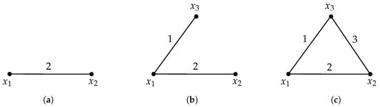
In our experiments, we construct undirected graphs with vertex and edge weights. The experimental results are categorized into three types based on the structure of the graphs, as shown in Figure 1. In Type 1 configuration with only two vertices, we set $\left(K\left(x_1\right),K\left(x_2\right)\right)=\left(0,-6.8\right)$. For other configurations, we fix $\left(K\left(x_1\right),K\left(x_2\right),K\left(x_3\right)\right)=(0,-6.8,-0.5)$ and observe how different values of $\kappa$ influence the variation of ${\lambda }_s$ as s increases. Here, $s\in (0,1)$ with a step size of 0.001.

Figure 1. Three types of graphs. (a) Type 1: The measure of vertex $x_1$ is 1, the measure of vertex $x_2$ is 0.5, and the weight of the edge $[x_1,x_2]$ is 2. (b) Type 2: The measures of vertices $x_1$, $x_2$ and $x_3$ are 1, 0.5 and 0.25, while the weights of edges $[x_1,x_3]$ and $[x_1,x_2]$ are 1 and 2. (c) Type 3: The measures of vertices $x_1$, $x_2$ and $x_3$ are 1, 0.5, and 0.25, while the weights of edges $[x_1,x_3]$, $[x_1,x_2]$, and $[x_2,x_3]$ are 1, 2, and 3.

5.2. Results

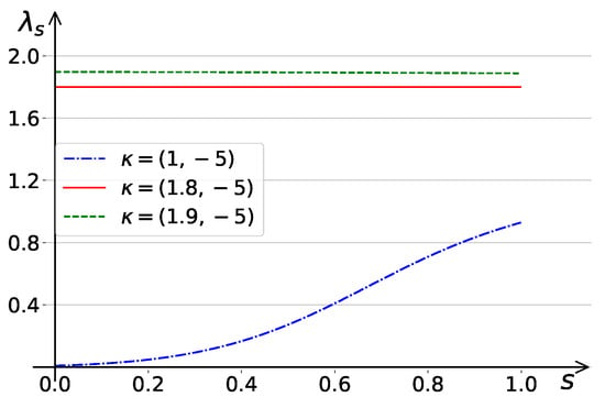
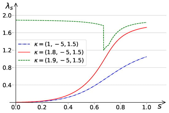
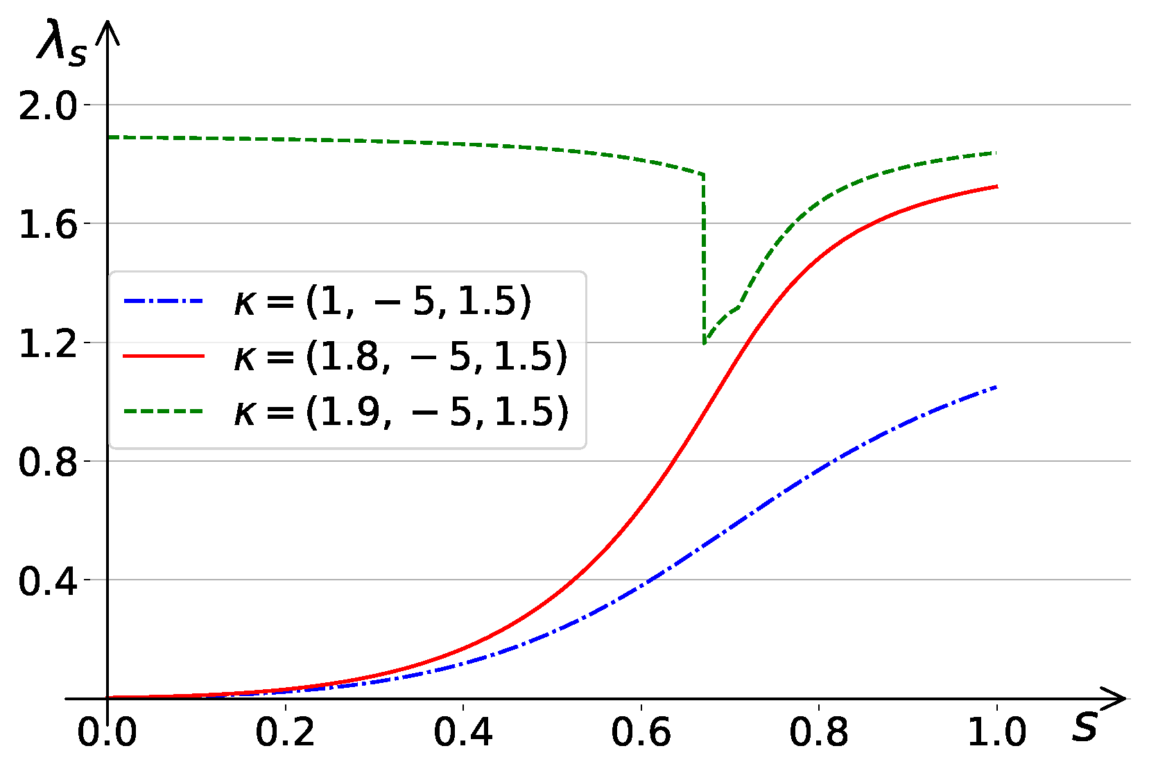
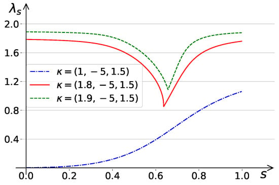
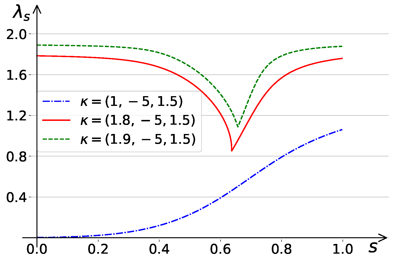
By visualizing the results, we obtained the outcomes shown in Figure 2, Figure 3 and Figure 4. It can be observed that, in all three configurations, the blue dash-dotted line consistently lies below the red solid line, while the green dashed line lies above the red solid line. This indicates that the first element of $\kappa$ has a positive impact on the value of ${\lambda }_s$ in our examples.

Figure 2. The variation of ${\lambda }_s$ as s ranges from 0 to 1 in Type 1 setting. Here, $K=\left(0,-6.8\right)$. The blue dash-dotted line represents the variation of ${\lambda }_s$ when $\kappa =(1,-5)$. The red solid line corresponds to $\kappa =(1.8,-5)$, while the green dashed line represents $\kappa =(1.9,-5)$.

Figure 3. The variation of ${\lambda }_s$ as s ranges from 0 to 1 in Type 2 setting. Here, $K=(0,-6.8,-0.5)$. The blue dash-dotted line represents the variation of ${\lambda }_s$ when $\kappa =(1,-5,1.5)$. The red solid line corresponds to $\kappa =(1.8,-5,1.5)$, while the green dashed line represents $\kappa =(1.9,-5,1.5)$.

Figure 4. The variation of ${\lambda }_s$ as s ranges from 0 to 1 in Type 3 setting. Here, $K=(0,-6.8,-0.5)$. The blue dash-dotted line represents the variation of ${\lambda }_s$ when $\kappa =(1,-5,1.5)$. The red solid line corresponds to $\kappa =(1.8,-5,1.5)$, while the green dashed line represents $\kappa =(1.9,-5,1.5)$.

In Figure 2, the blue dash-dotted line is strictly increasing, while the red solid line remains constant at 1.8. Although the green dashed line does not exhibit a clear trend in the figure, the numerical data show that it strictly decreases from 1.896942 at $s=0.001$ to 1.887452 at $s=0.999$.

In Figure 3, both the blue dash-dotted line and the red solid line are strictly increasing. The green dashed line, however, exhibits a significant gap at $s=0.671$, followed by a noticeable change in slope around $s=0.711$. These variations are likely the result of the combined effects of $\kappa$, s, and K. We believe that an intriguing direction for future research would be to investigate how individual elements of $\kappa$ and K influence the value of ${\lambda }_s$.

In Figure 4, the red solid line and the green dashed line exhibit local minima near $s=0.64$ and $s=0.66$, respectively. To the left of these minima, both lines are strictly decreasing, while to the right, they are strictly increasing. By examining the region $0.7<s<1$ in Figure 3 and Figure 4, we observe that the red solid line and the green dashed line demonstrate highly similar trends. An interesting avenue for future research could involve investigating how the weights of edges in the graph affect the threshold ${\lambda }_s$.

References

- Kazdan, J.; Warner, F. Curvature functions for compact 2-manifolds. Ann. Math. 1974, 99, 14–47. [Google Scholar] [CrossRef] [Scilit]
- Kazdan, J.; Warner, F. Curvature functions for open 2-manifolds. Ann. Math. 1974, 99, 203–219. [Google Scholar] [CrossRef] [Scilit]
- Chen, W.; Li, C. Gaussian curvature on singular surfaces. J. Geom. Anal. 1993, 3, 315–334. [Google Scholar] [CrossRef] [Scilit]
- Ding, W.; Jost, J.; Li, J.; Wang, G. The differential equation Δu = 8π − 8πheu on a compact Riemann Surface. Asian J. Math. 1997, 1, 230–248. [Google Scholar] [CrossRef] [Scilit]
- Ding, W.; Liu, J. A note on the problem of prescribing Gaussian curvature on surfaces. Trans. Amer. Math. Soc. 1995, 347, 1059–1066. [Google Scholar] [CrossRef]
- Borer, F.; Galimberti, L.; Struwe, M. “Large” conformal metrics of prescribed Gauss curvature on surfaces of higher genus. Comment. Math. Helv. 2015, 90, 407–428. [Google Scholar] [CrossRef] [Scilit]
- Struwe, M. The existence of surfaces of constant mean curvature with free boundaries. Acta Math. 1988, 160, 19–64. [Google Scholar] [CrossRef] [Scilit]
- Yang, Y.; Zhu, X. Prescribing Gaussian curvature on closed Riemann surface with conical singularity in the negative case. Ann. Acad. Sci. Fenn. Math. 2019, 44, 167–181. [Google Scholar] [CrossRef] [Scilit]
- Grigor, A.; Lin, Y.; Yang, Y. Kazdan-Warner equation on graph. Calc. Var. Partial Differ. Equ. 2016, 55, 92. [Google Scholar] [CrossRef] [Scilit]
- Ge, H. Kazdan-Warner equation on graph in the negative case. J. Math. Anal. Appl. 2017, 453, 1022–1027. [Google Scholar] [CrossRef] [Scilit]
- Ge, H. The p-th Kazdan-Warner equation on graphs. Commun. Contemp. Math. 2020, 22, 1950052. [Google Scholar] [CrossRef] [Scilit]
- Zhang, X.; Chang, Y. p-th Kazdan-Warner equation on graph in the negative case. J. Math. Anal. Appl. 2018, 466, 400–407. [Google Scholar] [CrossRef] [Scilit]
- Ge, H.; Jiang, W. Kazdan-Warner equation on infinite graphs. J. Korean Math. Soc. 2018, 55, 1091–1101. [Google Scholar]
- Keller, M.; Schwarz, M. The Kazdan-Warner equation on canonically compactifiable graphs. Calc. Var. Partial Differ. Equ. 2018, 57, 70. [Google Scholar] [CrossRef] [Scilit]
- Sun, L.; Wang, L. Brouwer degree for Kazdan-Warner equations on a connected finite graph. Adv. Math. 2022, 404, 108422. [Google Scholar] [CrossRef] [Scilit]
- Liu, S.; Yang, Y. Multiple solutions of Kazdan-Warner equation on graphs in the negative case. Calc. Var. Partial Differ. Equ. 2020, 59, 164. [Google Scholar] [CrossRef] [Scilit]
- Liu, Y.; Yang, Y. Topological degree for Kazdan-Warner equation in the negative case on finite graph. Ann. Glob. Anal. Geom. 2024, 65, 29. [Google Scholar] [CrossRef] [Scilit]
- Grigor, A.; Lin, Y.; Yang, Y. Yamabe type equations on graphs. J. Differ. Equ. 2016, 261, 4924–4943. [Google Scholar] [CrossRef] [Scilit]
- Grigor, A.; Lin, Y.; Yang, Y. Existence of positive solutions to some nonlinear equations on locally finite graphs. Sci. China Math. 2017, 60, 1311–1324. [Google Scholar] [CrossRef] [Scilit]
- Han, X.; Shao, M. p-Laplacian equations on locally finite graphs. Acta Math. Sin. (Engl. Ser.) 2021, 37, 1645–1678. [Google Scholar] [CrossRef] [Scilit]
- Hou, S.; Sun, J. Existence of solutions to Chern-Simons-Higgs equations on graphs. Calc. Var. Partial Differ. Equ. 2022, 61, 139. [Google Scholar] [CrossRef] [Scilit]
- Hua, B.; Wang, L. Dirichlet p-Laplacian eigenvalues and Cheeger constants on symmetric graphs. Adv. Math. 2020, 364, 106997. [Google Scholar] [CrossRef] [Scilit]
- Huang, H.; Wang, J.; Yang, W. Mean field equation and relativistic Abelian Chern-Simons model on finite graphs. J. Funct. Anal. 2021, 281, 109218. [Google Scholar] [CrossRef] [Scilit]
- Li, J.; Sun, L.; Yang, Y. Topological degree for Chern-Simons Higgs models on finite graphs. arXiv 2023, arXiv:2309.12024v1. [Google Scholar] [CrossRef] [Scilit]
- Riesz, M. L’intégrale de Riemann-Liouville et le problème de Cauchy pour l’équation des ondes. Bull. Soc. Math. Fr. 1939, 67, 153–170. [Google Scholar] [CrossRef] [Scilit]
- Biler, P.; Karch, G.; Woyczyński, W. Critical nonlinearity exponent and self-similar asymptotics for Lévy conservation laws. Ann. Inst. Henri Poincarè C Anal. Non Linéaire 2001, 18, 613–637. [Google Scholar]
- Caffarelli, L.; Valdinoci, E. Uniform estimates and limiting arguments for nonlocal minimal surfaces. Calc. Var. Partial Differ. Equ. 2011, 41, 203–240. [Google Scholar] [CrossRef] [Scilit]
- Iomin, A. Fractional Schrödinger equation in gravitational optics. Mod. Phys. Lett. A 2021, 36, 2140003. [Google Scholar] [CrossRef] [Scilit]
- Savin, O.; Valdinoci, E. Elliptic PDEs with fibered nonlinearities. J. Geom. Anal. 2009, 19, 420–432. [Google Scholar] [CrossRef] [Scilit]
- Maz’ya, V.; Verbitsky, I. The form boundedness criterion for the relativistic Schrödinger operator. Ann. Inst. Fourier 2004, 54, 317–339. [Google Scholar] [CrossRef] [Scilit]
- Meerschaert, M. Fractional Calculus, Anomalous Diffusion, and Probability; World Scientific Publishing Co. Pte. Ltd.: Hackensack, NJ, USA, 2012; pp. 265–284. [Google Scholar]
- Adams, R. Sobolev Spaces, Pure and Applied Mathematics; Academic Press: New York, NY, USA, 1975. [Google Scholar]
- Brezis, H.; Mironescu, P. Gagliardo-Nirenberg, composition and products in fractional Sobolev spaces. J. Evol. Equ. 2001, 1, 387–404. [Google Scholar] [CrossRef] [Scilit]
- Di Nezza, E.; Palatucci, G.; Valdinoci, E. Hitchhiker’s guide to the fractional Sobolev spaces. Bull. Sci. Math. 2012, 136, 521–573. [Google Scholar] [CrossRef] [Scilit]
- Kwaśnicki, M. Ten equivalent definitions of the fractional laplace operator. Fract. Calc. Appl. Anal. 2017, 20, 7–51. [Google Scholar] [CrossRef] [Scilit]
- Runst, T.; Sickel, W. Sobolev Spaces of Fractional Order, Nemytskij Operators, and Nonlinear Partial Differential Equations; De Gruyter Series in Nonlinear Analysis and Applications; Walter de Gruyter & Co.: Berlin, Germany, 1996; Volume 3. [Google Scholar]
- Ciaurri, Ó.; Roncal, L.; Stinga, P.; Torrea, J.; Varona, J. Nonlocal discrete diffusion equations and the fractional discrete Laplacian, regularity and applications. Adv. Math. 2018, 330, 688–738. [Google Scholar] [CrossRef] [Scilit]
- Keller, M.; Nietschmann, M. Optimal Hardy inequality for fractional Laplacians on the integers. Ann. Henri Poincaré 2023, 24, 2729–2741. [Google Scholar] [CrossRef] [Scilit]
- Lizama, C.; Roncal, L. Hölder-Lebesgue regularity and almost periodicity for semidiscrete equations with a fractional Laplacian. Discret. Contin. Dyn. Syst. 2018, 38, 1365–1403. [Google Scholar] [CrossRef] [Scilit]
- Wang, J. Eigenvalue estimates for the fractional Laplacian on lattice subgraphs. arXiv 2024, arXiv:2303.15766. [Google Scholar]
- Zhang, M.; Lin, Y.; Yang, Y. Fractional Laplace operator on finite graphs. arXiv 2024, arXiv:2403.19987. [Google Scholar]
- Zhang, M.; Lin, Y.; Yang, Y. Fractional Laplace operator and related Schrödinger equations on locally finite graphs. arXiv 2024, arXiv:2408.02902. [Google Scholar]
- Ciaurri, Ó.; Gillespie, T.; Roncal, L.; Torrea, J.; Varona, J. Harmonic analysis associated with a discrete Laplacian. J. Anal. Math. 2017, 132, 109–131. [Google Scholar] [CrossRef] [Scilit]
- Ciaurri, Ó.; Lizama, C.; Roncal, L.; Varona, J. On a connection between the discrete fractional Laplacian and superdiffusion. Appl. Math. Lett. 2015, 49, 119–125. [Google Scholar] [CrossRef] [Scilit]
- Ju, C.; Zhang, B. On fractional discrete p-Laplacian equations via Clark’s theorem. Appl. Math. Comput. 2022, 434, 127443. [Google Scholar] [CrossRef] [Scilit]
- Lizama, C.; Murillo-Arcila, M. On a connection between the N-dimensional fractional Laplacian and 1-D operators on lattices. J. Math. Anal. Appl. 2022, 511, 126051. [Google Scholar] [CrossRef] [Scilit]
- Tarasov, V. Exact discretization of fractional Laplacian. Comput. Math. Appl. 2017, 73, 855–863. [Google Scholar] [CrossRef] [Scilit]
- Ambrosetti, A.; Rabinowitz, P. Dual variational methods in critical point theory and applications. J. Funct. Anal. 1973, 14, 349–381. [Google Scholar] [CrossRef] [Scilit]
Disclaimer/Publisher’s Note: The statements, opinions and data contained in all publications are solely those of the individual author(s) and contributor(s) and not of MDPI and/or the editor(s). MDPI and/or the editor(s) disclaim responsibility for any injury to people or property resulting from any ideas, methods, instructions or products referred to in the content. |
© 2025 by the authors. Licensee MDPI, Basel, Switzerland. This article is an open access article distributed under the terms and conditions of the Creative Commons Attribution (CC BY) license (https://creativecommons.org/licenses/by/4.0/).