The Mechanism of Dissolution of Sparingly Soluble Salts—Application of a Novel Electrochemical Theory

Abstract

Although the dissolution of sparingly soluble salts is of interest to many fields, such as material science, dentistry, and geochemistry, the simplicity of these reactions provides its own motivation for study. Three features of these reactions are examined in this paper: (i) the unusual forms of the kinetic expression that have been used to describe their rates of reaction, (ii) the observation that the rate of dissolution is correlated with the potential difference across the solid-solution interface, and (iii) the observation of non-stoichiometric dissolution. Mechanistic descriptions of the kinetics of dissolution in current use do not account for all these factors, while the surface vacancy model does. In this paper, it is shown that linear kinetics arise from a symmetry of the rates of removal and deposition of anions and cations. On the other hand, non-linear kinetics arise from an asymmetry in the rates of removal and deposition of anions and cations. Because the surface vacancy model is an electrochemical model, the influence of potential difference on the rate of reaction is inherent to the model. A transient, or non-stationary state, version of the model is used to explain how non-stoichiometric dissolution arises.

1. Introduction

Dissolution is a fundamental reaction in chemistry with importance to a wide range of sciences and technologies. A knowledge of the kinetics and mechanism of dissolution reactions is therefore of fundamental interest, especially those salts whose rate is not limited by diffusion or under conditions in which diffusion is not the limiting factor. The dissolution of salts is both familiar and seemingly straight-forward: the salt reacts with water to form ionic species in solution. An example is the dissolution of gypsum, given in Equation (1).

$$CaS{O}_4·2H_{2}O(s)\rightleftharpoons C{a}^{2+}(aq)+S{O}_4^{2-}(aq)+2H_{2}O$$

(1)

The simplicity of reactions like this for the dissolution of sparingly soluble salts is their own justification for study. If these reactions can be shown to be described by a general mechanism, both our scientific knowledge and our confidence in its application improve dramatically [1]. Surprisingly, such a general mechanism has not been found for these simple reactions. Furthermore, dissolution reactions are important in diverse fields, from dentistry, where it is important in understanding tooth decay, to geochemistry, where dissolution controls the dissolved mineral content of fresh water, through to chemical processes, where leaching in hydrometallurgy is dissolution in industrial action.

The kinetics of dissolution of sparingly soluble salts are more likely to be controlled by the rate of the surface reaction than by the rate of film diffusion. Frequently, the empirical expression given in Equation (2) is invoked, which relates the rate of dissolution, r, to the degree of removal from saturation, 1 − S, in a non-linear manner.

$$r=k{\left(1-S\right)}^n$$

(2)

The symbol S is the saturation ratio defined as $C/C_s$, where C is the concentration of salt in the solution and C_s is the saturated concentration of salt in solution. The parameters are k, the rate constant, and n, the ‘saturation order’. The term ‘saturation order’ is used here instead of the term ‘order’ used in the literature to distinguish it from the term ‘order of reaction with respect to a reactant’ used in chemical kinetics, which has a different definition.

For gypsum, the value of n has been found to be one [2,3]. On the other hand, the value of n for the dissolution of AgCl, by the reaction given in Equation (3), has been found to be between 1.5 and 2 [4].

$$AgCl(s)\rightleftharpoons A{g}^{+}(aq)+C{l}^{-}(aq)$$

(3)

The values of n for other salt systems are given in Table 1. These values vary between linear, where n is equal to 1, and highly non-linear, where n is significantly greater than 1. It is this non-linearity that makes the scientific quest for a general mechanism challenging.

Table 1. Values for the ‘saturation order’, n, for the dissolution of sparingly soluble salts [5,6].

Salt	Saturation Order, n	Activation Energy, Ea, kJ/mol	Reference
PbSO4	2	10.0	[7]
BaSO4	2	24.7	[8]
SrSO4	2		[9]
AgCl	1.5–2.0	60	[4]
CaSO4·2H2O	1	20	[3]
Ag2CrO4	3		[10]
Ba(IO2)2	3	20	[11]
MgF2	2–3.5	86	[12]
CaF2	0.8–1.0	73	[13,14]
SrF2	1.7–3.8	72	[6]

The values not only vary between different salts but are also not constant for the same salt. This variability in the value of n for a particular salt and for different salt systems suggests that the empirical expression of Equation (2) does not adequately capture the kinetics of dissolution. This variability, in addition to the non-linearity, has made it surprisingly difficult to develop a general mechanism for these reactions.

Equation (2) is not the only rate expression used. The rate of dissolution of some salts has been correlated with the saturation state, Ω. Consider the dissolution of a generic salt, $A_a{B}_b$, in water by the reaction given in Equation (4).

$$M_m{A}_a\rightleftharpoons m{M}^{+a}+a{A}^{-m}$$

(4)

If the symbols $c_{-,eq}$ and $c_{+,eq}$ represent the concentrations of anions and cations at equilibrium, respectively, then the solubility product for this reaction can be expressed as Equation (5).

$$K_{sp}={(c_{+,eq})}^m{(c_{-,eq})}^a$$

(5)

At any condition removed from equilibrium or saturation, the saturation state is defined by Equation (6).

$$\mathsf{\Omega }={\displaystyle \frac{{c_{+}}^m{c_{-}}^a}{K_{sp}}}$$

(6)

The rate of dissolution is sometimes fitted to Equation (7) as an alternative to Equation (2). This equation acknowledges that the concentrations of anions and cations are not necessarily equivalent. The value of p will also be referred to as a saturation order, but bear in mind that p and n are not the same parameter.

$$r=k(1-\mathsf{\Omega }{)}^p$$

(7)

Like n, the reported values of p have a large range. For example, the value of p varies between 2 and 4 for calcite and aragonite, depending on the experimental conditions [15]. The critical weaknesses of Equation (2) are that (i) it does not represent the rate when the concentrations of anions and cations are not equal, and (ii) it does not reduce to the correct thermodynamic form yielding the solubility product when the rate is zero. These weaknesses are addressed by Equation (7); however, Equation (7) does not address the widespread values reported for the parameter p, nor does it provide any insight into why the kinetics are linear for some minerals, for example, gypsum, and non-linear for others, like AgCl.

Furthermore, there are additional features of dissolution reactions that are not captured by a kinetic expression or a rate equation. Two such features are (i) the non-stoichiometric dissolution of salts, and (ii) the potential difference that is developed across the solid-solution interface during dissolution due to the formation of surface charge. The presence of a surface charge during dissolution must influence the rate of removal of ions from the surface. A general mechanism must account for both features.

The preferential dissolution of one of the constituent ions from the surface is referred to as non-stoichiometric dissolution. This phenomenon has most commonly been observed in the dissolution of slow-dissolving minerals, such as those pertinent to chemical weathering. For example, Ruiz-Agudo et al. [16] described the preferential removal of calcium from wollastonite, CaSiO₃.

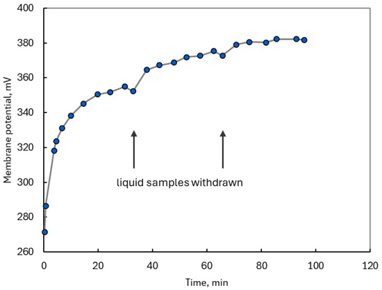
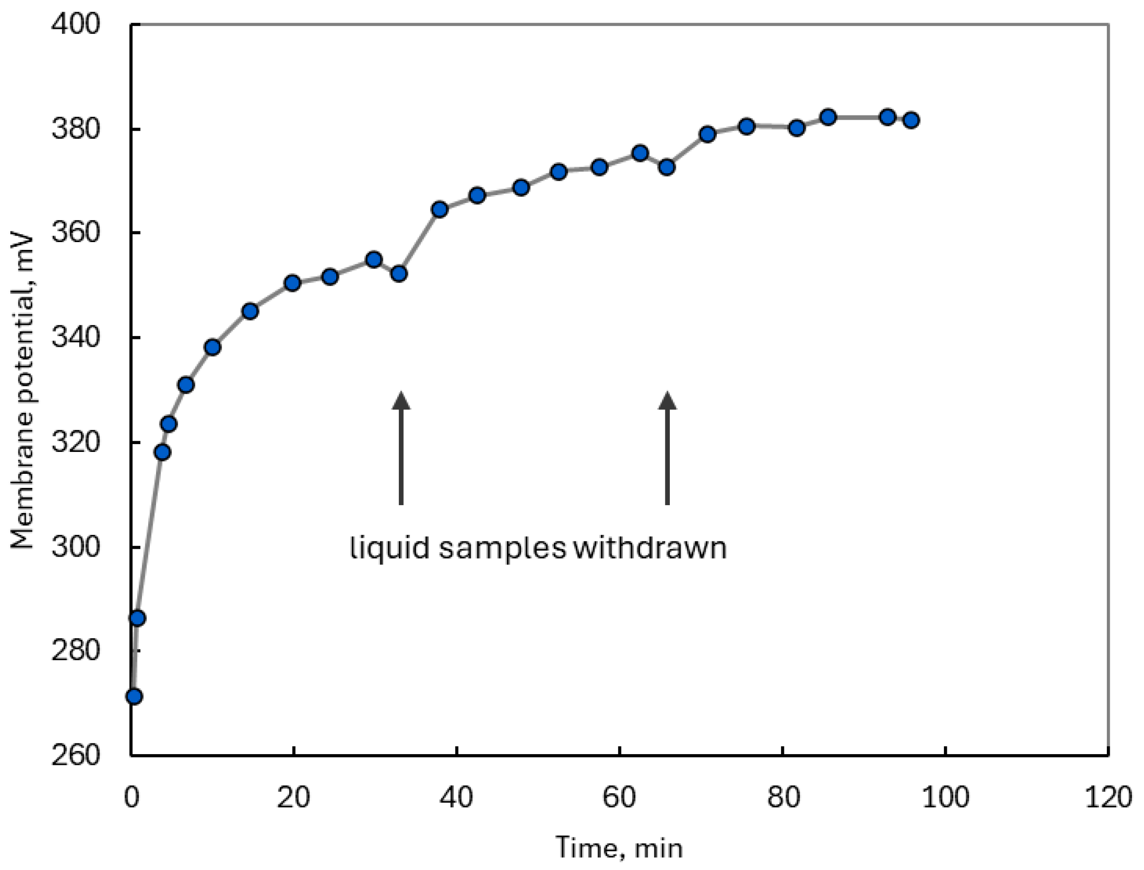
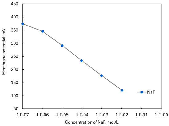
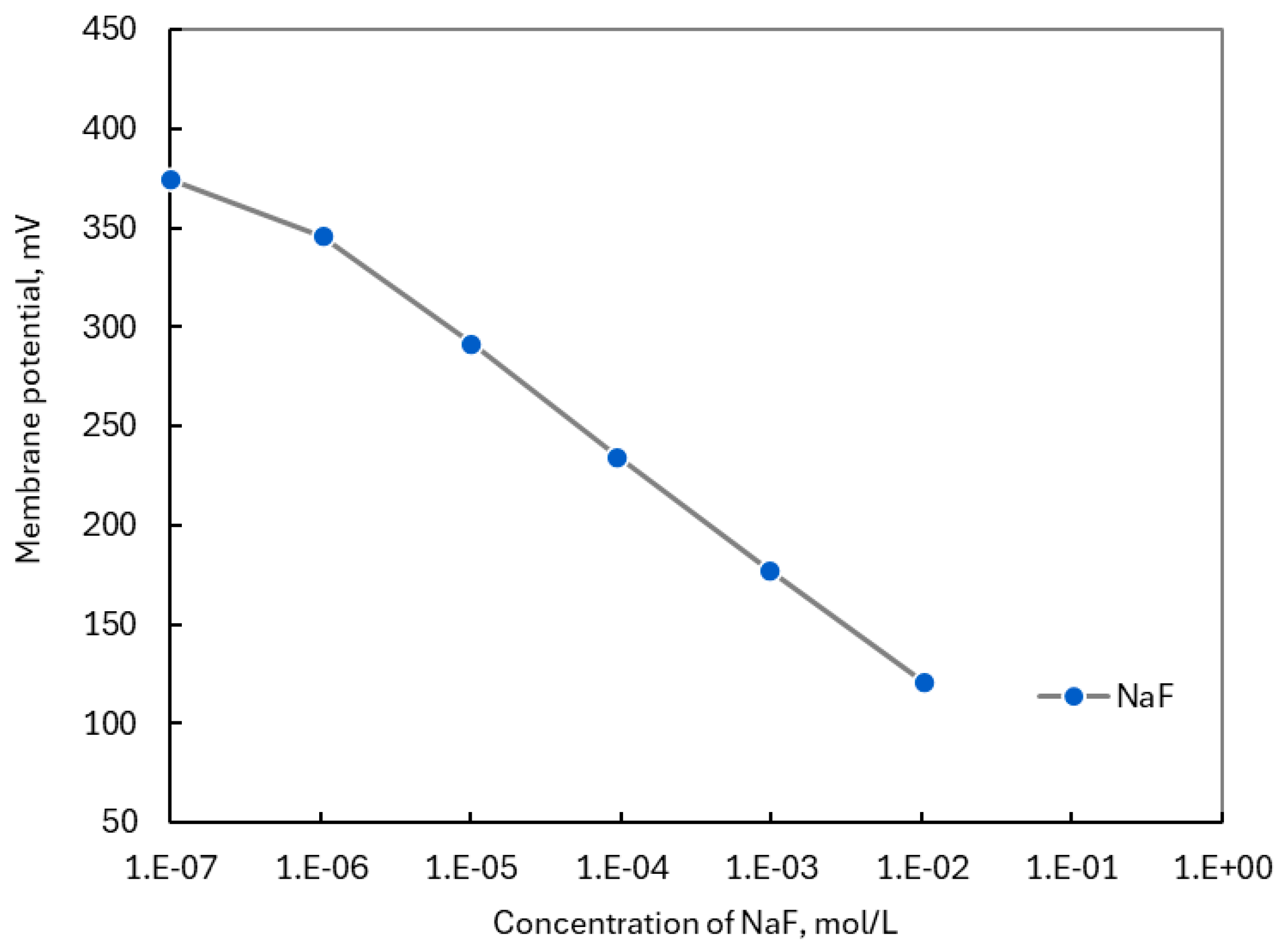
Tani et al. [17] expected the stoichiometric removal of lanthanum and fluoride in their investigation of the dissolution of lanthanum fluoride, LaF₃. However, they found that only fluoride ions were removed while the concentration of lanthanum in solution was below detection limits. Tani et al. [17] reasoned that the preferential removal of fluoride ions would leave positively charged vacancies on the surface of LaF₃. To test this hypothesis, they measured the membrane potentials of a LaF₃ single crystal. The results of these tests are shown in Figure 1, confirming that a change in the membrane potential of LaF₃ occurred in the period after the immersion of the electrode into solution. They also demonstrated that this change in potential is a function of the concentration of fluoride ions in solution, as shown in Figure 2. Therefore, the results reported by Tani et al. [17] demonstrate that non-stoichiometric dissolution and interfacial surface potential are related.

Figure 1. The change in the membrane potential of a LaF₃ single crystal with time in a solution of 0.1 M NaNO₃ and 0.01 M acetate buffer at pH 5.2. Measurements are indicated by the points. The solutions were changed for a fresh solution at the times marked by the arrows. The removed solutions were found to contain fluoride ions, but the lanthanum ions were below detection limits. Data from Tani et al. [17].

Figure 2. The effect of fluoride ions on the membrane potential of LaF₃. Data from Tani et al. [17].

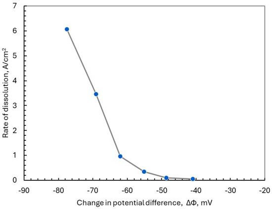
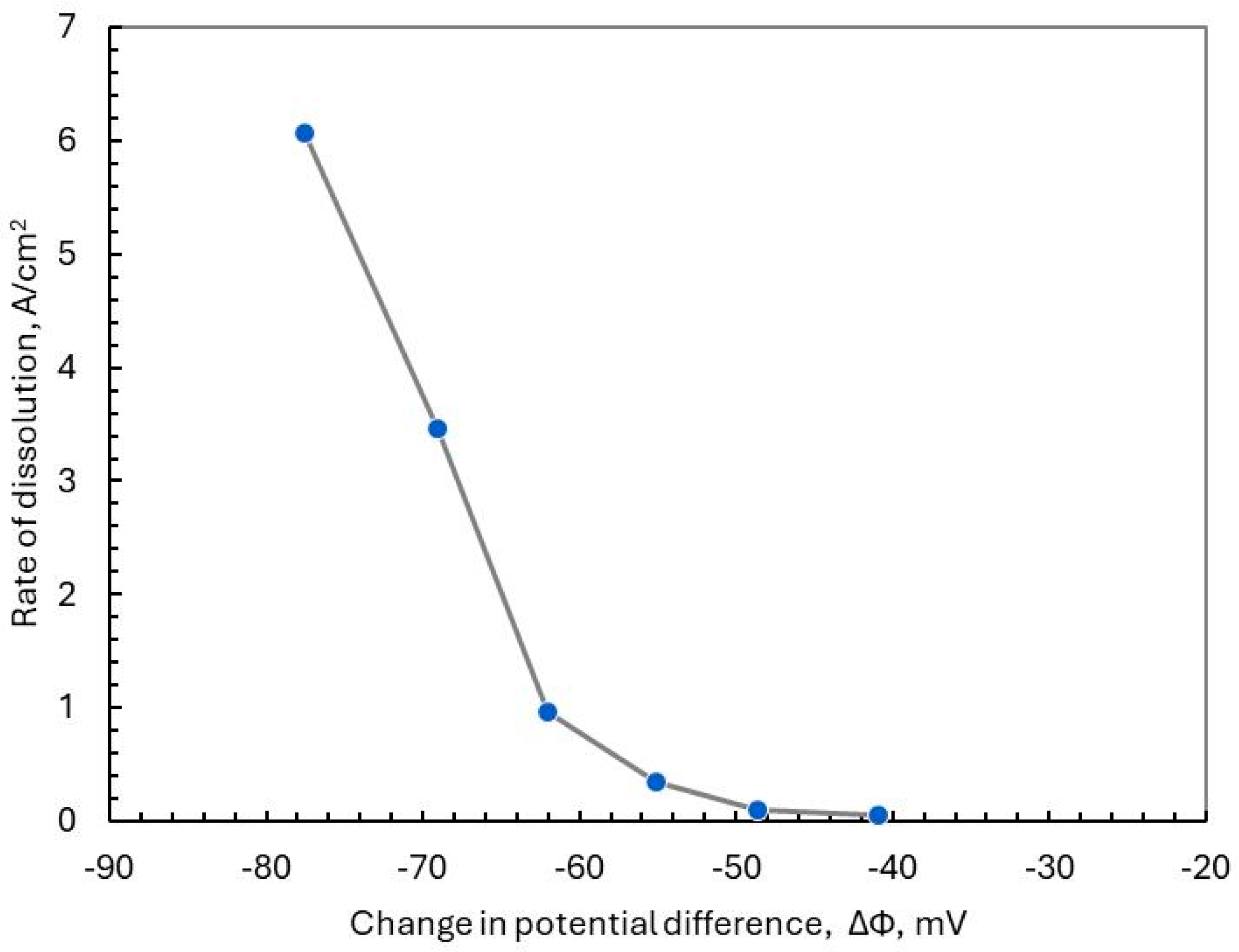
Other dissolution systems have been shown to develop an interfacial potential difference. Ibl et al. [18] demonstrated that the membrane potential of NaCl, KCl, and K Na-tartrate is correlated with the conditions of under- and over-saturation, leading to dissolution and crystallization, respectively. Jaenicke [19] correlated the rate of dissolution with the membrane potential of AgCl. These early results of Jaenicke [19] are shown in Figure 3.

Figure 3. The relationship between change in membrane potential and rate of reaction (expressed as an equivalent current). Data from Jaenicke [19].

Several different approaches to developing an understanding of the dissolution of sparingly soluble salts have been made [20]. Probably the most accepted model currently is the physical model based on the removal of ions from weak points on the crystal face. To this effect, the screw dislocation model developed for crystallization from the vapor phase has been adapted to describe dissolution [6,21]. This model predicts a parabolic dependence on the saturation ratio at low deviations from equilibrium and a linear dependence at high deviations from equilibrium.

While the screw dislocation model and variants built on that central idea can be adapted to fit the measured kinetics of dissolution [6], it fails to provide the correct thermodynamic form at zero rate, it fails to account for the common ion effect, and it fails to provide any insight into the phenomena of non-stoichiometric dissolution and the development of an interfacial potential difference as a result of dissolution [20].

Another approach has been pioneered by Davies and Jones [22]. They envisaged a layer of ions adsorbed or adherent to the surface of the salt that was in equilibrium with the surface. Their hypothesis was that the adsorbed layer was such that if an anion, say, entered the layer, it caused disequilibrium, resulting in the deposition of an anion on the surface. In this way, the adsorption layer controlled the rate of reaction. Their derivation produced an expression that accounted for chemical equilibrium and was second order (n = 2), resulting in widespread early adoption by other researchers. However, this model is somewhat artificial, as pointed out by the originator [23] and others [20,24].

In common with the screw dislocation model and variants built upon it, the adsorption layer model of Davies and Jones [22] has no explanation for non-stoichiometric dissolution. Thus, there is no general mechanism for the kinetics of dissolution of sparingly soluble salts. Linge [20] suggested that an electrochemical approach might yield such a mechanism. At the time of the survey by Linge [20], several electrochemical approaches had been followed, including that of Jaenicke [19] and Vermilyea [25]. However, while these models are broadly in line with the work presented here, they did not begin with a model of the surface that would allow them to derive an understanding of non-stoichiometric dissolution, nor did they derive a rate expression that covered the entire range of conditions from equilbrium through to dissolution in a solution that was free of the salt in question or any of its constituent ions.

In summary, a more comprehensive understanding of the dissolution of sparingly soluble salts requires an explanation for the following three features:

(i)

Kinetics: The rate of dissolution is correlated empirically with the undersaturation. Values of the ‘saturation order’ range from 1 to 4; they are not constant for the same salt, and they are not necessarily constant for the full range of saturation (S from 0 to 1).

(ii)

Surface charge and potential difference: Salt dissolution is correlated with the potential difference across the solid-solution interface. This occurs in the absence of other ions that might adsorb to the surface, indicating that it is an intrinsic property of the salt, a phenomenon sometimes referred to as ‘self-ionization’ of the surface.

(iii)

Non-stoichiometric dissolution: The rate of dissolution of sparingly soluble salts is known to sometimes favor one of the constituent ions. An extreme example is that of LaF₃, in which the dissolution of only fluoride ions from the surface was detected.

The purpose of this paper is to demonstrate that the electrochemical mechanism developed for NaCl (halite) and CaSO₄·2H₂O (gypsum) applies to sparingly soluble salts [26,27]. The specific aim is to demonstrate that this mechanism describes all the features of dissolution reactions of sparingly soluble salts mentioned above, that is, it describes the reported data for linear and parabolic kinetics while providing insight into the conditions when different ‘saturation orders’ might arise, it provides an explanation for non-stoichiometric dissolution and it provides an explanation for the development of the interfacial potential difference.

2. Electrochemical Mechanism of Dissolution

Crundwell [1,28,29,30,31,32,33] described a model for the acid-base dissolution of minerals that was termed the ‘surface vacancy model’. The surface vacancy mechanism has been applied to the dissolution of a soluble salt (halite, NaCl), and an insoluble salt (gypsum, CaSO₄·2H₂O) [26,27]. Although this model has been presented in these other works, it is expounded here for completeness and clarity.

The description of the physical model is discussed next, following which a mathematical description is developed.

2.1. Physical Description of the Electrochemical Mechanism

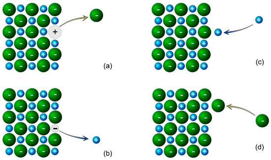
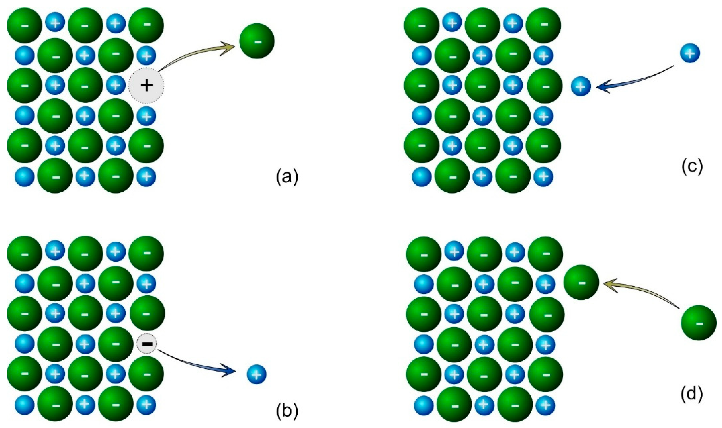
Consider a salt that consists of $M^{z+}$ and $A^{z-}$ ions dissolving according to the reaction given in Equation (4). As these constituent ions depart individually from the surface of the salt they leave a surface vacancy on the surface. This is illustrated in Figure 4a,b. This surface vacancy represents an uncompensated charge, giving the model its name.

Figure 4. Dissolution occurs by the separate removal of (a) anions and (b) cations from the surface leaving a charge of the opposite sign on the surface due to the surface vacancy. Deposition of (c) cations and (d) anions onto the surface results in the adding a charge of the same sign onto the surface [26].

The independent removal of anions and cations from the surface for the overall reaction given by Equation (4) can be represented by Equations (8) and (9) for the removal of cations and anions from the surface:

$$\left.\equiv \right|M\hspace{1em}\rightleftharpoons \hspace{1em}{M}^{z+}(aq)\hspace{1em}+\hspace{1em}{\left.\equiv \right|}^{z-}$$

(8)

$$\left.\equiv \right|A\hspace{1em}\rightleftharpoons \hspace{1em}{A}^{z-}(aq)\hspace{1em}+\hspace{1em}{\left.\equiv \right|}^{z+}$$

(9)

The symbol $\left.\equiv \right|M$ represents an M ion anywhere on the surface, and the symbol ${\left.\equiv \right|}^{z-}$ represents a negatively charged vacancy on the surface. The model does not distinguish between sites on the surface plane, at edges, at kinks, at ledge positions, or any other sites. The surface concentration of vacancies is not described by an isotherm, and vacancies are distributed evenly over the dissolving surface. This mechanism is sometimes referred to as ‘self-ionization’ (see Grimley [34]) because the surface becomes charged in the absence of adsorbable ions in the electrolyte.

The uncompensated charge on the surface results in a potential difference across the solid-solution interface and the formation of an electrified double layer. The measured membrane potentials given in Figure 1 and Figure 2 are in the range of tens to hundreds of millivolts. The interfacial capacitance is typically found to be in the range of 0.01 to 0.2 F/m² [35]. A reasonable value might be 0.05 F/m². A change in the potential difference at the surface of 0.1 V corresponds to an increase in the charge of 0.1 V × 0.05 F/m² = 0.005 C/m² [35,36]. This increase in charge is correspondingly caused by an increase in the concentration of anion vacancies, say, over cation vacancies of (0.005 C/m²)/(96,500 C/mol) = 5.2 × 10⁻⁸ mol/m² or about 10¹⁴ ions/m², assuming a single charge on each of the vacancies. Since the total surface concentration of constituent ions of the salt is between 10⁻³ and 10⁻⁴ mol/m² (10¹⁹ or 10²⁰ ions/m²) based on the range of ionic radius [37,38], the vacancy concentration is several orders of magnitude lower than the total surface concentration. For an ion of radius 0.5 Å, the surface area per mol of surface ions is 1/(0.5 Å × 0.5 Å × 6.02 × 10²³ ions/mol) = 6.4 × 10⁻⁴ mols/m². Thus, a very low concentration of surface vacancies, 1 in approximately 10⁴, has a significant impact on the interfacial potential difference.

If there are dissolved species in solution, most of the potential difference occurs across the narrow Helmholtz layer, which is the distance between the surface and the plane of closest approach of a hydrated ion. Thus, the potential difference that is referred to by the phrase ‘interfacial potential difference’ is that across the Helmholtz layer. The thickness of the Helmholtz layer is of the order of the size of a water molecule, about 3 × 10⁻¹⁰ m [39]. Therefore, the field strength is 0.1 V/3 × 10⁻¹⁰ = 3 × 10⁹ V/m. This electrical field strength exerts a significant force on the removal and deposition of ions during dissolution.

Importantly, this means that the rates of removal and deposition of both anions and cations depend on the potential difference across the interface, which in turn is directly dependent on the net charge that the ions leave behind when they are removed. Therefore, the individual steps that are given in Equations (8) and (9) are electrochemical in nature, albeit in the form of the ionic transfer rather than electron transfer [40]. Furthermore, the rates of departing and depositing cations and anions are independent of one another but coupled by their mutual dependence on the interfacial potential difference.

The mechanism given by Equations (8) and (9) anticipates two elementary reaction steps in the forward direction, one for each type of ion. In the reverse direction, there are a further two elementary steps, leading to a mechanism of four elementary reaction steps for dissolution conditions close to equilibrium.

2.2. Mathematical Formulation of the Electrochemical Mechanism

The net charge on the surface of the salt, ${\sigma }_0$, developed by surface vacancies due to the partial reactions of Equations (8) and (9), is given by Equation (10) [35,41,42]:

$${\sigma }_0=F(z_{+}{\mathsf{\Gamma }}_{+}-z_{-}{\mathsf{\Gamma }}_{-})$$

(10)

The meaning of the symbols is as follows: F represents the Faraday constant (C/mol), $z_{-}$ and $z_{+}$ represent the absolute values of the ionic charges, while ${\mathsf{\Gamma }}_{-}$ and ${\mathsf{\Gamma }}_{+}$ represent the surface concentrations of the anionic and cationic vacancies, respectively. The term in brackets on the right-hand side of Equation (10) is referred to as the excess surface charge.

Taking derivatives of Equation (10) with respect to time yields Equation (11).

$${\displaystyle \frac{d{\sigma }_0}{dt}}=F(z_{+}{\displaystyle \frac{d{\mathsf{\Gamma }}_{+}}{dt}}-z_{-}{\displaystyle \frac{d{\mathsf{\Gamma }}_{-}}{dt}})$$

(11)

The rate of change in the surface concentration of cationic vacancies is equal to the rate of removal of anionic species, that is, $d{\mathsf{\Gamma }}_{+}/dt$ is equal to $r_{-}$, and similarly, $d{\mathsf{\Gamma }}_{-}/dt$ is equal to $r_{+}$. Consequently, using these relationships yields Equation (12).

$${\displaystyle \frac{d{\sigma }_0}{dt}}=F(z_{+}{r}_{-}-z_{-}{r}_{+})$$

(12)

The potential difference across the interface is related to the surface charge by the interfacial capacitance, $C_d$, by Equation (13) [35,39].

$$\Delta \varphi ={\displaystyle \frac{{\sigma }_0}{C_d}}$$

(13)

The combination of Equation (12) with Equation (13) yields an expression, Equation (14), for the change in potential as the rate of removal of anions and cations changes.

$${\displaystyle \frac{d\Delta \varphi }{dt}}={\displaystyle \frac{F}{C_d}}\left(z_{+}{r}_{-}-z_{-}{r}_{+}\right)$$

(14)

Importantly, Equation (14) is consistent with the observation by Ibl et al. [18] and Jaenicke [19] that their measurements of the changes in potential difference were correlated with the rate of dissolution of the salt. Equation (14) is also the key to unlocking the mechanism of non-stoichiometric dissolution. If there is a mismatch between the rates of removal of anions and cations, the surface charge and the interfacial potential difference will change according to Equations (12) and (14).

Once the surface charge and the potential difference stabilize, the rate of dissolution stabilizes. This is referred to as a stationary state. The condition for stable dissolution is therefore that $d{\sigma }_0/dt=0$ or equivalently $d\Delta \varphi /dt=0$. The application of this condition to Equation (14) leads to Equation (15):

$${\displaystyle \frac{r_{-}}{z_{-}}}={\displaystyle \frac{r_{+}}{z_{+}}}$$

(15)

Equation (15) is simply a statement of stoichiometry. This means that the condition for stoichiometric dissolution is that there is no change in interfacial potential difference with time, that is, $d\Delta \varphi /dt$ is zero. Stated differently but equivalently, the time rate of change in the surface charge, $d{\sigma }_0/dt$, is zero. The condition for stoichiometric dissolution is not that the surface is neutrally charged, as assumed by most work in the literature, but that a stationary state occurs where the change in the surface charge with time is zero. Stoichiometric dissolution only occurs once the surface charge and potential difference stabilize and the derivative term in Equation (14) approaches zero. At this point, the overall rates of removal of anions and cations are equal.

If the rate of removal of the cations is not stoichiometrically proportional to the rate of removal of anions, the surface charge will change with time according to Equation (14) until the stoichiometric dissolution condition is met.

The rate of removal of anions and cations from the surface to the solution is an electrochemical ion-transfer reaction dependent on the potential difference across the interface [19,25,26]. The electrochemical rate expression includes the detachment of the ion from its bonding site on the surface, its hydration, and its transfer to the solution, all of which are accounted for in the phenomenological expression for electrochemical kinetics. The rate of removal of anions, $r_{-}$, and cations, $r_{+}$, in the forward and reverse directions, is given by the electrochemical expressions of Equations (16) and (17), respectively.

$$r_{-}={\overrightarrow{k}}_{-}\exp \left(-z_{-}(1-{\alpha }_{-})F\Delta \varphi /RT\right)-{\overleftarrow{k}}_{-}{c}_{-}\exp \left(z_{-}{\alpha }_{-}F\Delta \varphi /RT\right)$$

(16)

$$r_{+}={\overrightarrow{k}}_{+}\exp \left(z_{+}{\alpha }_{+}F\Delta \varphi /RT\right)-{\overleftarrow{k}}_{+}{c}_{+}\exp \left(-z_{+}(1-{\alpha }_{+})F\Delta \varphi /RT\right)$$

(17)

The symbols are defined as follows: R represents the gas constant (J/mol/K), T the temperature (K), $\Delta \varphi$ is the potential difference across the Helmholtz layer (V), $k_{-}$ and $k_{+}$ are the electrochemical rate constants for the anion and the cation, $z_{-}$ and $z_{+}$ are the absolute charges on the anion and cation, and ${\alpha }_{-}$ and ${\alpha }_{+}$ are the charge transfer coefficients for the anion and cation. The vinculum arrows on the rate constants k indicate the forward (dissolution) and reverse (deposition) directions of the reaction for each ion.

There is a difference between Equations (16) and (17) and the corresponding expressions used by Crundwell [1,33]. The values of the ionic charge, $z_{-}$ and $z_{+}$, have been included in Equations (16) and (17), whereas Crundwell [1,33] proposed an alternative model, mainly aimed at acid-base reactions, in which they were not included. This ionic form is used as a hypothesis of this work because the bonding of the sparingly soluble is ionic in nature.

Thus, the model consists of Equations (16) and (17) with either Equation (14) for the description of non-stoichiometric dissolution or Equation (15) for stoichiometric dissolution at the stationary conditions.

Simplifying assumptions are required to obtain an analytical solution of Equations (15)–(17). Since the values of the charge transfer coefficients are usually between 0.4 and 0.6 [39], the assumption is made that ${\alpha }_{+}\approx {\alpha }_{-}\approx \raisebox{1ex}{$1$}\!\left/ \!\raisebox{-1ex}{$2$}\right.$. Furthermore, the discussion is restricted to equimolar salts, so that $z_{+}=z_{-}$ to allow for an analytical solution. Under these conditions, Equations (16) and (17) can be made more compact by the substitution $y=z_{-}F\Delta \varphi /2RT=z_{+}F\Delta \varphi /2RT$. Substitution of this form of Equations (16) and (17) into Equation (15), which is the condition for stoichiometric dissolution, yields Equation (18).

$${\overrightarrow{k}}_{-}\exp (-y)-{\overleftarrow{k}}_{-}{c}_{-}\exp (y)={\overrightarrow{k}}_{+}\exp (y)-{\overleftarrow{k}}_{+}{c}_{+}\exp (-y)$$

(18)

Solving Equation (18) for $\exp (y)$ yields Equation (19).

$$\exp (2y)={\displaystyle \frac{{\overrightarrow{k}}_{-}+{\overleftarrow{k}}_{+}{c}_{+}}{{\overrightarrow{k}}_{+}+{\overleftarrow{k}}_{-}{c}_{-}}}$$

(19)

This expression describes the potential difference across the Helmholtz layer due to dissolution under the conditions of stoichiometric dissolution.

Equation (19) indicates that the potential is dependent on the concentrations of $M^{z+}$ and $A^{z-}$ during dissolution or crystallization [34,35]. In other words, they are potential-determining ions. Equation (19) is not Nernstian; however, if the conditions that $c_{+}\gg {\overrightarrow{k}}_{-}/{\overleftarrow{k}}_{+}$ and $c_{-}\gg {\overrightarrow{k}}_{+}/{\overleftarrow{k}}_{-}$ are both met, then Equation (19) is Nernstian. In other words, Equation (19) is Nernstian close to equilibrium, or, as in the case of LaF₃ shown in Figure 1, the rate constants in the forward direction are much smaller than those in the deposition direction.

Substitution of Equation (19) into either Equation (16) or Equation (17) yields, after some algebraic manipulation, Equation (20), the expression for the rate of dissolution. Since the rates of removal of anions and cations are equal at the stationary state defined by Equation (15), $r_{-}$ is equal to $r_{+}$, and this is simply the rate of dissolution, $\overrightarrow{r}$.

$$\overrightarrow{r}={\displaystyle \frac{{\overrightarrow{k}}_{+}{\overrightarrow{k}}_{-}-{\overleftarrow{k}}_{+}{\overleftarrow{k}}_{-}{c}_{+}{c}_{-}}{{\left({\overrightarrow{k}}_{-}+{\overleftarrow{k}}_{+}{c}_{+}\right)}^{\raisebox{1ex}{$1$}\!\left/ \!\raisebox{-1ex}{$2$}\right.}{\left({\overrightarrow{k}}_{+}+{\overleftarrow{k}}_{-}{c}_{-}\right)}^{\raisebox{1ex}{$1$}\!\left/ \!\raisebox{-1ex}{$2$}\right.}}}$$

(20)

By setting the rate to zero in Equation (20), we find that the equilibrium constant or solubility product is given by Equation (21).

$$K_{sp}={\displaystyle \frac{{\overrightarrow{k}}_{+}{\overrightarrow{k}}_{-}}{{\overleftarrow{k}}_{+}{\overleftarrow{k}}_{-}}}=c_{+,eq}{c}_{-,eq}$$

(21)

The number of unknown parameters in the rate expression given by Equation (20) is reduced to two by introducing Equation (21) for the equilibrium constant. After some algebraic rearrangement, the rate expression for ionic solids is given in Equation (22).

$$\overrightarrow{r}={\displaystyle \frac{k_1\left(1-c_{+}{c}_{-}/K_{sp}\right)}{{\left(1+k_2{c}_{+}\right)}^{\raisebox{1ex}{$1$}\!\left/ \!\raisebox{-1ex}{$2$}\right.}{\left(1+c_{-}/K_{sp}{k}_2\right)}^{\raisebox{1ex}{$1$}\!\left/ \!\raisebox{-1ex}{$2$}\right.}}}$$

(22)

The rate constant $k_1$ is given by ${\left({\overrightarrow{k}}_{+}{\overrightarrow{k}}_{-}\right)}^{\raisebox{1ex}{$1$}\!\left/ \!\raisebox{-1ex}{$2$}\right.}$ and $k_2$ is given by ${\overleftarrow{k}}_{+}/{\overrightarrow{k}}_{-}$.

Equation (22) can be expressed in terms of the saturation state, Ω, as shown in Equation (23).

$$\overrightarrow{r}={\displaystyle \frac{k_1\left(1-\mathsf{\Omega }\right)}{{\left(1+k_2{c}_{+}\right)}^{\raisebox{1ex}{$1$}\!\left/ \!\raisebox{-1ex}{$2$}\right.}{\left(1+c_{-}/K_{sp}{k}_2\right)}^{\raisebox{1ex}{$1$}\!\left/ \!\raisebox{-1ex}{$2$}\right.}}}$$

(23)

The form of the numerator in Equation (23) resembles the simplistic form suggested by Equation (7) with the ‘saturation order’ of one. The non-linearity that Equation (7) captures by empirically introducing the ‘saturation order’ p in Equation (7) is described theoretically by the unusual denominator in Equation (23).

While Equation (23) is written as a function of the saturation state, Ω, it is for comparison purposes only. This form is not useful or practical since Ω is not the independent variable. Rather, the correct independent kinetic variables are the concentrations of anions and cations, and the form of the model that should be applied to experimental data is Equation (22).

2.3. Limiting Cases

The functional form derived for the rate of dissolution given by Equations (22) and (23) is not anticipated by any other theory of dissolution. Because of its unfamiliarity, it is necessary to explore the limiting cases.

2.4. Dissolution Far from Equilibrium

At conditions far from equilibrium, the concentrations of $c_{+}$ and $c_{-}$ are small. Setting the terms in Equation (22) that contain these concentrations to zero, Equation (22) yields the limiting form given by Equation (24).

$$\overrightarrow{r}={\left({\overrightarrow{k}}_{+}{\overrightarrow{k}}_{-}\right)}^{\raisebox{1ex}{$1$}\!\left/ \!\raisebox{-1ex}{$2$}\right.}=k_1$$

(24)

Far from equilibrium and in the absence of Nernst film diffusion, the rate of dissolution is dependent on temperature alone.

2.5. Growth Far from Equilibrium

The rate of growth is the reverse of dissolution. The expression for the rate of growth can be obtained by returning to Equations (16) and (17) using only the terms describing the reverse reaction and then following the same method as that used to get to Equation (20). Alternatively, if it is assumed that the rate in the forward direction is much slower than in the reverse direction, that is, ${\overrightarrow{k}}_{+}{\overrightarrow{k}}_{-}$ is much less than ${\overleftarrow{k}}_{+}{\overleftarrow{k}}_{-}{c}_{+}{c}_{-}$ in Equation (20), and simplifying, the same result can be achieved. Therefore, far from equilibrium, the rate is given by Equation (25) for ionic solids in which the ratio of $z_{+}$ to $z_{-}$ is one.

$$\overleftarrow{r}={\left({\overleftarrow{k}}_{+}{\overleftarrow{k}}_{-}{c}_{+}{c}_{-}\right)}^{\raisebox{1ex}{$1$}\!\left/ \!\raisebox{-1ex}{$2$}\right.}=k_{-1}{\left(c_{+}{c}_{-}/K_{sp}\right)}^{\raisebox{1ex}{$1$}\!\left/ \!\raisebox{-1ex}{$2$}\right.}=k_{-1}{\mathsf{\Omega }}^{\raisebox{1ex}{$1$}\!\left/ \!\raisebox{-1ex}{$2$}\right.}$$

(25)

2.6. Extension to Non-Equimolar Salts

The mathematical development of the model was restricted earlier in this section to equimolar salts so that an analytical solution could be obtained. This restriction can be lifted, but at this stage, it is not known if an analytical solution is possible, because the equation corresponding to Equation (18) yields higher-order polynomials in $\exp (y)$ for which analytical solutions are more complex than presented here. This is an area of ongoing investigation, albeit an algebraic exercise rather than model development.

3. Results

The proposed mechanism for the dissolution of sparingly soluble salts, Equation (22), is consistent with chemical thermodynamics, since it yields the equilibrium expression when the rate is set to zero, and it accounts for the common ion effect, because it is dependent on the concentrations of each of the constituent ions.

A comprehensive mechanism must describe the kinetics that are both linear (saturation orders of 1) and non-linear (saturation orders of between 1 and 4), and account for non-stoichiometric dissolution and surface charge that gives rise to the interfacial potential difference.

3.1. Linear Kinetics, Saturation Order of One

Generally, the kinetics of dissolution are non-linear with respect to the undersaturation 1 − S, with values of the ‘saturation order’ n greater than one. An interesting case is that for some salts, the value of n is one. CaSO₄·2H₂O, NaCl, and KCl all display linear kinetics under conditions in which surface reaction controls the rate of dissolution [3,26,43]. Despite these seemingly simple kinetics, deriving a kinetic expression is difficult because S is defined in terms of the concentration of the salt rather than in terms of the concentrations of anions and cations in solution [26].

Consider dissolution under the condition where the concentrations of anions and cations in solution are equal (no common ions in solution), so that $c_{+}=c_{-}=c$. This allows Equation (22) to be written as Equation (26).

$$\overrightarrow{r}={\displaystyle \frac{k_1\left(1-c^2/K_{sp}\right)}{{\left(1+k_{2}c\right)}^{\raisebox{1ex}{$1$}\!\left/ \!\raisebox{-1ex}{$2$}\right.}{\left(1+c/K_{sp}{k}_2\right)}^{\raisebox{1ex}{$1$}\!\left/ \!\raisebox{-1ex}{$2$}\right.}}}$$

(26)

If it is assumed that $K_{sp}={(1/k_2)}^2$ is a mathematical hypothesis, then the denominator can be written in a symmetrical form, as given in Equation (27).

$$\overrightarrow{r}={\displaystyle \frac{k_1\left(1-c^2/K_{sp}\right)}{{\left(1+c/K_{sp}^{\raisebox{1ex}{$1$}\!\left/ \!\raisebox{-1ex}{$2$}\right.}\right)}^{\raisebox{1ex}{$1$}\!\left/ \!\raisebox{-1ex}{$2$}\right.}{\left(1+c/K_{sp}^{\raisebox{1ex}{$1$}\!\left/ \!\raisebox{-1ex}{$2$}\right.}\right)}^{\raisebox{1ex}{$1$}\!\left/ \!\raisebox{-1ex}{$2$}\right.}}}$$

(27)

The numerator of Equation (27) can be factored to yield Equation (28), which can be simplified to yield Equation (29) since $S=c/{K_{sp}}^{\raisebox{1ex}{$1$}\!\left/ \!\raisebox{-1ex}{$2$}\right.}$.

$$\overrightarrow{r}={\displaystyle \frac{k_1\left(1-c/{K_{sp}}^{\raisebox{1ex}{$1$}\!\left/ \!\raisebox{-1ex}{$2$}\right.}\right)\left(1+c/{K_{sp}}^{\raisebox{1ex}{$1$}\!\left/ \!\raisebox{-1ex}{$2$}\right.}\right)}{\left(1+c/{K_{sp}}^{\raisebox{1ex}{$1$}\!\left/ \!\raisebox{-1ex}{$2$}\right.}\right)}}$$

(28)

$$\overrightarrow{r}=k_1\left(1-c/{K_{sp}}^{\raisebox{1ex}{$1$}\!\left/ \!\raisebox{-1ex}{$2$}\right.}\right)=k_1\left(1-S\right)$$

(29)

Equation (29) is linear with respect to salt concentration and undersaturation.

The assumption that $K_{sp}={(1/k_2)}^2$ was made so that the denominator of Equation (26) was symmetrical. Physically, this can be interpreted as under these conditions, there is no preference for either anions or cations in the dissolution reaction. In other words, under these conditions, both ions are kinetically equivalent since their rates of removal and deposition act symmetrically.

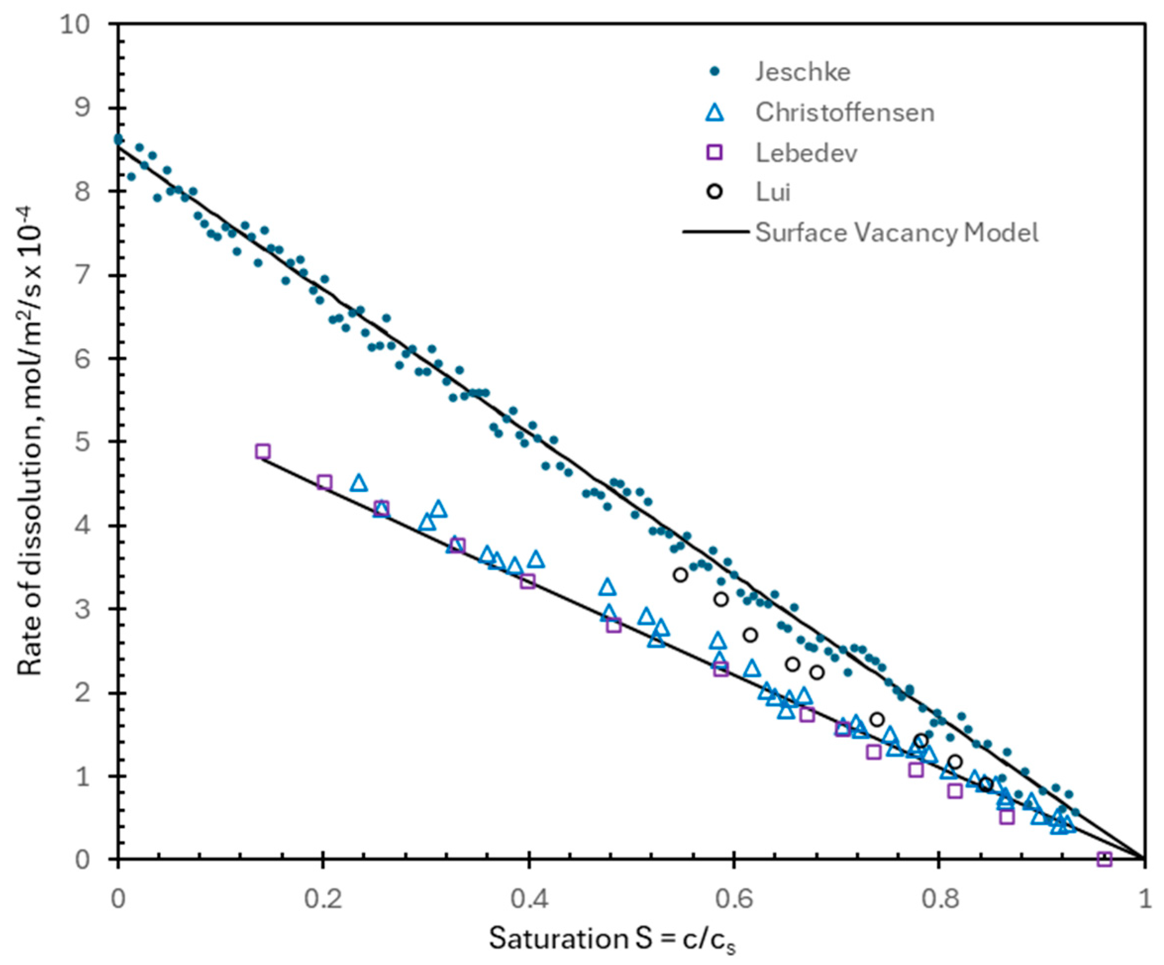
The dissolution of gypsum, CaSO₄·2H₂O, has been studied repeatedly [3]. The experimental results are shown in Figure 5, where it is clear that the rate of dissolution is a linear function of saturation. Colombani [3] examined the impact of diffusional processes on the rate of dissolution of gypsum, and those studies that were unduly influenced by diffusion were not included in Figure 5 [27]. These results are described by Equation (29) as shown in the line in Figure 5.

Figure 5. The rate of dissolution of gypsum in purified water as a function of saturation from different authors at either 20 °C or 25 °C. Differences between authors are due to different natural samples used. Data from different studies were collated and assessed by Colombani [3]. The equilibrium concentration of calcium in solution is 15.3 × 10⁻³ mol/L [3].

3.2. Non-Linear Kinetics, Saturation Order Greater than One

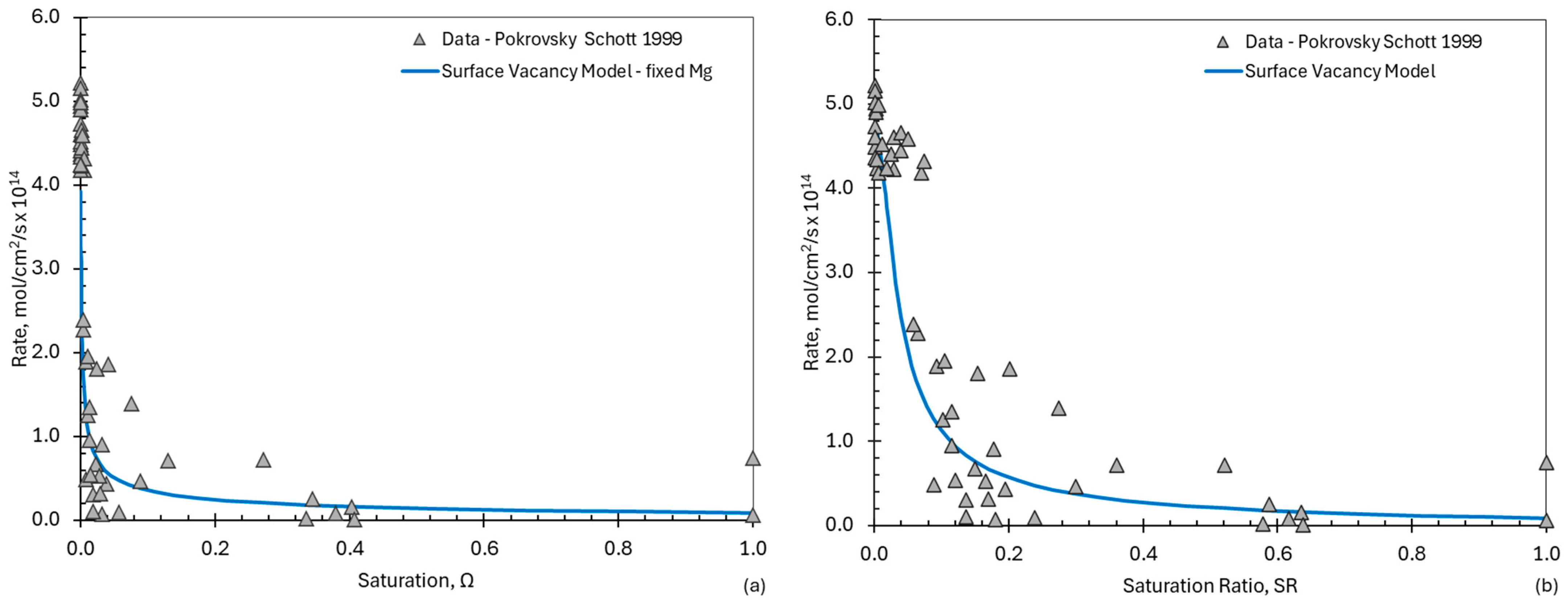
Generally, the dissolution of sparingly soluble salts has been reported as non-linear, that is, the ‘saturation order’ n is greater than one. An example of such a non-linear case is that of magnesite. The dissolution of magnesite, MgCO₃, in alkaline solutions at 25 °C was studied by Pokrovsky and Schott [44], who presented data on the rate as a function of the concentration of Mg²⁺ in solution and the chemical affinity. This data can be transformed into a rate as a function of Mg²⁺ and CO₃²⁻ in solution. The rate of dissolution of magnesite is dependent on pH below pH 5, whereas above this value, it is not directly influenced. Because we wish to test this model without the additional factor pH, data above pH 5 was selected from their dataset.

The data for the rate of dissolution in solution as a function of the saturation state, Ω, is given in Figure 6. To confirm that the non-linearity of the data for magnesite is not an artifact of using the saturation state as the independent variable instead of the saturation, S, the data was also plotted as a function of the saturation ratio, SR, where the saturation ratio is defined as $SR={\left({c_{+}}^m{c_{-}}^a/K_{sp}\right)}^{1/m+a}={\left(c_{+}{c}_{-}/K_{sp}\right)}^{1/2}$ [6]. SR can be interpreted as a mean concentration. These results are also shown in Figure 6 and demonstrate that the dissolution of magnesite is non-linear with respect to both Ω and SR.

Figure 6. The rate of dissolution of magnesite as a function of (a) saturation, Ω, and (b) saturation ratio (SR) at 25 °C and ionic strength greater than or equal to 0.01 M. The data of Pokrovsky and Schott [44] is shown as the points. The line represents the surface vacancy model with 0.001 mM Mg²⁺.

Application of Equation (22) to the case of the dissolution of magnesite in alkaline solutions yields Equation (30).

$$\overrightarrow{r}={\displaystyle \frac{k_1\left(1-[M{g}^{2+}][C{O}_3^{2-}]/K_{sp}\right)}{{\left(1+k_2[M{g}^{2+}]\right)}^{\raisebox{1ex}{$1$}\!\left/ \!\raisebox{-1ex}{$2$}\right.}{\left(1+[C{O}_3^{2-}]/K_{sp}{k}_2\right)}^{\raisebox{1ex}{$1$}\!\left/ \!\raisebox{-1ex}{$2$}\right.}}}$$

(30)

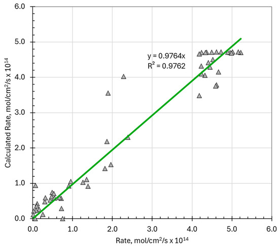
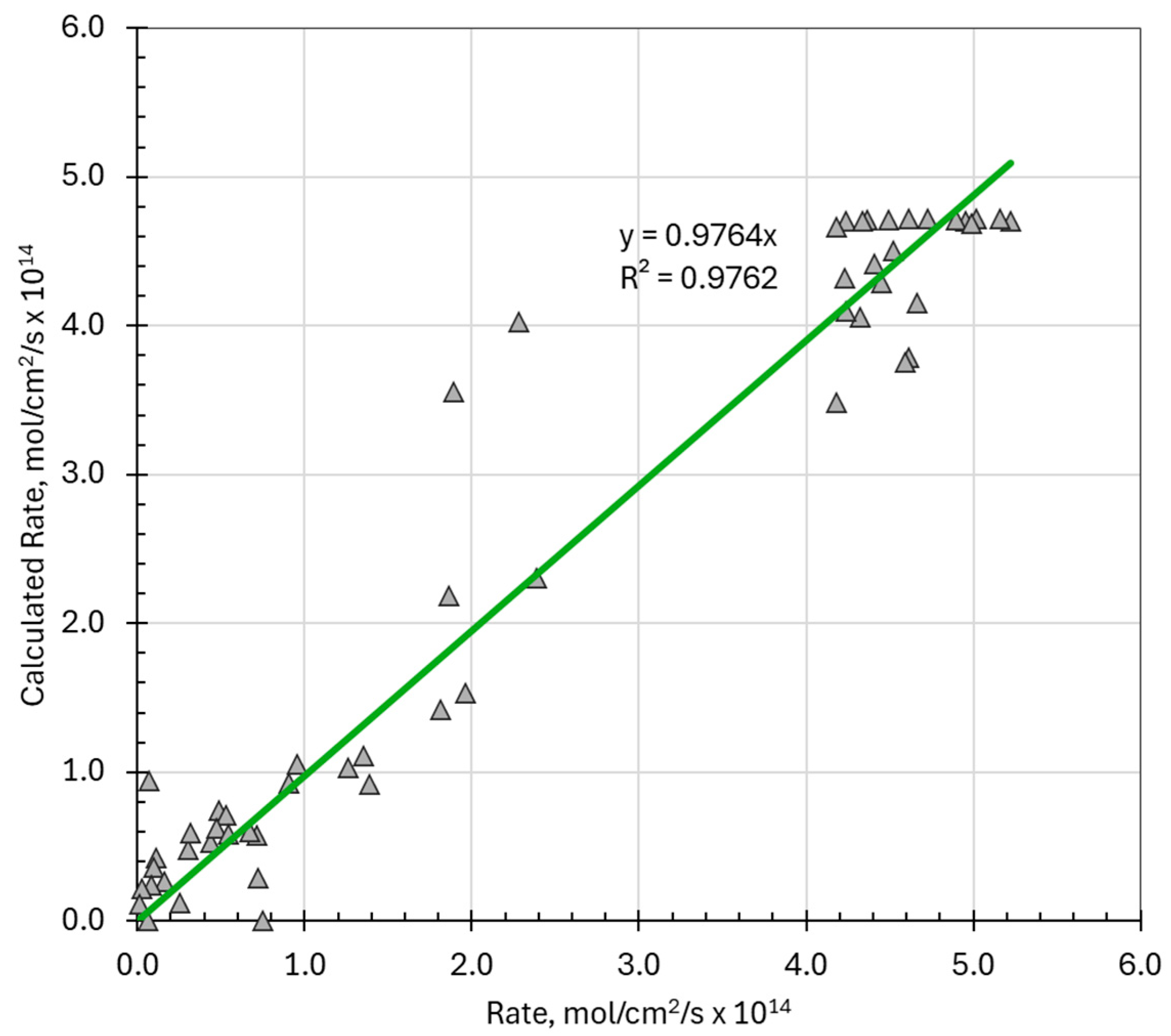
The values of $k_1$ and $k_2$ were estimated by non-linear least-squares regression [45], which yielded values of 4.72 mol/cm²/s and 134 M⁻¹, respectively. The calculated values of the rate using Equation (30) against the measured rate of dissolution are shown in Figure 7. The regression of the calculated and measured rates has a slope of 0.97, close to the expected slope of 1.0, with an R² of 0.97 with 56 degrees of freedom, indicating that Equation (30) is a good description of the data.

Figure 7. The correspondence between the calculated rate of dissolution and the corresponding measured rate of dissolution. The points represent data, and the line represents a regression of calculated with data for which the slope should be 1.0.

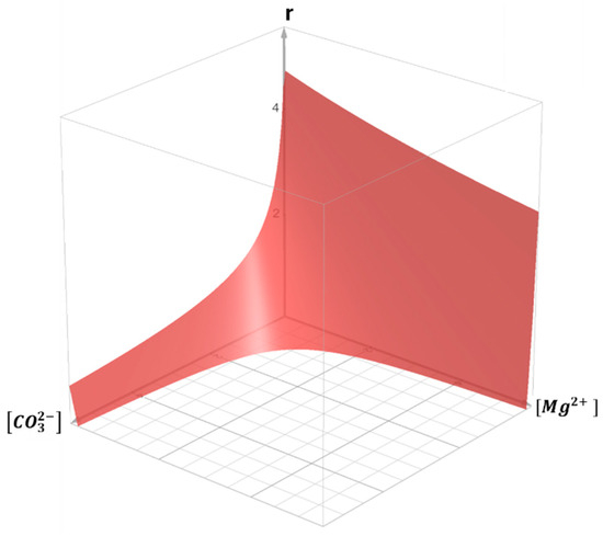
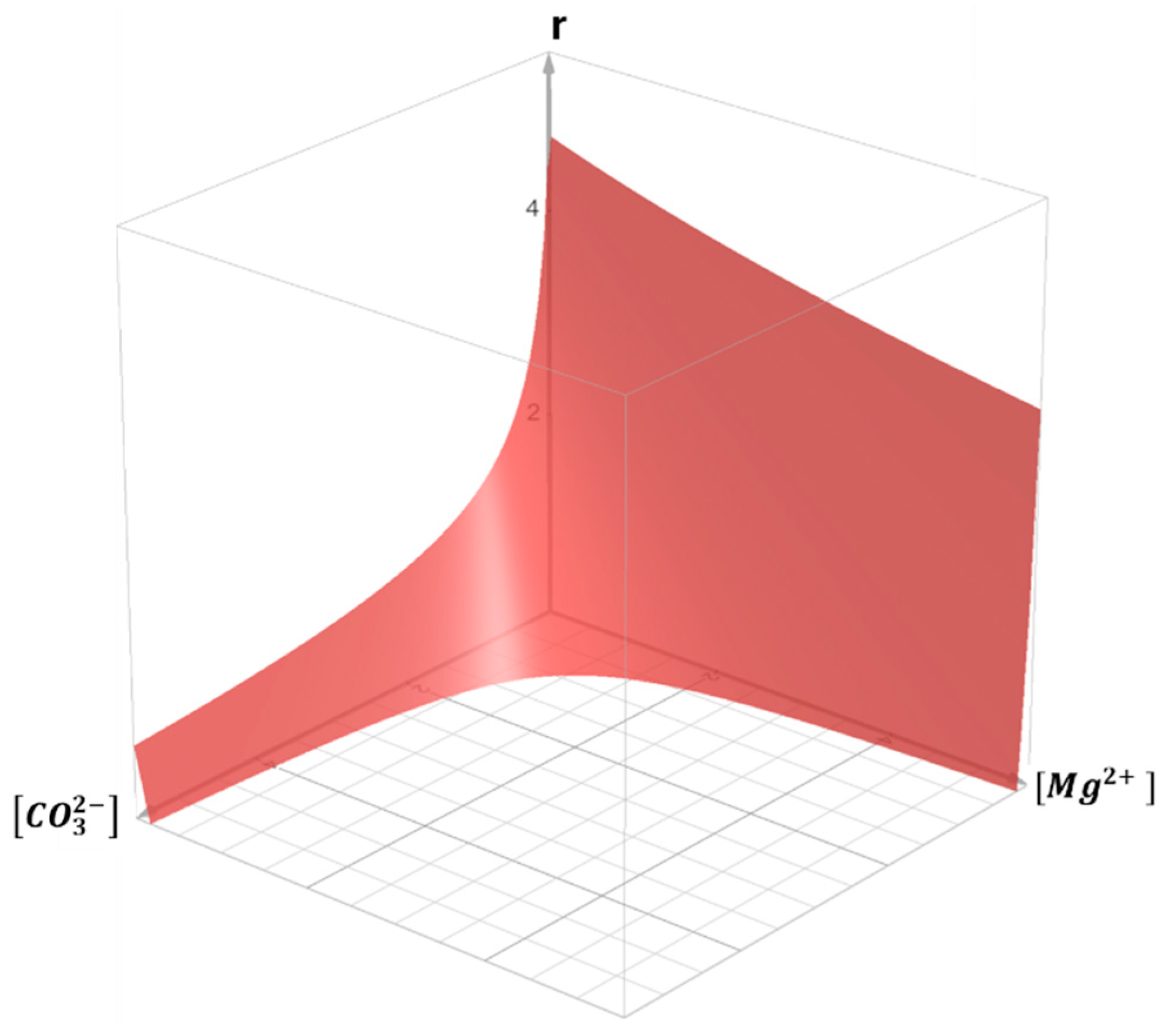
A three-dimensional plot of Equation (30) with the fitted parameters is shown in Figure 8. On the plane represented by equilibrium conditions, that is, when r = 0, changes in the concentrations of ${Mg}^{2+}$ and ${CO}_3^{2-}$ ions are described by a symmetrical hyperbola, as expected from the equilibrium condition. However, as the rate increases, an asymmetry appears, as can be seen from the shape of the curves at the planes representing the walls of Figure 8. The rate of dissolution in this region is more sensitive to the concentration of ${CO}_3^{2-}$ than to the concentrations of ${Mg}^{2+}$ by an order of magnitude. This asymmetry has not been previously recognized.

Figure 8. The 3-D surface of the rate of dissolution, calculated from Equation (30), as a function of the concentrations of ${CO}_3^{2-}$ and ${Mg}^{2+}$ ions in solution.

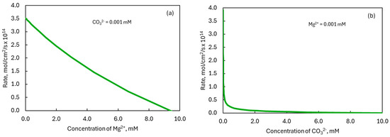
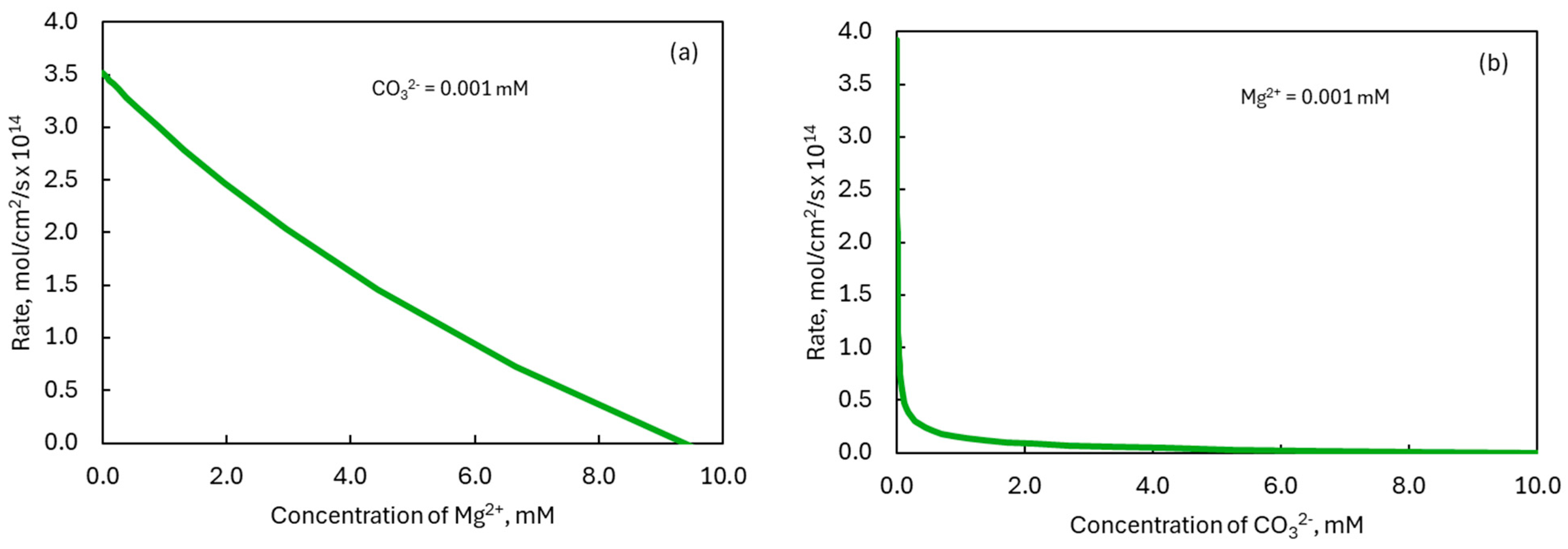
The projection of the 3-D surface onto each of the planes for which the concentration is 0.001 mM is shown in Figure 9, which emphasizes different functional dependencies of the rate on the concentration of ${CO}_3^{2-}$ compared to that on the concentration of ${Mg}^{2+}$. Experimental studies in dissolution kinetics endeavor to vary only one factor while holding all others constant. Figure 8 and Figure 9 indicate how holding the concentration of ${CO}_3^{2-}$ constant and investigating the effect of the concentration of ${Mg}^{2+}$ on the rate might lead to very different conclusions to those that might have been reached if the opposite experimental strategy had been adopted. The experimental program needs to measure and adjust the concentrations of both constituent ions to fully understand the kinetics of dissolution.

Figure 9. The rate of dissolution of magnesite as a function of the concentrations of (a) ${Mg}^{2+}$ ions in solution at a constant concentration of ${CO}_3^{2-}$ ions of 0.001 mM and (b) ${CO}_3^{2-}$ ions in a solution of ${Mg}^{2+}$ ions of 0.001 mM.

3.3. Surface Charge and Potential

Ibl et al. [18] showed that the potential across the crystal membrane is directly influenced by the processes of dissolution and crystallization. Linge [20] suggested that this might be the key to the understanding of dissolution and crystallization. The surface vacancy model for sparingly soluble salts follows this path. It is based on the formation of surface charge due to ‘self-ionization’ and the impact that this surface charge has on the rate of removal of anions and cations from the surface. Electrochemistry is an inherent part of the model.

The interfacial potential difference, given by Equation (19) for stoichiometric dissolution at the stationary state (when $d{\sigma }_0/dt$ is zero) is expressed in terms of the parameter $k_2$ and the solubility product in Equation (31).

$$\Delta \varphi ={\displaystyle \frac{RT}{F}}\ln \left({\displaystyle \frac{{\overrightarrow{k}}_{+}}{{\overrightarrow{k}}_{-}}}\right)+{\displaystyle \frac{RT}{F}}\ln \left({\displaystyle \frac{1+k_2{c}_{+}}{1+c_{-}/k_2{K}_{sp}}}\right)$$

(31)

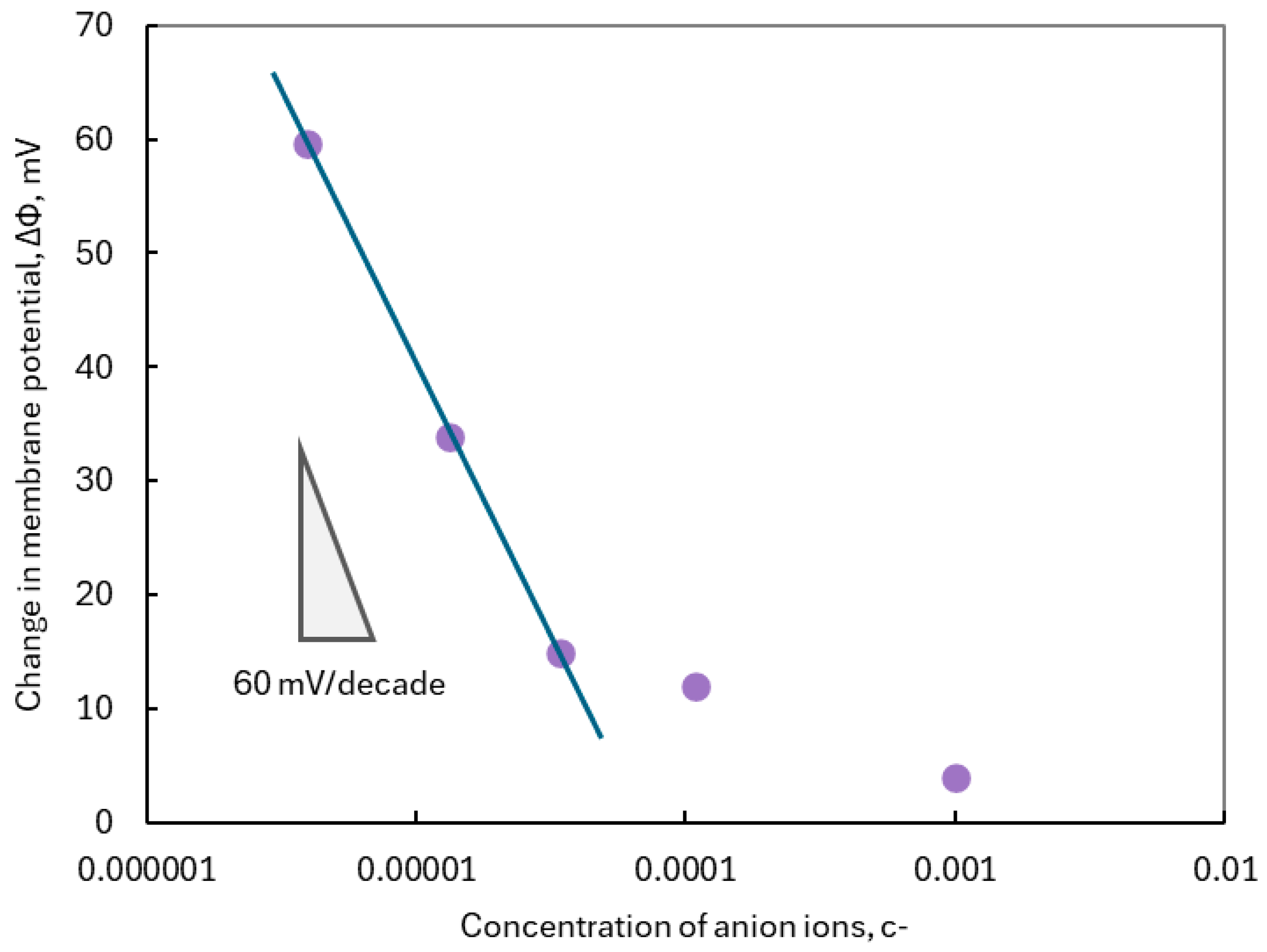
Equation (31) indicates that if the dissolution is linear in concentration, that is, it follows Equation (29), then the effect of anions and cations on the interfacial potential difference will be symmetrical or close to symmetrical. Under these conditions, the slope of the plot of $\Delta \varphi$ against the base 10 logarithm of the concentration will be about −60 mV/decade ($-2.303RT/F$).

On the other hand, for low concentrations of anions and cations, the interfacial potential difference will be independent of concentration. More specifically, if either of the conditions $c_{-}{\overleftarrow{k}}_{-}/{\overrightarrow{k}}_{+}\ll 1$ or $c_{+}{\overleftarrow{k}}_{+}/{\overrightarrow{k}}_{-}\ll 1$ are met, then Equations (19) and (31) are independent of the concentration of the anion or cation.

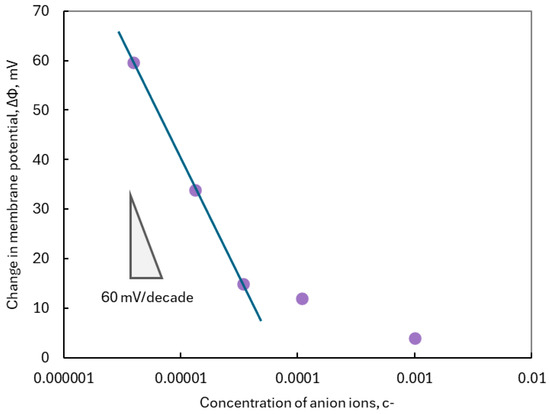
The results reported by Jaenicke [19] for the effect of the concentration of the anion on the interfacial potential difference are plotted in Figure 10. Interestingly, the slope of the data at the lower concentrations has a slope close to −60 mV/decade, in agreement with Equation (31). The deviation at higher concentrations of the anion might be due to the influence of mass transfer, but this requires further investigation.

Figure 10. The effect of the concentration of anion on the interfacial potential difference for AgCl. Data from Jaenicke [19] shown as points.

The slope of the data of Tani et al. [17] shown in Figure 1 is also close to −60 mV/decade. Since the rate constant for the removal of cations, ${\overrightarrow{k}}_{+}$ is small; there is no limiting region suggested by the non-Nernstian form of Equations (19) and (31). For this reason, the membrane potential is affected by the concentration of fluoride ions even at low levels.

A feature of the proposed model is the region where the potential is no longer dependent on the concentration of the constituent ion when the concentration of that ion is sufficiently low. Only a limited number of studies of the membrane potentials of sparingly soluble salts have been made. However, it is more common to measure the zeta potential of these salts. The zeta potential is the potential difference between the point of hydrodynamic shear and the bulk solution. Because both the interfacial potential difference (over the Helmholtz layer) and the zeta potential are both dependent on the charge developed at the surface, they are related to one another [36]. There is evidence from zeta potential measurements of a limiting region where, below a certain concentration of the potential-determining ion, the zeta potential is constant [35]. This limiting region has been interpreted in terms of the formation of an adsorption layer [46]. While a chemically distinct adsorption layer of constituent ions is difficult to accept, the application of Equation (19) to interpret the results of zeta potential experiments should be revisited in more detail than is possible here.

3.4. Non-Stoichiometric Dissolution

The mechanism of dissolution proposed here has the advantage over all other models of dissolution of being able to describe non-stoichiometric dissolution if the assumption of dissolution at the stationary state is relaxed. (This assumption was made to derive Equation (15) from Equation (14)). However, returning the analysis to Equation (14) requires knowledge of the initial value of the interfacial potential difference, which is not available in normal dissolution experiments. There are, however, two possibilities: (i) the initial potential difference is greater than the potential difference at stoichiometric dissolution, or (ii) it is less than the stoichiometric value. Dissolution behavior for both possibilities leads to different non-stoichiometric behavior.

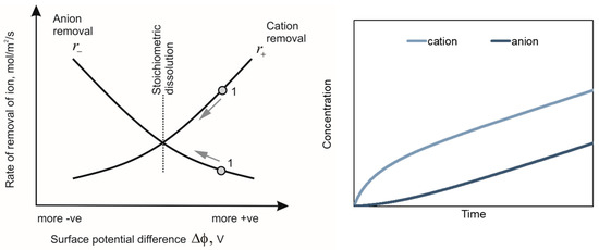
The first case is illustrated graphically in Figure 11. The curves for the rates of removal of anions and cations as a function of potential are shown in the left-hand frame. The condition for stoichiometric dissolution occurs where these two curves intersect. If the sparingly soluble salt has a potential difference that is initially higher than the stoichiometric value, at point 1, for example, the rate of dissolution of the cation is initially faster than that of the anion, since $r_{+}$ is greater than $r_{-}$ at the potential of point 1. As dissolution proceeds, these unequal rates of dissolution will move the interfacial potential difference towards the stoichiometric value. Once this stoichiometric point is reached, the rates of removal of the anions and cations become equal, and dissolution becomes stoichiometric.

Figure 11. The explanation for non-stoichiometric dissolution. If the initial surface potential is at point 1 on immersion, the rate of dissolution of cations will be greater than that of anions. The direction with time of the reaction from the initial condition is shown by the arrows.

The concentration profiles with time for this possibility are shown in the panel on the right-hand side of Figure 11. Initially, the rate of removal of the cations is faster than that of the anion. As dissolution proceeds, the rate of removal of the cation slows, and the anions accelerate to the point where they are equal, that is, their slopes are equal. Such behavior is frequently observed for dissolution reactions—there is an initial surge, and then the rate becomes steady.

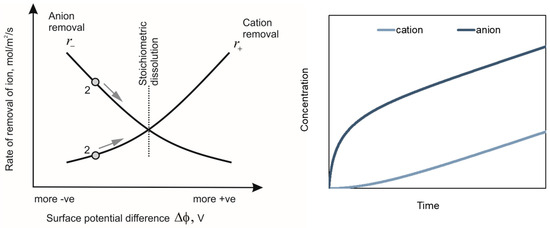
The second case occurs when the initial value of the interfacial potential difference is below that at which stoichiometric dissolution occurs. In this case, illustrated at point 2 in Figure 12, the rate of removal of the anion, $r_{-}$, exceeds the rate of removal of the cation, $r_{+}$. Again, with continued dissolution, the unequal rates of removal of anions and cations will move the potential difference towards the value for stoichiometric dissolution.

Figure 12. The explanation for non-stoichiometric dissolution. If the initial surface potential is at point 2 on immersion, the rate of dissolution of anions will be greater than that of cations. The direction with time of the reaction from the initial condition is shown by the arrows.

Thus, the surface vacancy model explains non-stoichiometric dissolution. It is the only model of dissolution that has an explanation for non-stoichiometric dissolution.

Non-stoichiometric dissolution is a transient effect that also has implications for the experimental determination of the rates of dissolution. The observation of transient dissolution kinetics has been used to justify the proposal that a product layer forms on the surface, referred to as a ‘leach layer’ or that there is an adsorbed layer of constituent ions [38]. However, this may not necessarily be the case. On the other hand, an ‘induction period’ is sometimes observed. Depending on the state of the surface and the ion (cation or anion) that is measured to determine the rate, either an initial surge or an induction period might be observed. The mechanism proposed here explains how this might arise.

4. Conclusions

In this paper, the mechanism proposed by Crundwell [26,27] has been shown to provide a consistent explanation for (i) the linear and non-linear kinetics with respect to the saturation and the saturation state, (ii) the formation of a surface charge and potential difference, and (iii) non-stoichiometric dissolution. The model is based on the independent electrochemical removal of anions and cations from the surface, creating surface vacancies that carry charge. This surface charge results in a potential difference across the interface, which influences the rate of the electrochemical removal of the ions.

The rate equation derived from this model describes both linear and highly non-linear kinetics observed for sparingly soluble salts. Linear kinetics arise when the rate constants for anions and the cations exhibit symmetry, while non-linear kinetics arise when there is no such symmetry. Examples of gypsum (linear) and magnesite (non-linear) were used to illustrate the ability of the model to describe these situations.

Because the model is electrochemical in nature, it coherently describes the development of the interfacial potential difference as an inherent part of the model. While not many direct measurements of the interfacial potential difference have been made for sparingly soluble salts, the model is consistent with those that are available.

The model is unique in that it is the only mechanism of dissolution that has been proposed that is able to describe non-stoichiometric dissolution.

Further experimental work is required in which dissolution rates, membrane potentials, and non-stoichiometric dissolution are observed under the same conditions.

References

- Crundwell, F.K. The mechanism of dissolution of minerals in acidic and alkaline solutions: Part I—A new theory of non-oxidation dissolution. Hydrometallurgy 2014, 149, 252–264. [Google Scholar] [CrossRef] [Scilit]
- Liu, S.; Nancollas, G. The kinetics of dissolution of calcium sulfate dihydrate. J. Inorg. Nucl. Chem. 1971, 33, 2311–2316. [Google Scholar] [CrossRef] [Scilit]
- Colombani, J. Measurement of the pure dissolution rate constant of a mineral in water. Geochim. Cosmochim. Acta 2008, 72, 5634–5640. [Google Scholar] [CrossRef] [Scilit]
- Davies, C.W.; Nancollas, G.H. The precipitation of silver chloride from aqueous solutions. Part 3. Trans. Faraday Soc. 1955, 51, 818–823. [Google Scholar] [CrossRef] [Scilit]
- Konak, A.R. Surface reaction-controlled dissolution of crystals in a solvent or solution. Chem. Eng. Sci. 1974, 29, 1785–1788. [Google Scholar] [CrossRef] [Scilit]
- Zhang, J.-W.; Nancollas, G.H. Mechanisms of growth and dissolution of sparingly soluble salts. Rev. Mineral. Geochem. 1990, 23, 365–396. [Google Scholar]
- Bovington, C.H.; Jones, A.L. Tracer study of the kinetics of dissolution of lead sulphate. Trans. Faraday Soc. 1970, 66, 2088–2091. [Google Scholar] [CrossRef] [Scilit]
- Bovington, C.H.; Jones, A.L. Tracer Study of the Kinetics of Dissolution of Barium Sulphate. Trans. Faraday Soc. 1970, 66, 764. [Google Scholar] [CrossRef] [Scilit]
- Campbell, J.R.; Nancollas, G.H. The crystallization and dissolution of strontium sulfate in aqueous solution. J. Phys. Chem. 1969, 73, 1735–1740. [Google Scholar] [CrossRef] [Scilit]
- Jones, A.L.; Linge, H.G.; Wilson, I.R. The dissolution of silver chromate into aqueous solutions. J. Crystal Growth 1975, 28, 254–258. [Google Scholar] [CrossRef] [Scilit]
- Jones, A.L.; Madigan, G.A.; Wilson, I.R. The dissolution and growth of barium iodate crystals. J. Crystal Growth 1973, 20, 93–98. [Google Scholar] [CrossRef] [Scilit]
- Hamza, S.M.; Abdul-Rahman, A.; Nancollas, G.H. The influence of magnesium ion on the kinetics of crystal growth and dissolution of strontium fluoride. J. Crystal Growth 1985, 73, 245–250. [Google Scholar] [CrossRef] [Scilit]
- Gardner, G.L.; Nancollas, G.H. Kinetics of crystal growth and dissolution of calcium and magnesium fluorides. J. Dent. Res. 1976, 55, 342–352. [Google Scholar] [CrossRef] [Scilit]
- Christoffersen, J.; Christoffersen, M.R.; Kibalczyc, W.; Perdok, W.G. Kinetics of dissolution and growth of calcium fluoride and effects of phosphate. Acta Odontol. Scand. 1988, 46, 325–336. [Google Scholar] [CrossRef] [Scilit]
- Romanek, C.S.; Morse, J.W.; Grossman, E.L. Aragonite kinetics in dilute solutions. Aquat. Geochem. 2011, 17, 339–356. [Google Scholar] [CrossRef] [Scilit]
- Ruiz-Agudo, E.; Putnis, C.V.; Rodriguez-Navarro, C.; Putnis, A. Mechanism of leached layer formation during chemical weathering of silicate minerals. Geology 2012, 40, 947–950. [Google Scholar] [CrossRef] [Scilit]
- Tani, Y.; Umezawa, Y.; Chikama, K.; Hemmi, A.; Soma, M. Non- stoichiometric dissolution of lanthanum fluoride (LaF3) and its relevance to a process of ion-selective charge separation at the solid solution interface. J. Electroanal. Chem. 1994, 378, 205–213. [Google Scholar] [CrossRef] [Scilit]
- Ibl, N.; Richardz, W.; Wiederkehr, H. The connection between electric potential and crystallization. Z. Phys. Chem. 1975, 98, 123–142. [Google Scholar] [CrossRef] [Scilit]
- Jaenicke, W. Uber den Zusammenhang zwischen Potential und Auf losungsgeschwindigkeit von Salzen. Z. Elektrochem. 1952, 52, 473–476. [Google Scholar]
- Linge, H.G. Dissolution of ionic crystal surfaces. Adv. Colloid Interface Sci. 1981, 14, 239–250. [Google Scholar] [CrossRef] [Scilit]
- Nielsen, A.R. Electrolyte crystal growth mechanisms. J. Crystal Growth 1984, 67, 289–310. [Google Scholar] [CrossRef] [Scilit]
- Davies, C.W.; Jones, A.L. The precipitation of silver chloride from aqueous solutions. Part 2. Trans. Faraday Soc. 1955, 51, 812–817. [Google Scholar] [CrossRef] [Scilit]
- Jones, A.L.; Linge, H.G. Inadequacy of Theories for Crystal Dissolution. Z. Phys. Chem. 1975, 95, 293–296. [Google Scholar] [CrossRef] [Scilit]
- Konak, A.K. Difficulties associated with theories of growth from solutions. J. Crystal Growth 1973, 19, 247–252. [Google Scholar] [CrossRef] [Scilit]
- Vermilyea, D.A. The dissolution of ionic compounds in aqueous media. J. Electrochem. Soc. 1966, 113, 1067–1070. [Google Scholar]
- Crundwell, F.K. The impact of surface charge on the ionic dissociation of common salt (NaCl). Chem. Eng. Sci. 2019, 205, 174–180. [Google Scholar] [CrossRef] [Scilit]
- Crundwell, F.K. On the mechanism of the dissolution of gypsum (calcium sulfate dihydrate). Hydrometallurgy 2025, 236, 106535. [Google Scholar] [CrossRef] [Scilit]
- Crundwell, F.K. The mechanism of dissolution of minerals in acidic and alkaline solutions: Part II Application of a new theory to silicates, aluminosilicates and quartz. Hydrometallurgy 2014, 149, 265–275. [Google Scholar] [CrossRef] [Scilit]
- Crundwell, F.K. The mechanism of dissolution of minerals in acidic and alkaline solutions: Part III. Application to oxide, hydroxide and sulfide minerals. Hydrometallurgy 2014, 149, 71–81. [Google Scholar] [CrossRef] [Scilit]
- Crundwell, F.K. The mechanism of dissolution of minerals in acidic and alkaline solutions: Part IV—Equilibrium and near equilibrium behaviour. Hydrometallurgy 2015, 153, 46–57. [Google Scholar] [CrossRef] [Scilit]
- Crundwell, F.K. The mechanism of dissolution of minerals in acidic and alkaline solutions: Part V—Surface charge and zeta potential. Hydrometallurgy 2016, 162, 174–184. [Google Scholar] [CrossRef] [Scilit]
- Crundwell, F.K. The mechanism of dissolution of minerals in acidic and alkaline solutions: Part VI—A molecular viewpoint. Hydrometallurgy 2016, 161, 34–44. [Google Scholar] [CrossRef] [Scilit]
- Crundwell, F.K. The surface vacancy model—A general theory of the dissolution of salts and minerals. Minerals 2021, 11, 521. [Google Scholar] [CrossRef] [Scilit]
- Grimley, T.B. The Contact between a Solid and an Electrolyte. Roy. Soc. Proc. A 1950, 201, 40–61. [Google Scholar] [CrossRef] [Scilit]
- Hunter, R.J. Zeta Potential in Colloid Science; Academic Press: New York, NY, USA, 1981. [Google Scholar]
- Crundwell, F.K. On the mechanism of the flotation of oxides and silicates. Miner. Eng. 2016, 104, 185–196. [Google Scholar] [CrossRef] [Scilit]
- Velbel, M.A. Bond strength and relative weathering rate of simple orthosilicates. Am. J. Sci. 1999, 299, 679–696. [Google Scholar] [CrossRef] [Scilit]
- Aagaard, P.; Helgeson, H.C. Thermodynamic and kinetic constraints on reaction rates among minerals and aqueous solutions. I Theoretical considerations. Am. J. Sci. 1982, 282, 237–285. [Google Scholar]
- Bard, A.J.; Faulkner, L.R. Electrochemical Methods: Fundamentals and Applications; John Wiley and Sons: New York, NY, USA, 1980. [Google Scholar]
- Vetter, K.J. Electrochemical Kinetics—Theoretical Aspects; Academic Press: New York, NY, USA, 1967. [Google Scholar]
- Lyklema, J. Electrified interfaces in aqueous dispersions of solids. Pure Appl. Chem. 1991, 63, 895–906. [Google Scholar] [CrossRef] [Scilit]
- Lyklema, J. Surface charges and electrokinetic charges—Distinctions and juxtapositionings. Colloids Surf. A Physicochem. Eng. Asp. 2011, 376, 2–8. [Google Scholar] [CrossRef] [Scilit]
- Simon, B. Dissolution rates of NaCl and KCI in aqueous solution. J. Crystal Growth 1981, 52, 789–794. [Google Scholar] [CrossRef] [Scilit]
- Pokrovsky, O.S.; Schott, J. Processes at the magnesium-bearing carbonates/solution interface. II. Kinetics and mechanism of magnesite dissolution. Geochim. Cosmochim. Acta 1999, 63, 881–897. [Google Scholar] [CrossRef] [Scilit]
- Press, W.H.; Teukolsky, S.A.; Vetterling, W.T.; Flannery, B.P. Numerical Recipes: The Art of Scientific Computing; Cambridge University Press: Cambridge, UK, 2007. [Google Scholar]
- LuValle, J.E.; Jackson, J.M. The zeta potential of silver bromide in the presence of various substances of photographic interest. J. Phys. Chem. 1953, 61, 1216–1222. [Google Scholar] [CrossRef] [Scilit]
Disclaimer/Publisher’s Note: The statements, opinions and data contained in all publications are solely those of the individual author(s) and contributor(s) and not of MDPI and/or the editor(s). MDPI and/or the editor(s) disclaim responsibility for any injury to people or property resulting from any ideas, methods, instructions or products referred to in the content. |
© 2026 by the author. Licensee MDPI, Basel, Switzerland. This article is an open access article distributed under the terms and conditions of the Creative Commons Attribution (CC BY) license.