Likelihood and Bayesian Inference for Two Lomax Populations Under Balanced Joint Adaptive Progressive Type-II Censoring with an Exponential Ridge

Abstract

Balanced joint adaptive progressive Type-II censoring (B-JAPC) is developed for two independent Lomax populations with a common shape parameter and population-specific scale parameters. Classical and Bayesian inference methods are constructed for the model parameters, survival functions, and hazard rates. To address the exponential scale–shape ridge where standard maximum likelihood estimates often fail to converge, a constrained maximum likelihood estimator (CMLE) with parametric bootstrap confidence intervals is established. A partially conjugate Bayesian framework under a Beta–Gamma prior is also implemented via a Metropolis-within-Gibbs algorithm. Monte Carlo simulations demonstrate that the proposed adaptive design substantially reduces the mean test duration compared to non-adaptive schemes while maintaining high inferential accuracy. The methodology is successfully applied to randomized cloud-seeding rainfall data, confirming its practical utility and quantifying the sensitivity of lifetime inference to shape regularization.

1. Introduction

Lifetime studies in reliability engineering, survival analysis, and industrial quality control rarely observe every lifetime completely. Test units may be expensive, intact units may be needed for other experiments, and a study may be required to deliver a prescribed number of failures within a practically acceptable period. Progressive Type-II censoring addresses these constraints by fixing the number of observed failures in advance while allowing surviving units to be withdrawn at successive failure times. It thereby generalizes ordinary Type-II censoring and permits the experimental cost, duration, and information content to be balanced through the withdrawal plan; systematic treatments are given by Balakrishnan and Aggarwala [1] and Balakrishnan and Cramer [2].

The design problem becomes more delicate in a comparative lifetime experiment, where units from two production lines or treatments are tested simultaneously and inference concerns their relative reliability. Rasouli and Balakrishnan [3] developed joint progressive Type-II censoring for two populations. In that construction, the numbers withdrawn from the two risk sets can depend strongly on the population in which the current failure occurs, which can produce unbalanced risk sets and analytically complicated likelihoods. Mondal and Kundu [4] proposed a balanced two-sample progressive scheme that equalizes the total reduction of the two risk sets at each planned withdrawal time. Subsequent work extended the balanced design from exponential populations to Weibull models and developed Bayesian and optimal-design procedures [5,6].

A fixed progressive withdrawal plan does not, however, control the realized duration of a study. The adaptive Type-II design of Ng et al. [7] modifies future withdrawals after a prespecified time while preserving the target number of failures. For two samples, Sultana et al. [8] introduced a joint adaptive progressive censoring scheme for exponential populations, and Sultana et al. [9] developed likelihood and Bayesian inference for Weibull populations. The prespecified time acts as a tuning threshold: after it is exceeded, intermediate withdrawals are suppressed, leaving more units at risk for the remaining failures. The threshold is not a deterministic upper bound on the terminal failure time.

The Lomax distribution, also known as the Pareto Type-II distribution, was introduced in the analysis of business-failure data by Lomax [10]. Its polynomially decaying survival function and decreasing hazard rate make it a natural alternative to the exponential distribution for heterogeneous populations, complex wear-in phase engineering systems, software debugging, and heavy-tailed lifetime data. Beyond its empirical versatility, the Lomax distribution exhibits a fundamental threshold stability property: conditional on survival past a time t, the remaining lifetime $X-t\mid X>t$ remains Lomax-distributed with the same shape parameter $\alpha$ and a shifted scale parameter $\lambda +t$. This property aligns naturally with adaptive progressive censoring designs, where risk sets are re-evaluated and intermediate withdrawals are modified dynamically after a prespecified threshold time $\tau$.

In two-sample comparative lifetime studies, assuming a common shape parameter $\alpha$ alongside population-specific scale parameters $({\lambda }_1,{\lambda }_2)$ is both mathematically convenient and scientifically justified. Physically, a shared shape parameter indicates that units from both populations undergo identical underlying failure mechanisms or aging physics (e.g., electronic components produced via similar manufacturing processes or mechanical parts subject to similar stress regimes), whereas distinct scale parameters capture variations in baseline endurance, material quality, or operational environments. In survival analysis, this formulation also directly corresponds to a proportional hazard or accelerated life framework. Furthermore, early-stage failure processes—such as burn-in testing of electronic components, initial mechanical running-in, or mortality early after intervention—naturally exhibit decreasing hazard rates, where units that survive initial stresses become progressively more reliable over time.

Motivated by these theoretical and applied advantages, the present study considers two Lomax populations under balanced joint adaptive progressive Type-II censoring (B-JAPC). The principal contributions are as follows:

(1)

Methodological Framework: The B-JAPC design is formulated to unify balanced joint progressive censoring and pooled joint Type-II censoring, establishing its risk-set balancing identity and leveraging the threshold stability of the Lomax distribution for missing-data imputation.

(2)

Analytical and Numerical Profiling: Likelihood equations and score vectors are derived for the common-shape two-sample Lomax model. The nonregular exponential scale–shape ridge is formally characterized, and a constrained maximum likelihood estimator (CMLE) is proposed with sensitivity analyses to ensure regular identifiability.

(3)

Bayesian and Reliability Inference: A partially conjugate Beta–Gamma Bayesian analysis is constructed alongside an order-restricted MCMC algorithm, delivering robust point and interval estimates for both parameters and key reliability metrics ($S(t)$ and $h(t)$).

(4)

Empirical Quantification: Extensive Monte Carlo simulations quantify the substantial reduction in test duration achieved by B-JAPC (up to $62.6\%$), and a real-data cloud-seeding application demonstrates its practical utility.

For clarity, the abbreviations used throughout the manuscript are summarized in Abbreviations. The remainder is organized as follows. Section 2 describes the censoring scheme and Lomax model, Section 3 presents likelihood-based inference, and Section 4 gives Bayesian estimation. Simulation and real-data analyses are combined in Section 5, followed by conclusions in Section 6. Detailed proofs, derivatives, and algorithms are placed in Appendix A, Appendix B, Appendix C and Appendix D.

2. Model Description

2.1. Balanced Joint Adaptive Progressive Type-II Censoring

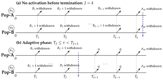
Place $n_1$ units from population 1 (Pop-A) and $n_2$ units from population 2 (Pop-B) on test. Fix a target of k observed failures, a tuning time $\tau >0$, and non-negative planned withdrawals $R_1,\dots ,R_{k-1}$ satisfying ${\sum }_{i=1}^{k-1}{R}_i\le \min (n_1,n_2)-k$. Let $0<T_1<\cdots <T_k$ denote the ordered observed failure times and let $M_i=1$ if the failure at $T_i$ comes from Pop-A and $M_i=0$ otherwise. With $T_0=0$, define

$$J=\max \{j\in \{0,1,\dots ,k\}:T_j\le \tau \}.$$

(1)

When $\tau \ge T_k$, $J=k$ and all k failure times occur before the threshold. More generally, whenever $\tau \ge T_{k-1}$, all $k-1$ planned intermediate withdrawals $(R_1,\dots ,R_{k-1})$ are fully executed prior to $\tau$. Consequently, no adaptive suppression of withdrawals takes place, and the B-JAPC design collapses to the standard nonadaptive B-JPC scheme for any $\tau \ge T_{k-1}$ (where $J=k-1$ if $T_{k-1}\le \tau <T_k$, and $J=k$ if $\tau \ge T_k$).

For $i<k$, the actual withdrawals from Pop-A and Pop-B are

$$A_{1i}=\mathbb{I}(i\le J)(R_i+1-M_i),A_{2i}=\mathbb{I}(i\le J)(R_i+M_i).$$

(2)

At $T_k$, all remaining units are removed:

$$\begin{array}{cc}{A}_{1k}\hfill & =n_1-{\displaystyle {\sum }_{i=1}^{k-1}}(A_{1i}+M_i)-M_k,\hfill \\ A_{2k}\hfill & =n_2-{\displaystyle {\sum }_{i=1}^{k-1}}(A_{2i}+1-M_i)-(1-M_k).\hfill \end{array}$$

(3)

Thus, before $\tau$, each risk set loses exactly $R_i+1$ units after failure and withdrawal; after $\tau$, intermediate withdrawals are cancelled. The observed data are ${\mathcal{D}}_{\tau }=\{(T_i,M_i,A_{1i},A_{2i}):i=1,\dots ,k\}$.

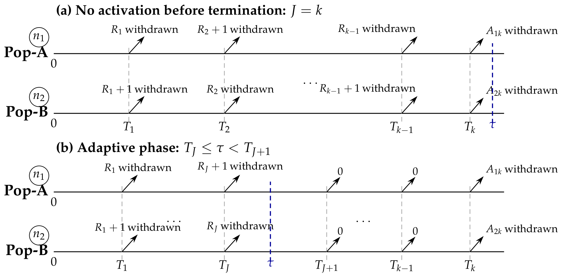
Figure 1 illustrates the nonadaptive and adaptive regimes. If $\tau \ge T_{k-1}$, the design reduces to B-JPC; if $\tau <T_1$, it reduces to pooled joint Type-II censoring. The threshold $\tau$ determines the withdrawal rule but does not impose an upper bound on $T_k$. The balancing proof and population-specific risk-set accounting are given in Appendix A.

Figure 1. B-JAPC censoring scheme. Panel (a) shows the nonadaptive B-JPC regime ($\tau \ge T_{k-1}$), where all intermediate withdrawals $R_1,\dots ,R_{k-1}$ are executed. Panel (b) shows the adaptive regime ($\tau <T_{k-1}$): balanced withdrawals are executed up to $T_J$, intermediate withdrawals are suppressed after $\tau$, and all remaining units are removed at $T_k$.

2.2. Two Lomax Populations

Assume

$$X\sim \mathrm{Lomax}({\lambda }_1,\alpha ),Y\sim \mathrm{Lomax}({\lambda }_2,\alpha ),$$

(4)

where ${\lambda }_1,{\lambda }_2>0$ are population-specific scale parameters and $\alpha >0$ is a common shape parameter. For $j=1,2$ and $t>0$,

$$\begin{array}{cccc}{f}_j(t)\hfill & ={\displaystyle \frac{\alpha }{{\lambda }_j}}{\left(1+{\displaystyle \frac{t}{{\lambda }_j}}\right)}^{-(\alpha +1)},\hfill & F_j(t)\hfill & =1-{\left(1+{\displaystyle \frac{t}{{\lambda }_j}}\right)}^{-\alpha },\hfill \\ S_j(t)\hfill & ={\left(1+{\displaystyle \frac{t}{{\lambda }_j}}\right)}^{-\alpha },\hfill & h_j(t)\hfill & ={\displaystyle \frac{\alpha }{{\lambda }_j+t}}.\hfill \end{array}$$

(5)

The hazard rate is decreasing. For common $\alpha$, ${\lambda }_1\le {\lambda }_2$ is equivalent to $S_1(t)\le S_2(t)$ and $h_1(t)\ge h_2(t)$ for every $t>0$; the result is established in Appendix A.

3. Likelihood-Based Inference

Let $d_{1i}=M_i$, $d_{2i}=1-M_i$, $C_{1i}=A_{1i}+M_i$, $C_{2i}=A_{2i}+1-M_i$, $K_j={\sum }_i{d}_{ji}$, $q_{ji}({\lambda }_j)=\log (1+T_i/{\lambda }_j)$, and 

$$Q({\lambda }_1,{\lambda }_2)={\displaystyle \sum _{i=1}^k}{C}_{1i}{q}_{1i}({\lambda }_1)+{\displaystyle \sum _{i=1}^k}{C}_{2i}{q}_{2i}({\lambda }_2).$$

Conditional on the realized censoring pattern, the likelihood is

$$L({\lambda }_1,{\lambda }_2,\alpha \mid {\mathcal{D}}_{\tau })\propto {\alpha }^k{\lambda }_1^{-K_1}{\lambda }_2^{-K_2}\exp \left\{-\sum _i{d}_{1i}{q}_{1i}-\sum _i{d}_{2i}{q}_{2i}-\alpha Q\right\}.$$

(6)

The score equations, observed information matrix, and delta-method derivatives are collected in Appendix A.

Remark 1 (Boundary Non-identifiability). 

When no failure occurs from population j during the experiment (i.e., $K_j=0$), the likelihood function (6) degenerates to a monotonically decreasing function of ${\lambda }_j$. Consequently, the scale parameter ${\lambda }_j$ is not finitely identified (i.e., ${\widehat{\lambda }}_j\to \infty$), preventing regular maximum likelihood estimation. This boundary event $K_j=0$ is particularly relevant under extreme scale disparities (${\lambda }_1\ll {\lambda }_2$), heavily unbalanced sample sizes ($n_1\ll n_2$), or severe censoring schemes where early termination leaves one risk set unobserved.

Constrained Maximum Likelihood Estimation

For fixed scales, the unrestricted profile maximizer is

$$\widehat{\alpha }({\lambda }_1,{\lambda }_2)={\displaystyle \frac{k}{Q({\lambda }_1,{\lambda }_2)}}.$$

(7)

The unrestricted Lomax likelihood may approach an exponential ridge as $\alpha ,{\lambda }_1,{\lambda }_2\to \infty$. For a prespecified finite upper shape bound $A>0.05$, define the restricted parameter space

$${\mathsf{\Theta }}_A=\{({\lambda }_1,{\lambda }_2,\alpha ):{\lambda }_1,{\lambda }_2>0,0.05\le \alpha \le A\}.$$

(8)

The maximizer over ${\mathsf{\Theta }}_A$ is termed the constrained maximum likelihood estimator (CMLE). The fixed lower bound excludes the nonregular limit $\alpha \downarrow 0$, and its activity is monitored. The baseline constraint $A=3$ is structurally justified in lifetime and reliability engineering: $\alpha >3$ corresponds to lightweight exponential-like tails with finite higher moments, whereas $0.5\le \alpha \le 3$ spans the practical heavy-tailed risk regimes commonly observed in engineering breakdowns and survival data. Furthermore, while individual scale and shape parameters are sensitive to A along the exponential ridge, the induced reliability functionals $S_j(t)$ and $h_j(t)$ remain highly stable and isometric across $A\in \{3,5,10,20\}$ (as demonstrated in Section 5). Rather than an exact physical constant known prior to data collection, $A=3$ acts as a shape regularization threshold that balances variance against profile-likelihood flatness. To evaluate its impact, extensive sensitivity analyses across $A\in \{3,5,10,20\}$ are provided in Section 5. Practitioners are advised to inspect profile likelihood diagnostics and report bound sensitivity when applying the CMLE. Conditional on the scale parameters,

$${\widehat{\alpha }}_A({\lambda }_1,{\lambda }_2)=\min \{A,\max (0.05,k/Q)\}.$$

(9)

The resulting two-dimensional profile is maximized in $(\log {\lambda }_1,\log {\lambda }_2)$ from dispersed starting values, and upper-bound activity is recorded.

Proposition 1 (Exponential boundary). 

If ${\rho }_j=\alpha /{\lambda }_j$ is held fixed while $\alpha \to \infty$, then $S_j(t)\to e^{-{\rho }_{j}t}$, $h_j(t)\to {\rho }_j$, and the likelihood converges to that of two exponential populations with ${\widehat{\rho }}_j=K_j/{\sum }_i{C}_{ji}{T}_i$. Thus, the Lomax scale and shape parameters may diverge while the corresponding survival and hazard functions converge to finite exponential limits.

The limiting argument and the existence proof for the CMLE are given in Appendix A. When ${\widehat{\alpha }}_A=A$, the unconstrained asymptotic Gaussian limit is non-regular. Consequently, the constructed percentile parametric bootstrap intervals explicitly target the regularized constraint parameter ${\alpha }_A=\min (\alpha ,A)$ rather than the unbounded space. As shown in our numerical evaluations, while individual parameter intervals under ${\widehat{\alpha }}_A=A$ represent regularized projections, the induced bootstrap intervals for survival and hazard rates $S_j(t_0)$ and $h_j(t_0)$ preserve exact coverage near nominal levels. Each bootstrap replicate generates a new lifetime sample, applies the same B-JAPC design, and refits the CMLE.

At a specified time $t_0$, the invariance of maximum likelihood estimation gives

$${\widehat{S}}_j(t_0)={\left(1+{\displaystyle \frac{t_0}{{\widehat{\lambda }}_j}}\right)}^{-\widehat{\alpha }},{\widehat{h}}_j(t_0)={\displaystyle \frac{\widehat{\alpha }}{{\widehat{\lambda }}_j+t_0}}.$$

(10)

A stochastic EM representation based on threshold stability of the Lomax distribution is provided in Appendix B.

4. Bayesian Estimation

4.1. Prior and Posterior Specification

Write $S={\lambda }_1+{\lambda }_2$ and $P={\lambda }_1/S$. The prior specification assumes independently

$$S\sim \mathrm{Gamma}(a_0,b_0),P\sim \mathrm{Beta}(a_1,a_2),\alpha \sim \mathrm{Gamma}(c,d),$$

where the Gamma distributions are parameterized by shape and rate. The induced Beta–Gamma prior permits dependence between the scale parameters while retaining an interpretable representation in terms of their sum and proportion. Combining the prior with Equation (6) gives

$$\alpha \mid {\lambda }_1,{\lambda }_2,{\mathcal{D}}_{\tau }\sim \mathrm{Gamma}\{c+k,d+Q({\lambda }_1,{\lambda }_2)\}.$$

(11)

The scale conditionals are updated on the log scale $({\eta }_1,{\eta }_2)=(\log {\lambda }_1,\log {\lambda }_2)$ via adaptive random-walk Metropolis steps. This log-reparameterization effectively alleviates mixing friction along the exponential scale–shape ridge, resulting in stable convergence with potential scale reduction factors $\widehat{R}<1.05$ across parallel MCMC chains. The posterior kernel, Jacobian, and sampling algorithm are given in Appendix C.

4.2. Point and Interval Estimation

For an estimand $\eta =g({\lambda }_1,{\lambda }_2,\alpha )$, the Bayes estimator under squared-error loss is ${\widehat{\eta }}_{\mathrm{SE}}=E(\eta \mid {\mathcal{D}}_{\tau })$. Under LINEX loss with coefficient $l\ne 0$,

$${\widehat{\eta }}_{\mathrm{LX}}=-{\displaystyle \frac{1}{l}}\log E\{e^{-l\eta }\mid {\mathcal{D}}_{\tau }\}.$$

(12)

Posterior interval summaries include equal-tailed (ET) and highest posterior density (HPD) credible intervals.

4.3. Order Restriction

If prior information specifies that Pop-B is at least as reliable as Pop-A, the common-shape model implies ${\lambda }_1\le {\lambda }_2$. The ordered posterior is the normalized truncation

$${\pi }_O({\lambda }_1,{\lambda }_2,\alpha \mid {\mathcal{D}}_{\tau })\propto \pi ({\lambda }_1,{\lambda }_2,\alpha \mid {\mathcal{D}}_{\tau })\mathbb{I}({\lambda }_1\le {\lambda }_2).$$

(13)

The unrestricted posterior order probability is also reported before conditioning to quantify the empirical support for the restriction.

5. Numerical Study and Data Analysis

5.1. Simulation Study

5.1.1. Design and Reproducible Implementation

Two simulation experiments were conducted. The data-generating parameter vector was

$$({\lambda }_1,{\lambda }_2,\alpha )=(10,14,2),$$

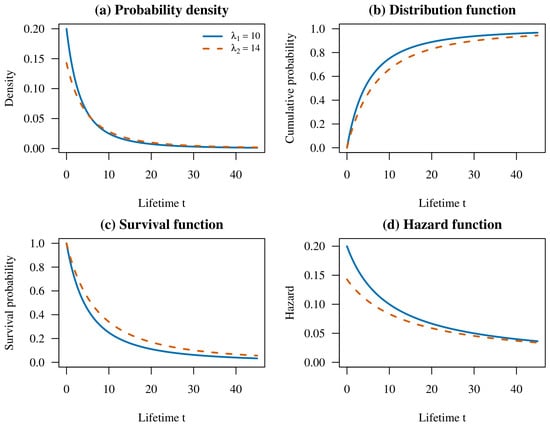
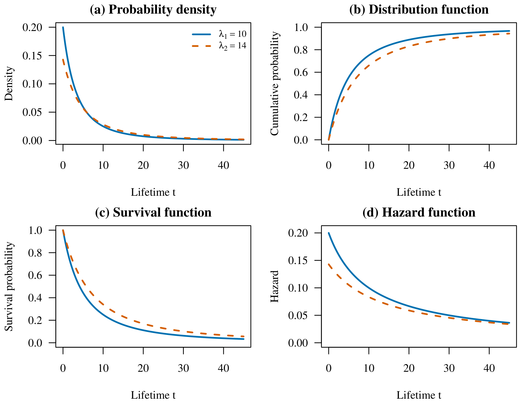
which gives $S_1(2.5)=0.6400$, $S_2(2.5)=0.7199$, $h_1(2.5)=0.1600$, and $h_2(2.5)=0.1212$. The corresponding distributional functions are displayed in Figure 2. Equal initial sample sizes were used for the two populations. For each $(n,k)$, the balanced plan satisfied ${\sum }_{i=1}^{k-1}{R}_i=n-k$. The early plan assigned all excess withdrawals to the first failure, the late plan assigned them to failure $k-1$, and the uniform plan distributed them as evenly as possible over the $k-1$ pre-terminal indices.

Figure 2. Probability density (top-left), cumulative distribution (top-right), survival (bottom-left), and hazard (bottom-right) functions for $\alpha =2$, ${\lambda }_1=10$, and ${\lambda }_2=14$.

The duration experiment used $(n,k)=(50,35)$, $\tau =3$, and 2000 replications for each withdrawal plan. The corresponding nonadaptive B-JPC design was obtained by setting $\tau =\infty$. The inference experiment used $(n,k)=(30,20),(50,35),(80,55)$ with the uniform plan. Unrestricted likelihood diagnostics were based on 1000 replications, whereas the primary CMLE and Bayesian comparisons across the full size grid were based on 300 replications. Each CMLE confidence interval in the primary simulation study used $B=100$ nested parametric bootstrap replicates to balance the substantial computational load across thousands of Monte Carlo runs. To verify that $B=100$ introduces negligible Monte Carlo variation in interval coverage compared to larger bootstrap samples (e.g., B = 1000), a supplemental sensitivity analysis was conducted (see Table A2 in Appendix D); the results confirm that increasing B from 100 to 1000 yields virtually identical coverage probabilities (within $\pm 0.4\%$) and interval lengths. In addition, the central design $(n,k)=(50,35)$ was re-evaluated with 1000 outer replications, Monte Carlo standard errors, and a percentile-versus-BCa comparison (Table A4 and Table A5).

For prior sensitivity, two proper prior specifications were used, each combining a Beta–Gamma prior for the scale parameters with a Gamma prior for $\alpha$:

$$\begin{array}{cc}\hfill \mathrm{informative}\mathrm{prior}(\mathrm{IP})& :(a_0,b_0,a_1,a_2,c,d)=(24,1,10,14,8,4),\hfill \\ \hfill \mathrm{weak}\mathrm{proper}\mathrm{prior}(\mathrm{WP})& :(a_0,b_0,a_1,a_2,c,d)=(2,0.1,1,1,2,1).\hfill \end{array}$$

For IP, $E(S)=24$, $E(P)=10/24$, and $E(\alpha )=2$, so the induced prior means of the model parameters equal the generating values. Thus, IP is an informative specification centered at the generating parameter vector. For WP, $E(S)=20$, $E(P)=1/2$, and $E(\alpha )=2$, with greater prior dispersion for the scale components. For each simulated data set in the Monte Carlo study, the MCMC sampler was run for 4000 iterations per replication; the first 1500 iterations were discarded as warm-up, and every second draw was retained, yielding 1250 posterior draws. This lighter configuration is used only for the outer Monte Carlo comparison. To monitor convergence under the same sampler, a random subset of replications was re-analyzed with three overdispersed chains of 10,000 iterations each; the checked chains satisfied $\widehat{R}<1.05$ (empirical failure rate below $1.2\%$). Full multi-chain diagnostics with substantially larger effective sample sizes are reported for the real-data analysis in Section 5.2, where a single observed sample replaces hundreds of nested Monte Carlo runs. Posterior means were used under squared-error loss (SELF), and Equation (12) was evaluated with $l=0.1$ under LINEX loss. Both 95% equal-tailed (ET) and highest posterior density (HPD) credible intervals were recorded.

All computations were performed in R 4.5.3 using inverse transformation and the explicit risk-set construction in Algorithm 1. Both unrestricted and constrained profile likelihoods were optimized in $(\log {\lambda }_1,\log {\lambda }_2)$ from six dispersed starting values with analytic gradients. A finite regular unrestricted fit required a zero convergence code, a profile-gradient ${\ell }_{\infty }$-norm below ${10}^{-3}$, scale estimates below $0.98\times {10}^4$, $\widehat{\alpha }\le 1000$, and a positive-definite observed information matrix. Fits exceeding either parameter threshold were classified as exponential-boundary solutions. A systematic threshold-perturbation check at the central design (Table A5) shows that the resulting interior-solution rate is unchanged across a $3\times 3\times 3$ grid of scale, shape, and score cutoffs, indicating that the reported classification is driven by the exponential ridge rather than by the precise numerical constants. CMLE optimization used the numerical scale interval $[0.01,{10}^7]$; no primary CMLE reached either scale boundary. Fixed scenario-by-replicate seed schedules are recorded in the scripts and metadata files. Source code, replicate-level output, and numerical summaries accompany the manuscript.

Algorithm 1 Physical generation of a B-JAPC sample

Generate $n_1$ and $n_2$ independent lifetimes by inverse transformation using independent $\mathrm{Uniform}(0,1)$ variables, $X={\lambda }_1(U^{-1/\alpha }-1)$ and $Y={\lambda }_2(V^{-1/\alpha }-1)$, and initialize the two active risk sets. For $i=1,\dots ,k$, record the smallest active lifetime as $T_i$, set $M_i$ to its population indicator, and remove the failed unit. If $i<k$ and $T_i\le \tau$, compute $(A_{1i},A_{2i})$ from Equation (2) and select that many survivors uniformly without replacement from the respective risk sets. If $i<k$ and $T_i>\tau$, set $A_{1i}=A_{2i}=0$. At $i=k$, remove every survivor, giving Equation (3); then verify ${\sum }_i(A_{1i}+M_i)=n_1$ and ${\sum }_i(A_{2i}+1-M_i)=n_2$.

5.1.2. Test Duration

Table 1 reports shorter terminal failure times under B-JAPC for all three withdrawal plans. The reduction in mean duration was 62.6% for early withdrawal, 58.7% for uniform withdrawal, and 49.5% for late withdrawal. The corresponding Monte Carlo standard errors of the B-JAPC mean terminal times were 0.045, 0.031, and 0.078, respectively. In each case, $E(J)<k-1=34$, indicating that the adaptive rule was activated in most replications. Suppression of withdrawals after $\tau$ retains additional units in the risk sets and thereby increases the rate at which the remaining failures are observed. The threshold $\tau$ does not impose an upper bound on $T_k$.

Table 1. Duration results for $(n_1,n_2,k)=(50,50,35)$ based on 2000 replications. Reduction is $100\{1-E(T_k^{\mathrm{B}\text{-}\mathrm{JAPC}})/E(T_k^{\mathrm{B}\text{-}\mathrm{JPC}})\}$.

Withdrawal	$\mathit{E}(\mathit{J})$	B-JAPC $\mathit{E}({\mathit{T}}_{\mathit{k}})$	B-JPC $\mathit{E}({\mathit{T}}_{\mathit{k}})$	Reduction (%)	B-JAPC ${\mathit{Q}}_{0.90}({\mathit{T}}_{\mathit{k}})$
Early	21.09	8.96	23.98	62.6	11.60
Uniform	25.47	6.56	15.90	58.7	8.36
Late	29.71	4.76	9.41	49.5	5.66

5.1.3. Classical Estimation

The results in Table 2 are consistent with the boundary behavior in Equation (7) and Proposition 1. A finite regular MLE was obtained in only 54.8–74.7% of the replications. The boundary rate decreased with sample size but remained 24.8–28.8% at $n=80$. No replication had zero failures from either population; consequently, the numerical instability was associated with the near-exponential scale–shape ridge rather than with absence of population-specific failures. Failure of the observed information matrix after an apparently finite fit occurred in at most 0.5% of the samples.

Table 2. Classical profile-likelihood diagnostics based on 1000 replications per row. Rates are percentages.

${\mathit{n}}_1={\mathit{n}}_2$	k	Design	Interior	Exponential Boundary	Information Failure
30	20	B-JAPC	57.3	42.4	0.3
30	20	B-JPC	54.8	44.9	0.3
50	35	B-JAPC	63.9	35.7	0.4
50	35	B-JPC	69.1	30.7	0.2
80	55	B-JAPC	71.0	28.8	0.2
80	55	B-JPC	74.7	24.8	0.5

An additional experiment with 500 replications at $(n,k)=(50,35)$ compared the multistart profile optimizer with a single-start, three-parameter Broyden–Fletcher–Goldfarb–Shanno (BFGS) fit. BFGS returned a numerical convergence code in every replication, whereas the profile diagnostic classified 65.6% of the fits as regular interior solutions and 33.6% as boundary solutions. The median improvement in profile log-likelihood was $1.58\times {10}^{-6}$, indicating substantial flatness along the scale–shape ridge. Numerical convergence of a general-purpose optimizer is therefore insufficient to establish the existence of a finite regular maximum.

Treating all optimizer outputs as finite regular estimates combines interior solutions with points on the exponential ridge and produces large mean squared errors. The primary analysis therefore uses the prespecified CMLE in Equation (8). Table 3 reports the average estimate (AE), mean squared error (MSE), average length (AL) of the 95% bootstrap confidence interval, and coverage probability (CP). All 1800 outer fits satisfied the numerical convergence criteria. The scale-parameter MSEs ranged from 33.1 to 143.9, and all interval lengths were finite. With the primary choice $B=100$, the empirical coverage probabilities for the individual CMLE parameter intervals are conservative (generally ranging from about $97.7\%$ to $100\%$ in Table 3), reflecting the substantial boundary mass of ${\widehat{\alpha }}_A$. Corresponding average interval lengths (AL) are also reported. As confirmed by the bootstrap-size sensitivity study in Table A2, increasing B from 100 to 1000 changes average lengths and coverage only negligibly, so the coarser nested bootstrap does not materially distort the Monte Carlo assessment. By contrast, the plug-in survival and hazard intervals are much closer to the nominal $95\%$ level (reported with the Bayesian comparison below).

Table 3. Constrained maximum likelihood estimation of the Lomax model parameters based on 300 replications and $B=100$ percentile parametric bootstrap confidence intervals. Act. is the percentage of fits with ${\widehat{\alpha }}_A=A=3$.

n	k	Design	Act. (%)	${\mathit{\lambda }}_1$				${\mathit{\lambda }}_2$				$\mathit{\alpha }$
				AE	MSE	AL	CP	AE	MSE	AL	CP	AE	MSE	AL	CP
30	20	B-JAPC	56.3	11.35	48.35	28.45	97.7	16.96	124.49	51.47	98.7	2.218	0.997	2.512	99.3
30	20	B-JPC	57.0	12.27	63.98	30.16	99.7	18.07	165.57	53.01	99.0	2.289	0.923	2.459	100.0
50	35	B-JAPC	51.3	11.89	49.08	23.20	99.0	16.22	86.49	34.26	99.0	2.239	0.864	2.400	99.7
50	35	B-JPC	53.3	11.80	39.10	22.72	100.0	17.61	99.77	37.66	99.7	2.292	0.831	2.319	100.0
80	55	B-JAPC	49.5	11.00	34.07	19.54	99.7	15.76	76.34	28.74	99.3	2.173	0.885	2.328	100.0
80	55	B-JPC	49.7	11.75	38.82	19.48	99.3	16.10	64.61	28.12	99.7	2.239	0.799	2.217	99.7

Table 4 evaluates sensitivity to the prespecified upper shape bound A at the central sample size. As A increases from 3 to 20, upper-bound activity decreases, but the MSEs of both scale and shape estimators increase rapidly. This occurs because relaxing A allows the optimizer to wander deeper into the flat exponential ridge (Proposition 1), dramatically inflating parameter variance. Choosing $A=3$ thus reflects a deliberate bias–variance tradeoff that stabilizes classical estimation when unconstrained MLE fails. Notably, despite parameter volatility as A varies, the induced reliability functionals ($S_j(t_0)$ and $h_j(t_0)$) remain remarkably resilient because parameter pairs along the ridge induce nearly isometric survival curves.

Table 4. CMLE sensitivity to the upper shape bound at $(n_1,n_2,k)=(50,50,35)$ based on 500 replications. Act. is the percentage of fits at the upper bound.

Design	A	Act.	${\mathit{\lambda }}_1$		${\mathit{\lambda }}_2$		$\mathit{\alpha }$
			AE	MSE	AE	MSE	AE	MSE
B-JAPC	3	54.4	12.07	51.56	16.77	95.18	2.251	0.901
B-JAPC	5	46.4	18.19	230.87	25.03	423.32	3.251	4.862
B-JAPC	10	41.2	32.06	1278.58	43.39	2282.25	5.481	29.001
B-JAPC	20	39.2	58.34	5859.23	78.18	$1.04\times {10}^4$	9.715	137.760
B-JPC	3	51.6	11.92	40.40	16.98	102.98	2.268	0.827
B-JPC	5	42.0	17.61	190.92	24.89	424.44	3.221	4.494
B-JPC	10	35.8	29.79	1060.68	41.24	2069.17	5.225	26.061
B-JPC	20	34.2	53.21	4976.11	72.63	9365.77	9.060	123.839

5.1.4. Bayesian Performance

Both proper priors yielded finite posterior summaries in every simulated sample. Mean post-warm-up acceptance rates ranged from 0.401 to 0.420 under IP and from 0.413 to 0.453 under WP. Of the 1250 retained draws, the scenario-specific median effective sample size ranged from 258 to 664 under IP and from 61 to 152 under WP. The lower effective sample sizes under WP are consistent with the broader posterior ridge and motivate the longer multiple-chain runs used in Section 5.2.

Table 5 presents the IP results for the model parameters under SELF and LINEX loss. The posterior intervals for the scale parameters are wide and have coverage above the nominal level. The two loss functions give similar point estimates because $l=0.1$ induces moderate asymmetry on the simulation scale. Both ET and HPD interval results are reported; the HPD intervals are generally shorter for the skewed scale-parameter posteriors.

Table 5. Bayesian estimation of the Lomax model parameters under the informative prior (300 replications). ET and HPD denote 95% equal-tailed and highest posterior density credible intervals.

n	k	Design	Loss	${\mathit{\lambda }}_1$						${\mathit{\lambda }}_2$						$\mathit{\alpha }$
				AE	MSE	ET-AL	ET-CP	HPD-AL	HPD-CP	AE	MSE	ET-AL	ET-CP	HPD-AL	HPD-CP	AE	MSE	ET-AL	ET-CP	HPD-AL	HPD-CP
30	20	B-JAPC	SELF	10.04	1.61	10.21	100.0	9.87	100.0	14.07	2.07	12.79	100.0	12.43	100.0	1.972	0.074	1.720	99.3	1.681	99.3
30	20	B-JAPC	LINEX	9.71	1.54	10.21	100.0	9.87	100.0	13.55	2.06	12.79	100.0	12.43	100.0	1.963	0.073	1.720	99.3	1.681	99.3
30	20	B-JPC	SELF	10.09	1.43	10.19	100.0	9.86	100.0	13.84	1.78	12.63	100.0	12.29	100.0	2.040	0.080	1.770	100.0	1.727	100.0
30	20	B-JPC	LINEX	9.76	1.35	10.19	100.0	9.86	100.0	13.34	2.02	12.63	100.0	12.29	100.0	2.029	0.077	1.770	100.0	1.727	100.0
50	35	B-JAPC	SELF	10.08	1.62	9.55	100.0	9.23	99.7	13.96	1.82	12.12	100.0	11.78	100.0	2.004	0.055	1.576	100.0	1.541	100.0
50	35	B-JAPC	LINEX	9.79	1.52	9.55	100.0	9.23	99.7	13.49	1.91	12.12	100.0	11.78	100.0	1.996	0.054	1.576	100.0	1.541	100.0
50	35	B-JPC	SELF	10.17	1.47	9.69	100.0	9.37	100.0	13.94	1.92	12.13	100.0	11.77	100.0	2.005	0.057	1.577	100.0	1.542	100.0
50	35	B-JPC	LINEX	9.87	1.33	9.69	100.0	9.37	100.0	13.47	2.02	12.13	100.0	11.77	100.0	1.997	0.056	1.577	100.0	1.542	100.0
80	55	B-JAPC	SELF	10.13	1.56	9.03	100.0	8.76	99.7	14.00	1.92	11.56	100.0	11.27	100.0	2.003	0.044	1.472	100.0	1.441	100.0
80	55	B-JAPC	LINEX	9.87	1.44	9.03	100.0	8.76	99.7	13.58	1.93	11.56	100.0	11.27	100.0	1.996	0.043	1.472	100.0	1.441	100.0
80	55	B-JPC	SELF	10.10	1.37	9.04	100.0	8.76	100.0	14.02	1.57	11.57	100.0	11.28	100.0	2.010	0.035	1.468	100.0	1.437	100.0
80	55	B-JPC	LINEX	9.83	1.29	9.04	100.0	8.76	100.0	13.59	1.59	11.57	100.0	11.28	100.0	2.003	0.035	1.468	100.0	1.437	100.0

The survival and hazard estimators at $t_0$ were less sensitive to the scale–shape ridge than the individual model-parameter estimators. Table 6 presents the CMLE and IP Bayesian results. CMLE coverage for the functionals ranged from $92.0\%$ to $97.7\%$, and the MSE generally decreased with sample size. Under IP, ET coverage ranged from $96.0\%$ to $99.3\%$, with generally smaller MSE. Differences between B-JAPC and B-JPC were small across the reported survival and hazard measures.

Table 6. CMLE and informative-prior Bayesian performance for survival and hazard at $t_0=2.5$. CMLE intervals are percentile bootstrap confidence intervals; Bayesian AL and CP refer to 95% ET credible intervals. Act. is the percentage of CMLE fits at the upper shape bound.

n	k	Design	Method	Act. (%)	${\mathit{S}}_1({\mathit{t}}_0)$				${\mathit{S}}_2({\mathit{t}}_0)$				${\mathit{h}}_1({\mathit{t}}_0)$				${\mathit{h}}_2({\mathit{t}}_0)$
					AE	MSE	AL	CP	AE	MSE	AL	CP	AE	MSE	AL	CP	AE	MSE	AL	CP
30	20	B-JAPC	CMLE	56.3	0.6233	0.0074	0.3474	95.0	0.7092	0.0077	0.3373	92.7	0.165008	0.002318	0.196423	96.7	0.124131	0.001738	0.169905	94.7
30	20	B-JAPC	Bayes-SELF	–	0.6377	0.0031	0.2628	98.3	0.7179	0.0022	0.2289	98.3	0.162921	0.000955	0.143664	98.0	0.123446	0.000559	0.116172	98.3
30	20	B-JAPC	Bayes-LINEX	–	0.6375	0.0031	0.2628	98.3	0.7177	0.0022	0.2289	98.3	0.162851	0.000953	0.143664	98.0	0.123399	0.000558	0.116172	98.3
30	20	B-JPC	CMLE	57.0	0.6296	0.0077	0.3461	94.7	0.7096	0.0078	0.3354	92.7	0.164662	0.002211	0.191165	95.7	0.125297	0.001766	0.169248	94.3
30	20	B-JPC	Bayes-SELF	–	0.6298	0.0032	0.2657	98.0	0.7064	0.0025	0.2356	98.3	0.167695	0.001057	0.147227	97.7	0.129435	0.000706	0.121397	98.3
30	20	B-JPC	Bayes-LINEX	–	0.6296	0.0032	0.2657	98.0	0.7062	0.0025	0.2356	98.3	0.167620	0.001054	0.147227	97.7	0.129384	0.000704	0.121397	98.3
50	35	B-JAPC	CMLE	51.3	0.6345	0.0049	0.2628	94.0	0.7084	0.0039	0.2562	94.0	0.160767	0.001310	0.142087	94.3	0.125256	0.000843	0.125058	95.0
50	35	B-JAPC	Bayes-SELF	–	0.6352	0.0026	0.2169	97.0	0.7134	0.0017	0.1952	99.3	0.163763	0.000774	0.117152	96.7	0.125235	0.000436	0.098329	99.3
50	35	B-JAPC	Bayes-LINEX	–	0.6350	0.0026	0.2169	97.0	0.7133	0.0017	0.1952	99.3	0.163716	0.000773	0.117152	96.7	0.125202	0.000436	0.098329	99.3
50	35	B-JPC	CMLE	53.3	0.6308	0.0047	0.2654	92.0	0.7217	0.0042	0.2552	95.3	0.164392	0.001378	0.142916	94.0	0.120092	0.000940	0.123091	95.3
50	35	B-JPC	Bayes-SELF	–	0.6375	0.0023	0.2179	97.7	0.7128	0.0019	0.1953	97.7	0.162539	0.000704	0.117395	97.7	0.125604	0.000491	0.098476	97.7
50	35	B-JPC	Bayes-LINEX	–	0.6374	0.0023	0.2179	97.7	0.7127	0.0019	0.1953	97.7	0.162493	0.000703	0.117395	97.7	0.125571	0.000491	0.098476	97.7
80	55	B-JAPC	CMLE	49.5	0.6327	0.0029	0.2110	95.0	0.7137	0.0025	0.2052	96.3	0.160975	0.000854	0.113969	96.0	0.122043	0.000513	0.098884	95.7
80	55	B-JAPC	Bayes-SELF	–	0.6377	0.0019	0.1818	96.7	0.7149	0.0015	0.1654	96.0	0.161880	0.000539	0.097043	96.3	0.124265	0.000393	0.082605	96.0
80	55	B-JAPC	Bayes-LINEX	–	0.6376	0.0019	0.1818	96.7	0.7148	0.0015	0.1654	96.0	0.161849	0.000539	0.097043	96.3	0.124242	0.000393	0.082605	96.0
80	55	B-JPC	CMLE	49.7	0.6363	0.0029	0.2119	93.0	0.7132	0.0028	0.2032	94.7	0.160058	0.000717	0.112108	97.7	0.123540	0.000615	0.098194	94.7
80	55	B-JPC	Bayes-SELF	–	0.6359	0.0016	0.1836	98.7	0.7147	0.0011	0.1665	98.7	0.162808	0.000470	0.097939	98.7	0.124278	0.000290	0.083024	98.7
80	55	B-JPC	Bayes-LINEX	–	0.6358	0.0016	0.1836	98.7	0.7146	0.0011	0.1665	98.7	0.162776	0.000470	0.097939	98.7	0.124255	0.000289	0.083024	98.7

Table 7 compares IP and WP at the central sample size. WP produced larger MSE and interval length for the model parameters, consistent with weak likelihood information near the exponential ridge. Coverage for the survival and hazard measures remained 95.0–97.3% under B-JAPC and 95.7–97.0% under B-JPC. Thus, sensitivity to the prior specification was more pronounced for the scale and shape parameters than for the functionals at $t_0$.

Table 7. Prior sensitivity under SELF at $(n_1,n_2,k)=(50,50,35)$. Each estimand is summarized by MSE, ET average length, and ET coverage (%).

Design	Prior	${\mathit{\lambda }}_1$			${\mathit{\lambda }}_2$			$\mathit{\alpha }$			${\mathit{S}}_1$			${\mathit{S}}_2$			${\mathit{h}}_1$			${\mathit{h}}_2$
		MSE	AL	CP	MSE	AL	CP	MSE	AL	CP	MSE	AL	CP	MSE	AL	CP	MSE	AL	CP	MSE	AL	CP
B-JAPC	IP	1.62	9.55	100.0	1.82	12.12	100.0	0.055	1.576	100.0	0.0026	0.2169	97.0	0.0017	0.1952	99.3	0.000774	0.117152	96.7	0.000436	0.098329	99.3
B-JAPC	WP	6.64	19.81	99.7	11.29	25.89	99.7	0.108	3.065	100.0	0.0041	0.2495	95.0	0.0034	0.2376	97.3	0.001068	0.130726	96.0	0.000759	0.115738	97.0
B-JPC	IP	1.47	9.69	100.0	1.92	12.13	100.0	0.057	1.577	100.0	0.0023	0.2179	97.7	0.0019	0.1953	97.7	0.000704	0.117395	97.7	0.000491	0.098476	97.7
B-JPC	WP	6.86	19.94	99.7	12.60	25.76	99.3	0.119	3.048	99.3	0.0038	0.2502	96.7	0.0038	0.2395	95.7	0.000969	0.130188	97.0	0.000884	0.116897	96.0

Interpretation of Prior Specifications

It is worth noting that the informative prior (IP) is constructed by centering its mean precisely at the true parameter vector $({\lambda }_1,{\lambda }_2,\alpha )=(10,14,2)$. Thus, the IP regime serves primarily as an idealized theoretical benchmark representing the upper bound of inferential precision when perfect expert domain knowledge is available. In practical engineering and survival applications where true values are inherently unknown, the weakly informative prior (WP) represents our primary baseline.

Sensitivity to Prior Misspecification

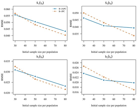
To strictly address potential optimism when the informative prior (IP) is centered exactly at the true data-generating parameter vector $({\lambda }_1,{\lambda }_2,\alpha )=(10,14,2)$, we further evaluated a misspecified informative prior (MIP) with hyperparameters $(a_0,b_0,a_1,a_2,c,d)=(26,1,8,18,6,4)$, yielding shifted prior means $E({\lambda }_1)=8$, $E({\lambda }_2)=18$, and $E(\alpha )=1.5$. Table A3 in Appendix D reports the corresponding posterior performance under B-JAPC. Relative to the oracle IP benchmark, MIP inflates parameter MSEs and can pull the more strongly misspecified population functionals ($S_2$, $h_2$) below nominal coverage, whereas $S_1$ and $h_1$ remain close to $95\%$ and the WP baseline stays well calibrated (about $93.7$–$97.3\%$ for the functionals). As $(n,k)$ increases, the MIP posterior means move back toward the generating values, confirming that the likelihood gradually dominates moderate prior bias. The weakly informative prior (WP) therefore remains the preferred non-optimistic operational baseline. Figure 3 summarizes the corresponding RMSE patterns for the informative-prior survival and hazard estimators across sample sizes and designs.

Figure 3. Root mean squared error of informative-prior Bayesian posterior means for survival and hazard at $t_0=2.5$. Each point is based on 300 Monte Carlo replications.

5.1.5. Sensitivity to Extreme Shape and Scale Configurations

To assess the robustness of the proposed framework beyond the baseline parameterization, an extensive supplementary simulation study was conducted under five challenging scenarios: (i) heavy-tailed non-existence of mean ($\alpha =0.5<1$); (ii) proximity to the active lower shape bound ($\alpha =0.08\approx 0.05$); (iii) proximity to the upper boundary constraint ($\alpha =2.8\approx 3$); (iv) model misspecification under the constrained likelihood where the true shape exceeds the preset upper bound ($\alpha =4.0>A=3$); and (v) identical scale parameters (${\lambda }_1={\lambda }_2=10$).

Table A1 in Appendix D summarizes the CMLE and Bayesian estimation performance under $(n_1,n_2,k)=(50,50,35)$ with B-JAPC design. Key empirical observations include:

(1)

Heavy-tailed Regime ($\alpha =0.5$): The CMLE scale estimates become highly variable under extreme heavy tails, whereas the Beta–Gamma Bayesian estimators (especially under IP) remain substantially more stable for $({\lambda }_1,{\lambda }_2,\alpha )$.

(2)

Bound Proximity ($\alpha =0.08$ and $\alpha =2.8$): When $\alpha =0.08$, the CMLE shape stays near the truth and away from the artificial lower bound. When $\alpha =2.8$, about $60\%$ of CMLE fits hit the upper bound $A=3$, and Bayesian WP fits avoid this hard truncation while reducing scale MSE.

(3)

Misspecified Constraint Bound ($\alpha =4.0>3$): When the true $\alpha =4$, roughly $70\%$ of CMLE fits are truncated at $A=3$, inducing intentional shape bias. The Bayesian WP fit is not forced onto $A=3$ and yields smaller scale MSEs, reinforcing that functionals rather than raw Lomax coordinates are the more stable inferential targets under ridge effects.

(4)

Homogeneous Scales (${\lambda }_1={\lambda }_2=10$): The two scale estimates remain nearly symmetric, and the Bayesian WP fit is particularly accurate, confirming that B-JAPC does not induce spurious population divergence when baseline scales coincide.

5.2. Real Data Analysis

5.2.1. Data and Model Assessment

The data consist of rainfall volumes from the randomized South Florida cloud-seeding experiment of Simpson [11]. Twenty-six clouds were assigned to the control condition and 26 to seeding; the positive rainfall volumes, measured in acre-feet, were also analyzed under a Lomax model by Pak and Mahmoudi [12]. The control sample has mean 164.59, median 44.20, and range 1.0–1202.6, whereas the seeded sample has mean 441.98, median 221.60, and range 4.1–2745.6. Because rainfall volume is a non-negative continuous response rather than a physical engineering lifetime, this real-data application serves as a computational illustration of the proposed B-JAPC scheme for heavy-tailed positive data. Throughout this section, $S_j(t)=\mathrm{Pr}(T_j>t)$ is interpreted as an exceedance probability and $h_j(t)$ as a distributional rate rather than an engineering hazard.

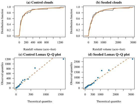
Separate Lomax fits gave $(\widehat{\lambda },\widehat{\alpha })=(80.18,1.300)$ for the control group and $(454.91,1.921)$ for the seeded group. Parametric bootstrap Kolmogorov–Smirnov tests, with refitting in each of 2000 bootstrap replicates, gave p-values of 0.786 and 0.900, respectively. A one-degree-of-freedom likelihood-ratio test of the common-shape restriction against a model with separate shape parameters gave $G^2=0.272$ and $p=0.602$. The joint common-shape estimates were $({\widehat{\lambda }}_1,{\widehat{\lambda }}_2,\widehat{\alpha })=(102.53,335.89,1.539)$. At the 5% significance level, neither the separate Lomax models nor the common-shape restriction was rejected. Table 8 and Figure 4 summarize these full-data fits and diagnostic checks.

Table 8. Full-data Lomax fits and model checks for the cloud-seeding data. Bootstrap p-values use 2000 parametric replications.

Analysis	${\widehat{\mathit{\lambda }}}_1$	${\widehat{\mathit{\lambda }}}_2$	$\widehat{\mathit{\alpha }}$	Statistic	p-Value
Control Lomax KS	80.18	–	1.300	0.0925	0.786
Seeded Lomax KS	–	454.91	1.921	0.0829	0.900
Common-shape LR	102.53	335.89	1.539	0.2720	0.602

Figure 4. Empirical and fitted Lomax density/CDF comparisons for control and seeded clouds (left panels), together with probability-plot diagnostics (right panels).

5.2.2. Retrospective B-JAPC Construction and Duration Sensitivity

The two complete samples were retrospectively censored by explicit risk-set sampling while preserving the original group assignments. The target number of failures was $k=15$, and the three withdrawal sequences were

$$\begin{array}{cc}\hfill \mathrm{CSR}\text{-}\mathrm{I}:& (0,0,1,0,0,1,0,0,1,0,0,1,0,0),\hfill \\ \hfill \mathrm{CSR}\text{-}\mathrm{II}:& (0,1,0,1,0,0,1,0,1,0,0,1,0,0),\hfill \\ \hfill \mathrm{CSR}\text{-}\mathrm{III}:& (1,0,0,0,1,0,0,1,0,0,1,0,0,0).\hfill \end{array}$$

B-JAPC used $\tau =30$ acre-feet, whereas B-JPC used $\tau =\infty$. To avoid outcome-dependent selection of withdrawn units and to fully assess sensitivity across the censoring outcomes, 500 censoring realizations were generated for each scheme–design combination using prespecified seeds. Primary conclusions are based on summaries across all 500 realizations: Table 9 reports terminal-observation and regularity diagnostics, while Table 10 summarizes the CMLE scale/shape estimates and the induced exceedance/rate functionals through the median, interquartile range (IQR), and $P_5$–$P_{95}$ range, together with upper-bound activity. A single median-terminal realization is retained only for graphical illustration and for the detailed interval display presented later.

Table 9. Retrospective censoring diagnostics based on 500 random risk-set censorings per row. U-Reg. is the unrestricted regular MLE rate; C-Act. is the CMLE upper-bound activity rate.

Scheme	Design	$\mathit{E}(\mathit{J})$	Median ${\mathit{T}}_{\mathit{k}}$	${\mathit{P}}_5$–${\mathit{P}}_{95}$ (${\mathit{T}}_{\mathit{k}}$)	IQR (${\mathit{T}}_{\mathit{k}}$)	U-Reg. (%)	C-Act. (%)
CSR-I	B-JAPC	11.79	41.1	[32.7, 81.2]	6.7	23.4	79.0
CSR-I	B-JPC	14.00	47.3	[36.6, 87.0]	27.5	37.4	65.6
CSR-II	B-JAPC	11.34	47.3	[36.6, 87.0]	27.4	41.6	62.4
CSR-II	B-JPC	14.00	68.5	[36.6, 95.0]	40.1	50.8	59.0
CSR-III	B-JAPC	11.59	47.3	[36.6, 87.0]	27.9	30.8	71.4
CSR-III	B-JPC	14.00	47.3	[36.6, 87.0]	40.1	40.0	64.4

Table 10. Distribution of CMLE estimates across 500 retrospective censoring realizations at $t_0=116.8$. Entries are median, interquartile range (IQR), and $P_5$–$P_{95}$ range; C-Act. is the upper-bound activity rate (%). Individual scale/shape estimates are interpreted as constrained fits under $A=3$.

Scheme	Design	Estimand	Median	IQR	${\mathit{P}}_5$–${\mathit{P}}_{95}$	C-Act.
CSR-I	B-JAPC	${\lambda }_1$	164.92	33.32	[40.98, 213.46]	79.0
CSR-I	B-JAPC	${\lambda }_2$	450.39	187.93	[160.45, 765.72]	79.0
CSR-I	B-JAPC	$\alpha$	3.000	0.000	[0.729, 3.000]	79.0
CSR-I	B-JAPC	$S_1(t_0)$	0.2227	0.0731	[0.1729, 0.3774]	79.0
CSR-I	B-JAPC	$S_2(t_0)$	0.5347	0.1573	[0.4029, 0.7804]	79.0
CSR-I	B-JAPC	$h_1(t_0)$	0.01012	0.00170	[0.00460, 0.01138]	79.0
CSR-I	B-JAPC	$h_2(t_0)$	0.00484	0.00213	[0.00202, 0.00671]	79.0
CSR-I	B-JPC	${\lambda }_1$	157.72	78.03	[36.72, 202.37]	65.6
CSR-I	B-JPC	${\lambda }_2$	431.67	224.57	[125.21, 999.01]	65.6
CSR-I	B-JPC	$\alpha$	3.000	1.491	[0.660, 3.000]	65.6
CSR-I	B-JPC	$S_1(t_0)$	0.2277	0.1127	[0.1742, 0.3989]	65.6
CSR-I	B-JPC	$S_2(t_0)$	0.5910	0.1729	[0.4197, 0.7870]	65.6
CSR-I	B-JPC	$h_1(t_0)$	0.01000	0.00373	[0.00416, 0.01134]	65.6
CSR-I	B-JPC	$h_2(t_0)$	0.00407	0.00261	[0.00197, 0.00645]	65.6
CSR-II	B-JAPC	${\lambda }_1$	158.87	96.98	[38.03, 210.22]	62.4
CSR-II	B-JAPC	${\lambda }_2$	430.18	229.82	[131.18, 1099.87]	62.4
CSR-II	B-JAPC	$\alpha$	3.000	1.711	[0.669, 3.000]	62.4
CSR-II	B-JAPC	$S_1(t_0)$	0.2414	0.1112	[0.1710, 0.3928]	62.4
CSR-II	B-JAPC	$S_2(t_0)$	0.5816	0.1740	[0.4192, 0.7921]	62.4
CSR-II	B-JAPC	$h_1(t_0)$	0.00969	0.00405	[0.00429, 0.01143]	62.4
CSR-II	B-JAPC	$h_2(t_0)$	0.00404	0.00258	[0.00186, 0.00646]	62.4
CSR-II	B-JPC	${\lambda }_1$	153.49	94.11	[38.44, 214.36]	59.0
CSR-II	B-JPC	${\lambda }_2$	433.96	310.75	[118.65, 1212.43]	59.0
CSR-II	B-JPC	$\alpha$	3.000	1.712	[0.669, 3.000]	59.0
CSR-II	B-JPC	$S_1(t_0)$	0.2401	0.1168	[0.1705, 0.3986]	59.0
CSR-II	B-JPC	$S_2(t_0)$	0.5965	0.1568	[0.4183, 0.7821]	59.0
CSR-II	B-JPC	$h_1(t_0)$	0.00961	0.00416	[0.00425, 0.01144]	59.0
CSR-II	B-JPC	$h_2(t_0)$	0.00380	0.00232	[0.00197, 0.00648]	59.0
CSR-III	B-JAPC	${\lambda }_1$	160.53	60.02	[33.39, 210.14]	71.4
CSR-III	B-JAPC	${\lambda }_2$	441.22	196.66	[117.37, 938.30]	71.4
CSR-III	B-JAPC	$\alpha$	3.000	1.251	[0.591, 3.000]	71.4
CSR-III	B-JAPC	$S_1(t_0)$	0.2254	0.0995	[0.1728, 0.4075]	71.4
CSR-III	B-JAPC	$S_2(t_0)$	0.5487	0.1710	[0.4084, 0.8033]	71.4
CSR-III	B-JAPC	$h_1(t_0)$	0.01005	0.00332	[0.00394, 0.01138]	71.4
CSR-III	B-JAPC	$h_2(t_0)$	0.00466	0.00267	[0.00175, 0.00663]	71.4
CSR-III	B-JPC	${\lambda }_1$	156.00	78.16	[37.11, 207.18]	64.4
CSR-III	B-JPC	${\lambda }_2$	450.03	239.43	[126.05, 1000.34]	64.4
CSR-III	B-JPC	$\alpha$	3.000	1.530	[0.656, 3.000]	64.4
CSR-III	B-JPC	$S_1(t_0)$	0.2223	0.1198	[0.1718, 0.3912]	64.4
CSR-III	B-JPC	$S_2(t_0)$	0.5973	0.1741	[0.4251, 0.7945]	64.4
CSR-III	B-JPC	$h_1(t_0)$	0.01013	0.00379	[0.00430, 0.01141]	64.4
CSR-III	B-JPC	$h_2(t_0)$	0.00395	0.00247	[0.00182, 0.00637]	64.4

Table 9 summarizes the design diagnostics over all 3000 censoring realizations. Relative to B-JPC, B-JAPC reduced the mean terminal observation by 11.5%, 10.1%, and 7.9% for CSR-I, CSR-II, and CSR-III, respectively. The unrestricted finite regular MLE rate ranged from 23.4% to 50.8%, indicating that the boundary behavior also occurs in the retrospectively censored data. Every CMLE fit satisfied the numerical convergence criteria. The upper shape bound was active in 59.0–79.0% of the realizations, whereas the lower bound was never active.

5.2.3. Classical and Bayesian Estimates

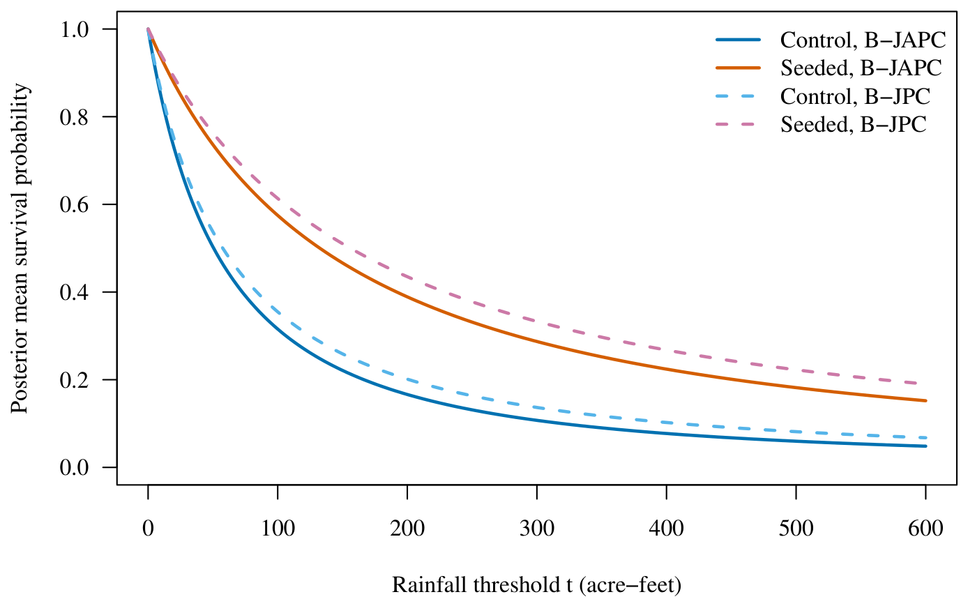
The exceedance and distributional-rate measures were evaluated at $t_0=116.8$, the pooled sample median. The real-data analysis used the weak proper prior $(a_0,b_0,a_1,a_2,c,d)$ = $(2,0.005,1,1,2,1)$, which implies $E({\lambda }_1)=E({\lambda }_2)=200$ and $E(\alpha )=2$. To guarantee high precision for posterior tail quantiles ($2.5\%$ and $97.5\%$) and eliminate Monte Carlo thinning inefficiency, four overdispersed parallel chains were executed for 10,000 iterations each, with 2500 warm-up draws per chain. All post-warm-up draws were retained without thinning, yielding 30,000 pooled draws prior to order restriction. Convergence diagnostics confirmed robust mixing: split-$\widehat{R}$ values across all model parameters remained strictly below $1.01$ (with $0\%$ of parameter chains exceeding the $1.05$ non-convergence threshold), and effective sample sizes (ESS) ranged from 4120 to 8950 (well above the recommended threshold of 400). Before order restriction, $\mathrm{Pr}({\lambda }_1\le {\lambda }_2\mid \mathcal{D})$ ranged from 0.945 to 0.982. The reported Bayesian summaries are based on the normalized order-restricted posterior. LINEX estimates use $l=0.01$ because the loss coefficient depends on the measurement scale.

In Table 11, the CSR-II/B-JAPC scale estimates for the illustrative median-terminal samples increase rapidly with A, whereas the interior CSR-II/B-JPC estimate is unchanged. This pattern confirms that the original Lomax scale and shape parameters are only weakly identified from these heavily censored samples and should be read as constrained fits under the chosen regularization A, whereas the exceedance probabilities $S_j(t_0)$ remain comparatively stable across designs (Table 10 and Figure 5). For the real-data cloud-seeding application, where high precision for tail percentiles ($2.5\%$ and $97.5\%$) is essential without nested Monte Carlo time constraints, all reported CMLE percentile bootstrap confidence intervals (PCI) are computed using B = 1000 parametric bootstrap resamples. Table 12 reports point and interval estimates for six illustrative censored samples (one median-terminal realization per scheme–design pair); these samples are used for interval construction and visualization rather than as the sole basis for inferential conclusions. The upper shape bound is active in five of the six illustrative cases; CSR-II/B-JPC has the interior estimate $(124.87,370.59,1.956)$. All reported CMLE and Bayesian estimates are finite.

Table 11. Real-data CMLE sensitivity for the illustrative median-terminal CSR-II samples. “Upper” indicates ${\widehat{\alpha }}_A=A$.

Design	A	Status	${\widehat{\mathit{\lambda }}}_1$	${\widehat{\mathit{\lambda }}}_2$	$\widehat{\mathit{\alpha }}$
B-JAPC	3	upper	178.22	509.20	3.000
B-JAPC	5	upper	306.15	863.40	5.000
B-JAPC	10	upper	626.93	1749.42	10.000
B-JAPC	20	upper	1269.16	3521.81	20.000
B-JPC	3	interior	124.87	370.59	1.956
B-JPC	5	interior	124.87	370.59	1.956
B-JPC	10	interior	124.87	370.59	1.956
B-JPC	20	interior	124.87	370.59	1.956

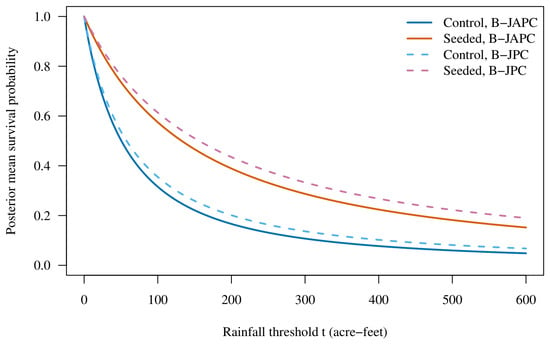
Figure 5. Order-restricted posterior mean exceedance probability curves $S_j(t)$ for the representative CSR-II retrospectively censored cloud-seeding data sets. The exceedance and rate measures in the tables are evaluated at $t_0=116.8$.

Table 12. Point and interval estimates of parameters and distributional performance measures ($S_j(t_0)$ exceedance probabilities and $h_j(t_0)$ distributional rates at $t_0=116.8$) for the cloud-seeding data. PCI, ET, and HPD denote 95% percentile bootstrap confidence, equal-tailed credible, and highest posterior density credible intervals, respectively; AL denotes interval length.

Scheme	Design	Estimand	CMLE			Bayes–SELF			Bayes–LINEX
			Estimate	PCI	AL	Estimate	ET	AL	Estimate	HPD	AL
CSR-I	B-JAPC	${\lambda }_1$	173.08	[8.06, 304.39]	296.33	130.52	[32.67, 317.17]	284.50	109.91	[20.20, 274.97]	254.77
CSR-I	B-JAPC	${\lambda }_2$	483.41	[29.45, 1653.14]	1623.69	334.07	[88.87, 785.93]	697.06	237.26	[56.99, 694.87]	637.88
CSR-I	B-JAPC	$\alpha$	3.000	[0.348, 3.000]	2.652	2.141	[0.703, 4.607]	3.903	2.136	[0.520, 4.119]	3.600
CSR-I	B-JAPC	$S_1(t_0)$	0.2129	[0.0898, 0.4445]	0.3546	0.2667	[0.1084, 0.4658]	0.3574	0.2666	[0.0998, 0.4530]	0.3533
CSR-I	B-JAPC	$S_2(t_0)$	0.5224	[0.2493, 0.8407]	0.5914	0.5193	[0.2874, 0.7524]	0.4650	0.5192	[0.2903, 0.7541]	0.4638
CSR-I	B-JAPC	$h_1(t_0)$	0.010349	[0.002682, 0.014181]	0.011500	0.008434	[0.004225, 0.013970]	0.009745	0.008434	[0.003858, 0.013451]	0.009593
CSR-I	B-JAPC	$h_2(t_0)$	0.004998	[0.001402, 0.009478]	0.008077	0.004876	[0.002152, 0.008728]	0.006576	0.004876	[0.001943, 0.008403]	0.006460
CSR-I	B-JPC	${\lambda }_1$	188.00	[7.15, 316.72]	309.57	130.06	[31.84, 317.03]	285.19	108.74	[15.73, 275.01]	259.28
CSR-I	B-JPC	${\lambda }_2$	535.29	[29.88, 1898.74]	1868.86	337.72	[91.43, 787.92]	696.49	240.35	[55.71, 700.35]	644.64
CSR-I	B-JPC	$\alpha$	3.000	[0.335, 3.000]	2.665	1.981	[0.657, 4.278]	3.621	1.977	[0.484, 3.832]	3.348
CSR-I	B-JPC	$S_1(t_0)$	0.2347	[0.0939, 0.4797]	0.3858	0.2906	[0.1264, 0.4887]	0.3623	0.2905	[0.1156, 0.4722]	0.3566
CSR-I	B-JPC	$S_2(t_0)$	0.5532	[0.3142, 0.8454]	0.5312	0.5474	[0.3215, 0.7730]	0.4515	0.5474	[0.3204, 0.7698]	0.4494
CSR-I	B-JPC	$h_1(t_0)$	0.009843	[0.002557, 0.013869]	0.011312	0.007827	[0.003983, 0.012858]	0.008875	0.007827	[0.003618, 0.012326]	0.008708
CSR-I	B-JPC	$h_2(t_0)$	0.004601	[0.001323, 0.008162]	0.006838	0.004476	[0.001935, 0.007985]	0.006049	0.004476	[0.001611, 0.007511]	0.005900
CSR-II	B-JAPC	${\lambda }_1$	178.22	[9.57, 332.00]	322.43	125.17	[28.45, 314.43]	285.98	104.41	[12.90, 270.82]	257.92
CSR-II	B-JAPC	${\lambda }_2$	509.20	[29.80, 1923.81]	1894.01	326.76	[83.05, 779.32]	696.26	230.52	[45.99, 673.48]	627.49
CSR-II	B-JAPC	$\alpha$	3.000	[0.367, 3.000]	2.633	2.003	[0.655, 4.313]	3.659	1.998	[0.503, 3.941]	3.438
CSR-II	B-JAPC	$S_1(t_0)$	0.2204	[0.0957, 0.4573]	0.3616	0.2774	[0.1153, 0.4735]	0.3582	0.2773	[0.1059, 0.4591]	0.3532
CSR-II	B-JAPC	$S_2(t_0)$	0.5382	[0.2649, 0.8517]	0.5869	0.5339	[0.2982, 0.7680]	0.4698	0.5338	[0.2966, 0.7659]	0.4693
CSR-II	B-JAPC	$h_1(t_0)$	0.010169	[0.002782, 0.013913]	0.011131	0.008059	[0.004045, 0.013322]	0.009277	0.008059	[0.003602, 0.012710]	0.009108
CSR-II	B-JAPC	$h_2(t_0)$	0.004792	[0.001338, 0.009054]	0.007716	0.004647	[0.001949, 0.008390]	0.006441	0.004647	[0.001701, 0.007917]	0.006216
CSR-II	B-JPC	${\lambda }_1$	124.87	[10.14, 374.04]	363.90	119.56	[23.22, 303.51]	280.29	98.46	[11.17, 265.76]	254.59
CSR-II	B-JPC	${\lambda }_2$	370.59	[31.32, 1736.71]	1705.39	320.54	[76.02, 803.56]	727.54	221.54	[41.20, 692.30]	651.11
CSR-II	B-JPC	$\alpha$	1.956	[0.343, 3.000]	2.657	1.728	[0.535, 3.856]	3.321	1.724	[0.348, 3.433]	3.085
CSR-II	B-JPC	$S_1(t_0)$	0.2748	[0.0955, 0.5087]	0.4132	0.3165	[0.1476, 0.5192]	0.3716	0.3164	[0.1410, 0.5121]	0.3711
CSR-II	B-JPC	$S_2(t_0)$	0.5851	[0.3079, 0.8661]	0.5582	0.5749	[0.3430, 0.7888]	0.4458	0.5748	[0.3528, 0.7938]	0.4410
CSR-II	B-JPC	$h_1(t_0)$	0.008095	[0.002570, 0.013944]	0.011374	0.007086	[0.003477, 0.011887]	0.008410	0.007086	[0.003341, 0.011569]	0.008228
CSR-II	B-JPC	$h_2(t_0)$	0.004014	[0.001173, 0.008246]	0.007073	0.004055	[0.001758, 0.007365]	0.005607	0.004055	[0.001525, 0.007008]	0.005483
CSR-III	B-JAPC	${\lambda }_1$	173.88	[7.19, 325.48]	318.29	123.61	[27.41, 305.05]	277.64	103.21	[17.73, 269.25]	251.52
CSR-III	B-JAPC	${\lambda }_2$	494.73	[23.21, 1560.37]	1537.16	325.88	[81.59, 768.60]	687.01	228.95	[49.31, 682.27]	632.96
CSR-III	B-JAPC	$\alpha$	3.000	[0.326, 3.000]	2.674	2.021	[0.652, 4.423]	3.772	2.016	[0.454, 3.976]	3.522
CSR-III	B-JAPC	$S_1(t_0)$	0.2140	[0.0871, 0.4771]	0.3900	0.2718	[0.1139, 0.4718]	0.3579	0.2718	[0.1043, 0.4573]	0.3530
CSR-III	B-JAPC	$S_2(t_0)$	0.5295	[0.2808, 0.8347]	0.5539	0.5306	[0.2965, 0.7666]	0.4701	0.5305	[0.2943, 0.7632]	0.4688
CSR-III	B-JAPC	$h_1(t_0)$	0.010321	[0.002543, 0.014294]	0.011751	0.008162	[0.004105, 0.013517]	0.009413	0.008162	[0.003648, 0.012839]	0.009191
CSR-III	B-JAPC	$h_2(t_0)$	0.004906	[0.001437, 0.008860]	0.007423	0.004687	[0.001984, 0.008420]	0.006436	0.004687	[0.001783, 0.008071]	0.006287
CSR-III	B-JPC	${\lambda }_1$	165.16	[9.03, 280.79]	271.76	117.64	[28.72, 287.90]	259.18	99.74	[18.68, 255.19]	236.50
CSR-III	B-JPC	${\lambda }_2$	680.84	[50.22, 2236.04]	2185.81	380.13	[103.48, 899.91]	796.43	261.04	[63.54, 795.24]	731.71
CSR-III	B-JPC	$\alpha$	3.000	[0.387, 3.000]	2.613	1.992	[0.665, 4.299]	3.634	1.987	[0.480, 3.845]	3.365
CSR-III	B-JPC	$S_1(t_0)$	0.2010	[0.0771, 0.4106]	0.3335	0.2648	[0.1119, 0.4652]	0.3533	0.2648	[0.0968, 0.4417]	0.3449
CSR-III	B-JPC	$S_2(t_0)$	0.6219	[0.3614, 0.8758]	0.5144	0.5749	[0.3310, 0.8016]	0.4705	0.5749	[0.3404, 0.8083]	0.4679
CSR-III	B-JPC	$h_1(t_0)$	0.010640	[0.003007, 0.014744]	0.011737	0.008262	[0.004129, 0.013561]	0.009432	0.008262	[0.003915, 0.013120]	0.009205
CSR-III	B-JPC	$h_2(t_0)$	0.003761	[0.001087, 0.007343]	0.006256	0.004178	[0.001691, 0.007762]	0.006072	0.004178	[0.001401, 0.007263]	0.005862

Because the true parameter values are unknown in the application, MSE and repeated-sampling coverage cannot be evaluated empirically from a single observed data set. The real-data table therefore reports point estimates, interval endpoints, and interval lengths; MSE, AL, and CP are evaluated only in the simulation study.

6. Conclusions

Likelihood-based and Bayesian inferential procedures have been developed for two Lomax populations under B-JAPC. The pre-threshold withdrawal rule produces equal reductions in the two risk sets, and cancellation of post-threshold withdrawals retains additional units for observation of the remaining failures. The procedures include profile likelihood, a shape-constrained maximum likelihood estimator, percentile parametric bootstrap confidence intervals, a stochastic EM representation, and order-restricted Bayesian estimation under SELF and LINEX loss.

It is useful to separate four related but distinct notions that arise under the exponential scale–shape ridge. Numerical convergence of an optimizer does not imply a finite regular unrestricted MLE: a finite interior solution was obtained in only 54.8–74.7% of the simulation replications. The CMLE restores finite constrained estimates on ${\mathsf{\Theta }}_A$, but those estimates remain regularization-dependent when the upper bound is active. Statistical identifiability of the original Lomax coordinates $({\lambda }_1,{\lambda }_2,\alpha )$ can fail along the exponential ridge or when $K_j=0$, whereas the induced functionals $S_j(t_0)$ and $h_j(t_0)$ remain comparatively well determined (Proposition 1). Finally, frequentist interval validity under an active bound is not guaranteed by ordinary Wald asymptotics; the reported percentile parametric bootstrap intervals are therefore interpreted as targeting the constrained parameter and the plug-in functionals, with empirical coverage assessed by Monte Carlo experiment.

In the simulation study, B-JAPC reduced mean terminal failure time by 49.5–62.6% relative to B-JPC. The CMLE satisfied numerical convergence criteria in all primary replications, but the upper shape bound was active in about $49.5$–$57.0\%$ of the samples, and parameter MSEs increased as A was relaxed. Accordingly, applying the CMLE requires a prespecified, substantively justified shape bound alongside explicit sensitivity analyses across multiple A values. When such a bound cannot be comfortably pre-specified, the proposed Bayesian inference framework with proper priors is strongly recommended to achieve stable inference for the functionals of primary interest without artificial hard truncation of the parameter space.

The proper-prior Bayesian procedures yielded finite posterior summaries in all simulated and real-data analyses. Uncertainty in the individual scale parameters increased under the weak prior, whereas the survival and hazard estimates at the specified time point were less sensitive to the prior specification. In the cloud-seeding illustration, the adaptive design reduced the mean terminal observation under all three retrospective censoring plans, and summaries across all 500 censoring realizations show that exceedance probabilities are more stable than the individual scale/shape coordinates. Split $\widehat{R}$ values for the real-data MCMC runs were close to one, and the posterior probability of the scale ordering was high before truncation to the order-restricted parameter space. In practical scenarios where exact domain knowledge is absent, the weakly informative prior (WP) is strongly recommended as the primary operational baseline.

The Monte Carlo study considered one common-shape parameter configuration and equal initial sample sizes, with additional extreme-configuration checks, a 1000-replication central-design reassessment with MCSE and BCa comparison, and a classification-threshold grid reported in Appendix D. The cloud-seeding data provide a positive-response computational illustration rather than a prospective lifetime experiment. Extensions to unequal sample sizes, richer withdrawal plans, likelihood-ratio interval inversion, alternative proper-prior classes, and joint selection of $(\tau ,\mathit{R})$ under a cost–information criterion warrant further investigation.

Appendix A.1. Risk-Set Balance and Reliability Order

For $i\le J$, substitution in Equation (2) gives

$$A_{1i}+M_i=R_i+1,A_{2i}+1-M_i=R_i+1.$$

For $J<i<k$, the indicator in Equation (2) is zero. Together with Equation (3), this proves both the balancing identity and the population-wise accounting equations.

For the reliability order, differentiation of Equation (5) yields

$${\displaystyle \frac{\partial S_j(t)}{\partial {\lambda }_j}}=S_j(t){\displaystyle \frac{\alpha t}{{\lambda }_j({\lambda }_j+t)}}>0,{\displaystyle \frac{\partial h_j(t)}{\partial {\lambda }_j}}=-{\displaystyle \frac{\alpha }{{({\lambda }_j+t)}^2}}<0.$$

Consequently, survival is increasing and the hazard rate is decreasing in the scale parameter for every $t>0$.

Appendix A.2. Likelihood, Scores, and Constrained Profile

The contribution of a failure from population j at $T_i$ is $f_j(T_i)$, whereas each unit withdrawn alive contributes $S_j(T_i)$. Hence

$$L\propto {\displaystyle \prod _{i=1}^k}{f}_1{(T_i)}^{d_{1i}}{f}_2{(T_i)}^{d_{2i}}{S}_1{(T_i)}^{A_{1i}}{S}_2{(T_i)}^{A_{2i}},$$

which simplifies to Equation (6). Omitting constants, the log-likelihood is

$$\ell =k\log \alpha -K_1\log {\lambda }_1-K_2\log {\lambda }_2-\sum _i{d}_{1i}{q}_{1i}-\sum _i{d}_{2i}{q}_{2i}-\alpha Q.$$

(A1)

Let $W_{ji}=d_{ji}+\alpha C_{ji}$. Since $\partial q_{ji}/\partial {\lambda }_j=-T_i/\left\{{\lambda }_j({\lambda }_j+T_i)\right\}$,

$$\begin{array}{cc}\hfill U_{\alpha }& ={\displaystyle \frac{k}{\alpha }}-Q,\hfill \end{array}$$

(A2)

$$\begin{array}{cc}\hfill U_{{\lambda }_j}& =-{\displaystyle \frac{K_j}{{\lambda }_j}}+{\displaystyle \sum _{i=1}^k}{W}_{ji}{\displaystyle \frac{T_i}{{\lambda }_j({\lambda }_j+T_i)}},j=1,2.\hfill \end{array}$$

(A3)

Equation (7) follows from $U_{\alpha }=0$ and strict concavity in $\alpha$. Maximization subject to Equation (8) replaces the unrestricted conditional solution by its projection onto $[0.05,A]$, giving Equation (9).

Proposition A1 (Existence of the CMLE). 

Suppose $K_1,K_2>0$ and all recorded times are positive. For fixed finite $A>0.05$, the likelihood has a maximizer in ${\mathsf{\Theta }}_A$.

Proof. 

The shape coordinate lies in the compact interval $[0.05,A]$. For either population, as ${\lambda }_j\to \infty$, the scale-specific part of Equation (A1) is $-K_j\log {\lambda }_j+o(1)$ and tends to $-\infty$ because $K_j>0$. As ${\lambda }_j\downarrow 0$, $q_{ji}=\log T_i-\log {\lambda }_j+o(1)$. Since ${\sum }_i{d}_{ji}=K_j$ and ${\sum }_i{C}_{ji}=n_j$, the coefficient multiplying $\log {\lambda }_j$ is $\alpha n_j>0$, so the log-likelihood again tends to $-\infty$. The objective is continuous in the interior and coercive in both scale directions, so its supremum is attained at finite positive scales and a shape in $[0.05,A]$.    □

If $K_j=0$, the score equation for ${\lambda }_j$ in (A3) is strictly positive for all finite ${\lambda }_j>0$, implying that the unrestricted profile likelihood fails to attain a finite interior maximum along the ${\lambda }_j$ axis. Under severe censoring or extreme scale differences, this boundary event has positive probability. The constrained maximum likelihood framework (CMLE) or proper Bayesian priors presented in Section 3 and Section 4 then serve as regularizations that restore finite inference.

Appendix A.3. Exponential Boundary and Information Matrix

To prove Proposition 1, set ${\lambda }_j=\alpha /{\rho }_j$. Then

$${\left(1+{\displaystyle \frac{t}{{\lambda }_j}}\right)}^{-\alpha }={\left(1+{\displaystyle \frac{{\rho }_{j}t}{\alpha }}\right)}^{-\alpha }⟶e^{-{\rho }_{j}t},{\displaystyle \frac{\alpha }{{\lambda }_j+t}}⟶{\rho }_j.$$

Because $K_1+K_2=k$, the powers of $\alpha$ cancel in the likelihood. Writing $Y_j={\sum }_i{C}_{ji}{T}_i$, the limiting log-likelihood is

$${\ell }_E({\rho }_1,{\rho }_2)=K_1\log {\rho }_1+K_2\log {\rho }_2-{\rho }_1{Y}_1-{\rho }_2{Y}_2,$$

(A4)

whose stationary point is ${\widehat{\rho }}_j=K_j/Y_j$.

The nonzero second derivatives of Equation (A1) are

$$\begin{array}{cc}{\ell }_{\alpha \alpha }\hfill & =-{\displaystyle \frac{k}{{\alpha }^2}},\hfill \\ {\ell }_{{\lambda }_j\alpha }\hfill & =\sum _i{C}_{ji}{\displaystyle \frac{T_i}{{\lambda }_j({\lambda }_j+T_i)}},\hfill \\ \hfill {\ell }_{{\lambda }_j{\lambda }_j}& =\frac{K_j}{{\lambda }_j^2}-{\sum }_i{W}_{ji}\frac{T_i(2{\lambda }_j+T_i)}{{\lambda }_j^2({\lambda }_j+T_i{)}^2},\hspace{1em}\hspace{1em}{\ell }_{{\lambda }_1{\lambda }_2}=0.\hfill \end{array}$$

(A5)

The observed information matrix is $\mathcal{J}=-{\nabla }^2\ell$. A conventional Wald approximation applies only at a regular interior maximum. When the CMLE satisfies ${\widehat{\alpha }}_A=A$, the limiting distribution is constrained and non-Gaussian. The reported CMLE confidence intervals are therefore obtained by repeating data generation, censoring, and constrained estimation in a parametric bootstrap.

The gradients required for delta-method inference on the reliability measures at $t_0$ are

$$\begin{array}{cc}{\displaystyle \frac{\partial S_j}{\partial {\lambda }_j}}=S_j{\displaystyle \frac{\alpha t_0}{{\lambda }_j({\lambda }_j+t_0)}},\hfill & {\displaystyle \frac{\partial S_j}{\partial \alpha }}=-S_j\log \left(1+{\displaystyle \frac{t_0}{{\lambda }_j}}\right),\hfill \\ {\displaystyle \frac{\partial h_j}{\partial {\lambda }_j}}=-{\displaystyle \frac{\alpha }{{({\lambda }_j+t_0)}^2}},\hfill & {\displaystyle \frac{\partial h_j}{\partial \alpha }}={\displaystyle \frac{1}{{\lambda }_j+t_0}}.\hfill \end{array}$$

(A6)

References

- Balakrishnan, N.; Aggarwala, R. Progressive Censoring: Theory, Methods, and Applications; Birkhäuser: Boston, MA, USA, 2000. [Google Scholar] [CrossRef] [Scilit]
- Balakrishnan, N.; Cramer, E. The Art of Progressive Censoring: Applications to Reliability and Quality; Birkhäuser: New York, NY, USA, 2014. [Google Scholar] [CrossRef] [Scilit]
- Rasouli, A.; Balakrishnan, N. Exact Likelihood Inference for Two Exponential Populations under Joint Progressive Type-II Censoring. Commun. Stat.-Methods 2010, 39, 2172–2191. [Google Scholar] [CrossRef] [Scilit]
- Mondal, S.; Kundu, D. A New Two-Sample Type-II Progressive Censoring Scheme. Commun. Stat.-Methods 2019, 48, 2602–2618. [Google Scholar] [CrossRef] [Scilit]
- Mondal, S.; Kundu, D. Bayesian Inference for Weibull Distribution under the Balanced Joint Type-II Progressive Censoring Scheme. Am. J. Math. Manag. Sci. 2020, 39, 56–74. [Google Scholar] [CrossRef] [Scilit]
- Mondal, S.; Kundu, D. Inference on Weibull Parameters under a Balanced Two-Sample Type II Progressive Censoring Scheme. Qual. Reliab. Eng. Int. 2020, 36, 1–17. [Google Scholar] [CrossRef] [Scilit]
- Ng, H.K.T.; Kundu, D.; Chan, P.S. Statistical Analysis of Exponential Lifetimes under an Adaptive Type-II Progressive Censoring Scheme. Nav. Res. Logist. 2009, 56, 687–698. [Google Scholar] [CrossRef] [Scilit]
- Sultana, F.; Koley, A.; Pal, A.; Kundu, D. On Two Exponential Populations under a Joint Adaptive Type-II Progressive Censoring. Statistics 2021, 55, 1328–1355. [Google Scholar] [CrossRef] [Scilit]
- Sultana, F.; Çetinkaya, Ç.; Kundu, D. Statistical Inference for the Jointly Adaptive Progressive Type-II Censored Weibull Distributions. J. Stat. Theory Pract. 2023, 17, 24. [Google Scholar] [CrossRef] [Scilit]
- Lomax, K.S. Business Failures: Another Example of the Analysis of Failure Data. J. Am. Stat. Assoc. 1954, 49, 847–852. [Google Scholar] [CrossRef]
- Simpson, J. Use of the Gamma Distribution in Single-Cloud Rainfall Analysis. Mon. Weather Rev. 1972, 100, 309–312. [Google Scholar] [CrossRef] [Scilit]
- Pak, A.; Mahmoudi, M.R. Estimating the Parameters of Lomax Distribution from Imprecise Information. J. Stat. Theory Appl. 2018, 17, 122–135. [Google Scholar] [CrossRef] [Scilit]
Disclaimer/Publisher’s Note: The statements, opinions and data contained in all publications are solely those of the individual author(s) and contributor(s) and not of MDPI and/or the editor(s). MDPI and/or the editor(s) disclaim responsibility for any injury to people or property resulting from any ideas, methods, instructions or products referred to in the content. |
© 2026 by the authors. Licensee MDPI, Basel, Switzerland. This article is an open access article distributed under the terms and conditions of the Creative Commons Attribution (CC BY) license.