


Abstract
Enumerating all inclusion-minimal hitting sets is a fundamental combinatorial task that arises in areas such as model-based diagnosis, hypergraph dualization, and data mining. In conflict-driven model-based diagnosis, exact enumeration becomes a computational bottleneck when both the component set and the diagnosis family are large. Existing exact methods mainly exploit conflict reuse or conflict-family structure, while component equivalence has rarely been integrated into search, output representation, and partition maintenance as a unified mechanism. This paper presents EC-MHS, an equivalence-aware framework for minimal hitting set enumeration in diagnosis. It combines Static Twin Compression (STC), which exploits coverage-signature symmetry among components to reduce the representative search space before enumeration, Dynamic Twin Compression (DTC) to merge candidates whose residual-state symmetry renders them interchangeable during search, a Compact Diagnosis Family Representation (CDFR) for exact weight-based aggregation and lossless class-wise expansion at the STC level, and iSTC to maintain the static partition under monotonic conflict addition. Experiments on ISCAS-85 benchmark circuits show that static equivalence appears in at least 96% of the dataset instances and that STC reduces the number of search candidates by 69–87% before search. On redundancy-rich benchmark instances, DTC reduces runtime by up to 75%, and iSTC maintains the STC partition 24 times faster than a full rebuild.
1. Introduction
Fault diagnosis in large engineered systems, such as digital circuits, avionics, and industrial control systems, is essential for dependable operation because it detects abnormal behavior and isolates it to a limited set of suspect components. Such isolation supports corrective maintenance by reducing downtime and unnecessary component replacement, and by preventing local faults from escalating into system-level failures. Model-based diagnosis (MBD) offers a principled alternative to manually designed troubleshooting rules: it compares observations with an explicit model of system structure and behavior and derives candidate diagnoses from the resulting inconsistencies [1,2,3]. In the classical conflict-driven workflow for consistency-based diagnosis (CBD), a reasoning engine first derives minimal conflict sets, and minimal diagnoses are then obtained by enumerating the corresponding minimal hitting set (MHS) family [1]. Recent work has further extended CBD to cyber-physical systems with hybrid behavior and mode-dependent models [4].
Within this conflict-driven workflow, the two stages are closely related but computationally distinct. Conflict recognition is model- and inference-dependent: a reasoning engine uses the system description and observations to derive behavioral predictions and detect inconsistencies; identifying the resulting minimal conflict sets may, in the worst case, require an exponential search over assumption environments [2]. Candidate generation, by contrast, is model-independent once the minimal conflict family is available: it enumerates minimal diagnoses as the inclusion-minimal hitting sets of that family. Because the number of such sets can itself be exponential, complete enumeration may also require exponential time in the worst case. Accordingly, this study focuses on the second stage and treats the minimal conflict family as given.
Minimal hitting set enumeration is not specific to diagnosis. It is equivalent to minimal transversal generation in hypergraphs and closely related to monotone dualization [5,6,7,8]. It also appears in data mining, computational biology, and knowledge processing [9,10]. Computationally, determining whether a hitting set of bounded size exists is NP-complete [11,12], and even moderate conflict families can induce diagnosis spaces too large to inspect directly. In diagnosis practice, the challenge is therefore twofold: computing all inclusion-minimal diagnoses and returning them in a form that remains usable for ranking, grouping, counting, or selective inspection.
Diagnosis-oriented complete methods address this challenge along several lines. Tree- and DAG-based methods such as HS-tree, HS-DAG, and HST-tree reuse conflict information to avoid redundant search [1,13,14]. Boolean and SAT-oriented methods reformulate diagnosis or hitting set computation into symbolic search problems [15,16,17]. Structure-aware and divide-and-conquer methods exploit join-relation decomposition, special conflict-family topologies such as linear or tree structures, and subset recombination [18,19,20,21]. A diagnosis-oriented empirical comparison by Pill et al. [22] clarified the runtime and memory trade-offs among several complete MHS solvers under both unrestricted and cardinality-bounded settings. Across these lines, the dominant reductions arise from conflict reuse, conflict-family structure, or symbolic reformulation. Complementary diagnosis work has also addressed search-tree reuse across successive measurements, systematic query computation in sequential diagnosis, and efficiency under pseudo-normal observations [23,24,25]. Much less attention has been paid to component-level redundancy as an explicit source of search-space and output-family inflation, even though interchangeable components can enlarge both the search space and the output diagnosis family.
In diagnosis instances, components can be interchangeable in two situations: some share the same conflict-incidence signature from the outset, whereas others become interchangeable only after a partial diagnosis has covered part of the conflict family. Either way, such components are symmetric in the diagnostic sense: any one may replace any other without changing the hitting-set conclusion. This component symmetry is especially natural in engineered systems with repeated functional modules, including digital circuits with replicated logic blocks. In this context, the resulting equivalence classes consist of interchangeable components, as distinct from the conflict clusters termed “equivalence classes” in join-relation decomposition [18]. Exploiting this redundancy can reduce representative search, and it can also compress the diagnosis family itself, which is relevant when subsequent processing operates on grouped or weighted candidates rather than on a complete list of all diagnoses. The objective of this paper is therefore to integrate component equivalence into search, output representation, and partition maintenance as one unified, exactness-preserving mechanism. To this end, EC-MHS (Equivalence-Compressed MHS Solver) is proposed as an exact enumeration framework built around two forms of component equivalence. Static Twin Compression (STC) groups components with identical coverage signatures and searches over one representative per class. Dynamic Twin Compression (DTC) merges candidates that are interchangeable in the current residual state defined by uncovered and private conflicts. EC-MHS returns a Compact Diagnosis Family Representation (CDFR), supporting weight-based processing and, at the STC level, on-demand class-wise expansion. The framework includes iSTC, a lightweight procedure that maintains static equivalence classes under monotonic conflict addition.
EC-MHS performs exact depth-first enumeration over the STC-compressed representative set. Private conflicts maintain inclusion-minimality during search, and a joint-coverability test removes residual states whose remaining candidates cannot cover the uncovered conflicts. Cardinality-bounded enumeration is kept as a secondary mode for diagnosis workflows that first inspect low-cardinality diagnoses. The experiments on ISCAS-85-derived conflict families then evaluate four aspects: the prevalence of component equivalence, the effect of STC across several solvers, the additional savings obtained by DTC after STC, and the cost of maintaining the STC partition incrementally rather than rebuilding it.
2. Preliminaries and Problem Formulation
2.1. System Model and Conflict Sets
Following the framework of Reiter [1] and its later refinement by de Kleer et al. [3], a system under diagnosis is represented as a triple , where is the system description given by first-order sentences, is a finite set of component identifiers, and is a set of observations. A unary predicate indicates that component c is abnormal.
Definition 1
(Conflict Set). A conflict set for is a subset such that
is logically inconsistent. A conflict set C is minimal if no proper subset of C is a conflict set.
Let denote the family of all minimal conflict sets for a given diagnosis instance. The set of all components appearing in at least one conflict set is . Equivalently, can be viewed as a hypergraph whose vertices are components and whose hyperedges are (minimal) conflict sets; under this viewpoint, minimal hitting sets are also known as minimal transversals [5,9].
2.2. Hitting Sets and Diagnoses
Definition 2
(Hitting Set). Let be a nonempty family of sets. A set is a hitting set for if for every .
Definition 3
(Minimal Hitting Set). A hitting set H for is minimal if no proper subset of H is a hitting set for .
Throughout this paper, minimality is with respect to set inclusion (inclusion-minimality), not minimum cardinality.
Let denote the family of all minimal hitting sets for .
A standard characterization of inclusion-minimal hitting sets uses private conflicts (also called private or critical hyperedges in the transversal literature [5,10]).
Definition 4
(Private Conflict). Let H be a hitting set for and let . A conflict set is a private conflict of c in H if .
Proposition 1
(Private-conflict characterization). A hitting set H for is minimal if and only if every has at least one private conflict in H.
Proof.
If H is minimal, then for any , the set , obtained by removing c from H, is not a hitting set. Hence there exists such that , which implies and therefore C is a private conflict of c. Conversely, if every has a private conflict, removing any c would leave its private conflict uncovered, so H is minimal. □
This characterization underlies the minimality checks maintained during depth-first search.
In the diagnosis setting, a hitting set plays the role of a diagnosis candidate, which yields the classical correspondence below.
Theorem 1
(Reiter [1]). A set is a (candidate) diagnosis for if and only if Δ is a hitting set for the family of all minimal conflict sets for . A set Δ is minimal if and only if it is a minimal hitting set for that family.
This theorem reduces conflict-driven diagnosis to hitting set computation: candidate diagnoses correspond to hitting sets, and minimal diagnoses correspond exactly to minimal hitting sets.
Example 1.
For a pure hitting-set instance, let
The set is a hitting set because it intersects every set in . The set is also a hitting set, but it is not minimal because removing a leaves the hitting set . The complete minimal hitting set family is
For instance, hits all three sets, and neither nor is a hitting set. This small family has only four components and three sets, yet it already yields four inclusion-minimal hitting sets.
Example 2.
Figure 1 shows a classical multiplier-adder diagnosis example with three multipliers , , and two adders , . The six input terminals A–F have fixed values , respectively. Under nominal operation, both outputs should be 12. However, the observed outputs are and , indicating that at least one component is faulty.
Figure 1.
Multiplier-adder example.
For this observation, the resulting minimal conflict family is
If all components in operated correctly, then the two inputs of would be the outputs of and , each producing , so the model would predict , contradicting the observed value . Hence, at least one component in must be faulty. Similarly, if all components in operated correctly, then would provide one input of as 6, and would provide one input of as 6. Since the observed output at H is 12 and is assumed to operate correctly, the other input of must also be 6. This value is exactly the other input of . Therefore, would output , again contradicting the observed value . It follows that each of and must contain at least one faulty component. Both sets are minimal in the sense that removing any component from either set resolves the inconsistency.
Any diagnosis candidate must intersect every conflict set in ; otherwise, some conflict set would remain unhit. Hence, the minimal diagnosis candidates are obtained by identifying the minimal hitting sets of . Since
the singleton sets and already hit both conflict sets, so they are minimal hitting sets. If neither nor is selected, then one element must be chosen from and one from . This yields exactly two additional minimal hitting sets, namely and . Therefore,
and these sets are exactly the minimal diagnosis candidates for this instance.
Thus, even this five-component example yields four inclusion-minimal diagnosis candidates. The growth is much sharper in larger benchmark circuits: for example, the ISCAS-85-derived instance c1355.020 used in Section 6.3 has 4,327,270 expanded minimal hitting sets. Exact enumeration of such families, and compact representation of their output, is the computational problem addressed in this paper.
2.3. Problem Setting and Output Regimes
Two operating modes are common in diagnosis practice. When the diagnosis family remains manageable, full exact enumeration is preferred because it preserves the complete candidate set for later discrimination and validation. When the family becomes too large, one often restricts attention to minimal diagnoses with , since single-fault and other low-cardinality explanations are usually examined first. This bound does not change inclusion-minimality; it only limits which minimal diagnoses are enumerated. The present framework covers both unbounded and cardinality-bounded settings.
When the diagnosis family is large, output representation also becomes part of the computational problem, because explicitly enumerating every minimal diagnosis can dominate the cost. Diagnosis workflows often rank candidates by prior probability, group them by shared components, or inspect only a small subset for measurement-based refinement; see de Kleer and Williams [2] and de Kleer [26]. A compact but exact representation is therefore useful even when enumeration remains complete.
Accordingly, a compact representative-based output is adopted rather than immediate complete enumeration of every diagnosis. Section 4.4 formalizes this Compact Diagnosis Family Representation (CDFR), and Section 3 and Section 4 develop the equivalence notions and search procedure on which it relies.
3. Static Twin Compression
Static Twin Compression exploits the fact that components with identical conflict-coverage patterns are interchangeable with respect to hitting set membership. If two components c and appear in exactly the same conflicts, then for any minimal hitting set H containing c, the set is also a minimal hitting set, and vice versa.
Definition 5
(Coverage Signature). The coverage signature of a component c with respect to conflict family is the set .
Definition 6
(Static Twin Equivalence). Two components c and are static twins (also known as twin vertices in hypergraph terminology) if .
- Static twin classes.
Static twin equivalence partitions the component set into classes of interchangeable components. Let denote the equivalence class containing c, and let denote its cardinality.
- STC example.
For
the coverage signatures are
STC places u and v in one equivalence class, , and keeps x and y as singleton classes. In the original component space,
In the representative space with u as the class representative, the corresponding representative diagnoses are
The first two records have STC weight 2 because u can be replaced by either member of , whereas has weight 1. The total weight is therefore , matching the number of original minimal hitting sets.
Proposition 2.
Let c and be static twins, and let H satisfy and . Then, H is a minimal hitting set for if and only if is a minimal hitting set for .
Proof.
Let . Since and , the set is obtained from H by replacing c with . Because , this replacement preserves conflict coverage, so H is a hitting set if and only if is. Now assume that H is minimal. If were not minimal, then there would exist some such that is still a hitting set. If , then replacing back by c shows that is a hitting set. If , then , and replacing back by c shows that is a hitting set. Both cases contradict the minimality of H. Hence is minimal. The converse direction is symmetric. □
EC-MHS exploits this result by searching over one representative per static class while retaining the class membership information for later use. The precise weight and expansion semantics of those classes are formalized in Section 4.4.
4. The EC-MHS Algorithm
4.1. Dynamic Twin Compression
STC captures equivalence that is determined by the entire input conflict family and remains fixed throughout the search. Additional equivalence may arise during search, when components with different global signatures become indistinguishable in the residual subproblem. Dynamic Twin Compression (DTC) targets this state-dependent redundancy inside the EC-MHS solver.
During depth-first search (DFS), a partial solution P determines two aspects of the remaining subproblem: which conflicts are still uncovered and which selected components still have private-conflict witnesses of minimality. EC-MHS abstracts this information into the following residual state.
Definition 7
(Residual State). Given a partial solution P and a conflict family , the residual state consists of:
- The set of uncovered conflict indices: .
- The set of private conflict indices: .
The uncovered conflicts encode the remaining coverage requirement, whereas the private conflicts encode the active minimality witnesses for the selected components.
Definition 8
(Dynamic Signature). The dynamic signature of a candidate component c with respect to residual state is the pair , where and .
Together with , the set determines how selecting c changes the EC-MHS search state: identifies which current private-conflict witnesses are invalidated, whereas identifies the newly covered conflicts from which fresh witnesses may arise.
Definition 9
(Dynamic Twin Equivalence). Two candidate components c and are dynamic twins with respect to the current residual state if .
- DTC example.
Consider
Using the identifier tie-break , the residual-coverage order first selects t. After branching on p at , the raw child pool for is . At this state,
and
Thus, d lies between c and in the raw pool and can occur with either of them in a minimal extension. If DTC is activated at this node, it groups the pool before the child call. Retaining c and d, each with weight 2, yields the record with weight 4, representing
Dynamic twins have the following exchange property within a branch-local candidate pool.
Proposition 3
(Dynamic-twin exchange). Let P be the partial solution at which DTC is applied, and let G be a group of distinct candidates in the same branch-local raw pool with an identical dynamic signature with respect to . Selecting any member of G gives the same uncovered and private-conflict index sets; only the ownership of the newly private conflicts is assigned to a different selected member. Moreover, for distinct and every set Q of additional candidates with , is an inclusion-minimal hitting set if and only if is. No inclusion-minimal hitting set extending P contains more than one member of G. If c and remain unselected at a descendant partial solution , they remain dynamic twins with respect to .
Proof.
Equality of implies that two members of G cover the same currently uncovered conflicts, and equality of implies that they invalidate the same current private conflicts. The two selections therefore give the same residual conflict-index sets.
Let be an inclusion-minimal hitting set and set . Conflicts outside remain hit by P, and equal incidence on shows that is a hitting set. Every member of H has a private conflict. A private conflict of a member of P belongs to , whereas a private conflict of a member of belongs to . Equality of the two signature components preserves the private conflicts of all members of , and a private conflict of c becomes a private conflict of . Hence is inclusion-minimal. The converse is symmetric.
If a minimal extension contained two members of G, a private conflict of either member would belong to . Equality of would force that conflict to contain the other member as well, a contradiction. Finally, for a descendant , . Every conflict in was either uncovered or private at P; equal incidence on both sets therefore preserves the dynamic signature of any two unselected members of G. □
In Algorithm 1, P denotes the state after the current branch update. The raw child pool is first obtained from one suffix of the parent pool. When DTC is activated, it groups candidates within this pool and removes the non-retained members before the pool is reordered and passed to the child call. Candidates between two group members that survive the residual-coverage filter remain available as part of Q, whereas a removed member is absent from the entire child pool. The exchange and exclusion properties therefore allow one retained branch, with the summed candidate weight, to represent all choices from the group.
In the solver, DTC groups candidates by these dynamic signatures and retains one member per group. The carried weights of all group members are summed into the retained entry; the resulting output-weight semantics are formalized in Section 4.4. Because signature construction incurs nontrivial overhead, the activation policy and state-maintenance scheme are handled by the search procedure below.
| Algorithm 1 Main procedure of EC-MHS |
|
4.2. Algorithm Overview
EC-MHS is an exact depth-first enumerator over the STC-compressed set of representatives. Given a family of minimal conflict sets, it proceeds through four stages: incidence preprocessing, STC grouping, depth-first enumeration with pruning and optional dynamic merging, and output of representative diagnoses with weights.
Figure 2 summarizes these stages together with the separate iSTC update path. The iSTC branch in the figure corresponds to the sequential setting of Section 5: after a new conflict is added, iSTC locally refines the STC partition and prepares the representative pool for a subsequent EC-MHS run.
Figure 2.
Overall framework of EC-MHS. STC compresses components with identical coverage signatures before search; DTC merges residual-state-equivalent candidates during search; CDFR records representative diagnoses with weights; and iSTC incrementally refines the STC partition under monotonic conflict addition.
The preprocessing stage builds a sparse component-to-conflict incidence representation and computes the statistics needed by the search heuristic. STC then groups components with identical coverage signatures and retains one representative per class for recursion while preserving the class members for later expansion.
Let denote the initial representative pool. At each DFS node with partial solution P, EC-MHS maintains the uncovered conflict set , the private-conflict ownership state, the surviving candidate pool , and the path weight . The candidate pool is placed in a deterministic node-local order using the residual-coverage heuristic. The position of c in this pool is denoted by . After branching on c, only later entries in the current pool are eligible for the raw child pool; the retained child pool is reordered before the recursive call.
Each pool entry c carries a weight , initialized by . If DTC confirms a group G and retains , the retained entry receives
The retained member is the first member of G encountered in the deterministic scan of the branch-local raw pool. An unselected entry carries its weight into descendant pools. When all conflicts are covered and minimality is confirmed, the solver outputs a CDFR record rather than immediately expanding all represented diagnoses. Algorithm 1 summarizes the main control flow. Table 1 lists the default DTC activation and adaptive-control settings used in the experiments.
Table 1.
Default DTC activation and adaptive-control settings used in experiments.
4.3. Search Core: Depth-First Enumeration with Pruning
EC-MHS enumerates minimal hitting sets through depth-first search over partial solutions. At a node with partial solution P, uncovered conflicts , ordered candidate pool , and path weight , the solver maintains the exact uncovered and private-conflict states. The pool contains the representatives that still cover an uncovered conflict and remain eligible under the node-local suffix rule. Its order is deterministic but local to the current node.
To avoid duplicate enumeration, the loop scans this order without modifying the parent pool and forms each raw child pool only from the suffix after the selected candidate c. Candidates with an empty residual coverage signature are then removed. The dynamic signatures are evaluated after this branch update. DTC, when activated, groups this single raw pool and removes its non-retained members. The retained pool is then reordered by the residual-coverage heuristic and passed to the child call.
The residual-coverage heuristic orders candidates in decreasing order of the number of currently uncovered conflicts they cover, breaking ties in favor of a smaller sum of uncovered-conflict sizes to prioritize candidates that cover smaller, more constrained conflicts. The branch update modifies the conflict-coverage counts, uncovered-conflict set, and private-conflict ownership state in place; all changes are rolled back before the loop advances to its next candidate.
Minimality is enforced during the DFS traversal through private conflicts. By Proposition 1, every selected component in an inclusion-minimal hitting set must own at least one private conflict. EC-MHS therefore tracks, for each path component, how many currently private conflicts it owns. When a new candidate c is added to P, conflicts that were previously private for some other component may become multiply covered, causing to lose a witness. If the private-conflict count of any path component drops to zero, the branch cannot lead to an inclusion-minimal hitting set and is pruned immediately.
Proposition 4.
If some component in partial solution P has no private conflict, then no extension of P to a complete hitting set is minimal.
Proof.
If has no private conflict, every conflict containing is also hit by at least one other component in P. Removing from any extension would still yield a hitting set, contradicting minimality. □
At leaf nodes where all conflicts are covered, EC-MHS performs the corresponding final test: the solution is output only if every selected component still owns at least one private conflict.
Minimality pruning is complemented by a feasibility test on the residual candidate pool. Even if the current partial solution remains minimality-consistent, the search may reach a state where the remaining candidates cannot collectively cover all uncovered conflicts. Joint coverability pruning detects infeasibility and prunes the branch before recursion.
Definition 10
(Joint Coverability). The residual candidate pool is jointly coverable at node P if
EC-MHS checks this condition with an epoch-based marking scheme. Let denote the current mark of conflict , and let E be the current epoch. At a search node, the solver increments E once; for every candidate and every , it sets . If fewer than uncovered conflicts receive mark E, the branch is infeasible and is pruned before recursion.
This check has linear cost in the total size of candidate coverage lists and is performed once per search node.
EC-MHS also supports a bounded exact enumeration mode, motivated by diagnosis workflows that inspect low-cardinality explanations first [16,26]. In that mode, the cutoff restricts the target family to . DTC is attempted only when the residual state is large enough to justify the cost of signature construction: Table 1 sets minimum DFS depth and candidate-pool size thresholds together with upper bounds on residual uncovered and private conflicts, and adaptive branch-reduction checks disable DTC at depths where the observed merge benefit does not justify its computational cost.
Let r denote the number of STC representatives and let be the total incidence size of the input conflict family.
Proposition 5.
STC preprocessing runs in expected time using signature hashing and requires space for the compressed representative set. The DFS part of EC-MHS remains worst-case exponential, exploring at most representative subsets. At each search node, candidate maintenance, joint coverability checking, and DTC grouping cost , where is the total incidence size of the surviving candidates at that node. Hence the worst-case search time is bounded by . Excluding the output CDFR records and any optional stored DTC trace information, the working memory is , where h is the current DFS depth.
Proof.
The STC preprocessing stage scans each incidence once to build component signatures and class memberships, which yields expected time with hash-based grouping. The DFS enumerator branches only over representatives, so the number of visited subsets is at most the size of the power set of the representative set, namely . For a fixed node, all state updates and pruning checks scan only the conflicts incident to the surviving candidates; this is and . DTC adds signature construction and exact verification on the same surviving incidences, so it does not worsen the asymptotic per-node bound. The incidence lists require storage, the per-conflict coverage and ownership arrays require , the representative and class metadata require , and the recursion stack contributes . Multiplying the worst-case node count by the worst-case per-node cost yields . □
Accordingly, EC-MHS remains an exact MHS enumerator with worst-case exponential search complexity. Its structural advantage lies in replacing the original component count by the representative count r when STC is effective, while DTC reduces the realized search tree rather than the asymptotic worst-case bound.
4.4. Compact Diagnosis Family Representation
EC-MHS reports minimal diagnoses in a compact representative–weight form. This subsection defines the representation, its weight, and its expansion and weight-based processing properties.
Definition 11
(CDFR Record). A CDFR record is a pair in which is a representative diagnosis, i.e., a minimal hitting set expressed over selected STC class representatives, and is the number of concrete diagnoses that R represents. For brevity, w is called the weight of the record.
The weight is determined by the equivalence-class structure: under STC it is the product of selected class sizes, and under DTC it also includes the sizes of dynamically merged groups.
Let denote the multiset of all output records. The following invariant holds:
in unbounded mode, or when a fixed cardinality budget K is imposed.
Recall from Section 3 that STC partitions the component set into static equivalence classes by coverage signature. For each class representative r, let denote its static equivalence class (stored explicitly or reconstructed deterministically from the input conflict family), which enables lossless expansion of representative diagnoses.
Definition 12
(STC Diagnosis Family). For a representative diagnosis , the STC diagnosis family is the set of concrete diagnoses obtained by choosing one member from each static class:
Definition 13
(STC Weight). The STC weight of R is defined as
The record weight counts represented diagnoses; it is not a fault probability. Component-specific failure priors may be used in downstream probabilistic diagnosis [2], but EC-MHS makes no equal-prior assumption; components in the same static twin class may have different failure priors. If a chosen probabilistic model assigns probability to each concrete diagnosis H, the probability mass of the represented STC family is
rather than being inferred from the record weight. Static twins may therefore be interchangeable for MHS enumeration while remaining probabilistically distinguishable.
Proposition 6
(STC Expansion Correctness). Every element of is a minimal hitting set for , and distinct elements of are distinct minimal hitting sets.
Proof.
All components in share the same coverage signature as . Therefore, for any , replacing each representative with the chosen preserves conflict coverage, so H hits all conflicts in . For minimality, assume H is not inclusion-minimal; then there exists such that still hits all conflicts. Replacing every remaining by the corresponding representative preserves coverage, implying that is a hitting set, contradicting the minimality of R. Distinctness follows because the static classes form a partition, so different class-member selections yield different sets. □
When DTC is enabled, each candidate carries the weight defined in Section 4.2. Consider an output path that selects , and let be the carried weight of when it is selected. Equivalently, if is the set of original STC representatives accumulated into this entry, then . The record weight is
The sets are disjoint: grouping transfers represented alternatives to one retained entry and removes the other entries, while a selected entry is not passed to descendant pools. By Proposition 3, the alternatives represented by each selected entry are interchangeable for every fixed choice from the other entries. Equation (4) therefore counts every represented diagnosis exactly once, including when a weighted candidate is selected at a later depth or participates in a later DTC merge.
- Optional DTC merge trace.
A CDFR record may optionally be accompanied by a merge trace T that records the retained representative and the merged dynamic-twin group at each DTC merge point. The base record preserves the exact aggregate weight; storing T additionally records the merge history needed for later retrieval of individual diagnoses merged by DTC.
The CDFR format supports weight-based processing directly on without enumerating the full diagnosis family: record weights w can be aggregated over records with the same to obtain cardinality-stratified summaries, and concrete diagnoses can be expanded on demand by class-wise expansion of a chosen representative R at the STC level. STC-level expansion (Equations (2) and (3)) is lossless because is explicitly recorded for each representative, or can be reconstructed deterministically from the input conflict family. The base DTC representation, by contrast, is exact for weight-based aggregation but does not by itself identify the merged alternatives at each DTC step; retrieval of individual diagnoses merged by DTC therefore depends on either the optional merge trace or a separate retrieval procedure.
Theorem 2
(Soundness and completeness of EC-MHS under CDFR semantics). Given a family of minimal conflict sets, the CDFR output of EC-MHS induces exactly in unbounded mode. Every output record corresponds only to inclusion-minimal hitting sets, and every inclusion-minimal hitting set of is represented by some output record. Without DTC, each record is losslessly expandable by STC-level expansion and satisfies . With DTC enabled, w remains exact for counting and weight-based aggregation, and retrieval of individual diagnoses merged by DTC requires either the optional merge trace or a separate retrieval procedure. Under a fixed cardinality budget K, the same statements hold for the restricted family .
Proof.
Proposition 2 justifies searching over one representative per STC class. At any DFS node, fix the deterministic order of its current candidate pool. For a minimal representative extension of the current prefix, the earliest remaining member is examined by the loop, and every other member lies in its suffix. Each of those members has a private conflict in the complete minimal solution that is not hit by the updated prefix, so it survives the filter. Repeating this node-local argument reaches the representative solution, while the earliest-member choice makes its path unique. Reordering a child pool does not affect the argument because the order is fixed within that child call.
Private-conflict pruning and joint coverability remove only prefixes that cannot be extended to an inclusion-minimal hitting set, so every output leaf is sound and no minimal representative solution is lost. When DTC is applied, Proposition 3 shows that replacing a group member by the retained member preserves the complete minimal extension and that no such extension contains two members of the group. Its persistence statement preserves this exchange relation until an unselected weighted candidate is selected or merged again. The carried-weight recurrence and Equation (4) therefore account for every represented choice exactly once. Skipping DTC at any node simply leaves these choices explicit and does not affect soundness or completeness. Proposition 6 then gives the stated CDFR semantics. The same reasoning applies under the fixed cardinality bound K, because every exchange is a one-for-one component replacement. □
The correctness of EC-MHS therefore relies on the maintained STC partition and on the residual-state semantics used by DTC. In sequential settings with monotonic conflict addition, the first structure that must be updated is that STC partition, which motivates the next section.
5. Incremental Maintenance of the STC Partition
In many MBD workflows, new tests or observations yield additional conflict sets. Incremental STC (iSTC) is introduced as an incremental update procedure for the STC equivalence partition under monotonic conflict addition. It does not maintain the minimal hitting-set family itself, but updates the equivalence structure upon which a subsequent EC-MHS enumeration relies. The update cost is proportional to the size of the newly added conflict, without requiring a full recomputation from scratch.
5.1. Problem Setting
The monotonic setting is defined as follows. An existing conflict family is extended by a newly added conflict (indexed as ), yielding over the same global component set .
Recall from Section 3 that the coverage signature of a component with respect to is , and STC induces a partition of into equivalence classes . For brevity, when is clear from context the abbreviated notations and are used.
5.2. Incremental Class Refinement
The key observation is that adding a new conflict extends each component’s coverage signature by exactly one binary attribute (membership vs. non-membership in ), hence the STC partition can only be refined—no classes are merged.
Definition 14
(Hit/Miss/Split Classification). Let G be an STC class under and define . The class G is a miss class if , a hit class if , and a split class if .
Proposition 7
(Refinement Property of STC under Conflict Addition). Let be the STC partition induced by , and let be the STC partition induced by . Then is a refinement of . More precisely, every miss class or hit class remains intact in , whereas every split class partitions into exactly two subclasses, namely and .
Proof.
For any , the updated signature satisfies:
Thus, for any two components in the same class under (i.e., ), they remain equivalent under if and only if they have the same membership in . Hence each old class either remains intact (if all members agree on membership) or splits into exactly the two subsets induced by membership in . □
An immediate operational consequence is that only classes touched by components already present in the current partition need refinement. Under the fixed-component-set setting, each touched split class creates exactly one new class, so the number of new classes created from old classes equals the number of split classes and is at most .
- Sparse implementation.
Proposition 7 is stated for a fixed component set . In a sparse implementation that stores only components already present in the current partition, adding may introduce previously unseen components. With respect to the existing conflict family, those components share an identical empty coverage signature and therefore form one additional class whenever they are nonempty. Accordingly, the observed partition-count increment becomes
where iff contains previously unseen components. Under the fixed-component-set setting of Proposition 7, .
5.3. Incremental STC Algorithm
Algorithm 2 performs local partition refinement by scanning once and refining only the affected classes. The algorithm assumes the auxiliary data structures maintained by STC preprocessing: ClassOf maps each component currently present in the partition to its class identifier, Members stores the member list of class g, and Size = | Members. In such a sparse implementation, components that first appear in need not yet belong to dom(ClassOf); the algorithm therefore collects them separately and inserts them as one additional class before processing previously existing classes affected by . In the implementation, Touched is a sparse class-indexed container, and each member list supports amortized move/remove operations through swap-delete arrays or an equivalent back-pointer-based scheme. Representative selection follows the same policy as in STC, for example by choosing the minimum identifier in each class.
| Algorithm 2 Incremental STC Refinement (iSTC) under adding |
|
Proposition 8
(Time and Space Complexity). Assuming expected-time updates for Touched and amortized move/remove operations on Members (for example, via swap-delete with back-pointers), Algorithm 2 runs in expected time and uses additional temporary space.
Proof.
Each component in is processed once to populate Touched or Unseen. A touched component is moved at most once, and only components in can be moved out of their old class. If Unseen is nonempty, its members are scanned once more to initialize the optional additional class. Under the stated data-structure assumptions, those operations cost amortized each, so the total number of updates is . The temporary storage Touched together with Unseen stores at most the elements of . □
- Impact on CDFR.
iSTC preserves the static equivalence structure on which STC-level CDFR semantics depend. Let be a CDFR record where is a representative diagnosis and is its STC weight.
When a class is split by into and (Proposition 7), the STC-level diagnosis family is correspondingly refined by replacing the factor G with the disjoint union . Defining and , where and are the updated class representatives, the following weight conservation identity holds.
Proposition 9
(STC Weight Conservation under a Split). Let R be a representative diagnosis containing a representative r of class G. If G splits into and , then
where is computed using the updated class sizes.
Proof.
Let . Then , , and . Since , the identity follows. □
If several representatives occurring in R belong to classes split by , the same refinement applies independently to each affected factor. Iterating Proposition 9 over all affected classes therefore yields a disjoint family of refined descendant records whose STC weights sum to the original .
- Scope boundary.
iSTC updates the STC partition rather than the MHS family itself. After conflict addition, stored CDFR records that reference affected classes must be reinterpreted or regenerated against the refined partition; whether a previously stored diagnosis remains valid depends on the updated conflict family. Conflict removal or modification is outside the present scope. Once the refined partition is available, a subsequent EC-MHS run can reuse the updated class structure after refreshing the representative view and the associated incidence-based search metadata.
6. Experimental Evaluation
STC, DTC, and iSTC are evaluated on ISCAS-85-derived conflict families and on a deterministic synthetic experiment to measure prevalence, runtime impact, and partition-maintenance cost in the studied circuit-diagnosis setting. Section 6.2 reports prevalence statistics over the studied ISCAS-85-derived benchmark set, whereas Section 6.3, Section 6.4 and Section 6.5 use selected instances to examine, respectively, the effect of STC as a preprocessing layer across solver paradigms, the effect of dynamic redundancy on DTC, and the cost of incremental partition maintenance.
6.1. Experimental Setup
All experiments were conducted on a machine running Windows 11, equipped with an Intel Core i7-13700H processor and 16 GB RAM. The implementation is written in C++ and compiled with MSVC 2017 in 64-bit release mode. EC-MHS and the baseline implementations of HS-DAG, Bool, and MHS2 were run in single-threaded mode. Wall-clock time was measured at microsecond resolution using a high-resolution system timer. Unless otherwise stated, runtimes are reported in seconds and are medians of three runs. A timeout threshold of 600 s is imposed per instance; entries exceeding this limit are marked “–,” whereas “!” denotes memory exhaustion. Unless otherwise stated, the default DTC activation and adaptive-control settings are summarized in Table 1.
EC-MHS is compared with two primary exact baselines and one additional reference from the heuristic/distributed line. HS-DAG represents the tree/DAG-based search paradigm that extends Reiter [1] through subproblem reuse, while Lin and Jiang [15] and Pill and Quaritsch [16] represent the Boolean formula-transformation line and have shown strong unbounded enumeration performance. As the heuristic/distributed reference, the public MHS2 implementation of Cardoso and Abreu [27,28] is used. The comparison therefore spans tree/DAG-based exact search, Boolean reformulation, and heuristic/parallel search while keeping those paradigms distinct from equivalence-aware compressed enumeration.
In the STC-enabled baseline runs, the internal logic of HS-DAG, Bool, and MHS2 is not altered. The conflict family is first split by join-relation connectivity, each block is mapped to its representative-only STC view, and the original baseline is invoked on that compressed block, with duplicate representative conflicts removed when the baseline requires a deduplicated conflict list. The purpose of this setup is to test STC as an exact external preprocessing layer rather than to redesign the baselines themselves. These baselines do not use DTC or CDFR; they enumerate representative solutions on the STC-compressed representative set, and the expanded counts reported here are computed afterward from the recorded STC class sizes. Section 6.3 evaluates this preprocessing setup on the selected implementations.
ISCAS-85 benchmark circuits. Following the established practice in diagnosis algorithm evaluation [18,19,20], the experiments use conflict families derived from the ISCAS-85 combinational benchmark circuits [29]. These circuits were proposed at the 1985 International Symposium on Circuits and Systems as a standardized testbed for test generation. All circuits are purely combinational with no memory elements, and their flattened gate-level structures are well-suited for model-based diagnosis analysis. Conflict families were generated using the NGDE tool [30] from fault-injection scenarios established in DXC’09 [31]. Table 2 summarizes the circuit characteristics.
Table 2.
ISCAS-85 circuit models. |IN|, |OUT|, |GATES|, VAR, and CLA denote the number of input lines, output lines, logic gates, propositional variables, and clauses in the conjunctive normal form (CNF) model, respectively.
The tested conflict families span a wide range of scales, from small instances with tens of conflicts and fewer than 200 components to large instances with hundreds of conflicts and more than 3000 components.
Synthetic data. For the DTC evaluation (Section 6.4), a deterministic synthetic generator with a tunable responder count is additionally used to control the level of dynamic redundancy. It is intended to isolate dynamic equivalence effects rather than mimic a new application domain.
Across the experiments, the reported quantities are runtime, the number of DFS nodes visited by EC-MHS, the expanded MHS count obtained as , the number of representative diagnoses in the compressed output, STC preprocessing time, and time-saving and node-saving ratios where appropriate. On every instance where multiple solvers completed, the expanded MHS counts agreed across solvers.
6.2. Prevalence of Equivalence Structure in ISCAS-85 Benchmarks
Static and dynamic equivalence prevalence is measured on ISCAS-85-derived conflict families. The goal is to establish whether the structures exploited by STC and DTC are common in the studied circuit-diagnosis setting. The statistics below are computed over 1237 conflict families from nine nontrivial ISCAS-85 circuits; the four smallest 74xx circuits are omitted because equivalence is universally present at that scale, and c6288 contributes only one family in the available benchmark set. This parallels the prevalence analyses reported for linear and tree conflict structures [19,20], but shifts the focus to component equivalence.
Prevalence is quantified with four metrics. The STC Existence Rate is the percentage of conflict families in which at least one pair of static twins exists, i.e., where the number of STC equivalence classes is strictly less than the number of distinct components ():
This metric captures presence rather than strength: it asks only whether any static compression is available. The Static Compression Degree (SCD) for a conflict family with distinct components and equivalence class representatives is
This quantity measures the fraction of distinct components eliminated from the representative search set by STC, and higher SCD means a smaller representative set before search. The per-circuit average is reported across all families. The DTC Prevalence Rate is the percentage of conflict families in which at least one effective dynamic merge occurs during search within a time limit of 30 s, and the Average Branching Reduction (ABR) is the ratio of the total original candidate count to the total post-merge representative count over all visited nodes:
where S is the set of visited nodes, is the pre-merge candidate count at node n, and is the post-merge representative count. A value of indicates no dynamic equivalence, whereas indicates that dynamic-signature grouping reduces the aggregate candidate width over the visited states. Equivalently, means that the aggregate pre-merge candidate count over the visited nodes is 1.318 times the corresponding post-merge representative count. Both and ABR are computed by a dedicated instrumented search that applies dynamic-signature grouping unconditionally at every visited node within the 30 s limit; they therefore quantify the raw dynamic equivalence present in an instance, independently of the activation and adaptive-control settings in Table 1, which govern only when the solver exploits that equivalence.
Table 3 reports the resulting per-circuit prevalence statistics.
Table 3.
Prevalence of equivalence structure across nine ISCAS-85 circuits (1237 families in total).
STC is nearly universal in the tested ISCAS-85 families. Static twins appear in at least 96% of all tested conflict families across every reported circuit, and the average SCD ranges from 68.94% (c499) to 87.21% (c1355). In other words, STC typically reduces the number of search candidates by 69–87% before search. Because these figures are computed over the full per-circuit family sets rather than over selected case studies, they establish redundancy among components as a property of the benchmark set rather than of a few isolated instances.
DTC is also widespread, with prevalence between 54% and 94% and ABR between 1.045 and 1.318. The per-node compression is modest in absolute terms, but it compounds on deeper search trees: the circuits with the largest ABR values, especially c1908 and c3540, correspond to the strongest runtime gains in Section 6.4.
6.3. Evaluation of Static Twin Compression
STC is evaluated as the exact external preprocessing layer described in Section 6.1, applied ahead of an unmodified downstream solver.
For each selected conflict family, each of the four algorithms—EC-MHS, HS-DAG, Bool, and MHS2—is run in two modes: (i) with STC, where each block is first mapped to its representative-only conflict family, and (ii) without STC, where the solver operates directly on the original, uncompressed conflict family. The STC preprocessing time is measured separately and included in the total runtime of the STC-enabled configuration. Table 4 reports a selected set of 25 instances chosen to cover 12 circuits, several compression regimes, and multiple cases near the time or memory limits; 74181 contributes three instances and each of the other included circuits contributes two. Because Table 4 evaluates STC as preprocessing, differences among the four +STC columns reflect solver-internal efficiency after the same representative reduction.
Table 4.
Effect of STC on MHS algorithm performance. Runtimes are in seconds. “–” denotes timeout at 600 s; “!” denotes memory exhaustion. In each +STC column, the value after the slash, when present, is the saved ratio relative to the corresponding −STC runtime.
For each instance, the table lists the dataset identifier, the expanded MHS count , the representative MHS count after STC compression (N), the STC preprocessing time, and the runtime of each algorithm with and without STC.
On the reported instances, STC preprocessing remains below 0.2 ms (typically 20–170 μs). Within that scope, the preprocessing cost remains small relative to enumeration time. A jointly solved pair is a row in which both the +STC and −STC configurations completed for the same solver. Across jointly solved pairs, the median speedups are for EC-MHS, for HS-DAG, for Bool, and for MHS2. All jointly solved pairs favor STC; the smallest gains occur only in microsecond-scale cases, where the fixed preprocessing overhead of STC is least amortized.
The median speedup is smallest for EC-MHS because its DFS core with private-conflict and joint-coverability pruning is already efficient even on the uncompressed family. The largest median speedup appears for HS-DAG, whose DAG search is especially sensitive to the number of component labels available for branching. Bool and MHS2 also benefit substantially, showing that STC acts as a portable exact preprocessing layer rather than a solver-specific optimization.
STC therefore improves all jointly solved pairs on the reported instances, often by orders of magnitude. On c1355.020 (, compressed to 19 representatives), HS-DAG with STC completes in 0.19 ms whereas the uncompressed run times out, while Bool with STC completes in 0.65 ms whereas the uncompressed run exhausts memory. The compression of the output family is also substantial: c1355.020 reduces 4,327,270 expanded diagnoses to 19 representative records, and c499.020 reduces 77,716 to 15. This gap between and N directly measures the output compression achieved by CDFR on these instances.
Under the fixed 600 s/16 GB environment, STC also changes which difficult instances remain tractable. On c1908.023, c1355.020, c3540.015, c5315.020, and c7552.004, at least two of the three baselines fail without STC but complete with it.
Appendix A (Table A1) reports the corresponding process-level memory measurements for all 25 instances. For the three uncompressed Bool runs marked by memory exhaustion, the recorded peaks were approximately 14,000 MiB, whereas the corresponding STC-enabled runs completed with peaks of 30.2–79.9 MiB.
6.4. Evaluation of Dynamic Twin Compression
DTC is evaluated in two complementary settings: (1) a deterministic synthetic generator that isolates the effect of varying dynamic redundancy levels, and (2) ISCAS-85 benchmark instances.
Controlled synthetic data are used to study DTC as a function of dynamic equivalence intensity. The synthetic generator creates conflict families with a tunable responder count while fixing two trigger components, 30 background components, 40 background conflicts, and background density 0.20. For each trigger, responder components are created so that they remain distinct under STC because of trigger-specific difference conflicts, but are merged by DTC after the trigger is chosen and those difference conflicts are covered. For the nonzero values of reported in Table 5, the candidate pool within the trigger structure remains above the activation thresholds in Table 1 after a trigger is selected; DTC therefore merges the interchangeable responders along subsequent search paths. As increases, the amount of dynamic equivalence redundancy grows from absent () to substantial (). This construction therefore isolates the effect of DTC from STC: the responder components remain distinct before search, so only DTC can merge them once the appropriate residual state appears.
Table 5.
Runtime (s) on synthetic data with varying Responder parameter .
Three configurations are compared: no-DTC, which disables DTC entirely and leaves only STC active; DTC (adaptive), which uses the adaptive overhead-control strategy described in Section 4; and always-on DTC, which forces DTC at every eligible node without adaptive disabling. Figure 3 shows the runtime curves and Table 5 lists representative values.
Figure 3.
DTC performance on synthetic data. (a) Absolute runtime (log scale) vs. Responder parameter for three configurations. (b) Relative runtime ratios (no-DTC/DTC and always-on DTC/DTC) vs. .
Without DTC, runtime grows from 0.014 s at to 39.24 s at as each additional responder expands the search tree. With adaptive DTC, runtime grows only from 0.015 s to 0.098 s over the same range, for a speedup of up to at . When no dynamic redundancy is present (), adaptive DTC is almost indistinguishable from no-DTC, whereas always-on DTC incurs a fixed signature-computation overhead. As increases, the no-DTC/DTC ratio rises monotonically, which is the expected pattern if DTC is exploiting the controlled increase in dynamic redundancy.
The always-on DTC variant is consistently slower than adaptive DTC by roughly 1.05–2.05×, especially at low where dynamic equivalence is sparse and signature overhead is not yet amortized. The difference diminishes as increases and the compression benefit dominates the overhead. Adaptive DTC therefore performs as designed: it is nearly neutral when no dynamic equivalence is available and increasingly beneficial as dynamic redundancy becomes denser.
These synthetic results also give a controlled scalability view: as the responder count grows linearly, no-DTC search must still explore the distinct responder choices once they become relevant to the residual subproblem, whereas adaptive DTC merges those residual-state-equivalent choices so that the effective branching factor grows much more slowly. This behavior matches the role of equivalence compression in EC-MHS: STC reduces the representative universe before search, whereas DTC further reduces the realized branching structure when dynamic equivalence appears along a search path.
The evaluation then proceeds to ISCAS-85 benchmark conflict families. In all experiments below, STC is enabled in both configurations, so the comparison isolates the additional contribution of adaptive DTC relative to STC-only search. Table 6 reports ten illustrative instances spanning low-, medium-, and high-gain regimes among the runs that completed in both modes.
Table 6.
Effect of DTC on ISCAS-85 instances. STC is enabled in both configurations.
For each instance, the table lists the runtime, DFS node count, and the percentage of time and nodes saved by enabling DTC.
On the reported instances, DTC reduces runtime in every listed case and reduces explored nodes at the same time. The median savings are 11.3% in runtime and 33.2% in DFS nodes, while the largest redundancy-rich instances reach 58–75% runtime savings. The strongest gains occur on c1908.060, c3540.028, and c3540.094, where the search trees are deep enough for moderate per-level branching reductions to accumulate.
Node reduction reflects the algorithmic benefit of dynamic equivalence. Runtime reduction additionally accounts for signature construction and grouping overhead. This is why c1908.043 saves 53.2% of nodes but only 18.6% of runtime, while on c1908.060 and c3540.028, the heavier per-node search cost allows the time savings to track the node savings much more closely. The c3540.094 case is particularly notable: runtime decreases from 475 s to 201 s, shifting the instance from near the timeout threshold to a tractable level.
6.5. Evaluation of Incremental STC
When a new conflict is acquired in the sequential setting of Section 5, the STC partition must be updated before re-enumeration. The experiments below measure the cost of this update, isolating partition maintenance rather than end-to-end incremental diagnosis.
For each test instance, a conflict family is selected from the ISCAS-85 dataset, one conflict is removed to obtain a reduced family , and full STC construction is performed on , yielding the baseline partition with classes. Eighteen instances are reported, two from each of nine circuits, chosen to cover different partition sizes and split counts. The removed conflict is then added back and two update routes are compared. The first is a full STC rebuild on the updated family , which produces classes and whose time includes recomputing all coverage signatures and regrouping. The second applies Algorithm 2 to refine the existing partition using only the new conflict , producing the same classes with update time . For every instance, the two routes are verified to produce identical partitions, including both class counts and class memberships.
Table 7 reports the results. Here, Splits counts only previously existing classes in the baseline partition on that are split by . Because the implementation stores the partition sparsely over the components already present in , some rows also create one additional class from previously unseen components in . Thus the observed relation is with .
Table 7.
iSTC incremental update efficiency compared to a full STC rebuild.
Across the 18 tested instances, iSTC achieves a mean speedup of and a median speedup of over a full STC rebuild. The pattern matches the complexity analysis: the cost of a full rebuild grows with the whole conflict family, whereas iSTC depends only on the size of the added conflict and the classes it touches. Larger instances can benefit more, and updates that split only one or two classes are particularly cheap.
The experimental data support the locality assumption underlying iSTC. The new conflict splits only 1–6 previously existing classes out of 31–128 total; in the rows with , it also creates one additional class from previously unseen components. Thus, most of the partition remains untouched after each update. In every case, iSTC produces the same partition as a full rebuild, and subsequent MHS enumeration yields identical CDFR outputs. On the tested platform, the update takes 6–35 μs instead of the 108–870 μs required for a full rebuild. Although both routes remain sub-millisecond on these instances, the difference becomes relevant in sequential workflows that refresh the STC partition many times.
7. Discussion and Limitations
EC-MHS benefits from redundancy among components rather than from a specific conflict-family topology assumption. In the studied ISCAS-85-derived families, the high prevalence of STC and the observed DTC node savings indicate that interchangeable components are common across the tested circuits. At the same time, the gap between node reduction and runtime reduction in Section 6.4 makes the main trade-off of DTC explicit: dynamic merging can substantially shrink the search tree on redundancy-rich instances, but signature construction and grouping still impose overhead when residual redundancy is weak. The adaptive triggering policy mitigates that overhead without changing the exactness of the solver.
Beyond the measured savings, these results have both theoretical and practical implications. Theoretically, they identify component-side equivalence as a compression axis complementary to the conflict-side structure exploited by decomposition- and topology-based methods. Practically, the preprocessing gains from STC in Section 6.3 show that STC can be inserted as a preprocessing stage before existing MHS engines without changing their internal search logic, provided that class weights are retained for weight-based processing and expansion. For diagnosis engineers working under limited inspection budgets, CDFR replaces a complete expanded diagnosis list with representative diagnoses and exact weights, so storage, count-based ranking, and selective inspection can operate on a short representative list rather than on millions of concrete diagnoses. In a preliminary application to electromechanical systems, practicing diagnosis engineers in our group found class-level inspection workable in their setting and reported that it helped them avoid information overload, improved the perceived responsiveness of the diagnostic system, and made structural patterns in the diagnosis results easier to identify.
The component-side equivalence exploited by STC also has a direct group-theoretic interpretation. Let be the conflict hypergraph. If c and are static twins, the transposition fixes every hyperedge setwise and hence belongs to the full automorphism group ; more generally, the direct product of the symmetric groups acting within the STC classes is a subgroup of [32]. Each STC class is therefore contained in an automorphism orbit, but the two partitions need not coincide: a general automorphism may move several vertices and permute hyperedges simultaneously, whereas STC requires independent class-wise substitution, which gives the product weights used by CDFR. DTC is instead tied to the current residual coverage and minimality state, rather than to a global automorphism of . Future work may exploit coordinated automorphisms beyond static twins and investigate weak symmetry through approximate equivalence measured by a small signature difference , or through partial overlap between dynamic signatures. Such approximate relations could guide branch ordering or candidate clustering; using them for compression while retaining exact enumeration would require an additional verification condition.
The runtime and node-reduction evidence in this paper remains centered on the ISCAS-85-derived circuit instances and the controlled synthetic experiment. To examine whether component equivalence is confined to that setting, Appendix B (Table A2) presents a structural analysis of 19 set families from three established MHS benchmark collections: accidents, E. coli metabolic networks, and OCSANA signaling networks [9]. Static twins occur in all 19 instances, with SCD values ranging from 10.00% to 88.69%; dynamic-twin groups were detected within the 30 s window in 16 instances. These results broaden the structural evidence for component-side equivalence beyond circuit diagnosis, although its prevalence and strength vary across the three collections.
8. Related Work
Minimal hitting set enumeration lies at the intersection of diagnosis, combinatorics, and hypergraph algorithms. In the hypergraph literature, the same object is usually called a minimal transversal, and foundational results connect diagnosis-oriented MHS generation to monotone dualization and transversal hypergraph computation [5,6,7,8,10]. Within this broader context, the discussion below focuses on the diagnosis-oriented algorithmic paradigms most relevant to EC-MHS.
Some diagnosis approaches bypass the conflict-first workflow and derive diagnoses more directly from consistency reasoning. A dynamic theorem-proving procedure for consistency-based diagnosis was proposed by Zhang et al. [33], and direct diagnosis generation for high-cardinality faults in knowledge-base debugging was proposed by Shchekotykhin et al. [34]. These methods do not require minimal hitting set computation, whereas EC-MHS is a conflict-based exact enumerator for the inclusion-minimal hitting set family. The remainder of this section reviews the conflict-based paradigms most closely related to this paper.
8.1. Exact Enumeration Methods
Reiter’s HS-tree [1] is the foundational algorithm for diagnosis-oriented MHS enumeration. It constructs a search tree in which each node is labeled with a conflict set, and each branch corresponds to selecting a component from that conflict to include in the partial hitting set. Greiner et al. [13] corrected and generalized this idea in HS-DAG by reusing previously computed subproblems inside a DAG. Wotawa [14] proposed HST-tree to reduce redundant conflict checks through a different node-labeling strategy, and later work refined these tree-search methods with stronger pruning and bookkeeping [35]. Recent diagnosis-search work has also targeted other resource dimensions. DynamicHS [23] reuses and adapts the hitting-set search tree across successive measurements in sequential diagnosis, whereas Rodler [36] studies memory-limited best-first diagnosis enumeration. These advances address state reuse and memory control rather than the component-equivalence compression studied here.
These methods are well suited for diagnosis with incrementally generated conflicts, and they naturally support cardinality-bounded search through depth limits. However, they do not exploit equivalence among components, and their performance can degrade when many components share the same coverage patterns.
Lin and Jiang [15] introduced a Boolean algebraic approach that encodes the conflict family as a disjunctive normal form (DNF) and applies recursive transformation rules to derive a formula encoding the minimal hitting sets. Pill and Quaritsch [16] later strengthened this line with improved decision heuristics and more effective termination criteria for cardinality-bounded search. The Boolean approach offers strong performance in unbounded enumeration but requires post-processing to extract individual hitting sets from the resulting formula, and its bounded-mode performance can be less competitive than tree-based methods when strict cardinality limits are imposed.
A related but distinct objective is to find minimum-cardinality or otherwise preferred diagnoses without enumerating the full inclusion-minimal family. Cost-guided best-first diagnosis search has been explored in model-based embedded systems by Williams and Ragno [37]. de Kleer [26] introduced depth-first hitting-set algorithms that use dual-space reduction, branch-and-bound, and cardinality ranking to produce minimum-cardinality diagnoses efficiently and, in an anytime mode, to extend the ranked output further. SAT-based diagnosis methods such as that of Metodi et al. [17] likewise target preferred diagnoses efficiently, especially under minimum-cardinality objectives. These methods are highly relevant when prioritization is the goal, but their primary target differs from the target of EC-MHS: EC-MHS seeks an exact compact representation of the entire inclusion-minimal diagnosis family, not only a preferred or minimum-cardinality prefix.
A different but relevant line treats compact representation of the solution family itself as a primary objective. Wild [38] develops a wildcard-based framework for compressed MHS enumeration in general hypergraphs. It first uses the transversal e-algorithm to represent the full hitting-set family as disjoint semifinal -rows, whose inclusion-minimal members form semifinal -rows; these are then classified and, where necessary, filtered or refined to isolate the MHSes. In its analysis of exact hitting sets, Wild also defines the global hyperedge-incidence equivalence underlying STC, although the g-bubbles used for general MHS compression need not be classes of that relation. In EC-MHS, STC applies this equivalence before DFS, DTC merges residual-state-equivalent candidates during DFS, CDFR attaches exact weights to representative diagnoses, and iSTC maintains the static partition under monotonic conflict addition.
8.2. Structure-Aware and Search-Guided Methods
Several algorithms exploit structural properties of the conflict family to accelerate complete enumeration. Zhao and Ouyang [18] partition the conflict family into disjoint clusters based on join relations among conflicts; the “equivalence classes” in that work are therefore conflict clusters rather than classes of interchangeable components. Zhao et al. [21] study subset recombination to reduce merge costs in divide-and-conquer enumeration. Zhao [19] and Zhao et al. [20] go further by exploiting linear or tree-shaped adjacency among conflicts, using conflict-family topology to simplify the merge step between subproblems. These methods can provide substantial speedups when the assumed decomposition or topology is present, but their performance gains arise from conflict-family structure. EC-MHS is complementary: it compresses the representative search space within each block rather than replacing such decompositions. In the experiments reported in Section 6, each conflict family is first partitioned into independent blocks by join-relation connectivity, and STC then operates within each block.
Heuristic guidance is often introduced either to approximate large instances or to prioritize search. Greedy stochastic diagnosis search and low-cost heuristic approximation of minimal hitting set search have been explored by Feldman et al. [39] and Abreu and van Gemund [40], respectively. Cardoso and Abreu [27] extend this line to MapReduce-style distributed MHS search. Parallel exact diagnosis computation on multi-core architectures has likewise been studied for Reiter-style search by Jannach et al. [41]. A publicly available MHS2 implementation additionally offers ambiguity-group removal, which collapses identical component-activation columns before search and reports the retained representatives together with the omitted group members; the remaining candidates can therefore be generated by substitution [28]. On a conflict-incidence matrix, STC and ambiguity-group removal perform the same static representative-column reduction; under STC, each EC-MHS CDFR record carries the product of the selected class sizes as its weight—the exact number of concrete diagnoses represented by that record—whereas the MHS2 implementation reports representative candidates and substitution groups separately. DTC and iSTC extend component equivalence beyond this static reduction to residual-state merging during search and incremental partition maintenance, respectively.
A particularly relevant comparative study from the diagnosis community is the empirical evaluation of complete MHS algorithms by Pill et al. [22]. That work compares HS-DAG, HST-tree, Boolean, SAT-based, and related approaches from a diagnostic perspective and analyzes the effect of cardinality bounds. The experiments in this paper are complementary: rather than benchmarking known solvers in isolation, they examine how equivalence compression changes search cost and output structure across solvers.
The STC partition is mathematically the identification of twin vertices in the component–conflict incidence structure: two components are static twins exactly when they appear in the same conflict sets, or equivalently, when they have the same coverage signature. EC-MHS builds on this interchangeability across search, output, and incremental maintenance, so the twin-vertex idea is the entry point of a solver and output framework, not only a preprocessing shortcut.
Table 8 also separates EC-MHS from incremental diagnosis methods. DynamicHS maintains a hitting-set search tree across successive measurements and supports online conflict generation. EC-MHS instead operates on pre-computed conflict families and maintains only the STC partition under monotonic conflict addition. Lin and Jiang [15] also describe an algebraic update identity when a conflict is added to a Boolean MHS formula, but that operation does not maintain a search state or an equivalence partition. It is therefore different from iSTC and from the incremental distributed algorithm of Zhao and Ouyang [18].
Table 8.
Comparison of EC-MHS with representative diagnosis-oriented MHS methods. “Online conflicts” indicates whether conflict sets can be generated during search rather than pre-computed. Boldface identifies the proposed EC-MHS method and its characteristics.
Viewed through Rodler’s taxonomy [42], EC-MHS is a conflict-dependent, sound, complete, multiple-solution, one-shot diagnosis enumerator operating on pre-computed conflicts. Within this space, its distinctive feature is equivalence-based compression with explicitly defined compressed-output semantics, making it complementary to stateful sequential diagnosis methods that reuse search structure across successive measurements. MHS2 is included in Table 8 as a heuristic reference. With cutoffs disabled, its public implementation supports sound and complete enumeration; enabling a cutoff sacrifices completeness and, except for the cardinality cutoff, soundness [28].
9. Conclusions
This paper presented EC-MHS, an exact minimal hitting set enumerator for model-based diagnosis that exploits component equivalence through STC, DTC, CDFR, and iSTC while preserving inclusion-minimality semantics. On ISCAS-85-derived conflict families, STC reduces the number of search candidates by 69–87% before search, DTC reduces runtime by up to 75% on redundancy-rich benchmark instances, and iSTC maintains the STC partition faster than a full rebuild. CDFR preserves exact counts and supports weight-based aggregation. STC-only records are losslessly expandable class-wise, whereas retrieving individual diagnoses merged by DTC requires the optional merge trace or a separate retrieval procedure.
From a symmetry perspective, the equivalence structures exploited by EC-MHS reflect a concrete form of component symmetry in the system under diagnosis. Components sharing the same coverage signature are interchangeable with respect to all conflict sets. In practical circuits and other engineered systems, such component symmetry can arise from replicated functional modules, parallel signal paths, or identical gate structures. The prevalence data in Section 6.2 shows that this symmetry is widespread in the tested circuit-diagnosis instances, and the preliminary structural analysis in Appendix B indicates that it is also prevalent in real-world set families from data mining and computational biology.
Future work should extend the empirical evaluation beyond the studied circuit-diagnosis setting, especially to knowledge-base debugging, software fault localization, and other diagnosis domains with different conflict-generation mechanisms. Another direction is incremental MHS solving that updates not only the STC partition but also the represented diagnosis family. A third direction is to integrate equivalence-based compression with sequential diagnosis methods that generate conflicts across successive measurements and incorporate component-specific failure priors for probabilistic diagnosis ranking and measurement selection. Practical retrieval procedures for individual diagnoses merged by DTC should also be studied, especially when storing a complete merge trace is too costly.
Author Contributions
Conceptualization, S.L. and J.T.; methodology, S.L., J.T., C.X. and Y.L.; software, C.X.; validation, Z.L.; formal analysis, S.L., J.T., C.X. and Z.L.; writing, S.L., J.T., C.X., Z.L. and Y.L. All authors have read and agreed to the published version of the manuscript.
Funding
This research received no external funding.
Data Availability Statement
The raw data supporting the conclusions of this article will be made available by the authors on request.
Conflicts of Interest
The authors declare no conflicts of interest.
Abbreviations
The following abbreviations are used in this manuscript:
| MBD | Model-Based Diagnosis |
| CBD | Consistency-Based Diagnosis |
| MHS | Minimal Hitting Set |
| EC-MHS | Equivalence-Compressed MHS Solver |
| STC | Static Twin Compression |
| DTC | Dynamic Twin Compression |
| iSTC | Incremental STC |
| CDFR | Compact Diagnosis Family Representation |
| SCD | Static Compression Degree |
| ABR | Average Branching Reduction |
| DFS | Depth-First Search |
| SAT | Boolean Satisfiability |
| CNF | Conjunctive Normal Form |
| DNF | Disjunctive Normal Form |
| ISCAS-85 | ISCAS-85 Benchmark Circuits |
| HS-tree | Hitting Set Tree |
| HS-DAG | Hitting Set Directed Acyclic Graph |
| HST-tree | Hitting Set Tree Variant |
Appendix A. Peak Memory Results for Static Twin Compression
This appendix supplements Table 4 with process-level memory measurements on the same 25 instances. Here, is the expanded MHS count and N is the number of representative MHSes after STC. Each solver/configuration pair was executed in a separate subprocess, and the +STC measurements include STC preprocessing. For a completed run, the reported value is its peak working set. For a run terminated at the 600 s limit, the value in parentheses is the final working-set observation before termination; for a run ending in memory exhaustion, it is the peak recorded before failure.
Table A1.
Peak working-set comparison (MiB) with and without STC for the instances in Table 4. An unmarked value is the peak for a completed run; “–(x)” denotes timeout at 600 s and gives the final working-set observation before termination; and “!(x)” denotes memory exhaustion and gives the peak recorded before failure.
Appendix B. Cross-Domain Structural Results
This appendix reports supplementary structural results for 19 real-world set families used in previous MHS benchmarks [9]. The accident collection contains eight set families derived from anonymized road-accident records, whose minimal hitting sets correspond to minimal infrequent itemsets. The five E. coli families contain elementary modes from metabolic reaction networks, for which minimal hitting sets correspond to minimal cut sets. The six OCSANA families contain elementary signaling paths in the EGFR and HER2+ networks under the SHORT, SUB, and ALL path-generation settings; their minimal hitting sets correspond to minimal combinations of interventions.
For each instance, is the set of elements that occur in the input family, and R is the STC representative set. The DTC column records whether at least one dynamic-twin group was encountered during a 30 s instrumented search in which dynamic-signature grouping was applied at every visited state.
Table A2.
Static and dynamic equivalence across 19 cross-domain set families.
References
- Reiter, R. A theory of diagnosis from first principles. Artif. Intell. 1987, 32, 57–95. [Google Scholar] [CrossRef] [Scilit]
- de Kleer, J.; Williams, B.C. Diagnosing multiple faults. Artif. Intell. 1987, 32, 97–130. [Google Scholar] [CrossRef] [Scilit]
- de Kleer, J.; Mackworth, A.K.; Reiter, R. Characterizing diagnoses and systems. Artif. Intell. 1992, 56, 197–222. [Google Scholar] [CrossRef] [Scilit]
- Diedrich, A.; Krysander, M.; Heesch, R.; Niggemann, O. Modeling Cyber–Physical Systems for Fault Diagnosis. IEEE Trans. Syst. Man Cybern. Syst. 2025, 55, 9266–9279. [Google Scholar] [CrossRef] [Scilit]
- Eiter, T.; Gottlob, G. Identifying the minimal transversals of a hypergraph and related problems. SIAM J. Comput. 1995, 24, 1278–1304. [Google Scholar] [CrossRef] [Scilit]
- Fredman, M.L.; Khachiyan, L. On the complexity of dualization of monotone disjunctive normal forms. J. Algorithms 1996, 21, 618–628. [Google Scholar] [CrossRef] [Scilit]
- Eiter, T.; Gottlob, G.; Makino, K. New results on monotone dualization and generating hypergraph transversals. SIAM J. Comput. 2003, 32, 514–537. [Google Scholar] [CrossRef] [Scilit]
- Eiter, T.; Makino, K.; Gottlob, G. Computational aspects of monotone dualization: A brief survey. Discret. Appl. Math. 2008, 156, 2035–2049. [Google Scholar] [CrossRef] [Scilit]
- Gainer-Dewar, A.; Vera-Licona, P. The minimal hitting set generation problem: Algorithms and computation. SIAM J. Discret. Math. 2017, 31, 63–100. [Google Scholar] [CrossRef] [Scilit]
- Murakami, K.; Uno, T. Efficient algorithms for dualizing large-scale hypergraphs. Discret. Appl. Math. 2014, 170, 83–94. [Google Scholar] [CrossRef] [Scilit]
- Karp, R.M. Reducibility among combinatorial problems. In Complexity of Computer Computations; Miller, R.E., Thatcher, J.W., Eds.; Plenum Press: New York, NY, USA, 1972; pp. 85–103. [Google Scholar] [CrossRef] [Scilit]
- Garey, M.R.; Johnson, D.S. Computers and Intractability: A Guide to the Theory of NP-Completeness; W. H. Freeman: San Francisco, CA, USA, 1979. [Google Scholar]
- Greiner, R.; Smith, B.A.; Wilkerson, R.W. A correction to the algorithm in Reiter’s theory of diagnosis. Artif. Intell. 1989, 41, 79–88. [Google Scholar] [CrossRef] [Scilit]
- Wotawa, F. A variant of Reiter’s hitting-set algorithm. Inf. Process. Lett. 2001, 79, 45–51. [Google Scholar] [CrossRef] [Scilit]
- Lin, L.; Jiang, Y. The computation of hitting sets: Review and new algorithms. Inf. Process. Lett. 2003, 86, 177–184. [Google Scholar] [CrossRef] [Scilit]
- Pill, I.; Quaritsch, T. Optimizations for the Boolean approach to computing minimal hitting sets. In Proceedings of the 20th European Conference on Artificial Intelligence (ECAI), Montpellier, France, 27–31 August 2012; pp. 648–653. [Google Scholar] [CrossRef] [Scilit]
- Metodi, A.; Stern, R.; Kalech, M.; Codish, M. A novel SAT-based approach to model-based diagnosis. J. Artif. Intell. Res. 2014, 51, 377–411. [Google Scholar] [CrossRef] [Scilit]
- Zhao, X.; Ouyang, D. Deriving all minimal hitting sets based on join relation. IEEE Trans. Syst. Man Cybern. Syst. 2015, 45, 1063–1076. [Google Scholar] [CrossRef] [Scilit]
- Zhao, X. LinearMerge: Efficient computation of minimal hitting sets for conflict sets in a linear structure. Eng. Appl. Artif. Intell. 2018, 72, 327–339. [Google Scholar] [CrossRef] [Scilit]
- Zhao, X.; Tong, X.; Ouyang, D.; Zhang, L.; Hou, Y. TreeMerge: Efficient generation of minimal hitting-sets for conflict sets in tree structure for model-based fault diagnosis. IEEE Trans. Reliab. 2021, 70, 1596–1610. [Google Scholar] [CrossRef] [Scilit]
- Zhao, X.; Ouyang, D.; Zhang, L. Computing all minimal hitting sets by subset recombination. Appl. Intell. 2018, 48, 257–270. [Google Scholar] [CrossRef] [Scilit]
- Pill, I.; Quaritsch, T.; Wotawa, F. On the practical performance of minimal hitting set algorithms from a diagnostic perspective. Int. J. Progn. Health Manag. 2016, 7, 010. [Google Scholar] [CrossRef] [Scilit]
- Rodler, P. DynamicHS: Streamlining Reiter’s hitting-set tree for sequential diagnosis. Inf. Sci. 2023, 627, 251–279. [Google Scholar] [CrossRef] [Scilit]
- Rodler, P. Sequential model-based diagnosis by systematic search. Artif. Intell. 2023, 323, 103988. [Google Scholar] [CrossRef] [Scilit]
- Tai, R.; Ouyang, D.; Li, X.; Zhou, H.; Zhang, L. Enhancing model-based diagnosis with multiple pseudo-normal observations by Key nodes and IterativeDFS. Front. Comput. Sci. 2026, 20, 2008341. [Google Scholar] [CrossRef] [Scilit]
- de Kleer, J. Hitting set algorithms for model-based diagnosis. In Proceedings of the 22nd International Workshop on Principles of Diagnosis (DX), Murnau, Germany, 4–7 October 2011; pp. 100–105. [Google Scholar]
- Cardoso, N.; Abreu, R. MHS2: A Map-Reduce Heuristic-Driven Minimal Hitting Set Search Algorithm. In Multicore Software Engineering, Performance, and Tools; Springer: Berlin/Heidelberg, Germany, 2013; pp. 25–36. [Google Scholar] [CrossRef] [Scilit]
- Cardoso, N.; Abreu, R. MHS2, 2015. Public Software Repository. Available online: https://github.com/npcardoso/MHS2 (accessed on 12 March 2026).
- Brglez, F.; Fujiwara, H. A neutral netlist of 10 combinational benchmark circuits and a target translator in Fortran. In Proceedings of the IEEE International Symposium on Circuits and Systems (ISCAS), Kyoto, Japan, 5–7 June 1985. [Google Scholar]
- de Kleer, J. Minimum cardinality candidate generation. In Proceedings of the 20th International Workshop on Principles of Diagnosis (DX), Stockholm, Sweden, 14–17 June 2009; pp. 397–402. [Google Scholar]
- Kurtoglu, T.; Narasimhan, S.; Poll, S.; Garcia, D.; Kuhn, L.; de Kleer, J.; van Gemund, A.; Feldman, A. First international diagnosis competition—DXC’09. In Proceedings of the 20th International Workshop on Principles of Diagnosis (DX), Stockholm, Sweden, 14–17 June 2009; pp. 383–396. [Google Scholar]
- Mulas, R.; Sánchez-García, R.J.; MacArthur, B.D. Geometry and symmetry in biochemical reaction systems. Theory Biosci. 2021, 140, 265–277. [Google Scholar] [CrossRef] [Scilit] [PubMed]
- Zhang, L.M.; Zeng, H.L.; Yang, F.; Ouyang, D.T. Dynamic theorem proving algorithm for consistency-based diagnosis. Expert Syst. Appl. 2011, 38, 7511–7516. [Google Scholar] [CrossRef] [Scilit]
- Shchekotykhin, K.; Friedrich, G.; Rodler, P.; Fleiss, P. Sequential diagnosis of high cardinality faults in knowledge-bases by direct diagnosis generation. In Proceedings of the 21st European Conference on Artificial Intelligence (ECAI), Prague, Czech Republic, 18–22 August 2014; pp. 813–818. [Google Scholar] [CrossRef] [Scilit]
- Pill, I.; Quaritsch, T. RC-Tree: A variant avoiding all the redundancy in Reiter’s minimal hitting set algorithm. In Proceedings of the 2015 IEEE International Symposium on Software Reliability Engineering Workshops (ISSREW), Gaithersburg, MD, USA, 2–5 November 2015; pp. 78–84. [Google Scholar] [CrossRef] [Scilit]
- Rodler, P. Memory-limited model-based diagnosis. Artif. Intell. 2022, 305, 103681. [Google Scholar] [CrossRef] [Scilit]
- Williams, B.C.; Ragno, R.J. Conflict-directed A* and its role in model-based embedded systems. Discret. Appl. Math. 2007, 155, 1562–1595. [Google Scholar] [CrossRef] [Scilit]
- Wild, M. Compression with wildcards: All exact or all minimal hitting sets. Open Math. 2023, 21, 20220596. [Google Scholar] [CrossRef] [Scilit]
- Feldman, A.; Provan, G.; van Gemund, A. Computing minimal diagnoses by greedy stochastic search. In Proceedings of the 23rd National Conference on Artificial Intelligence, Chicago, IL, USA, 13–17 July 2008; Volume 2, pp. 911–918. [Google Scholar]
- Abreu, R.; van Gemund, A.J.C. A low-cost approximate minimal hitting set algorithm and its application to model-based diagnosis. In Proceedings of the Eighth Symposium on Abstraction, Reformulation, and Approximation (SARA’09), Lake Arrowhead, CA, USA, 7–10 September 2009; Bulitko, V., Beck, J.C., Eds.; pp. 2–9. [Google Scholar]
- Jannach, D.; Schmitz, T.; Shchekotykhin, K. Parallel model-based diagnosis on multi-core computers. J. Artif. Intell. Res. 2016, 55, 835–887. [Google Scholar] [CrossRef] [Scilit]
- Rodler, P. How should I compute my candidates? A taxonomy and classification of diagnosis computation algorithms. In Proceedings of the 26th European Conference on Artificial Intelligence (ECAI), Kraków, Poland, 30 September–4 October 2023; pp. 1986–1993. [Google Scholar] [CrossRef] [Scilit]
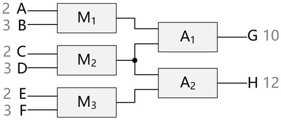
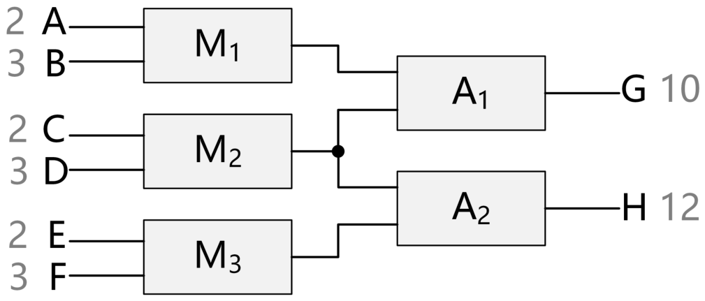
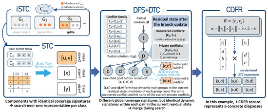
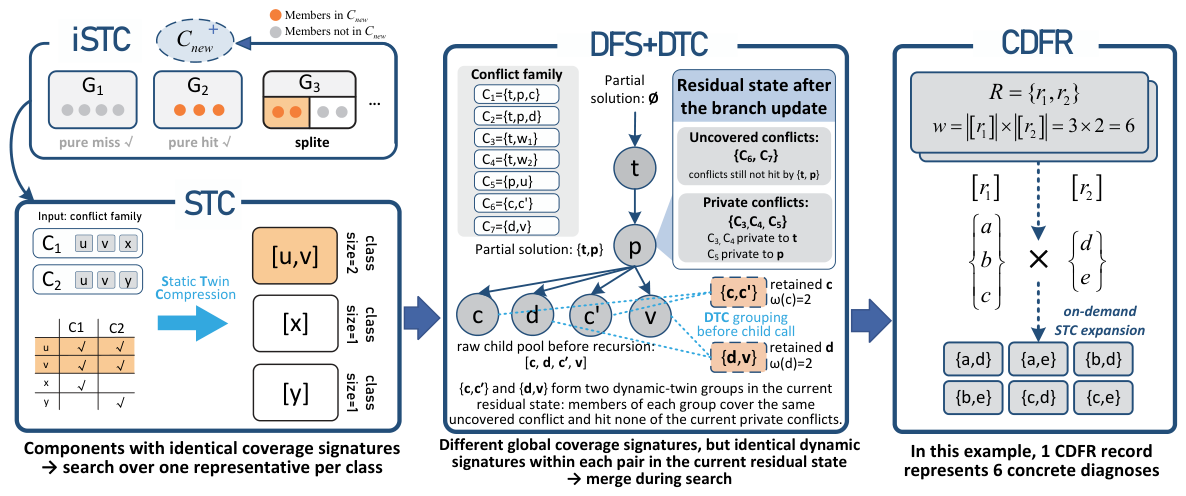
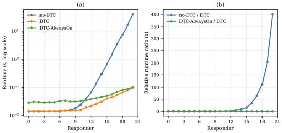
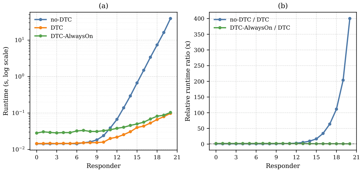

Disclaimer/Publisher’s Note: The statements, opinions and data contained in all publications are solely those of the individual author(s) and contributor(s) and not of MDPI and/or the editor(s). MDPI and/or the editor(s) disclaim responsibility for any injury to people or property resulting from any ideas, methods, instructions or products referred to in the content. |
© 2026 by the authors. Licensee MDPI, Basel, Switzerland. This article is an open access article distributed under the terms and conditions of the Creative Commons Attribution (CC BY) license.