


Abstract
With the steadily increasing penetration of renewable energy, the equivalent inertia of power systems continues to decline, and frequency stability is increasingly challenged. Consequently, a rapid and accurate assessment of the minimum inertia requirement is urgently needed. To address this challenge, this study proposes a mechanism–data fusion method for minimum inertia requirement assessment in renewable energy power systems. The assessment task is decomposed into two structurally symmetric subtasks corresponding to the mechanism and data pathways, where the same system operating state serves as the common input to both pathways. In the mechanism pathway, the minimum inertia requirement is analytically calculated using a generic system frequency response model with open-loop decoupling. In the data pathway, an extreme learning machine estimates the error between the mechanism result and the time-domain simulation benchmark to correct the mechanism result. Finally, the mechanism result and the data-based error compensation are summed to obtain the final assessment. Tests on the CSEE-FS power system show that the proposed method reduces the mean absolute percentage error from 9.33% to 0.23% and the root mean square error from 0.3957 s to 0.0114 s relative to the mechanism-only method. The average computation time is 0.16 s per operating condition, meeting the requirement for rapid online assessment.
1. Introduction
The growing penetration of renewable energy sources has led to a progressive decline in the equivalent inertia of power systems, making frequency stability an increasingly critical concern [1]. Under large disturbances, insufficient system inertia can cause an excessive rate of frequency decline and frequency deviation violations, potentially jeopardizing the secure operation of the power grid. Therefore, rapid and accurate assessment of the minimum inertia requirement is essential for maintaining system security and stability in renewable energy power systems [2,3].
In the assessment of minimum inertia requirements, detailed time-domain simulations can comprehensively capture system frequency dynamics and are therefore regarded as the most reliable benchmark [4]. However, under each operating condition, repeated simulations are required to determine the minimum inertia that satisfies the frequency constraint. This process provides accurate results but requires considerable computation time, making it difficult to use for online assessment. To reduce assessment time, simplified frequency stability models have been developed. According to the mechanism model used, existing methods can be divided into two categories: those based on the average system frequency (ASF) model and those based on the system frequency response (SFR) model.
The ASF model retains the speed-governing loop of each unit and therefore provides high analytical accuracy. However, complete analytical expressions of the governing systems are required, and the model order increases with the system size [5]. Based on the ASF model, reference [6] proposed an open-loop linear model that reduces the speed-governing systems of each generator to a first-order equivalent. This simplification reduces the model order and improves calculation efficiency. However, the first-order equivalent cannot fully represent the dynamic characteristics of the governing system, which reduces the accuracy of the frequency response calculation. To address this issue, references [7,8,9] developed a polynomial-fitting model for the governing systems. Nevertheless, the fitted model has limited generalizability and must be refitted when the operating condition changes. Furthermore, reference [10] proposed a generalized generator governing model that considers the different frequency response characteristics of different governor types. This model enables an analytical solution of the minimum inertia requirement with improved accuracy, but it also increases the model complexity and calculation time.
By contrast, the SFR model places a stronger emphasis on the rapidity of system frequency response analysis. The traditional SFR model typically comprises components such as equivalent inertia, an equivalent speed-governing system, and load damping. By applying equivalent simplifications to the system frequency dynamics, it captures the frequency response characteristics in a concise form, albeit with relatively low analytical accuracy [11]. To enhance the analytical accuracy of the SFR model, reference [12] proposed an analytical aggregation method for the multi-machine SFR model. This approach aggregates the governor parameters of individual units via normalized gain weighting, thereby reducing the multi-machine model to a single-machine equivalent and consequently improving computational precision. To account for the impact of renewable energy on frequency stability, references [13,14,15,16] incorporated renewable energy frequency regulation loops into the SFR model. These studies analyzed the underlying mechanisms and key factors by which renewable energy frequency regulation influences frequency stability and further evaluated the system’s minimum inertia requirement under renewable energy integration. Furthermore, to incorporate the impacts of diverse frequency regulation resources and improve the generalizability of the SFR model, references [17,18,19] proposed a generic SFR model. This model is tailored for dynamic frequency analysis of power grids integrating thermal, hydro, and renewable energy generation. It successfully simplifies the complexity of system frequency analysis while strictly preserving the distinct frequency regulation characteristics of different generator types.
Despite these advances, existing methods for minimum inertia requirement assessment still exhibit inherent limitations. Time-domain simulations accurately capture system dynamics but require considerable computation time. Simplified frequency analysis models reduce the calculation time, but the simplifications introduce errors in representing system frequency dynamics. These errors limit the accuracy of the minimum inertia requirement assessment.
To address these limitations, a symmetry-guided mechanism–data fusion method is proposed for assessing the minimum inertia requirement in renewable energy power systems. The assessment task is decomposed into two structurally symmetric subtasks corresponding to the mechanism and data pathways, where the same system operating state serves as the common input to both pathways. In the mechanism pathway, the minimum inertia requirement is analytically calculated using a generic system frequency response model with open-loop decoupling. In the data pathway, an extreme learning machine estimates the error between the mechanism result and the time-domain simulation benchmark to correct the mechanism result. Finally, the mechanism result and the data-based error compensation are summed to obtain the final assessment.
The remainder of this paper is organized as follows. Section 2 presents the mechanism-based analytical method for minimum inertia requirement assessment. Section 3 introduces the ELM-based error compensation method. Section 4 describes the implementation scheme of the proposed mechanism–data fusion method. Section 5 presents the case studies and evaluates the performance of the proposed method. Finally, Section 6 concludes the paper.
2. Analytical Assessment Method for Minimum Inertia Requirement Based on Mechanism Model
2.1. Generic SFR Model
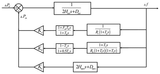
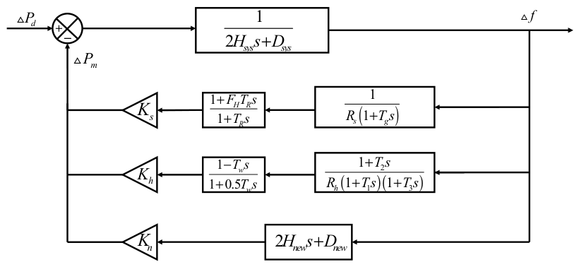
The generic SFR model [18,19] shown in Figure 1 is used as the mechanism model to derive the analytical solution of the minimum inertia requirement. Based on the center of inertia (COI) assumption, the system inertia is represented by a single equivalent inertia, and the frequency dynamics following a disturbance are described by the COI frequency. Unlike the classical SFR model, which uses a single equivalent governor, the generic SFR model retains separate speed-governing loops for thermal, hydro, and renewable energy units. It can therefore represent the different dynamic responses of these units and improve the accuracy of system frequency-response analysis.
Figure 1.
Generic SFR model.
In Figure 1, Hsys is the equivalent inertia constant of the system. Dsys is the system damping coefficient. ΔPd is the active power load disturbance. R is the droop coefficient. T1, T2, and T3 are the time constants of the corresponding speed-governing links. TW is the time constant of the water hammer effect for the hydro unit. TR is the reheat time constant of the thermal unit. FH is the high-pressure turbine power fraction. Ks, Kh, and Kn are the actual online capacities of thermal, hydro, and renewable energy units, respectively. Hnew is the virtual inertia of the renewable energy units. Dnew is the droop proportional gain coefficient of the renewable energy. Δf is the frequency deviation of the center of inertia, and s is the Laplace operator.
In this study, the minimum inertia requirement is defined as the lowest value of the system equivalent inertia constant Hsys that satisfies the frequency deviation limit under a given power disturbance.
2.2. Open-Loop Decoupling Simplification of the Generic SFR Model
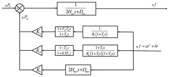
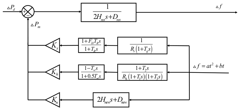
The generic SFR model provides an accurate representation of the system frequency response. However, its closed-loop structure makes it difficult to derive an analytical solution of the minimum inertia requirement. In the model, the frequency deviation Δf and the total primary frequency response power ΔPm are coupled, and their time-domain expressions cannot be derived separately. To obtain a rapid analytical solution, the speed-governing system is decoupled from the inertia-damping links. The frequency decline curve from the disturbance to the nadir is then approximated by a parabola [9]. As the frequency approaches the nadir, the magnitude of the rate of change in frequency decreases from its maximum value to zero. This trend is consistent with the derivative of a parabolic curve and provides the basis for the approximation. The resulting open-loop decoupled generic SFR model is shown in Figure 2.
Figure 2.
Open-loop decoupled generic SFR model.
2.3. Mechanism-Based Analytical Assessment Method for Minimum Inertia Requirement
The open-loop decoupled generic SFR model is used to derive the minimum inertia requirement of the system. Following a disturbance, the speed-governing systems gradually adjust the mechanical power output of the generator units to reduce the frequency deviation. Before the frequency reaches the nadir, the governor actuator remains unsaturated and opens at an approximately constant rate. During the initial stage of the frequency response, the mechanical power increment is assumed to increase linearly with time and reach its maximum value at the frequency nadir [9]. The linear approximation used in the subsequent derivation of the minimum inertia requirement is expressed as follows:
where ΔPd is the power deficit, tnadir is the time at which the frequency nadir occurs, and ΔPm is the mechanical power increment of the speed governing system.
The frequency response equation of the renewable energy-penetrated power system:
where ΔPm is the mechanical power variation, and ΔPe(t) is the electromagnetic power variation.
Substituting Equation (1) into Equation (2), and given that ΔPe(t) = ΔPd, we obtain the following equation:
Integrating Equation (3) with the initial condition Δf(0) = 0 gives the time-domain expression of Δf(t):
Taking the Laplace transform of Equation (4), we obtain the following:
According to the open-loop generic SFR model shown in Figure 2, the aggregate governor transfer function is expressed as
where Gh(s), Gs(s), and Gn(s) are the transfer functions of the hydro, thermal, and renewable energy units, respectively. According to the negative-feedback relationship shown in Figure 2, the mechanical power increment is given by
Applying the inverse Laplace transform to Equation (7) gives the time-domain mechanical power increment ΔPm(t). At the frequency nadir, the rate of change in frequency is zero. According to Equation (2) and ΔPe(t) = ΔPd, the following power-balance condition is obtained as follows:
Similarly, substituting the frequency nadir tnadir into Equation (4) yields
Equations (8) and (9) constitute a coupled nonlinear equation system with respect to tnadir and Hsys. Substituting Equation (9) into Equation (8) eliminates Hsys and gives
To obtain the explicit expression of Equation (10), the hydro and thermal governor transfer functions in Equation (6) are decomposed into first-order terms as follows:
where A1, A2, and A3 are the partial-fraction coefficients of the hydro governor, while B1 and B2 are those of the thermal governor.
After the inverse Laplace transformation of Equation (10), Equation (12) is obtained. Noted that at the frequency nadir, the rate of change in frequency is zero. Therefore, the virtual inertia term of the renewable energy component does not contribute at tnadir.
After giving the ΔPd and Δfnadir, all parameters in Equation (12) are known for a given operating condition, except tnadir. Therefore, Equation (12) is a one-dimensional nonlinear equation in tnadir. It is solved using the MATLAB R2024b built-in function fzero, which combines bisection, secant, and inverse quadratic interpolation. Candidate initial values of 1, 3, 5, 8, 10, 15, and 20 s are tested in sequence, and the admissible range of tnadir is set to 0.1–50 s. The default termination tolerance and iteration limit of fzero are used. A solution is accepted only when the solver converges successfully, and the obtained tnadir lies within the specified range. If the current initial value fails to produce a valid solution, the next candidate value is tested. If all candidate values fail, the operating condition is regarded as infeasible.
After tnadir is obtained, the minimum inertia requirement Hm corresponding to the given ΔPd and Δfnadir is calculated using
3. Data Method for Minimum Inertia Requirement Error Compensation
In the mechanism method, the speed-governing systems of the same type of units are aggregated, and open-loop decoupling is applied. These simplifications may cause differences between the mechanism calculation and the time-domain simulation result. To compensate for these differences, an ELM is used to learn the nonlinear relationship between the system operating state and the mechanism calculation error. The predicted error is then added to the mechanism result to obtain the final minimum inertia assessment.
3.1. Basic Principle of ELM
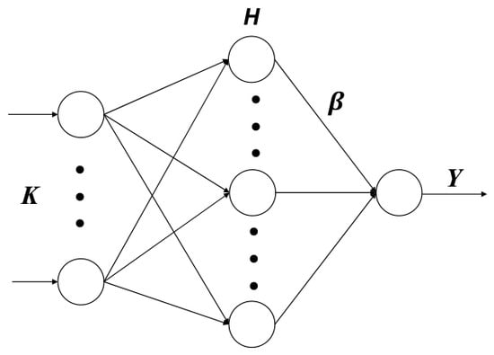
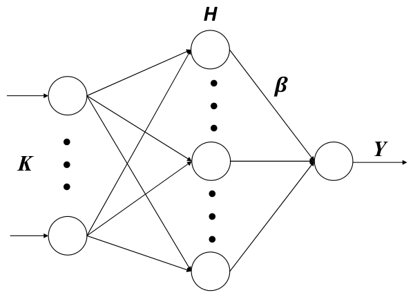
ELM is a single-hidden-layer feedforward neural network [20]. The input weights and hidden-layer biases are randomly initialized and remain fixed during training, while the output weights are obtained by solving a least-squares problem. The network structure is shown in Figure 3.
Figure 3.
Network structure diagram of ELM.
The ELM model can be expressed in matrix form as:
where H is the hidden layer output matrix, β is the output weight matrix, and Y is the target output matrix.
Since the input weights and hidden-layer biases remain fixed during training, the output weight matrix can be obtained by
where H† is the Moore–Penrose generalized inverse of H.
To further improve the generalization capability of the ELM, the output weights β can also be calculated as follows [20]:
where I denotes the identity matrix, and M is the regularization coefficient.
3.2. ELM-Based Error Compensation for Minimum Inertia Requirement
Because of the simplifications made in the mechanism model, its assessment result may differ from the time-domain simulation result. Let Hs denote the minimum inertia requirement obtained from time-domain simulation and Hm denote that calculated by the mechanism method. The error between them is defined as
Instead of directly predicting the minimum inertia requirement, the ELM is used to learn this error. The actual online capacities of thermal, hydro, and renewable energy units are selected as the input features. The input vector is expressed as
During training, K is used as the ELM input, and ΔH is used as the output label. For a given operating condition, the trained ELM provides the predicted error compensation value:
where ELM() denotes the nonlinear mapping learned by the ELM. The predicted value ΔHd is then used to correct the mechanism result.
4. Implementation Scheme of the Proposed Method
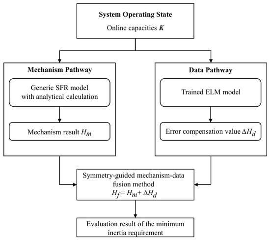
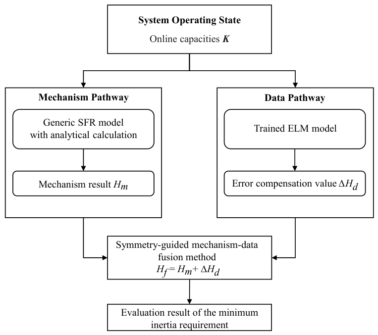
This section describes the implementation scheme for the proposed method for minimum-inertia requirement assessment, as shown in Figure 4. The implementation follows a structurally symmetric task decomposition: the same system operating state K, denoting the vector of online capacities of different generation units, serves as the common input to two independent yet complementary pathways.
Figure 4.
Implementation scheme of the proposed method.
In the mechanism pathway, the system operating state K is fed into the generic SFR model with open-loop decoupling, and the analytical solution of the minimum inertia requirement is obtained by Equation (13). The output of this pathway is the mechanism-based calculation Hm, which has a clear physical meaning and serves as the baseline for the final assessment.
In the data pathway, the same system operating state K is used as the input to the trained ELM model, as described in Equation (19). The output of this pathway is the data-based error compensation value ΔHd. This predicted value represents the data-driven correction that compensates for the errors in the mechanism pathway.
In the fusion step, Hm and ΔHd are summed as Hf = Hm + ΔHd to obtain the final assessment result of minimum inertia requirement.
5. Case Study
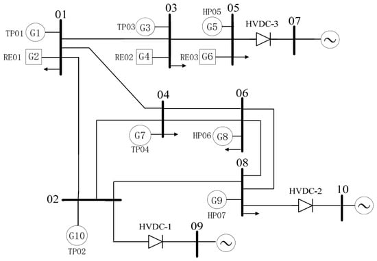
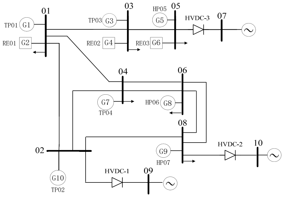
The proposed method is evaluated using the CSEE-FS standard test power system. Derived and simplified from a practical power grid, this system includes thermal, hydro, and renewable energy units. The installed capacities of these units are 2000, 3400, and 6900 MW, respectively. Figure 5 shows the single-line diagram of the system, and the remaining system parameters are provided in [21]. The experiments are performed using MATLAB/Simulink R2024b and Python 3.13. All experiments are executed on a computer equipped with an Intel Core i7-14650HX processor, 32 GB of RAM, and an NVIDIA GeForce RTX 5070 Ti Laptop GPU.
Figure 5.
Single-line diagram of CSEE-FS power system.
5.1. Data Generation
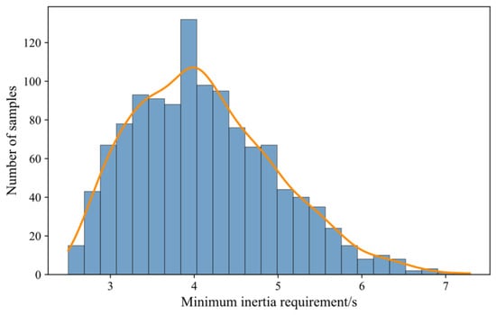
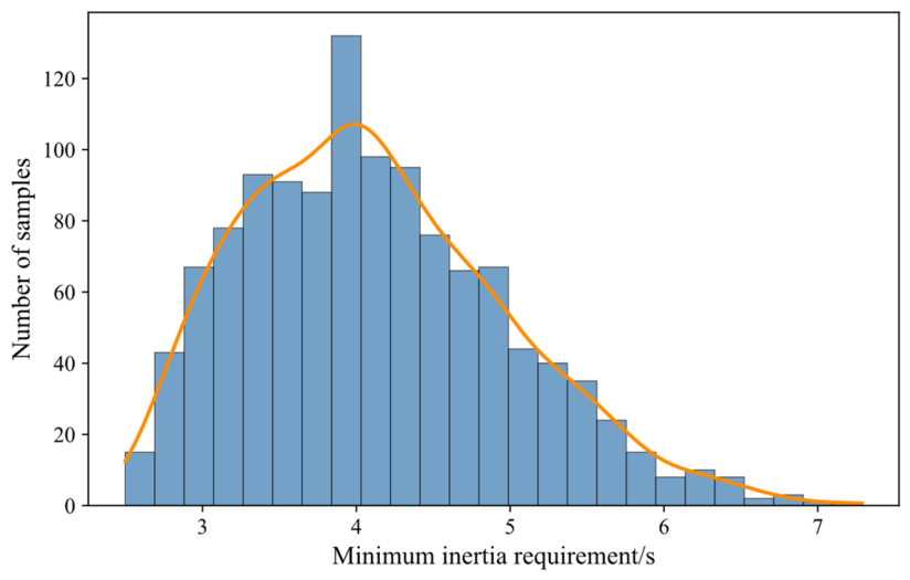
To generate sample data, the detailed parameters of the CSEE-FS system are first equivalenced into the generic SFR model. This model retains the main frequency response characteristics of hydro, thermal, and renewable energy units while simplifying the simulation modeling process, enabling accurate and efficient calculation of system frequency dynamics. Based on this model, the scaling factors of the three unit types are independently sampled from uniform distributions over 0.6–0.8, 0.7–0.9, and 0.5–0.8, respectively. A power disturbance of 1200 MW and a frequency deviation limit of 0.75 Hz are considered, and 1200 valid samples are obtained through time-domain simulation, with the mechanism-based analytical calculation results also derived for each operating condition. The distribution of the minimum inertia requirements in the generated dataset is shown in Figure 6.
Figure 6.
Distribution of minimum inertia requirement. The bars represent the number of samples in each interval, and the orange curve shows the smoothed distribution.
The 1200 samples are randomly divided into 960 training samples and 240 test samples, which are used for model development and final performance evaluation, respectively.
5.2. Performance Metrics
To evaluate the performance of the minimum-inertia requirement assessment methods, the mean absolute percentage error (MAPE), maximum absolute percentage error (MaxAPE), root mean square error (RMSE), and maximum absolute error (MaxAE) are used as the evaluation metrics. These metrics are defined as follows:
where Zt,i denotes the true value of the i-th sample, and Zp,i denotes the predicted value of the i-th sample.
5.3. The Performance Comparison of Error Compensation
To improve the error compensation performance of the ELM, a grid search with four-fold cross-validation is conducted to determine the number of hidden-layer neurons and the regularization coefficient. The input features and error labels are standardized using the Z-score method, and the sigmoid function is used as the hidden-layer activation function. The candidate numbers of hidden-layer neurons are 50, 100, 200, and 500, and the candidate regularization coefficients are 10−6, 10−4, 10−2, 10−1, 1, and 10. To reduce the influence of random initialization, each parameter combination is evaluated using 10 different random seeds, and the reported results are averaged over these 10 runs. The lowest mean validation RMSE is obtained with 200 hidden-layer neurons and a regularization coefficient of 10−4, resulting in a 3–200–1 network structure. This parameter setting is used in the subsequent experiments.
To compare the error compensation performance of the ELM with other machine learning models, support vector regression (SVR) [22], multilayer perceptron (MLP) [23], and random forest (RF) [24] were selected as the benchmark models. The SVR model used a radial basis function kernel with a penalty coefficient of 1.0. The MLP model consisted of one hidden layer with 100 neurons and was trained using the Adam optimizer. The RF model consisted of 100 regression trees and used the squared-error criterion. The comparison results are shown in Table 1.
Table 1.
Error compensation performance of different models.
As shown in Table 1, the ELM achieves the lowest MAPE, RMSE, and MaxAE among the four models, with values of 2.48%, 0.0114 s, and 0.0351 s, respectively. The MLP achieves the lowest MaxAPE of 11.02%, while the MaxAPE of the ELM is 14.08%. Although the ELM does not achieve the lowest MaxAPE, it performs best across the other three metrics and provides better overall error compensation performance.
5.4. Result Analysis of the Mechanism-Data Fusion Method
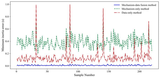
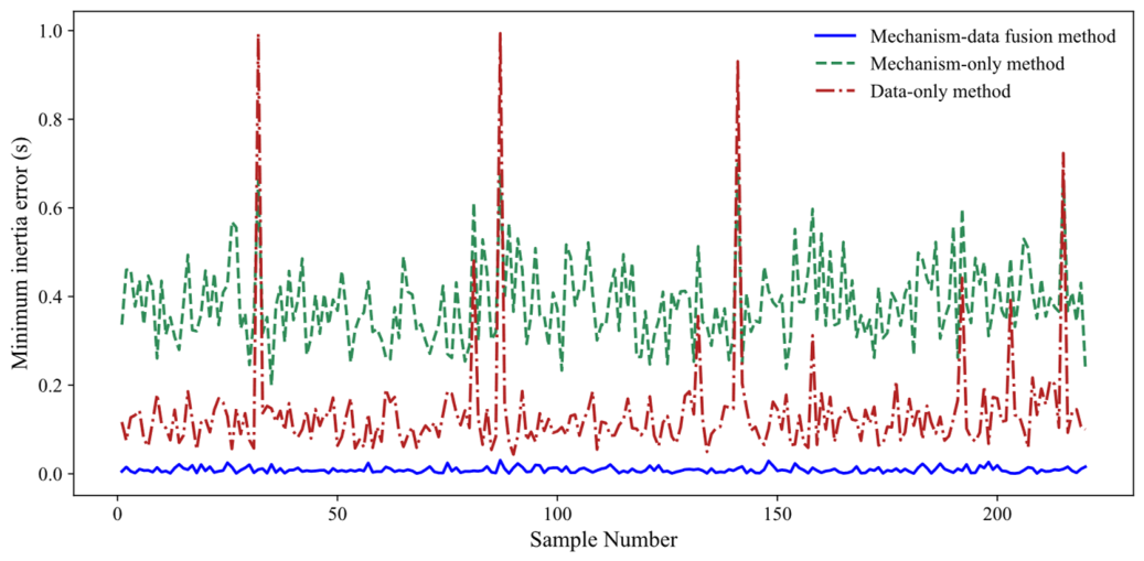
The assessment performance is evaluated on the test set by comparing three methods: the mechanism-only, the data-only, and the proposed fusion method. In the data-only method, the ELM directly predicts the complete minimum inertia requirement without any physical guidance. Figure 7 compares the sample-wise assessment errors of the three methods. The data-only method produces relatively large errors for some samples due to the lack of a physical basis, whereas the proposed fusion method achieves lower errors than the other two methods for all test samples.
Figure 7.
Comparison of sample minimum inertia estimation errors among different methods.
The performance metrics of the three methods are presented in Table 2, including MAPE, MaxAPE, RMSE, and MaxAE. As shown in Table 2, the data-only method achieves lower MAPE and RMSE than the mechanism-only method. However, its MaxAPE and MaxAE are higher, indicating that relatively large errors remain in some samples. In contrast, the proposed mechanism–data fusion method achieves the lowest values for all four metrics on the independent test set, with MAPE, MaxAPE, RMSE, and MaxAE of 0.23%, 1.06%, 0.0114 s, and 0.0351 s, respectively. These results demonstrate that the proposed method improves overall accuracy and effectively reduces large errors in challenging samples.
Table 2.
Comparison of error results for different methods.
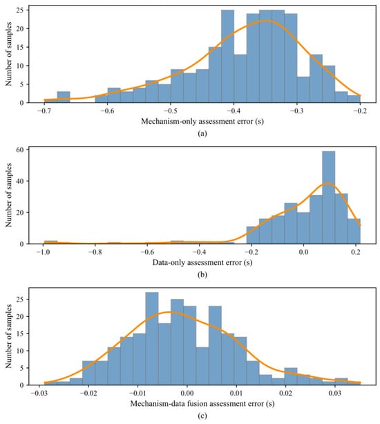
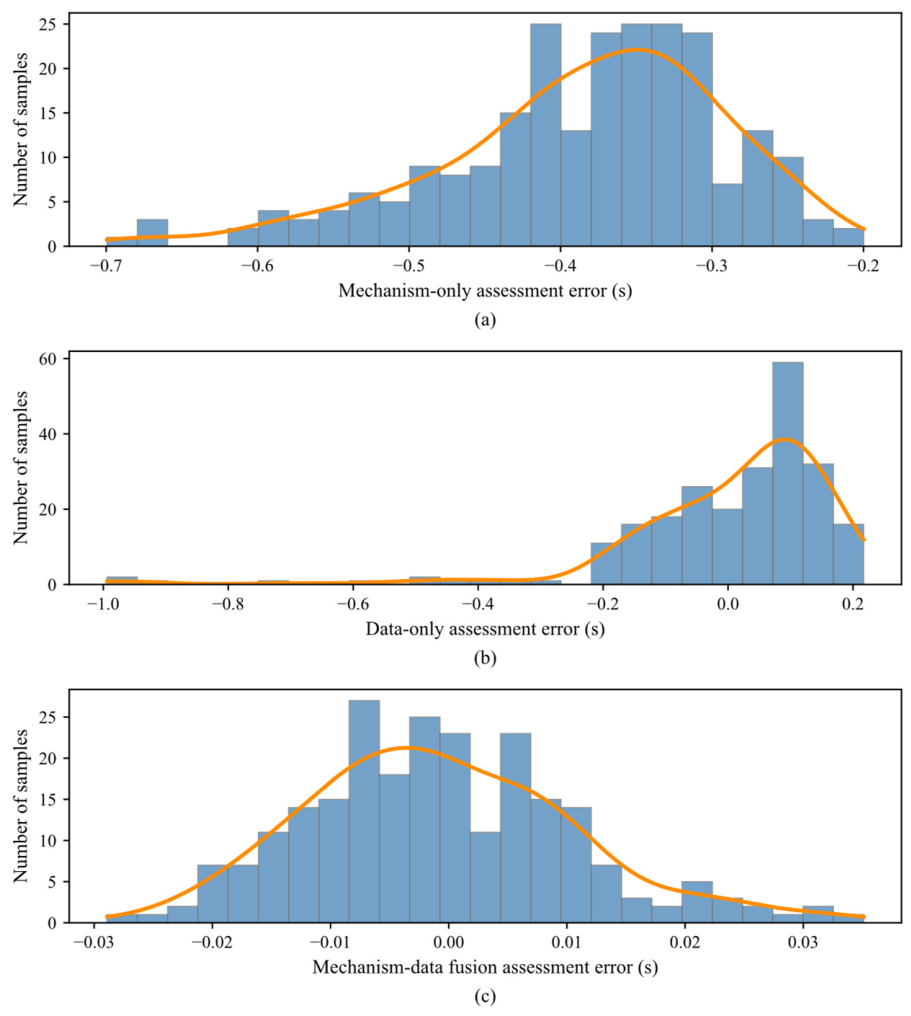
Furthermore, Figure 8 presents the error distributions of the three methods on the independent test set. The mechanism-only method exhibits a clear systematic bias, with errors distributed relatively far from zero. The data-only method reduces the overall bias, though several samples still show relatively large errors. In contrast, the proposed method yields errors tightly concentrated around zero, with the narrowest distribution among the three methods. These results confirm that the data compensation effectively corrects the systematic bias of the mechanism calculation and improves agreement with the time-domain simulation benchmarks.
Figure 8.
Error distributions of minimum inertia assessment under different methods: (a) Mechanism-only method; (b) data-only method; (c) mechanism-data fusion method. The bars represent the number of samples in each error interval, and the orange curves show the smoothed error distributions.
5.5. Effect of Training Sample Size on Method Performance
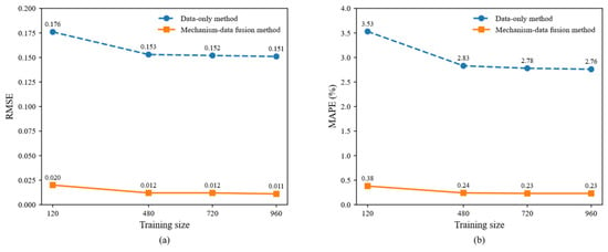
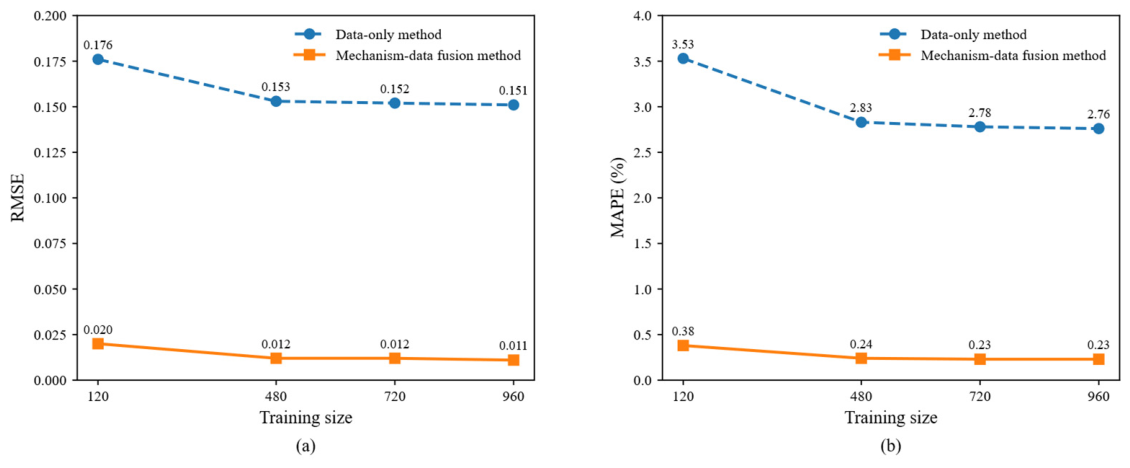
Figure 9 shows the effect of the training sample size on the RMSE and MAPE of the data-only and proposed mechanism–data fusion methods. When the training sample size increases from 120 to 480, for the data-only method, the RMSE decreases from 0.176 s to 0.153 s and the MAPE from 3.53% to 2.83%, while for the proposed method, the RMSE decreases from 0.020 s to 0.012 s and the MAPE from 0.38% to 0.24%. The proposed method exhibits a more gradual decline over the same sample size increment, suggesting lower sensitivity to additional training data. When the sample size exceeds 480, the RMSE of both methods remains nearly unchanged, whereas the MAPE of the data-only method continues to improve with increasing sample size, while that of the proposed method remains essentially stable. These observations indicate that the proposed mechanism–data fusion method, benefiting from its physical basis, achieves better performance with fewer training samples compared to the data-only method.
Figure 9.
Effect of training sample size on model performance: (a) RMSE comparison; (b) MAPE comparison.
5.6. Computation Time Analysis
To evaluate the rapid assessment capability of the proposed method, the computation times of different methods are compared on the test set. The results are summarized in Table 3.
Table 3.
Computation time of different methods.
As shown in Table 3, the time-domain simulation requires 3057.60 s for the entire test set, with an average of 12.74 s per sample. The mechanism-only method requires 37.97 s in total and 0.16 s per sample. Adding the data compensation model increases the total computation time by only approximately 10−4 s. Therefore, the total and average computation times of the proposed method remain 37.97 s and 0.16 s, respectively. This is only 1.24% of the time required by the time-domain simulation. These results show that the proposed method meets the requirement for rapid online assessment of the minimum inertia requirement.
6. Conclusions
To meet the requirement of rapid and accurate assessment of minimum inertia in renewable energy power systems, a symmetry-guided mechanism–data fusion method is proposed. A generic SFR model is used to represent the different frequency responses of thermal, hydro, and renewable energy units. Open-loop decoupling is then applied to obtain a rapid analytical solution of the minimum inertia requirement. To correct the resulting mechanism calculation error, an ELM-based data compensation model is established using the actual online capacities of the three types of units as inputs. The predicted error is added to the mechanism result to obtain the final assessment. Case studies show that the proposed method improves assessment accuracy while meeting the requirement for rapid online calculation.
Future work will focus on developing more reliable fusion mechanisms and methods at the mechanism-data interface, including adaptive weighting schemes and credibility-based fusion strategies, to further improve the trustworthiness of the fused results.
Author Contributions
Conceptualization, Y.Z. and X.D.; methodology, F.L.; software, Y.M.; validation, J.Y., X.D. and Y.Z.; formal analysis, Y.M.; investigation, Y.Z.; resources, X.D.; data curation, F.L.; writing—original draft preparation, Y.M.; writing—review and editing, J.Y.; visualization, Y.Z.; supervision, X.D.; project administration, F.L.; funding acquisition, X.D. All authors have read and agreed to the published version of the manuscript.
Funding
This work was supported by the Science and Technology Project of State Grid Sichuan Electric Power Company, “Research on Key Technologies for Friendly Grid Connection Support of New Energy Bases in Western Sichuan” (No. 521996250006).
Data Availability Statement
The original contributions presented in this study are included in the article. Further inquiries can be directed to the corresponding author.
Acknowledgments
The authors would like to acknowledge the support provided by the State Grid Sichuan Electric Power Company.
Conflicts of Interest
Authors Yongjie Zhang, Xinwei Du, and Fang Liu were employed by the State Grid Sichuan Economic Research Institute. The authors declare that this study received funding from the Science and Technology Project of State Grid Sichuan Electric Power Company “Research on Key Technologies for Friendly Grid Connection Support of New Energy Bases in Western Sichuan” (No.521996250006). The funder had the following involvement with the study: research design, methodology development, data curation, formal analysis, investigation, supervision, project administration, and writing.
References
- Fernandez-Bernal, F.; Egido, I.; Lobato, E. Maximum wind power generation in a power system imposed by system inertia and primary reserve requirements. Wind Energy 2015, 18, 1501–1514. [Google Scholar] [CrossRef] [Scilit]
- Kou, G.; Markham, P.N.; Hadley, S.; King, T.; Liu, Y. Impact of governor deadband on frequency response of the U.S. Eastern interconnection. IEEE Trans. Smart Grid 2016, 7, 1368–1377. [Google Scholar] [CrossRef] [Scilit]
- Baek, B.; Shin, H. Time-based technical requirements for fast frequency response robust across inertia levels. IEEE Access 2026, 14, 16010–16021. [Google Scholar] [CrossRef] [Scilit]
- Gu, H.; Yan, R.; Saha, T.K. Minimum synchronous inertia requirement of renewable power systems. IEEE Trans. Power Syst. 2018, 33, 1533–1543. [Google Scholar] [CrossRef] [Scilit]
- Chan, M.L.; Dunlop, R.D.; Schweppe, F. Dynamic equivalents for average system frequency behavior following major disturbances. IEEE Trans. Power Appar. Syst. 1972, PAS-91, 1637–1642. [Google Scholar] [CrossRef] [Scilit]
- Egido, I.; Fernandez-Bernal, F.; Centeno, P.; Rouco, L. Maximum frequency deviation calculation in small isolated power systems. IEEE Trans. Power Syst. 2009, 24, 1731–1738. [Google Scholar] [CrossRef] [Scilit]
- Jung, J.; Park, J.; Choi, J.H.; Lee, G.S. An analytic method for frequency nadir estimation in fast frequency response resource (FFRR) dominant power systems. IEEE Trans. Power Deliv. 2026, 41, 1337–1349. [Google Scholar] [CrossRef] [Scilit]
- Zhao, Z.; Xue, Y.; Chu, Z.; Guo, Y.; Li, Z.; Lin, S.; He, X.; Teng, F.; Strbac, G. Generic low-order primary frequency response model for frequency nadir prediction. IEEE Trans. Power Syst. 2025, 40, 5221–5236. [Google Scholar] [CrossRef] [Scilit]
- Liu, L.; Li, W.; Ba, Y.; Shen, J.; Jin, C.; Wen, K. An analytical model for frequency nadir prediction following a major disturbance. IEEE Trans. Power Syst. 2020, 35, 2527–2536. [Google Scholar] [CrossRef] [Scilit]
- Peng, Z.; Peng, Q.; Zhang, Y.; Han, H.; Yin, Y.; Liu, T. Online inertia allocation for grid-connected renewable energy systems based on generic ASF model under frequency nadir constraint. IEEE Trans. Power Syst. 2024, 39, 1615–1627. [Google Scholar] [CrossRef] [Scilit]
- Anderson, P.M.; Mirheydar, M. A low-order system frequency response model. IEEE Trans. Power Syst. 1990, 5, 720–729. [Google Scholar] [CrossRef] [Scilit]
- Shi, Q.; Li, F.; Cui, H. Analytical method to aggregate multi-machine SFR model with applications in power system dynamic studies. IEEE Trans. Power Syst. 2018, 33, 6355–6367. [Google Scholar] [CrossRef] [Scilit]
- Hamanah, W.M.; Shafiullah, M.; Alhems, L.M.; Alam, M.S.; Abido, M.A. Realization of robust frequency stability in low-inertia islanded microgrids with optimized virtual inertia control. IEEE Access 2024, 12, 58208–58221. [Google Scholar] [CrossRef] [Scilit]
- Xia, Y.; Wang, Q.; Miao, C.; Tang, Y. An extended SFR model based fast frequency security assessment method for power systems. Energy Rep. 2023, 9, 2045–2053. [Google Scholar] [CrossRef] [Scilit]
- Dhara, P.K.; Rather, Z.H.; Phurailatpam, C. Estimation of minimum inertia and fast frequency support for renewable energy dominated power systems. IEEE Trans. Instrum. Meas. 2025, 74, 9001114. [Google Scholar] [CrossRef] [Scilit]
- Krpan, M.; Kuzle, I. Introducing low-order system frequency response modelling of a future power system with high penetration of wind power plants with frequency support capabilities. IET Renew. Power Gener. 2018, 12, 1453–1461. [Google Scholar] [CrossRef] [Scilit]
- Ju, P.; Zheng, Y.; Jin, Y.; Qin, C.; Jiang, Y.; Cao, L. Analytic assessment of the power system frequency security. IET Gener. Transm. Distrib. 2021, 15, 2215–2225. [Google Scholar] [CrossRef] [Scilit]
- Huang, H.; Ju, P.; Jin, Y.; Yuan, X.; Qin, C.; Pan, X.; Zang, X. Generic system frequency response model for power grids with different generations. IEEE Access 2020, 8, 14314–14321. [Google Scholar] [CrossRef] [Scilit]
- Ding, Q.; Zhang, X.; Li, Z.; Wang, X.; Li, W. Fast assessment method for minimum demand inertia in power systems. J. Mod. Power Syst. Clean Energy 2026, 14, 95–107. [Google Scholar] [CrossRef] [Scilit]
- Huang, G.B.; Zhou, H.; Ding, X.; Zhang, R. Extreme learning machine for regression and multiclass classification. IEEE Trans. Syst. Man Cybern. B Cybern. 2012, 42, 513–529. [Google Scholar] [CrossRef] [Scilit] [PubMed]
- Sun, H.; Zhao, B.; Xu, S.; Lan, T.; Li, Z.; Wu, P. Test models for stability/security studies of AC-DC hybrid power systems with high penetration of renewables. IEEE Trans. Power Syst. 2025, 40, 957–969. [Google Scholar] [CrossRef] [Scilit]
- Cortes, C.; Vapnik, V. Support-vector networks. Mach. Learn. 1995, 20, 273–297. [Google Scholar] [CrossRef] [Scilit]
- Murtagh, F. Multilayer perceptrons for classification and regression. Neurocomputing 1991, 2, 183–197. [Google Scholar] [CrossRef] [Scilit]
- Breiman, L. Random forests. Mach. Learn. 2001, 45, 5–32. [Google Scholar] [CrossRef] [Scilit]

Disclaimer/Publisher’s Note: The statements, opinions and data contained in all publications are solely those of the individual author(s) and contributor(s) and not of MDPI and/or the editor(s). MDPI and/or the editor(s) disclaim responsibility for any injury to people or property resulting from any ideas, methods, instructions or products referred to in the content. |
© 2026 by the authors. Licensee MDPI, Basel, Switzerland. This article is an open access article distributed under the terms and conditions of the Creative Commons Attribution (CC BY) license.