Improving Electrical-Impedance-Tomography Reconstruction Quality by Sensitivity Matrix Transformation Using Diagonal Matrices

Abstract

As an advanced visualization technique, electrical impedance tomography (EIT) can reconstruct the distribution of electrical parameters and thereby visually show object distribution within a detection field. The quality of EIT reconstruction greatly depends on a selected sensitivity matrix, while various matrices can lead to very different EIT reconstruction results. A large number of efforts to improve the sensitivity matrix have been made to enhance EIT reconstruction quality, but how to construct and select a better matrix in a general and feasible way remains unsolved to date. In this paper, we use the matrix transformation method to address the issue, and two types of symmetric and diagonally dominant matrices are optimally selected to multiply the sensitivity matrix on the left and right, respectively. Therefore, EIT reconstruction quality can generally be improved. The feasibility and robustness of the proposed method have been theoretically demonstrated for both Gaussian kernel-based and power function-based matrices. Experiments validate the proposed method by EIT reconstruction quality.

1. Introduction

Electrical impedance tomography (EIT) [1] can reconstruct the distribution of electrical parameters and thereby visually show the distribution of the object within a detection field. EIT has increasingly been used in most application fields [2,3,4,5]. However, the reconstruction quality of EIT is constrained by its inherent ill-posedness and soft-field effects [6,7]. In the past decades, developing high-quality EIT reconstruction algorithms has been a research focus.

EIT reconstruction quality depends on the selected algorithm and the available measurements. Existing EIT algorithms include direct and indirect types [8]. The direct methods include linear back-projection (LBP) [9], algebraic computation [10], D-bar [11], and others. The indirect methods usually rely on optimization techniques and related prior parameters, such as conjugate gradient (CG) [12], Tikhonov regularization (TR) [13], and the Landweber iteration (LW) [14]. However, EIT reconstruction quality depends heavily on the selected sensitivity matrix, and different matrices can yield very different results [15]. To improve EIT reconstruction quality, various EIT algorithms use different matrix transformations on the left or right side of the original sensitivity matrix as follows.

(1) Left multiplication of a matrix. A typical example is the modified LBP algorithm, which multiplies the sensitivity matrix on the left by a filter matrix. The one-step TR algorithm multiplies an invertible matrix on the left of the sensitivity matrix, while Ding et al. [16] described a nonlinear second-order sensitivity matrix and added one nonlinear term on the left of the sensitivity matrix. Liu et al. [17] began with the perspective of compressed sensing and represented the distribution of electrical parameters using a Fourier basis and reconstructed the sensitivity matrix. Generally, almost all EIT methods need to normalize a sensitivity matrix, which naturally multiplies the corresponding transformation matrix by the existing sensitivity matrix on the left [18].

Recently, Yue et al. [19] demonstrated that most existing EIT algorithms have a unified form, and their differences result from multiplying different transformation matrices by the existing sensitivity matrix on the left. Therefore, the left multiplication of a selected matrix to the existing sensitivity matrix has become a useful way to improve EIT reconstruction quality.

(2) Right multiplication by a matrix. Moura et al. [20] proposed a sparse reconstruction scheme using a redundant sensitivity matrix. The scheme utilized K-singular value decomposition and nonlinear simulation to develop a dictionary learning model with real data. Dong et al. [21] used a nonlinear symmetric matrix to multiply the existing sensitivity matrix on the right, and the new sensitivity matrix not only addresses the limitations of the existing one but also is easily realized and controlled in practice via a kernel-width parameter. Barber et al. [22] originally proposed a filtering LBP algorithm that selects an additional matrix to improve the sensitivity matrix.

The above advancements are credited to using the matrix transformation on the existing sensitivity matrix. However, given a set of EIT measurements, determining the best matrix for the existing sensitivity matrix on the left or right remains unsolved to date and lacks theoretical and practical guidelines. To address the issue, in this paper, we first demonstrate that left- and right-multiplying an existing sensitivity matrix by a selected diagonal matrix can reduce its condition number, thereby increasing the feasibility and robustness of the EIT reconstruction results in the mathematical sense. Then, two types of transformation matrices, the Gaussian kernel and the power function, are introduced to improve EIT reconstruction quality and the robustness of the solution. Typical simulations have verified the feasibility and robustness of our proposed method.

2. Related Work

This section introduces the ERT principle, then presents three typical EIT algorithms used to validate the proposed methodology in this study, and finally introduces two works on right multiplication for a sensitivity matrix.

2.1. EIT Principle

The EIT techniques mainly include electrical resistance tomography (ERT) [23], electrical capacitance tomography (ECT) [24], and electrical magnetic tomography (EMT) [25], all of which have similar mathematical expressions. Thus, we only emphasize ERT as an example to explain the EIT principle as follows.

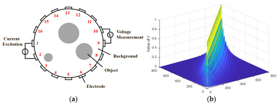
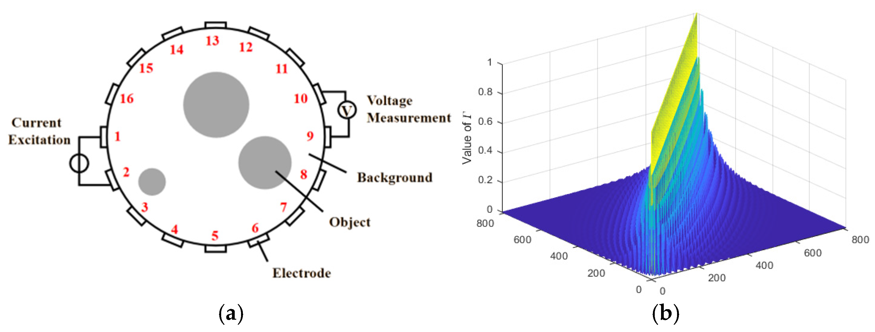
Let Ω represent a circular ERT detection field bounded by ∂Ω, to which m measurement electrodes are attached to reconstruct an ERT image, as shown in Figure 1a.

Figure 1. (a) ERT measuring principle; (b) a symmetric and diagonally dominant matrix κ.

We used a typical 16-electrode ERT system with an adjacent-excitation and adjacent-measurement way, and 208 measurements were obtained [26]. Partition Ω into n units (pixels) in which σ is the normalized conductivity vector, σ = (σ₁, σ₂, …, σ_n)^T. ERT aims at determining the conductivity distributions of n units based on all measurements on ∂Ω: u₁, u₂, …, u₂₀₈, denoting the measurement vector as U = (u₁, u₂, …, u₂₀₈)^T. Based on the finite element method [27], the linearized relationship from σ to U can nearly be expressed as

U = Sσ, s.t., U ∈ ∂Ω, σ ∈ Ω

(1)

where S is called the sensitivity matrix in the ERT imaging process; S = {s_ij} ∈ R^240×n, which reflects a linear map of unit (pixel) from σ to U. To solve σ along with U, S is usually determined in advance.

2.2. EIT Algorithms

The direct and easily realized EIT algorithm is linear back-projection (LBP), which is solved by

σ = S^TU, s.t., U ∈ ∂Ω, σ ∈ Ω

(2)

where S^T is the transpose matrix of S.

Furthermore, the issue of solving the variable σ in (1) is turned to optimize the following objective function:

min z = ‖Sσ − U‖

(3)

where ‖ · ‖ is a specified norm. The LW algorithm [28] is a typical iteration solution and is formulated as

$${\sigma }_{k+1}={\sigma }_k-\omega S^T(S{\sigma }_k-U),\hspace{0.33em}k=1,\hspace{0.33em}2,\hspace{0.33em}\dots$$

(4)

where 0 ≤ ω ≤ 2/‖S‖. The LW algorithm can converge quickly and is nonparametric.

The TR algorithm is another frequently used EIT algorithm for dealing with the ill-posed problem by a regularization process, which solves σ by optimizing the objective function as

$${\min }_{\sigma }\hspace{0.33em}z=\{\Vert U-S\sigma \Vert +\lambda R(\sigma )\}$$

(5)

where the regularization item R(σ) is often taken as ‖σ‖² to obtain an analytical solution (S^TS + λI)⁻¹S^T, which actually left-multiplies a matrix (S^TS + λI)⁻¹ to the transpose of S. The λ in TR is a hyperparameter, and its different values may greatly affect the imaging quality. The L-curve method [29] is often used to select the optimal parameter λ.

The ARW algorithm expands the exponent of the regularization term to (0, 2], which can greatly enhance solution sparsity and improve model robustness [30].

The objective function with the L_p norm can be expressed as

$$\min \hspace{0.33em}z=\{\Vert U-S\sigma {\Vert }_2^2+\lambda \Vert \sigma {\Vert }_p^p\}$$

(6)

And σ can be solved by the following iteration:

$${\sigma }_{k+1}={(S^{T}S+\lambda D)}^{-1}{S}^{T}U$$

(7)

where D is defined as

$$D=p|{\sigma }_k{|}^{p-2}/2$$

(8)

The calculation steps of the algorithm are as follows:

(1)

Initialize D = I, t = 0;

(2)

Update σ by (7);

(3)

Calculate the diagonal matrix D by (8), where the ith diagonal element is d_i = p/2|σ_i|^p−2;

(4)

t = t + 1; if t = T, stop. Otherwise, return to (2).

In the ARW algorithm, the results obtained from the previous iteration are incorporated as prior information into the computation of the next iteration, thereby enhancing the quality of the reconstructed image.

The previous study, Ref. [19] concluded that most of the existing EIT algorithms can be generally formulated as

σ = M(S)U, s.t., U ∈ ∂Ω, σ ∈ Ω

(9)

where M(•) stands for various matrices along different EIT algorithms and M(S) = {f(s_ij)}, where f(s_ij) is the computed sensitivity coefficients, i = 1, 2, …, m; j = 1, 2, …, n.

2.3. Right Multiplication for a Sensitivity Matrix

Compared with left multiplication, few studies focus on right multiplication for a sensitivity matrix. However, there are two remarkable advancements. One uses the following Gaussian kernel function to compute the distance between any pair of units (pixels), $R$ and $R^{\prime }$, in Ω [21,31]:

$$g(R,R^{\prime })=e^{-\Vert R-R^{\prime }\Vert /(2{\Gamma }^2)}$$

(10)

where Γ is the kernel width of the function. After denoting G = {g(R, R′)}, it updates S by S′, i.e.:

$$S^{\prime }=SG,\hspace{0.33em}s.t.,\hspace{0.17em}S,S^{\prime }\in R^{m\times n},\hspace{0.33em}G=\{\sigma (R_i,R_i^{\prime })\}\in R^{n\times n}$$

(11)

Therefore, (1) is turned to solve the equation S′σ = U. When G is a diagonally dominant matrix, as shown in Figure 1b, the reconstruction quality based on S′ has been demonstrated to be higher than that based on S.

The other is the filtered back-projection (FBP) algorithm [22]. According to the filtering principle for all measurements, FBP reconstructs any EIT image by

$$\sigma =B{(SB)}^{-1}U, s.t., U\in \partial \Omega , \sigma \in \Omega$$

(12)

The equation shows that FBP firstly multiplies a selected matrix B on the right of S to filter all measurements U. Then, these filtered data are then back-projected to form the image σ.

However, there are at least three problems. First, when a group of EIT measurements is available, how to select the better matrix for S remains unsolved to date. Second, why the Gaussian kernel improves imaging quality remains unclear, as there are no theoretical or practical guidelines. Finally, it is unclear whether the left and right multiplications can both improve EIT reconstruction. In this paper, we first demonstrate that multiplying matrix S on the left and right by diagonal matrices can reduce its condition number and thus improve reconstruction quality. Then, under the basic form of the matrix, we improve the form of the right-hand matrix of S by introducing two typical kernel matrices, such as the Gaussian kernel and the power function. Finally, the optimization and generalization of our proposed method are verified using the two kernel matrices through typical experiments.

3. EIT Reconstruction by Matrix Transformation

In this section, we first discuss the theoretical and practical meanings of multiplying the sensitivity matrix S by a pair of diagonal matrices. Then, the two symmetric and diagonally dominant matrices are used to improve the quality of EIT reconstruction.

3.1. The Meaning of Multiplying a Diagonal Matrix to S

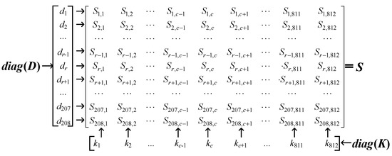
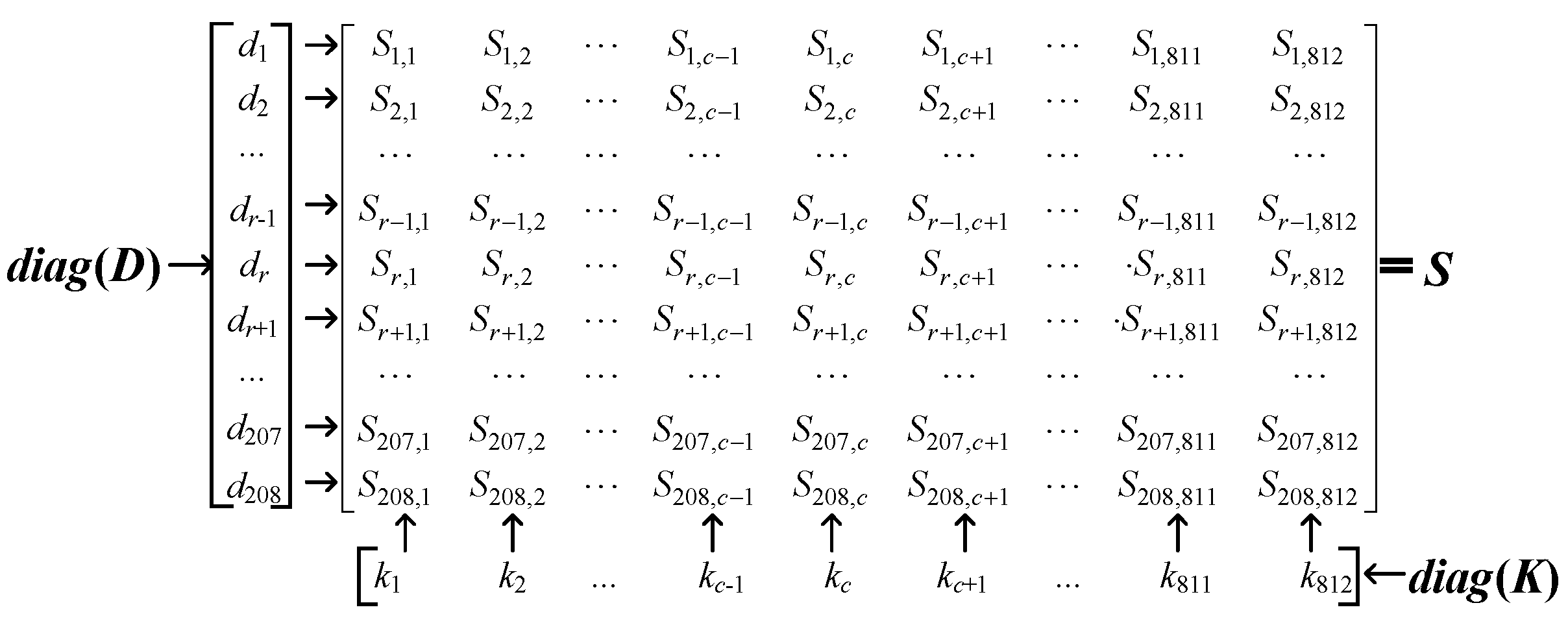
Let Ω be a detection field, which is typically discretized into 812 pixels for the 208 measurements acquired from 16 electrodes. Multiplying two diagonal matrices by the sensitive matrix S on the left and right refers to performing transformations on the columns and rows of S, as shown in Figure 2, where D₁ = diag{d₁, d₂, …, d₂₀₈} and D₂ = diag{k₁, k₂, …, k₈₁₂}.

Figure 2. Illustration of left and right multiplications of S.

When D₁ and D₂ are multiplied to S on the left and right, the matrix transformations have clear practical and theoretical meanings. Let $S={[{\overrightarrow{p}}_1,{\overrightarrow{p}}_2,\dots ,{\overrightarrow{p}}_{208}]}^T=[{\overrightarrow{q}}_1,{\overrightarrow{q}}_2,\hspace{0.33em}\dots \hspace{0.33em},\hspace{0.17em}{\overrightarrow{q}}_{812}]$, where ${\overrightarrow{p}}_s$ and ${\overline{q}}_t$ are the row vector and the column vector of S, respectively. The effects of both D₁ and D₂ are explained as follows.

(1)

Practical meanings. Note that

$$\left\{\begin{array}{l}{D}_{1}S={[d_1{\overrightarrow{p}}_1,\hspace{0.33em}{d}_2{\overrightarrow{p}}_2,\dots ,\hspace{0.17em}{d}_{208}{\overrightarrow{p}}_{208}]}^T\\ S{D}_2=[c_1{\overrightarrow{q}}_1,\hspace{0.33em}\hspace{0.17em}{c}_2{\overrightarrow{q}}_2,\dots ,\hspace{0.17em}{c}_{812}{\overrightarrow{q}}_{812}]\end{array}\right.$$

(13)

Since ${\overrightarrow{p}}_s$ points to the sth measurement, d₁ determines the degree of importance of the measurement. It was verified in [32] that various measurements have different signal-to-noise ratios, and thus have different effects when reconstructing any EIT image. Alternatively, ${\overline{q}}_t$ can endow various weights to different pixels to place stress on these interesting objects.

(2)

Theoretical meanings. Using these matrix transformations, the condition number of S can be reduced. We use the matrix balancing theory [33] for solving (1), and thereby achieve more effective solutions, as explained below.

Let the two diagonal matrices D₁ and D₂ multiply S individually on the left and right, and obtain an equivalent equation that has the same solution as (1) as follows:

(D₁SD₂) σ = D₁U, s.t., U ∈ ∂Ω, σ ∈ Ω

(14)

where D₁ is constructed based on the following steps:

(1)

Calculate the norm of each row (commonly L₂-norm or L_∞-norm): s_i = ‖S_i·‖, i = 1, 2, …, m, where “S_i·” refers to the norm for each row vector in S;

(2)

Avoid the zero norm: if s_i = 0, d_i = 1; otherwise, d_i = 1/s_i;

(3)

Generate the diagonal matrix:

D₁ = diag{d₁, d₂, …, d_m} ∈ R^m×m

(15)

Then, the diagonal matrix D₂ is constructed as follows:

(1)

Calculate the norm of each column (commonly L₂-norm or L_∞-norm): t_j = ‖S_·j‖, j = 1, 2, …, n, where “S_·j” refers to the norm for each column vector in S);

(2)

Avoid the zero norm: if t_i = 0, c_i = 1; otherwise, c_i = 1/t_i;

(3)

Generate the diagonal matrix:

D₂ = diag{c₁, c₂, …, c_n} ∈ R^n×n

(16)

where both D₁ and D₂ must be normalized by dividing their maximum value to decrease the condition number of S.

Based on the obtained D₁ and D₂ values, (1) is turned to

AY = B, s.t., A = D₁SD₂; Y = σ; B = D₁U

(17)

Consequently, σ is solved by (17).

The theoretical basis of using D₁ and D₂ to reduce the conditional number of S is illustrated as follows.

Lemma 1.

When B and A satisfy (17) based on D₁ and D₂, the following inequality holds:

$$\left\{\begin{array}{l}{\lambda }_{\max }(B^{T}B)\le \Vert D_1{\Vert }_2^2{\lambda }_{\max }(A^{T}A)\Vert D_2{\Vert }_2^2\\ {\lambda }_{\min }(B^{T}B)\ge {\sigma }_{\min }^2(D_1)·{\lambda }_{\min }(A^{T}A)·{\sigma }_{\min }^2(D_2)\end{array}\right.$$

(18)

where ${\lambda }_{\max }(·)$ and ${\lambda }_{\min }(·)$ are the maximal and minimal eigenvalues of the relative matrix, respectively; ${\sigma }_{\max }(·)$ and ${\sigma }_{\min }(·)$ are their corresponding singular values.

The key to validating this lemma is that the scaling factor in D₁ and D₂ is usually less than 1, which can be achieved by normalizing the rows and columns of S.

According to Lemma 1, the following conclusion holds.

Theorem 1.

Let cond(B) and cond(A) be individual condition numbers of B and A. If B and A satisfy (17) based on D₁ and D₂, cond(B) < cond(A).

The proofs of Lemma 1 and Theorem 1 are provided in Appendix A (Lemma A1 and Theorem A1) in this paper. This ensures that the solution of (17) is more stable than that of the existing (1).

3.2. Realization of D₁ and D₂ by the Diagonally Dominant Matrix

Equation (9) shows that most existing EIT algorithms are actually realized by constructing various D₁ values from the simplest normalization of S to complex iteration algorithms. Hence, selecting various forms of D₁ can lead to different algorithms to improve EIT reconstruction quality.

In the following section, as examples, we further approximate D₂ using two classes of diagonally dominant and symmetric matrices. One class is the previously used Gaussian kernel as shown in (10), and the other is the newly constructed power function. For any pair of units R, R′ in Ω, D₂ = {k(R, R′)}, and k(R, R′) are defined as

$$k(R,R^{\prime })={(1+\Vert d(R,R^{\prime }){\Vert }^p/c)}^{-1}$$

(19)

where c is a constant to increase the resolution of d(R, R′). As an example, in this paper, c = 0.001; p is a power parameter whose various values play key roles in improving the sensitivity matrix S.

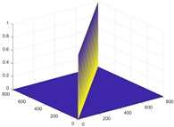
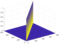
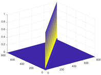
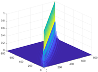
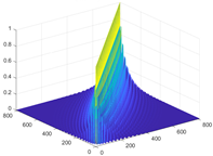
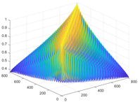
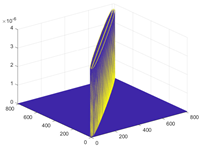
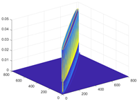
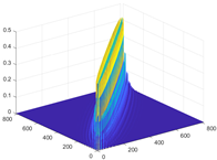
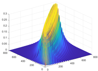
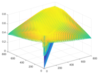
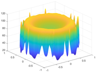
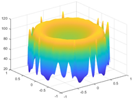
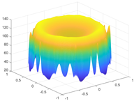
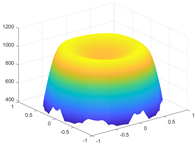
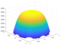
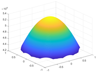
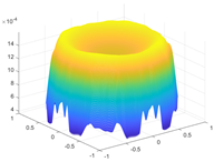
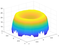
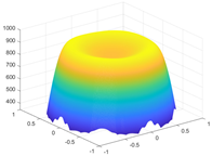
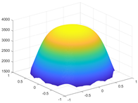
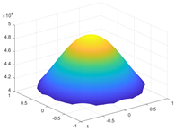
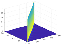
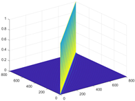
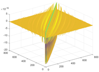
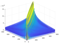
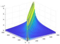
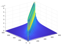
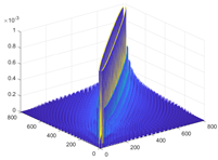
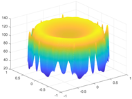
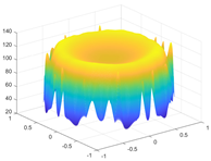
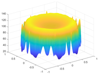
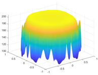
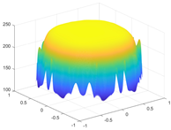
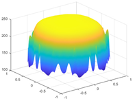
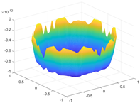
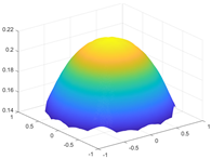
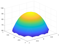
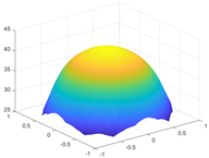
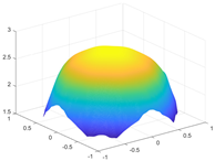
Table 1 shows the three-dimensional distributions of D₂ when using (10) and (19) under various values of Γ and p. The sum of each column of the sensitivity matrix SD₂ in three dimensions is also visualized in Table 1. To clearly show the differences of D₂ or SD₂ as Γ or p changes, we also calculated their differences before and after multiplying D₂ by S, as shown in Table 1.

Table 1. Distributions of D₂ and SD₂ along with Γ or p changes.

D2 with Gaussian Kernel Function $g(R,R^{\prime })=e^{-\Vert R-R^{\prime }\Vert /(2{\Gamma }^2)}$
Γ	0.01	0.05	0.10	0.20	0.30	1.00
D2 distribution
$e^{-\Vert R-R^{\prime }\Vert /{(2{\Gamma }^{\prime })}^2)}-e^{-\Vert R-R^{\prime }\Vert /(2{\Gamma }^2)}$, (Γ’, Γ) = (0.10, 0.05), (0.20,0.10), (0.30, 0.20), (1.00, 0.30).
Distributed column sums of SD2
Difference between two adjacent summed columns of SD2
D2 with Power Function $k(R,R^{\prime })={(1+\Vert d(R,R^{\prime }){\Vert }^p/c)}^{-1}$
p	0.001	0.01	0.10	1.00	5.00	10.00
D2 distribution
${(1+d{(R,R^{\prime })}^{p+1}/c)}^{-1}-{(1+d{(R,R^{\prime })}^{p^{\prime }}/c)}^{-1}$, (p’, p) = (0.01, 0.001), (0.01,0.10), (1.00,0.10), (5.00,1.00), (10.00, 5.00).
Distributed column sums of SD2
Difference between two adjacent summed columns of SD2

As Γ or p is changed, the distribution of D₂ can mostly manifest as a diagonally dominant form, leading to a sufficient approximation for a perfectly diagonal matrix. According to various forms of D₂, we turn the issue to solve (1) to

$$D_{1}S{D}_2\sigma =D_{1}U,\hspace{0.33em}s.t.,\hspace{0.33em}{D}_2=\{g(R,R^{\prime })\}\hspace{0.17em}or\hspace{0.33em}\{k(R,R^{\prime })\}\in R^{n\times n}$$

(20)

where g(R, R′) is computed by (10) and k(R, R′) by (19). In terms of the typical EIT algorithm, (20) can be solved by minimizing the following objective function:

$$\min z=\Vert D_{1}S{D}_2\sigma -D_{1}U\Vert$$

(21)

Any optimization algorithm is principally applicable to solve (21). Generally, when using a diagonally dominant matrix, the following conclusion holds.

Theorem 2.

The solution of (21) has a smaller condition number than that of (1) if using the L₂ norm.

Proof of the theorem is shown in Appendix A (Theorem A2). On the other hand, the two diagonally dominant matrices include the parameters Γ and p, and we demonstrate their effective range through the experiment presented below.

4. Simulation and Evaluation

Simulations and actual experiments were performed to evaluate the effectiveness of our proposed methods along typical EIT reconstruction algorithms. In all simulations and experiments, to reduce the conditional number of S and improve EIT imaging quality, D₁ was constructed as follows:

$$D_1=diag\left\{d_i\right\},\hspace{0.33em}{d}_i=(1/{\displaystyle {\sum }_{j=1}^{812}\left|s_{ij}\right|})/{\max }_j(1/{\displaystyle {\sum }_{j=1}^{812}\left|s_{ij}\right|})$$

(22)

where the effect of D₁ is only the most used normalization form, while D₁ can respond to various EIT algorithms.

The 2-norm condition number of the sensitivity matrix S is given by

$$cond(S)={\mu }_{\max }(S)/{\mu }_{\min }(S)$$

(23)

where μ_max(S) and μ_min(S) denote the maximum and minimum non-zero singular values of the sensitivity matrix S, respectively.

EIT quality is evaluated by two typical indexes [32]. One is the correlation coefficient (CC):

$$CC={(\Delta \sigma -\Delta \overline{\sigma })}^T(\Delta {\sigma }^{*}-\Delta {\overline{\sigma }}^{*})/\sqrt{\Vert \Delta \sigma -\Delta \overline{\sigma }\Vert ·\Vert \Delta {\sigma }^{*}-\Delta {\overline{\sigma }}^{*}\Vert }$$

(24)

where ∆σ and ∆σ* represent the specific gray values of the reconstructed and original images, respectively. Both $\Delta \overline{\sigma }$ and $\Delta {\overline{\sigma }}^{*}$ are their respective means. The other is the relative error (RE):

$$RE=\Vert \Delta \sigma -\Delta {\sigma }^{\ast }\Vert /\Vert \Delta {\sigma }^{\ast }\Vert$$

(25)

The two indexes have typically and frequently been used to evaluate EIT reconstruction quality.

4.1. Simulation on a Set of Typical EIT Models

Simulations were performed using COMSOL 6.3 and MATLAB 2024b software on a PC equipped with an Intel^® Core™ i7 3.4 GHz CPU and 20 GB of RAM. The circular detection field Ω was divided into 812 pixels. The measurements were obtained by a 16-electrode EIT system when the excitation mode employed an adjacent excitation measurement method, and 208 measurements were obtained. The original sensitivity matrix is S ∈ R^208×812. Eleven simulation models with various features termed M1~M11 were used to evaluate EIT quality, where the conductivity of blue background pixels in each model was set at 0.1 S/m, and the conductivity of red target pixels was set at 0.3 S/m.

As the representative example of diagonally dominant matrices, D₂ uses the Gaussian kernel or the power function. All models were reconstructed by the three algorithms LW, TR, and ARW using the same measurements, while the sensitivity matrix S was updated as D₁SD₂. Additionally, since the parameters in the TR algorithm can affect the reconstruction quality, we placed their optimal value in the range [10⁻⁶, 10⁰], and fixed the optimal value in all experiments. And the ARW algorithm had two hyperparameters, which included regularization λ and the norm of the regularization term. The range of regularization λ of ARW is the same as TR and the range of the norm of the regularization term p is [10⁻², 2.0]. The imaging quality of all models was visually compared by target shapes, artifacts, positions, as well as two evaluation indexes, RE and CC. Also, we took their best images with the smallest RE and largest CC over all candidate values as comparisons.

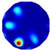
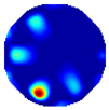
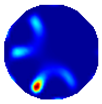
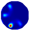
Table 2 shows the reconstruction results along eleven models, M1~M11, and their relative CCs and REs, by LW, TR, and ARW with D₁ and two different forms of D₂. According to Table 2, all reconstructed images from the LW, TR, and ARW algorithms with D₁ and D₂ have better imaging quality than those from the same algorithms with S itself, with more precise image targets and reduced artifacts, essentially for the LW algorithm, which was unable to fully reconstruct the targets for models M2, M3, M4, and M5 using the original sensitivity matrix S. However, by applying left- and right-matrix multiplication, the targets of these models could be successfully reconstructed, and image clarity improved. For the TR algorithm, the original method exhibited significant central artifacts. The method proposed in this paper not only reduces these central artifacts but also enhances the contrast between the targets and the background. For the ARW algorithm, which is known for its superior performance in imaging small targets, there were still considerable artifacts at the edges of the targets. After employing the optimized method, the imaging of the target edges became clearer, and the precision was enhanced further.

Table 2. Reconstructed images by LW, TR and ARW algorithms with the new sensitivity matrix.

	M1	M2	M3	M4	M5	M6	M7	M8	M9	M10	M11
Original image
LW by S
RE	0.4190	0.5236	0.4786	0.5935	0.7350	0.5782	0.7128	0.4522	0.8123	0.5480	0.5089
CC	0.6489	0.5165	0.4929	0.4441	0.3515	0.4649	0.2986	0.4906	0.1891	0.2752	0.6696
LW by S with Gaussian kernel
RE	0.2767	0.3185	0.3571	0.3851	0.4094	0.4424	0.4793	0.3982	0.5202	0.4725	0.4036
CC	0.8479	0.7282	0.6675	0.6305	0.6754	0.5661	0.3923	0.5888	0.2481	0.3977	0.7106
LW by S with power function
RE	0.3047	0.3611	0.3857	0.4360	0.4707	0.4904	0.5490	0.4219	0.5344	0.5058	0.4092
CC	0.7934	0.6616	0.5975	0.5632	0.5678	0.5288	0.3548	0.5371	0.2299	0.3600	0.7171
TR
RE	0.2706	0.2963	0.3014	0.3602	0.3224	0.3568	0.3630	0.3472	0.3402	0.3824	0.3420
CC	0.8736	0.7633	0.7808	0.5991	0.7184	0.6657	0.5308	0.7083	0.3994	0.5004	0.7530
TR by S with Gaussian kernel
RE	0.2588	0.2677	0.2826	0.2831	0.3001	0.3059	0.3225	0.3434	0.4384	0.3582	0.2353
CC	0.8948	0.8143	0.8173	0.7327	0.7656	0.7640	0.6289	0.7407	0.4879	0.6334	0.9004
TR by S with power function
RE	0.2576	0.2713	0.2824	0.2747	0.2842	0.2916	0.3149	0.3504	0.4139	0.3401	0.2017
CC	0.8896	0.8074	0.8196	0.7455	0.8008	0.7831	0.6657	0.7290	0.5148	0.6735	0.9331
ARW
RE	0.3174	0.3049	0.3159	0.2462	0.2717	0.2885	0.2316	0.3482	0.5228	0.3122	0.2211
CC	0.8495	0.7973	0.8124	0.8187	0.8510	0.8095	0.7926	0.6745	0.5917	0.7277	0.9185
ARW by S with Gaussian kernel
RE	0.2989	0.2827	0.3168	0.2204	0.2602	0.2998	0.1769	0.3054	0.2002	0.2904	0.2164
CC	0.8568	0.8492	0.8214	0.8617	0.8768	0.8270	0.8892	0.7673	0.7754	0.7951	0.9226
ARW by S with power function
RE	0.3033	0.2865	0.3154	0.2231	0.2640	0.2995	0.1610	0.3177	0.2125	0.2925	0.2200
CC	0.8568	0.8385	0.8170	0.8388	0.8828	0.8389	0.9072	0.7477	0.7464	0.7743	0.9280

As shown in the CCs and REs, the reconstructed image quality of all models using the proposed method improved, with higher CCs and lower REs. The red number in the table of each image shows its best value. With the increase in the target number and decrease in the target size, the CCs of all models decreased, while the REs increased, indicating lower imaging accuracy. However, after multiplying D₁ and D₂ on the left and right sides of S, no matter which Gaussian kernel or power function was used, the accuracy of all the models significantly increased. These results show that the two types of matrices can effectively improve the quality of the reconstructed image.

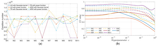
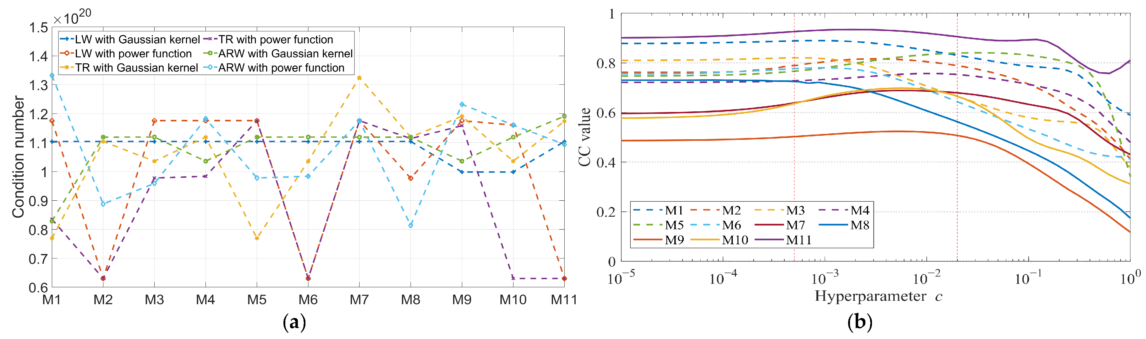
Figure 3a shows the differences in condition numbers between the sensitivity matrix S and D₁SD₂ along with the eleven models. As seen, after multiplying D₁ and D₂ by S, the condition numbers of D₁SD₂ are lower than those of the original sensitivity matrix S. This result indicates that the left- and right-multiplying matrices can optimize solution stability and improve imaging accuracy from another perspective. Among all models, the value of λ was fixed at its optimal value. At the optimal λ value, we multiplied D₂ with the Gaussian or power functions by S. Various values of Γ or p can affect their relative EIT reconstruction quality. Additionally, the value of c can affect the effect of D₂ when using the power function, as shown in Figure 3b. The parameter c governs the resolution or scale of d(R, R′), playing a role analogous to the bandwidth of a kernel function. In addition to the previously adopted value of c = 0.001, we systematically investigated its variation over the interval [10⁻⁵, 1.0] and analyzed the corresponding relationship with the correlation coefficient (CC) of the reconstructed images.

Figure 3. Compared condition numbers in 11 models: (a) D₂ with Guassian kernel; (b) c value in power function.

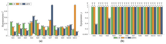
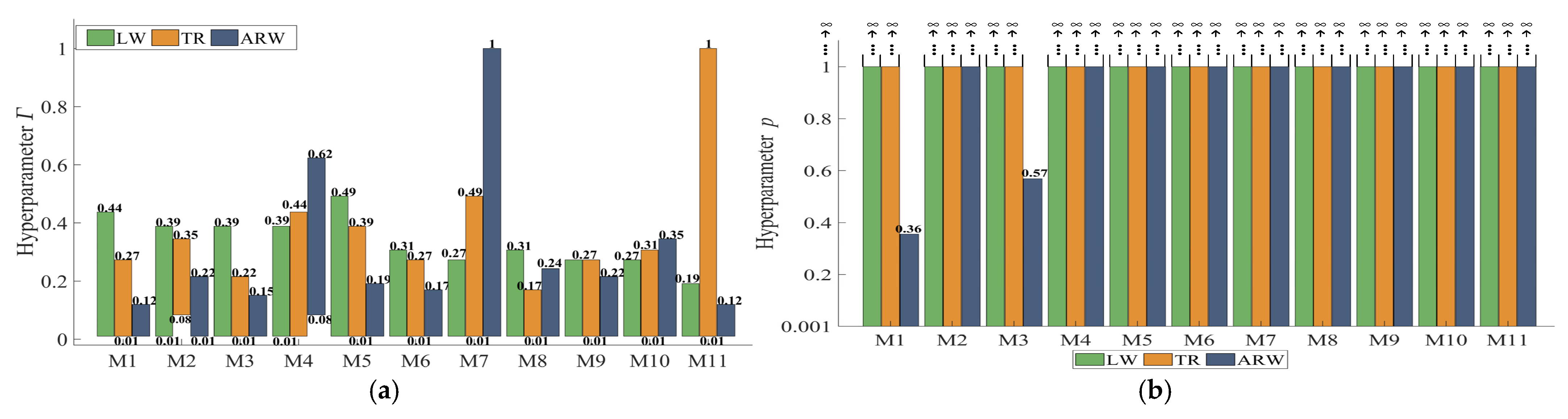
As shown in Figure 3b, within the hyperparameter range of c = [10⁻⁵, 1], we plotted the CC curves for 11 models; the CC values remain consistently high across a relatively broad range of c, specifically from 5 × 10⁻³ to 2 × 10⁻², indicating that the quality of EIT imaging can be stably maintained at a favorable level within this range. This wide permissible interval facilitates the convenient selection of an effective c value in practical implementations. Figure 4 shows the range of Γ or p by which the LW, TR, and ARW algorithms with D₁SD₂ can obtain a higher CC value than those with S. Specifically, the range tends to infinity in most models when using the power function to D₂. These results indicate that improving the condition number of S can enhance EIT reconstruction quality.

Figure 4. Valid range of Γ or p by which the three algorithms have higher CC values than the existing ones. (a) D₂ with Guassian kernel; (b) D₂ with power function.

4.2. Test and Comparison in Noisy Conditions

To evaluate the noise robustness of the proposed method in this study, we added 10% Gaussian white noise to the measurement data generated by COMSOL simulations. This noise level is commonly encountered in existing EIT reconstruction processes and is employed to mimic the inevitable random disturbances present in actual measurements. The corresponding results are presented in Table 3.

Table 3. Experimental comparison of three EIT reconstruction algorithms under noisy conditions (with 10% Gaussian white noise added).

	M1	M2	M3	M4	M5	M6	M7	M8	M9	M10	M11
Original image
LW by S
RE	0.4212	0.5220	0.4773	0.5847	0.7292	0.5969	0.6921	0.4451	0.8591	0.5966	0.4882	0.5829 ± 0.1338
CC	0.6460	0.5078	0.4934	0.4410	0.3504	0.4502	0.2971	0.4832	0.1793	0.2744	0.6639	0.4352 ± 0.1502
LW by S with Gaussian kernel
RE	0.2788	0.3232	0.3661	0.3810	0.4075	0.4441	0.4819	0.4058	0.5127	0.4851	0.3900	0.4069 ± 0.0710
CC	0.8452	0.7275	0.6535	0.6335	0.6679	0.5691	0.3968	0.5822	0.2455	0.3922	0.7018	0.5832 ± 0.1743
LW by S with power function
RE	0.3089	0.3673	0.3882	0.4271	0.4683	0.4808	0.5458	0.4205	0.5423	0.5372	0.3953	0.4438 ± 0.0782
CC	0.7889	0.6585	0.5911	0.5620	0.5621	0.5299	0.3586	0.5322	0.2248	0.3589	0.7118	0.5344 ± 0.1655
TR
RE	0.3140	0.3138	0.3634	0.4298	0.3356	0.4227	0.4379	0.3649	0.4585	0.4766	0.4775	0.3995 ± 0.0630
CC	0.8260	0.7326	0.6442	0.5336	0.6865	0.5804	0.4241	0.6598	0.2168	0.2249	0.4571	0.5442 ± 0.1978
TR by S with Gaussian kernel
RE	0.2873	0.2908	0.3372	0.4261	0.3101	0.3799	0.4022	0.3492	0.5202	0.4215	0.4589	0.3803 ± 0.0738
CC	0.8546	0.7844	0.7162	0.6091	0.7436	0.6362	0.5674	0.7375	0.3089	0.4037	0.6144	0.6342 ± 0.1628
TR by S with power function
RE	0.2865	0.2855	0.3381	0.4040	0.2992	0.3819	0.3741	0.3559	0.5012	0.4102	0.4678	0.3731 ± 0.0707
CC	0.8508	0.7882	0.7108	0.6214	0.7620	0.6326	0.5979	0.7262	0.3103	0.4148	0.6054	0.6382 ± 0.1601
ARW
RE	0.4033	0.3198	0.3920	0.2818	0.2826	0.3371	0.2864	0.3658	0.3405	0.4141	0.3721	0.3450 ± 0.0486
CC	0.6881	0.7311	0.5920	0.7152	0.7976	0.6874	0.6353	0.6372	0.2421	0.3417	0.7472	0.6195 ± 0.1732
ARW by S with Gaussian kernel
RE	0.3114	0.2794	0.3357	0.2371	0.2680	0.3041	0.2371	0.3352	0.2996	0.3623	0.2753	0.2950 ± 0.0403
CC	0.8460	0.8422	0.7628	0.8242	0.8543	0.7828	0.7725	0.7134	0.4885	0.5775	0.8712	0.7578 ± 0.1222
ARW by S with power function
RE	0.3159	0.2848	0.3359	0.2769	0.2722	0.3234	0.2803	0.3572	0.3343	0.4001	0.2698	0.3137 ± 0.0416
CC	0.8471	0.7978	0.7311	0.7392	0.8153	0.7239	0.6974	0.6560	0.4721	0.5275	0.8532	0.7146 ± 0.1234

As shown in Table 3, the reconstruction quality of all algorithms degrades to varying degrees under noisy perturbations, with discrete small targets (e.g., models 9 and 10) being particularly affected. Across all test models, the average CC values of the three algorithms decrease by a range of approximately 0.50% to 16.62%, while the average RE values increase by a range of 0.46% to 6.47%. Nevertheless, when the original sensitivity matrix S is replaced by D₁SD₂, the reconstructed images exhibit higher CC values and lower relative errors compared to those obtained with the original matrix. Specifically, the CC value is improved by up to 31.75%, and the relative error is reduced by as much as 34.64% relative to the original results. The last column reports the average fluctuation ranges of CC and RE in various models. These findings demonstrate that the proposed method possesses favorable noise robustness and is capable of achieving high-quality image reconstruction, even under disturbances induced by measurement noise.

4.3. Test on a Set of Actual Models

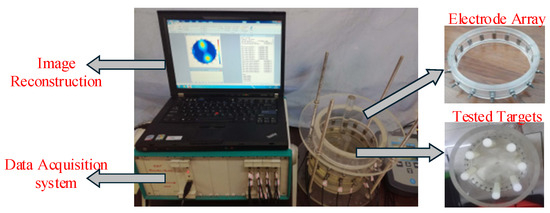
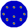
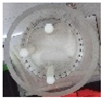
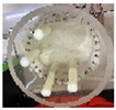
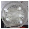
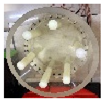
Figure 5 shows that the ERT system consists of data acquisition, a computer, and a sensor of 16 electrodes that are equipped on a cylinder filled in a conductive liquid measuring 16 μS/cm, where the diameter of the cylinder is 160 mm, the size of each electrode is 10 × 20 mm, and a single-excitation single-measurement mode is adopted to obtain 240 measurement values per imaging frame at a system sampling rate of 25 frames per second. A group of rubber rods (objects) are vertically inserted in the cylinder along various positions, where these rod measure 1 cm. The detected field Ω was partitioned into 812 pixels to reconstruct these rod objects.

Figure 5. The ERT system with 16 electrodes.

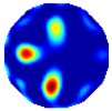
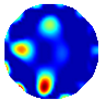
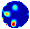
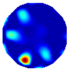
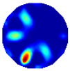
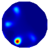
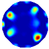
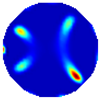
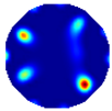
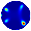
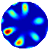
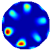
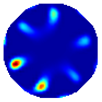
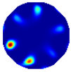
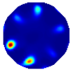
The second column in Table 4 presents the tested models, numbered M12, M13, M14, M15, and M16, while the remaining columns display the reconstructed images obtained by different EIT reconstruction algorithms with D₁SD₂. In addition, we calculated CC and RE for each algorithm. The values enclosed in parentheses represent the CC and RE increments achieved by the algorithms with D₁SD₂ compared with the original imaging algorithm, serving as quantitative metrics to characterize the performance improvement of the EIT reconstruction algorithms with D₁SD₂. The RE and CC values highlighted in red correspond to the optimal performance among all algorithms for each given model. As observed from the experimental results, the EIT methods with D₁SD₂ consistently yield higher correlation coefficients and lower relative errors compared to the original algorithm. For example, for model 14, the original algorithm failed to fully resolve the three closely spaced rods on the right side, whereas the modified approach successful identified the targets in most cases. The last column reports the average fluctuation ranges of CC and RE along various EIT algorithms. These results demonstrate that the EIT algorithms with D₁SD₂ enable more accurate reconstructions of both the positions and the number of targets.

Table 4. Comparison of reconstruction results obtained by different algorithms in actual experiments.

	Original Image	LW by S	LW by S with Gaussian Kernel	LW by S with Power Function	TR	TR by S with Gaussian Kernel	TR by S with Power Function	ARW	ARW by S with Gaussian Kernel	ARW by S with Power Function
M12
	RE	0.3861	0.3678 (−0.0183)	0.3853 (−0.0008)	0.3700	0.3381 (−0.0319)	0.3403 (−0.0297)	0.3865	0.3408 (−0.0457)	0.3847 (−0.0018)	0.3595 ± 0.0258
	CC	0.3765	0.3848 (0.0083)	0.3765 (0.0000)	0.3245	0.4164 (0.0919)	0.4088 (0.0843)	0.3821	0.4028 (0.0207)	0.3864 (0.0043)	0.3960 ± 0.0204
M13
	RE	0.3646	0.3343 (−0.0303)	0.3364 (−0.0282)	0.3662	0.3259 (−0.0403)	0.3248 (−0.0414)	0.3214	0.3094 (−0.0120)	0.3076 (−0.0138)	0.3231 ± 0.0155
	CC	0.3181	0.4089 (0.0908)	0.4047 (0.0866)	0.3191	0.4198 (0.1007)	0.4229 (0.1038)	0.3876	0.4377 (0.0501)	0.4471 (0.0595)	0.4235 ± 0.0236
M14
	RE	0.4032	0.3474 (−0.0558)	0.3552 (−0.0480)	0.3855	0.3238 (−0.0617)	0.3265 (−0.0590)	0.3260	0.3116 (−0.0144)	0.3130 (−0.0130)	0.3296 ± 0.0256
	CC	0.3667	0.5252 (0.1585)	0.4959 (0.1292)	0.3849	0.5422 (0.1573)	0.5356 (0.1507)	0.4606	0.5223 (0.0617)	0.5085 (0.0479)	0.5216 ± 0.0257
M15
	RE	0.3985	0.3943 (−0.0040)	0.3973 (−0.0012)	0.4023	0.3837 (−0.0186)	0.3812 (−0.0211)	0.3573	0.3533 (−0.004)	0.3508 (−0.0065)	0.3768 ± 0.0260
	CC	0.3782	0.4005 (0.0223)	0.3978 (0.0196)	0.3477	0.4086 (0.0609)	0.4100 (0.0623)	0.4275	0.4488 (0.0213)	0.4576 (0.0301)	0.4206 ± 0.0371
M16
	RE	0.4210	0.3741 (−0.0469)	0.3756 (−0.0454)	0.4006	0.3653 (−0.0353)	0.3663 (−0.0343)	0.4056	0.3630 (−0.0426)	0.3676 (−0.0380)	0.3687 ± 0.0070
	CC	0.2487	0.4028 (0.1541)	0.3918 (0.1431)	0.2657	0.4382 (0.1725)	0.4343 (0.1686)	0.2753	0.4523 (0.1770)	0.4216 (0.1463)	0.4235 ± 0.0317

Table 5 compares several representative EIT algorithms. The baseline method is LBP, which only uses the original sensitivity matrix S, while the TR algorithm employs left multiplication of S by the matrix D₁ = (SᵀS + λI)⁻¹ with no right-multiplication operation. In fact, as indicated by (9), the vast majority of existing EIT reconstruction algorithms can be uniformly formulated as applying some form of left-multiplication transformation to S. In contrast, the second strategy involves the right multiplication of S by a Gaussian kernel-based matrix D₂, without applying left multiplication. To ensure a fair comparison, all methods adopt identical configurations, noise levels, parameter tuning strategies, and evaluation metrics. Table 5 summarizes the performance differences between the proposed D₁SD₂ method and the two comparison methods on reconstruction quality, where D₂ is implemented using the Gaussian kernel function as an example. From the comparative results of these original model images listed in Table 4, it is evident that LBP yields the lowest reconstruction quality, while the D₁SD₂ method achieves the highest reconstruction quality. Furthermore, by examining the trends in RE and CC values, it can be observed that the image quality progressively improves from left multiplication, by D₁ alone, to right multiplication, by D₂ alone, and finally to the simultaneous application of D₁SD₂, thereby fully demonstrating the effectiveness of the proposed algorithm.

Table 5. Experimental comparison between D₁SD₂ and existing matrix transformation methods.

	M12	M13	M14	M15	M16
LBP
RE	0.5804	0.5192	0.4943	0.5101	0.4449
CC	0.2657	0.2695	0.3227	0.2658	0.0818
TR (left multiplication of S by D1 without right multiplication by D2)
RE	0.3700	0.3662	0.3855	0.4023	0.4006
CC	0.3245	0.3191	0.3849	0.3477	0.2657
SD2 (right multiplication of S by D2 without left multiplication by D1)
RE	0.3683	0.3250	0.3840	0.4040	0.3978
CC	0.3310	0.3673	0.4017	0.3600	0.2704
TR with D1SD2
RE	0.3381	0.3259	0.3238	0.3837	0.3653
CC	0.4164	0.4198	0.5422	0.4086	0.4382

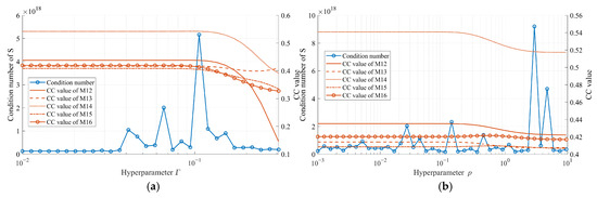
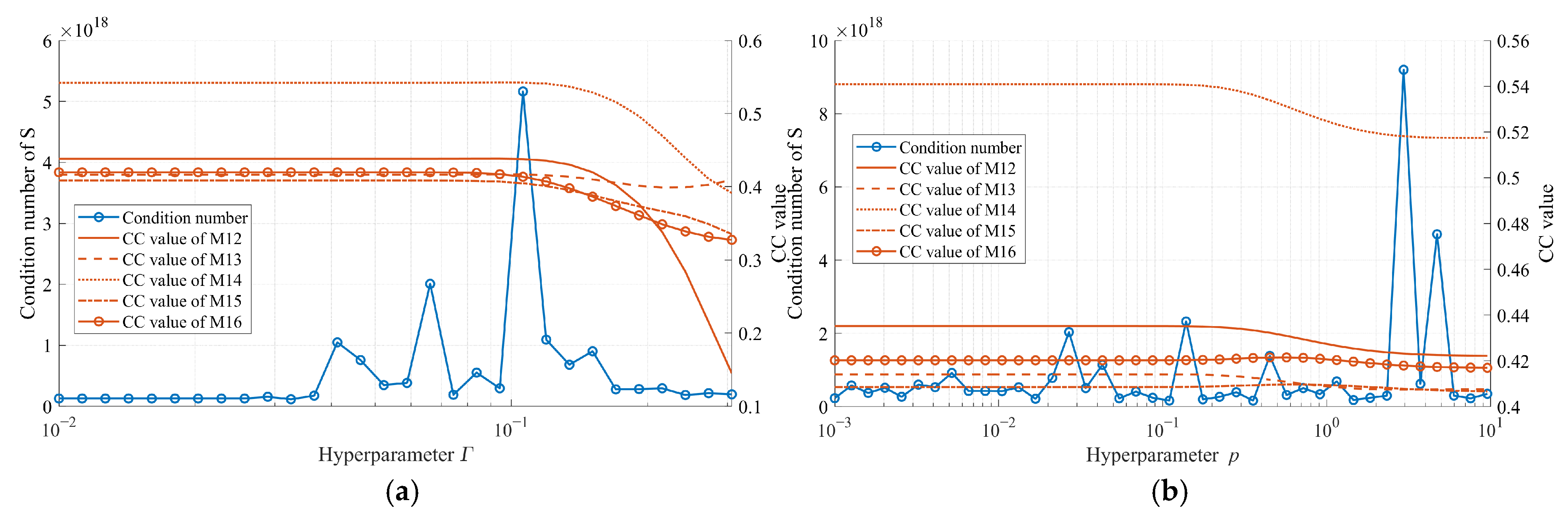
Finally, we present an experimental method for selecting the hyperparameters Γ and p. Given that the theoretical analysis in this paper demonstrated that a smaller condition number is more conducive to improving EIT reconstruction quality, we first determined a reasonable search interval based on the condition number and the specific characteristics of the problem, then discretized this interval, and selected appropriate parameter values through an exhaustive search. Figure 6a,b illustrate how the condition number varies with hyperparameters Γ and p over their respective value ranges, where D₂ is constructed using the Gaussian kernel and the power function, respectively. To reveal the influence of the condition number on the reconstruction effects of five practical models, the corresponding CC value curves are also plotted in the figures. It can be observed that, within fairly wide parameter intervals of Γ and p, the condition number remains at a relatively low level, and the corresponding CC values are also relatively high; however, when the condition number exhibits abnormal fluctuations or a noticeable increase, the CC value decreases accordingly, with this effect being more significant, especially in the case of the Gaussian kernel. This indicates that there is an inevitable correlation between the condition number and reconstruction quality; therefore, we suggest that in practical applications, the interval where the condition number is relatively small should be selected as the reference range for effective parameters.

Figure 6. Variation of sensitivity matrix condition number and CC of five models under different hyperparameters (a) D₂ with Guassian kernel; (b) D₂ with power function.

It should be pointed out that, due to the inherent underdetermined nature and soft-field characteristics of the EIT problem, factors such as the amount of measurement data and the noise level also have an impact on the reconstruction results. Consequently, although improving the condition number is an important factor for enhancing reconstruction quality, it is not yet a sufficient condition. On the other hand, in EIT reconstruction algorithms, the sensitivity matrix is predetermined and remains unchanged during the reconstruction process; this means that both S and D₁SD₂ are determined a priori. Therefore, the real-time performance of each algorithm is determined by the algorithm itself. However, relative to specific application scenarios, when it is necessary to adjust the parameters according to the measurements and the specific application object and to search for better Γ and p values based on the condition number, this increases the computation time and reduces the real-time performance of EIT reconstruction, with the increased time being directly proportional to the number of candidate values for these parameters within the discretized interval. Therefore, we recommend performing an offline parameter search under typical operating conditions to pre-determine a set of optimal parameters. In this way, the precomputed parameters can be directly adopted during the online reconstruction phase, which avoids extra computational overhead and improves real-time performance.

5. Conclusions

Most of the existing EIT reconstruction algorithms are equivalent to multiplying the existing sensitivity matrix on the left and right by two diagonal matrices; thus, these algorithms can be uniformly characterized by the matrix transformation. Note that the stability and quality of EIT reconstruction can be represented by the condition number of the sensitivity matrix. We demonstrate that the left and right multiplications of the sensitivity matrix by its respective diagonal matrix can reduce the condition number. Then, the EIT reconstruction quality can be effectively improved after multiplying the two diagonal matrices. As examples, a Gaussian kernel-based symmetric matrix and a power function-based matrix are used to validate the proposed method. The experimental results further prove the potential of the new sensitivity matrix proposed in this study, which can provide a new theoretical and practical strategy for EIT reconstruction.

In the future, three issues must be focused on. One is how to obtain a better diagonally dominant matrix to reduce the condition number. The second is how to use the best matrix transformation to improve EIT reconstruction accuracy and reliability. Many such matrix transformations are available, and we believe that their various forms have the potential to further improve EIT reconstruction quality. Finally, three-dimensional EIT reconstruction is an important research direction, and therefore, the advancement of the method proposed in this study is anticipated in the future. However, it involves a higher-dimensional sensitivity matrix, enormous computational and storage overhead, as well as more complex soft-field effects; thus, it is necessary to discuss the feasibility, potential advantages, and the computational complexity issues that need to be addressed further when extending the matrix transformation method proposed in this paper to 3D EIT.

References

- Liu, D.; Wang, J.; Shan, Q.; Smyl, D.; Deng, J.; Du, J. DeepEIT: Deep image prior enabled electrical impedance tomography. IEEE Trans. Pattern Anal. Mach. Intell. 2023, 45, 9627–9638. [Google Scholar] [CrossRef] [Scilit] [PubMed]
- Sun, J.; Yang, W. A dual-modality electrical tomography sensor for measurement of gas–oil–water stratified flows. Measurement 2015, 66, 150–160. [Google Scholar] [CrossRef] [Scilit]
- Sun, B.; Yue, S.; Hao, Z.; Cui, Z.; Wang, H. An improved Tikhonov regularization method for lung cancer monitoring using electrical impedance tomography. IEEE Sens. J. 2019, 19, 3049–3057. [Google Scholar] [CrossRef] [Scilit]
- Smyl, D. Electrical tomography for characterizing transport properties in cement-based materials: A review. Constr. Build. Mater. 2020, 244, 118299. [Google Scholar] [CrossRef] [Scilit]
- Ke, X.-Y.; Hou, W.; Huang, Q.; Hou, X.; Bao, X.Y.; Kong, W.X.; Li, C.X.; Qiu, Y.Q.; Hu, S.Y.; Dong, L.H. Advances in electrical impedance tomography-based brain imaging. Mil. Med. Res. 2022, 9, 10. [Google Scholar] [CrossRef] [Scilit] [PubMed]
- Wang, Z.; Liu, X. A regularization structure based on novel iterative penalty term for electrical impedance tomography. Measurement 2023, 209, 112472. [Google Scholar] [CrossRef] [Scilit]
- da Mata, A.M.M.; de Moura, B.F.; Martins, M.F.; Palma, F.H.S.; Ramos, R. Electrical Conductivity Effect on the Performance Evaluation of EIT Systems: A Review. Measurement 2021, 178, 109401. [Google Scholar] [CrossRef] [Scilit]
- Wang, Z.; Yue, S.; Song, K.; Liu, X.; Wang, H. An unsupervised method for evaluating electrical impedance tomography images. IEEE Trans. Instrum. Meas. 2018, 67, 2796–2803. [Google Scholar] [CrossRef] [Scilit]
- Sun, B.; Yue, S.; Cui, Z.; Wang, H. A new linear back projection algorithm to electrical tomography based on measuring data decomposition. Meas. Sci. Technol. 2015, 26, 1270–1283. [Google Scholar] [CrossRef] [Scilit]
- Soleimani, M.; Powell, C.E.; Polydorides, N. Improving the forward solver for the complete electrode model in EIT using algebraic multigrid. IEEE Trans. Med. Imag. 2005, 24, 577–583. [Google Scholar] [CrossRef] [Scilit] [PubMed]
- Isaacson, D.; Mueller, J.L.; Newell, J.C.; Siltanen, S. Reconstructions of chest phantoms by the D-bar method for electrical impedance tomography. IEEE Trans. Med. Imaging 2004, 23, 821–828. [Google Scholar] [CrossRef] [Scilit] [PubMed]
- Wang, M. Inverse solutions for electrical impedance tomography based on conjugate gradients methods. Meas. Sci. Technol. 2002, 13, 101–117. [Google Scholar] [CrossRef] [Scilit]
- Murphy, E.K.; Mahara, A.; Halter, R.J. A novel regularization technique for microendoscopic electrical impedance tomography. IEEE Trans. Med. Imag. 2016, 35, 1593–1603. [Google Scholar] [CrossRef] [Scilit] [PubMed]
- Yang, W.Q.; Spink, D.M.; York, T.A.; McCann, H. An image-reconstruction algorithm based on Landweber’s iteration method for electrical-capacitance tomography. Meas. Sci. Technol. 1999, 10, 1065. [Google Scholar] [CrossRef] [Scilit]
- Liu, X.; Yue, S.; Ren, H. A λ-level partition-based linear back projection algorithm to electrical resistance tomography. In Proceedings of the 2022 IEEE International Instrumentation and Measurement Technology Conference (I2MTC), Ottawa, ON, Canada, 16–19 May 2022; IEEE: Piscataway, NJ, USA, 2022; pp. 1–6. [Google Scholar] [CrossRef] [Scilit]
- Ding, M.; Yue, S.; Li, J.; Wang, Y.; Wang, H. Second-order sensitivity coefficient based electrical tomography imaging. Chem. Eng. Sci. 2019, 199, 40–49. [Google Scholar] [CrossRef] [Scilit]
- Liu, S.; Cao, R.; Huang, Y.; Ouypornkochagorn, T.; Ji, J. Time Sequence Learning for Electrical Impedance Tomography Using Bayesian Spatiotemporal Priors. IEEE Trans. Instrum. Meas. 2020, 69, 6045–6057. [Google Scholar] [CrossRef] [Scilit]
- Ding, M.; Yue, S.; Li, J.; Li, Q.; Wang, H. Optimal similarity norm for electrical tomography based on bregman divergence. Rev. Sci. Instrum. 2020, 91, 033707. [Google Scholar] [CrossRef] [Scilit] [PubMed]
- Yue, S.; Yue, S.; Zeng, M. Measurement and application of soft-field effect in electrical tomography. IEEE Trans. Instrum. Meas. 2025, 74, 1–12. [Google Scholar] [CrossRef] [Scilit]
- de Moura, H.L.; Pipa, D.R.; do Nascimento Wrasse, A.; da Silva, M.J. Image reconstruction for electrical capacitance tomography through redundant sensitivity matrix. IEEE Sens. J. 2017, 17, 8157–8165. [Google Scholar] [CrossRef] [Scilit]
- Dong, F.; Yue, S.; Liu, X.; Wang, H. Determination of hyperparameter and similarity norm for electrical tomography algorithm using clustering validity index. Measurement 2023, 216, 112976. [Google Scholar] [CrossRef] [Scilit]
- Barber, D.C.; Brown, B.H.; Avis, N.J. Image reconstruction in electrical impedance tomography using filtered back-projection. In Proceedings of the 1992 14th Annual International Conference of the IEEE Engineering in Medicine and Biology Society, Paris, France, 29 October–1 November 1992; IEEE: Piscataway, NJ, USA, 1992; pp. 1691–1692. [Google Scholar] [CrossRef] [Scilit]
- Xu, Y.; Han, B.; Dong, F. A new regularization algorithm based on the neighborhood method for electrical impedance tomography. Meas. Sci. Technol. 2018, 29, 085401. [Google Scholar] [CrossRef] [Scilit]
- Zhang, Q.; Mo, H.; Li, R.; Liang, C.; Luo, J.; Bespal’Ko, A.A. Image reconstruction method based on wavelet fusion in electrical capacitance tomography with rotatable electrode sensor. Measurement 2024, 238, 115354. [Google Scholar] [CrossRef] [Scilit]
- Liu, X.; Wang, Y.; Li, D.; Li, L. Sparse reconstruction of EMT based on compressed sensing and L regularization with the split Bregman method. Flow Meas. Instrum. 2023, 94, 102473. [Google Scholar] [CrossRef] [Scilit]
- Dang, C.; Bellis, C.; Darnajou, M.; Ricciardi, G.; Mylvaganam, S.; Bourennane, S. Practical comparisons of EIT excitation protocols with applications in high-contrast imaging. Meas. Sci. Technol. 2021, 32, 085110. [Google Scholar] [CrossRef] [Scilit]
- Bagshaw, A.P.; Liston, A.D.; Bayford, R.H.; Tizzard, A.; Gibson, A.P.; Tidswell, A.T.; Sparkes, M.K.; Dehghani, H.; Binnie, C.D.; Holder, D.S. Electrical impedance tomography of human brain function using reconstruction algorithms based on the finite element method. NeuroImage 2003, 20, 752–764. [Google Scholar] [CrossRef] [Scilit] [PubMed]
- Hanke, M.; Neubauer, A.; Scherzer, O. A convergence analysis of the Landweber iteration for nonlinear III-posed problems. Numer. Math. 1995, 72, 21–37. [Google Scholar] [CrossRef] [Scilit]
- Hansen, P.C.; O’Leary, D.P. The use of the L-curve in the regularization of discrete ill-posed problems. SIAM J. Sci. Comput. 1993, 14, 1487–1503. [Google Scholar] [CrossRef] [Scilit]
- Li, J.; Yue, S.; Ding, M.; Cui, Z.; Wang, H. Adaptive Lp regularization for electrical impedance tomography. IEEE Sens. J. 2019, 19, 12297–12305. [Google Scholar] [CrossRef] [Scilit]
- Liu, Z.; Yang, Y. Multimodal Image Reconstruction of Electrical Impedance Tomography Using Kernel Method. IEEE Trans. Instrum. Meas. 2022, 71, 1–12. [Google Scholar] [CrossRef] [Scilit]
- Wang, Z.; Sun, Y.; Li, J. Posterior Approximate Clustering-Based Sensitivity Matrix Decomposition for Electrical Impedance Tomography. Sensors 2024, 24, 333. [Google Scholar] [CrossRef] [Scilit] [PubMed]
- Schulman, L.J.; Sinclair, A. Analysis of a classical matrix preconditioning algorithm. In Proceedings of the Forty-Seventh Annual ACM Symposium on Theory of Computing, Portland, OR, USA, 14–17 June 2015; Association for Computing Machinery: New York, NY, USA, 2015; pp. 831–840. [Google Scholar] [CrossRef] [Scilit]
Disclaimer/Publisher’s Note: The statements, opinions and data contained in all publications are solely those of the individual author(s) and contributor(s) and not of MDPI and/or the editor(s). MDPI and/or the editor(s) disclaim responsibility for any injury to people or property resulting from any ideas, methods, instructions or products referred to in the content. |
© 2026 by the authors. Licensee MDPI, Basel, Switzerland. This article is an open access article distributed under the terms and conditions of the Creative Commons Attribution (CC BY) license.