Theoretical Solutions for Tunnels Excavated in Strain-Softening Rock Masses Considering Support

Abstract

The collaborative load-bearing behavior between the rock mass and support is critical for tunnel support design. This study proposes a strain-softening analysis method for circular tunnels during construction and presents an efficient solution strategy, termed the “Support Load Approximation Strategy” (SLAS), to solve the collaborative load-bearing problem. The rock mass is assumed to be isotropic, following the Mohr–Coulomb criterion, under hydrostatic stress conditions. During the stepwise calculation, a new ring is automatically added at each step, and the positions of all previous rings are updated, with elastic or plastic formulations automatically selected based on the state of each ring. The GRC and plastic radii (R_p and R_s) curves obtained by the proposed method show excellent agreement with existing benchmark results, with relative errors of 3.73% for the GRC, 1.47% for R_s, and 3.40% for R_p, confirming the correctness and accuracy of the proposed algorithm. Furthermore, when compared to the Incremental Support Load Method (ISLM) and the binary search method, SLAS improves computational efficiency by 14.2 times and 67%, and accuracy by 70% and 53%, respectively. When higher precision is required, SLAS maintains an efficiency gain of 82.8 times over ISLM with comparable accuracy. Compared to traditional elastic-plastic analysis methods, the proposed approach simplifies the computational process, reduces complexity, offers both high accuracy and fast computation speed, and serves as a practical tool for tunnel engineering support design.

1. Introduction

As society continues to develop, an increasing number of tunnels are being constructed [1,2,3,4]. Understanding the collaborative load-bearing behavior and load distribution relationship between the rock mass and support is a prerequisite for the design of supports during the tunnel construction phase [5,6,7]. In the 1930s, the convergence confinement method (CCM), developed based on elastoplastic theory, provided a useful tool for studying the interaction between rock masses and supports. CCM comprises three parts [8]: the longitudinal deformation profile (LDP), ground reaction curve (GRC), and support characteristic curve (SCC). By determining the intersection points of the GRC and SCC, the loads borne by the rock mass and support, as well as their respective load-sharing ratios, can be determined.

Researchers often treat rock masses as either elastic models or ideal elastoplastic models [7,9,10,11,12]. They have proposed various methods with explicit expressions for solving the GRC, which simplifies the solution of the CCM. However, in the field of underground engineering, rock masses often exhibit softening behavior [1,13,14,15,16,17]. Therefore, studying the mechanical behavior of rock masses with strain-softening characteristics is of significant engineering importance. For strain-softening rock masses, attempts at elastoplastic analysis are limited. This may be due to the constantly changing mechanical properties of rock masses, which make the solution process more complex. Some experts have proposed some methods for solving the GRC that consider strain softening in rock masses. For instance, the method proposed by Alonso et al. (2003) [18] appears theoretically sound. However, its application in practical engineering situations can become quite complex. Guan et al. (2007) [19] obtained solutions for circular tunnels based on strain-softening theory, but only considered changes in cohesion and dilation angle, neglecting changes in the internal friction angle. In Lee’s method [1], the number of rings within the plastic zone remains fixed and does not increase as the plastic zone expands. This creates a conflict: using too few rings compromises accuracy, whereas using too many wastes computational resources. Xu et al. (2021) [15] made improvements to Lee’s method [1]; however, after the plastic zone is formed, an additional assumption is required in each calculation step. This increases the complexity and makes the algorithm difficult to follow. Consequently, a key unresolved problem is the need for an elastoplastic analysis method for strain-softening rocks that is both accurate and efficient, yet simple to implement and understand.

The SCC is another crucial component of the CCM. Different supports have different methods for solving the SCC [20,21]. In previous studies, the solutions for GRC and SCC have mostly focused on elastoplastic rock masses [20,22]. For rock masses considering softening characteristics, the process of solving GRC and SCC will be more complex. Currently, research in this area is relatively weak. Based on this, Ren et al. (2023) [21] proposed the “Incremental Support Load Method (ISLM).” Assuming in a certain calculation step, the actual loads borne by the rock mass and lining are as shown in Figure 1a, where the load borne by the support is represented by the yellow portion, and the load borne by the rock mass is represented by the blue portion.

Figure 1. Solution schematic diagram of the Incremental Support Load Method (ISLM). Yellow represents the support load, and blue represents the surrounding rock load. (a) Load distribution on rock mass and lining; (b) Large load increments approach; (c) Small load increments approach.

The solution approach of ISLM is as follows [21]: in each calculation step, incrementally increase the support’s load in equal increments, gradually approaching the true value. With each increment of load, calculations and comparative analyses are required until the difference between the computed results of the support and the actual results is less than a certain constant. However, achieving optimal computational efficiency and accuracy simultaneously with ISLM is challenging. If the increment of load added each time is large, the computation speed will be faster, but the accuracy may decrease, as shown in Figure 1b. Conversely, if the increment of load added each time is small, the accuracy may increase, but the computation speed will be slower, as shown in Figure 1c. ISLM requires a balance between computational efficiency and accuracy. Therefore, further exploration is needed for the solution methods of GRC and SCC, considering the softening characteristics of rock masses.

To address the first problem—namely, the conflict between efficiency and accuracy in existing strain-softening rock analysis methods—this paper proposes a novel elastoplastic analysis method. In contrast to Lee’s fixed-ring approach [1], our method automatically adds a new calculation ring during each stress release step, allowing the number of rings to grow dynamically with the plastic zone. This ensures both efficient use of computational resources and high accuracy. Furthermore, to overcome the complexity of Xu et al.’s method and the numerical instability of calculating from the outermost ring [15,23], our method innovatively uses the “second-to-last ring” instead of the “outermost ring” as the starting point for calculations. This simple but powerful strategy simplifies the computational procedure, renders the algorithm easier to understand, and maintains high accuracy.

To address the second problem (the efficiency-accuracy trade-off of the ISLM) [21], this paper introduces the “Support Load Approximation Strategy (SLAS)”. Unlike the ISLM, which relies on uniform load increments, the SLAS exploits the fundamental characteristic that the rock mass bears the majority of the load while the support bears a small portion. It operates in two stages: a “Global Approximation” stage to quickly estimate the support load, followed by a “Local Approximation” stage using a binary search to refine the result. This hybrid approach is designed to simultaneously achieve high computational efficiency and accuracy.

2. Statement of the Problem

2.1. Geometrical Relationship

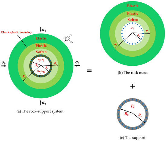
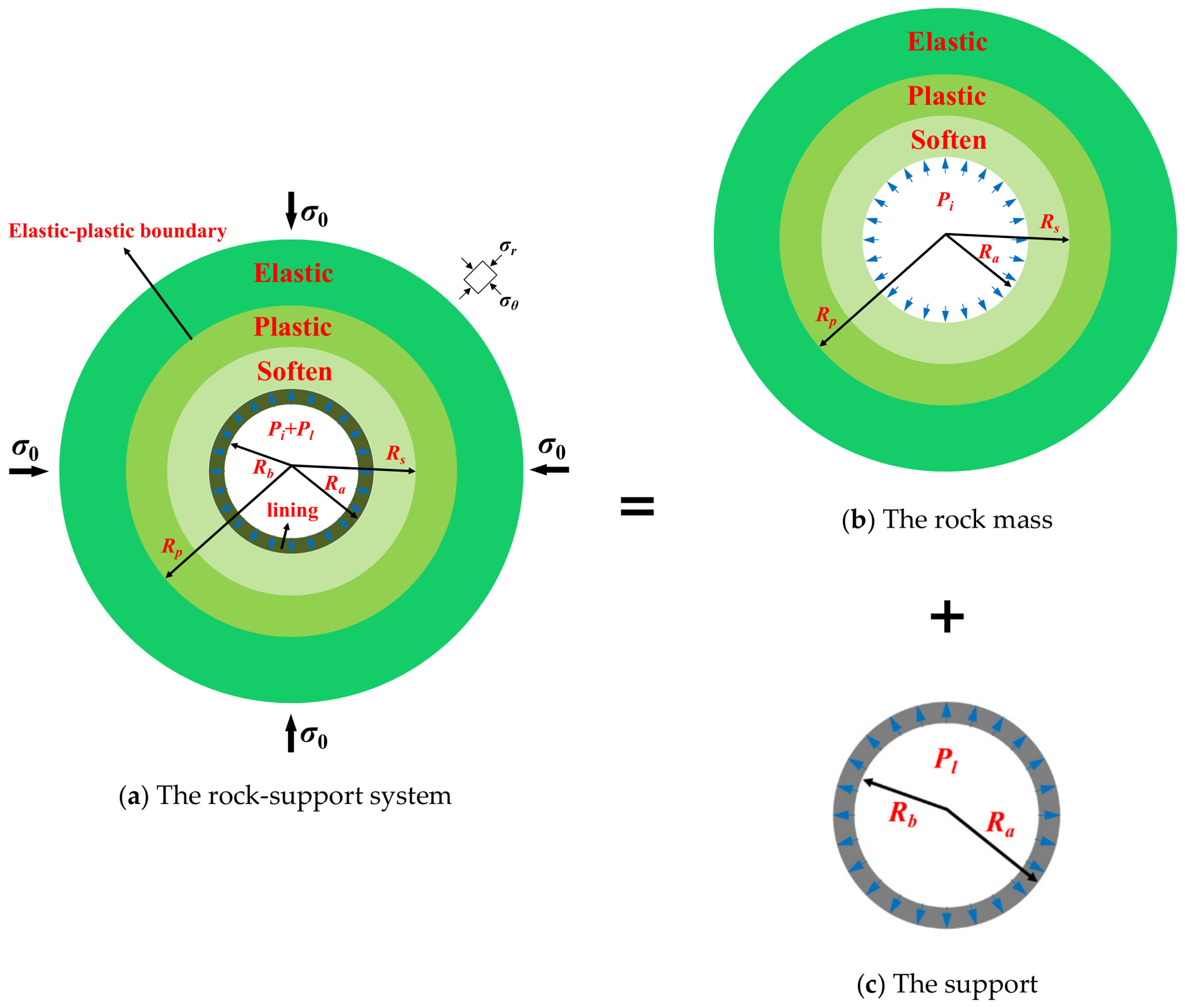
Figure 2a presents the schematic diagram illustrating the collaborative load-bearing process of the rock-support system. A circular tunnel with a radius of R_a is situated in a homogeneous rock mass with isotropic properties and a hydrostatic stress field of σ₀. The rock mass follows the Mohr–Coulomb criterion [24]. The support is considered as a linear elastic model with an internal radius of R_b. There is no tangential sliding between the rock mass and the lining [21]; therefore, only a radial contact force P_l exists between them.

Figure 2. The collaborative load-bearing of the rock-support system.

The rock-support system is divided into the rock mass (Figure 2b) and the support (Figure 2c). For the rock mass, the inner surface of the tunnel receives both the virtual support force P_i provided by the heading face and the reaction force P_l from the support [21]. The force exerted by the rock mass on the support is also P_l.

When the internal support force of the rock mass is less than the critical support force P_ic, a plastic zone with a radius of R_p is formed around the tunnel. In this area, the mechanical properties of the material are reduced. In some cases, in addition to the plastic zone R_p, there may be another residual zone with a radius of R_s. In this area, the mechanical properties of the material are further reduced. In this study, it is defined that compressive stress is positive and contraction displacement is positive.

In the Figure 2, σ₀ represents the original rock stress, σ_θ and σ_r represent the tangential stress and radial stress, respectively.

2.2. Governing Equations

In polar coordinates, the equilibrium differential equation, geometric equation, and physical equation for the plane strain axisymmetric problem are as follows:

$${\displaystyle \frac{d{\sigma }_r}{dr}}+{\displaystyle \frac{{\sigma }_r-{\sigma }_{\theta }}{r}}=0$$

(1)

$$\left\{\begin{array}{c}{\epsilon }_r={\displaystyle \frac{du}{dr}}\\ {\epsilon }_{\theta }={\displaystyle \frac{u}{r}}\end{array}\right.$$

(2)

$$\left\{\begin{array}{c}{\epsilon }_r^e={\displaystyle \frac{\left[\left(1-v\right){\sigma }_r-v{\sigma }_{\theta }\right]}{2G}}\\ {\epsilon }_{\theta }^e={\displaystyle \frac{\left[\left(1-v\right){\sigma }_{\theta }-v{\sigma }_r\right]}{2G}}\end{array}\right.$$

(3)

$$\left\{\begin{array}{c}{\epsilon }_r={\epsilon }_r^e+{\epsilon }_r^p\\ {\epsilon }_{\theta }={\epsilon }_{\theta }^e+{\epsilon }_{\theta }^p\end{array}\right.$$

(4)

In the above equations, ε_θ, ${\epsilon }_{\theta }^e$, and ${\epsilon }_{\theta }^p$ represent the circumferential strain, circumferential elastic strain, and circumferential plastic strain, respectively. ε_r, ${\epsilon }_r^e$, and ${\epsilon }_r^p$ represent the radial strain, radial elastic strain, and radial plastic strain, respectively. u, r, G, and v represent the radial displacement, radius, shear modulus, and Poisson’s ratio of the rock mass, respectively.

Equation (5) is the compatibility condition, which results directly from the kinematic relationship.

$${\displaystyle \frac{d{\epsilon }_{\theta }}{dr}}+{\displaystyle \frac{{\epsilon }_{\theta }-{\epsilon }_r}{r}}=0$$

(5)

Assuming that the circumferential stress σ_θ corresponds to the maximum principal stress, and the radial stress σ_r corresponds to the minimum principal stress, the yield criterion for the nonlinear Mohr–Coulomb strain-softening model is as follows:

$$f\left({\sigma }_{\theta },{\sigma }_r,{\gamma }^p\right)={\sigma }_{\theta }-{\sigma }_r-H\left({\sigma }_r,{\gamma }^p\right)$$

(6)

$$H\left({\sigma }_r,{\gamma }^p\right)=\left[N\left({\gamma }^p\right)-1\right]{\sigma }_r+Y\left({\gamma }^p\right)$$

(7)

$$\begin{array}{cc}N\left({\gamma }^p\right)={\displaystyle \frac{1+\sin \phi \left({\gamma }^p\right)}{1-\sin \phi \left({\gamma }^p\right)}}& Y\left({\gamma }^p\right)={\displaystyle \frac{2c\left({\gamma }^p\right)\cos \phi \left({\gamma }^p\right)}{1-\sin \phi \left({\gamma }^p\right)}}\end{array}$$

(8)

In the above equation, φ, c, and γ^p represent the internal friction angle, cohesion, and strain-softening coefficient of the rock mass, respectively.

The equation for the critical support force P_ic is as follows [25]:

$$P_{\mathrm{ic}}={\displaystyle \frac{2{\sigma }_0-Y}{N+1}}$$

(9)

Due to the plastic flow rule, the radial plastic strain ${\epsilon }_r^p$ and circumferential plastic strain ${\epsilon }_{\theta }^p$ of the rock mass should satisfy the following relationship:

$$\left\{\begin{array}{l}{\epsilon }_r^p+K\left({\gamma }^p\right){\epsilon }_{\theta }^p=0\hfill \\ K\left({\gamma }^p\right)={\displaystyle \frac{1+\sin \varphi \left({\gamma }^p\right)}{1-\sin \varphi \left({\gamma }^p\right)}}\hfill \end{array}\right.$$

(10)

In the above equation, ϕ represents the dilatancy angle of the rock mass.

The stress equilibrium equation for the rock mass within the plastic zone is as Equation (11):

$${\displaystyle \frac{d{\sigma }_r}{dr}}-{\displaystyle \frac{H\left({\sigma }_r,{\gamma }^p\right)}{r}}=0$$

(11)

Substituting Equations (3) and (4) into the strain compatibility Equation (5), we can obtain Equation (12):

$${\displaystyle \frac{d{\epsilon }_{\theta }^p}{dr}}+{\displaystyle \frac{{\epsilon }_{\theta }^p-{\epsilon }_r^p}{r}}=-{\displaystyle \frac{d{\epsilon }_{\theta }^e}{dr}}-{\displaystyle \frac{H\left({\sigma }_r,{\gamma }^p\right)}{2Gr}}$$

(12)

Based on the relationship between the circumferential plastic strain ${\epsilon }_{\theta }^p$ and radial plastic strain ${\epsilon }_r^p$ of the rock mass, Equation (12) can be rewritten as follows:

$${\displaystyle \frac{d{\epsilon }_{\theta }^p}{dr}}+{\displaystyle \frac{\left[1+K\left({\sigma }_r,{\gamma }^p\right)\right]{\epsilon }_{\theta }^p}{r}}=-{\displaystyle \frac{d{\epsilon }_{\theta }^e}{dr}}-{\displaystyle \frac{H\left({\sigma }_r,{\gamma }^p\right)}{2Gr}}$$

(13)

2.3. Evolution of Material Parameters

It is important to note that each strength parameter in Equations (6) and (7) is a function of the deviatoric plastic strain, γ^p. In the plastic regime, it is assumed that these parameters can be expressed as bilinear functions of γ^p, as described in Equation (14) [1].

$$\eta \left({\gamma }^p\right)=\left\{\begin{array}{cc}{\eta }_p-\left({\eta }_p-{\eta }_r\right){\displaystyle \frac{{\gamma }^p}{{\gamma }^{p\ast }}}& \begin{array}{cc}& \end{array}0<{\gamma }^p<{\gamma }^{p\ast }\\ {\eta }_r& \begin{array}{cc}& \end{array}{\gamma }^p\ge {\gamma }^{p\ast }\end{array}\right.$$

(14)

In Equation (14), η represents any of the strength parameters. γ^p* is the critical plastic shear strain for the residual state of the rock mass, η_p and η_r represent the peak and residual values of η, respectively.

The bilinear function is selected for two main reasons: first, its mathematical simplicity facilitates efficient numerical implementation; second, it adequately characterizes the strain-softening behavior commonly observed in rock mechanics experiments, where the strength parameters (e.g., cohesion and internal friction angle) decrease linearly from peak to residual as plastic deformation accumulates, which is consistent with numerous laboratory triaxial test results [1,18,21].

Compared with nonlinear softening laws (e.g., exponential or hyperbolic functions) [1,19,23,25], the bilinear model requires fewer parameters, all of which can be determined from standard triaxial tests. Although nonlinear laws may offer smoother post-peak transitions, they often involve additional calibration efforts without necessarily improving prediction accuracy for tunnel deformation problems. Therefore, the bilinear function provides a practical balance between model simplicity and engineering applicability.

2.4. Boundary Conditions

The rock mass system experiences an original rock stress of σ₀ in the far field, while the inner boundary of the tunnel is subjected to the virtual support force P_i and the support reaction force P_l. The boundary conditions are as follows:

$$\begin{array}{l}r\to \infty ,\begin{array}{cc}& {\sigma }_r=\end{array}{\sigma }_0\\ r\to R_a,\begin{array}{cc}& {\sigma }_r=\end{array}{P}_i+P_l\end{array}$$

(15)

For the support (in this study, the lining is taken as an example), the boundary conditions on its inner and outer surfaces are as follows:

$$\begin{array}{l}r\to R_a,\begin{array}{cc}& {\sigma }_{rl}=\end{array}{P}_l\\ r\to R_b,\begin{array}{cc}& {\sigma }_{rl}=\end{array}0\end{array}$$

(16)

In the above equation, σ_rl represents the support force. Based on the conditions of stress continuity and displacement continuity at the interface between the rock mass and the support, the following equations can be derived:

$$\begin{array}{l}{P}_n=P_l\\ u-u_0-u_c=0\end{array}$$

(17)

In the above equations, P_n represents the force exerted by the rock mass on the support, u represents the radial displacement of the rock mass, u₀ represents the radial displacement of the rock mass at the time of support, and u_c represents the radial displacement of the support.

3. Solutions for Unsupported Tunnels

A prominent characteristic of the tunnel excavation process is the gradual release of rock stress. During this process, the rock mass transitions gradually from an elastic state to a plastic softening state. Therefore, the concept of “stress release” can be applied to analyze the rock mass [1].

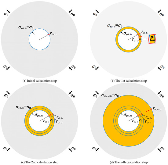
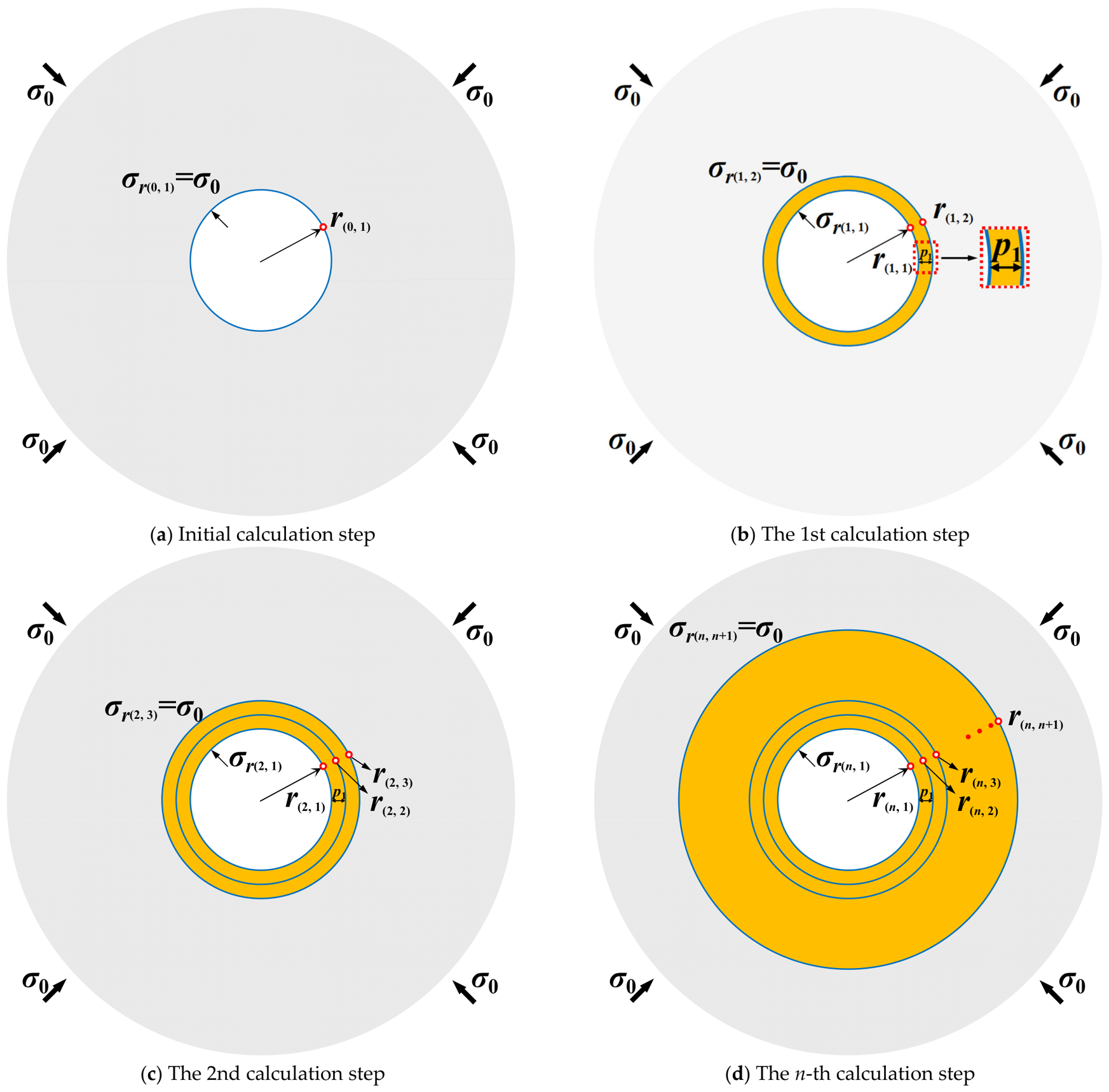
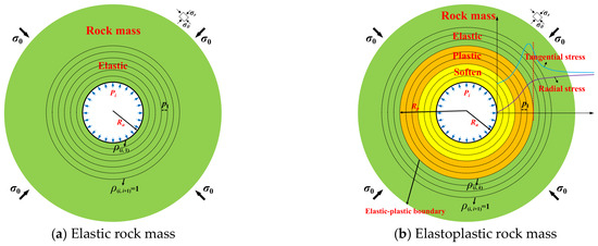
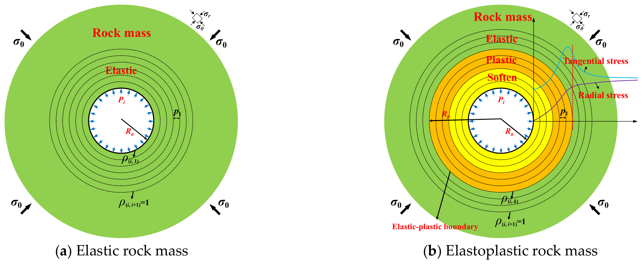
The tunnel construction process is considered a process of n times uniformly releasing radial stress of the rock mass along the tunnel wall (n calculation steps), as shown in Figure 3 [15]. n can be set arbitrarily, with larger values yielding more accurate results, while smaller values may result in less accuracy. In each calculation, the radial stress of p₁ is released along the tunnel wall, and the calculation formula for p₁ is shown in Equation (18). It should be noted that when there is no radial stress release (i.e., the initial calculation step), there is only one initial calculation ring. Subsequently, each release of stress p₁ generates a new calculation ring, with a constant difference in radial stress of p₁ between adjacent rings.

Figure 3. Schematic diagram of a stepwise solution for the rock mass.

Through calculations, the dynamic evolution of rock stress, strain, and displacement throughout the entire construction process can be obtained.

$$p_1={\displaystyle \frac{{\sigma }_0}{n}}$$

(18)

During the calculation process, (i,j) is used to represent the calculation step number and the calculation ring number, where i represents the current calculation step number and j represents the calculation ring number. The numbering of i starts from 0 and proceeds sequentially as 0, 1, 2, …, n. Meanwhile, the numbering of j starts from the innermost ring and gradually increases towards the outer ring. The innermost ring is numbered as 1, and the outermost ring is numbered as i + 1. Thus, the numbering proceeds from the inner to the outer rings as 1, 2, …, i + 1. In the initial calculation step, when i = 0, there is no stress release yet. There is only one initial calculation ring with a numbering of j = 1, located at the inner wall of the tunnel, as shown in Figure 3a. The radial stress σ_r(0,1) at this ring is equal to the initial original rock stress σ₀, while the radius r(0,1) of this ring is equal to the excavation radius R_a of the tunnel. Simultaneously, the radial strain ε_r(0,1), tangential strain ε_θ(0,1), and radial displacement u(0,1) respectively represent the radial deformation, tangential deformation, and radial displacement of this ring. The calculation rings are automatically generated according to a certain pattern. In each new calculation step, a new calculation ring is generated, as shown in Figure 3b–d. Taking the 1st calculation step (i = 1) as an example, as shown in Figure 3b, it includes two calculation rings: one is the calculation ring (1,1) evolved from the existing calculation ring (0,1) at i = 0, and the other is the newly generated calculation ring (1,2) on the outer side of the ring (1,1).

In these two rings, their radial stresses are σ_r(1,1) and σ_r(1,2), respectively, with a radial stress difference in p₁ between them. In each new calculation step, the rings from the previous step gradually contract inward, causing the rock to deform inward toward the tunnel. Meanwhile, a new ring is generated on its outer side, as shown in Figure 3c. Consequently, the stress release zone of the rock gradually extends towards its deeper parts. In the i-th calculation step, the radial stress on the tunnel wall is given by Equation (19).

$${\sigma }_{r\left(i,1\right)}={\sigma }_0-i\times p_1$$

(19)

By computation, the evolution and distribution of radial stress in the rock mass throughout the entire construction process can be obtained. Subsequently, the dynamic evolution laws of parameters such as rock mass strain and displacement can be derived until the completion of construction, i.e., when i = n, as shown in Figure 3d.

3.1. Elastic Solutions

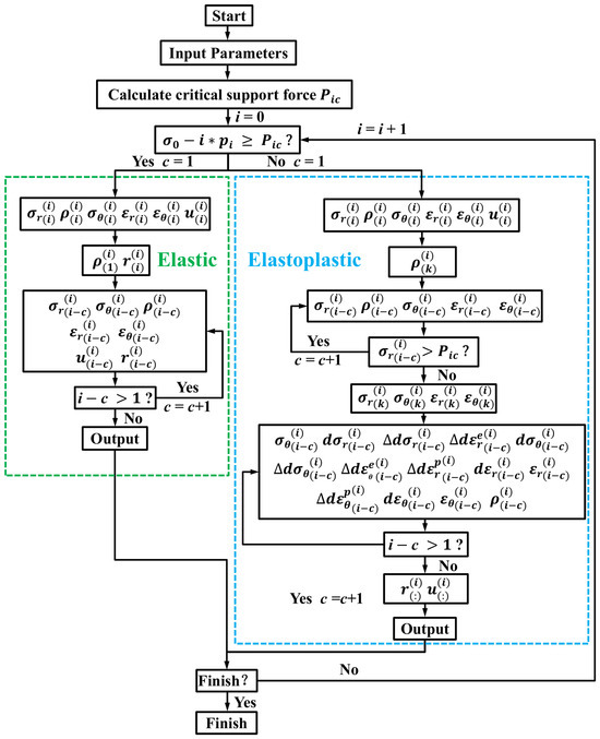
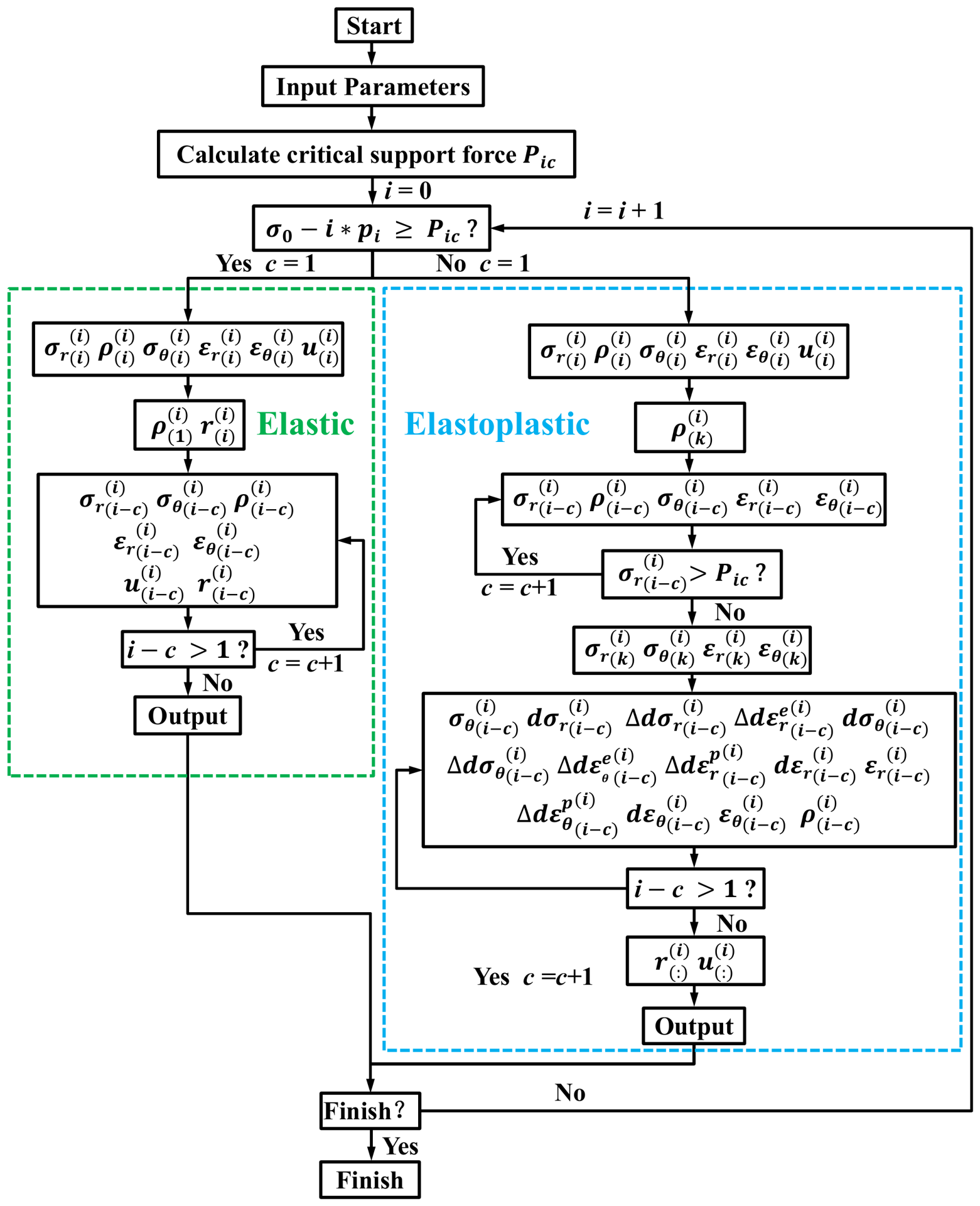
The solution for the elastic zone of the rock mass can be divided into two cases: the solution for the rock mass under purely elastic conditions (Figure 4a) and the solution for the elastic zone of the rock mass under elastic-plastic conditions (Figure 4b). The calculation process for these two cases is similar, with calculations progressing gradually from the outermost ring to the inner rings. Firstly, the calculation results for the outermost ring are obtained, then the results for the next inner ring, and so forth, until reaching the tunnel wall or the elastic-plastic transition zone. Figure 5 illustrates the computational flowchart for the rock mass, where the section enclosed by the green dashed lines represents the process of solving for the elastic rock mass.

Figure 4. Rock mass solution schematic.

Figure 5. Flowchart of rock mass solution.

The calculation method for these two cases is essentially the same. Taking the case of pure elastic rock mass as an example for analysis, Figure 4a illustrates the calculation schematic at the i-th stress release (i-th calculation step). Since the radial stress of the outermost ring is known, i.e., σ_r(i,i + 1) equals the initial stress σ₀, and the radial stress difference p₁ between adjacent rings remains constant, the radial stress of any ring can be easily determined. Calculations are performed using normalized radii, where the normalized radius of the outermost ring, denoted as ρ(i,i + 1), is 1. Here, for ease of calculation, ρ(i,i) is set to 1. In the calculations, since only the ratio between normalized radii is applied, the results are consistent with those obtained directly using radii. By employing the elasticity theory, it is convenient to calculate the normalized radius of the innermost circular ring on the tunnel wall, ρ(i,1), as shown in Equation (20):

$${\rho }_{\left(i,1\right)}={\rho }_{\left(i,i\right)}\sqrt{{\displaystyle \frac{{\sigma }_0-{\sigma }_{r\left(i,i\right)}}{{\sigma }_0-{\sigma }_{r\left(i,1\right)}}}}$$

(20)

During the calculation process, computations proceed sequentially from the outermost circular ring towards the inner rings. When solving for a particular circular ring, the first step is to calculate its normalized radius ρ(i,j), as shown in Equation (21):

$${\rho }_{\left(i,j\right)}=\sqrt{{\displaystyle \frac{\left({\sigma }_0-{\sigma }_{r\left(i,1\right)}\right)}{\left({\sigma }_0-{\sigma }_{r\left(i,j\right)}\right)}}}{\rho }_{\left(i,1\right)}$$

(21)

Then, according to Equations (22)–(25), calculate the tangential stress σ_θ(i,j), radial strain ε_r(i,j), tangential strain ε_θ(i,j), and displacement u(i,j).

$${\sigma }_{\theta \left(i,j\right)}={\sigma }_0+{\displaystyle \frac{{\rho }_{\left(i,1\right)}^2}{{\rho }_{\left(i,j\right)}^2}}\left({\sigma }_0-{\sigma }_{r\left(i,1\right)}\right)$$

(22)

$${\epsilon }_{r\left(i,j\right)}=-{\displaystyle \frac{1}{2G}}{\displaystyle \frac{{\rho }_{\left(i,1\right)}^2}{{\rho }_{\left(i,j\right)}^2}}\left({\sigma }_0-{\sigma }_{r\left(i,1\right)}\right)$$

(23)

$${\epsilon }_{r\left(i,j\right)}={\displaystyle \frac{1}{2G}}{\displaystyle \frac{{\rho }_{\left(i,1\right)}^2}{{\rho }_{\left(i,j\right)}^2}}\left({\sigma }_0-{\sigma }_{r\left(i,1\right)}\right)$$

(24)

$$u_{\left(i,j\right)}={\displaystyle \frac{R_a}{2G}}{\displaystyle \frac{{\rho }_{\left(i,1\right)}}{{\rho }_{\left(i,j\right)}}}\left({\sigma }_0-{\sigma }_{r\left(i,1\right)}\right)$$

(25)

The radius of each ring can be calculated using the following formula:

$$r_{\left(i,j\right)}=R_a{\displaystyle \frac{{\rho }_{\left(i,j\right)}}{{\rho }_{\left(i,1\right)}}}$$

(26)

After calculating each ring sequentially, the stress, strain, radius, and displacement of all calculation rings can be obtained at the i-th stress release step.

When a plastic zone is present, the solution method is similar to that of elastic rock mass, proceeding from the outermost ring towards the inner rings until reaching the elastic-plastic boundary. When the radial stress at the tunnel wall ring is less than the critical support force P_ic, calculations for the plastic zone rings begin.

3.2. Plastic Solutions

After the plastic zone emerges, the solution process follows the right half of Figure 5. Assuming the k-th ring is the elastic-plastic boundary, based on elastoplastic theory, the stress and strain at the elastic-plastic boundary can be readily calculated as shown in Equations (27)–(30):

$${\sigma }_{r_{\left(i,k\right)}}=P_{ic}$$

(27)

$${\sigma }_{{\theta }_{\left(i,k\right)}}=2{\sigma }_0-P_{ic}$$

(28)

$${\epsilon }_{r_{\left(i,k\right)}}={\displaystyle \frac{P_{ic}-{\sigma }_0}{2G}}$$

(29)

$${\epsilon }_{{\theta }_{\left(i,k\right)}}={\displaystyle \frac{{\sigma }_0-P_{ic}}{2G}}$$

(30)

By solving the equilibrium differential equations, Equation (31) can be obtained:

$${\displaystyle \frac{{\sigma }_{r\left(i,j+1\right)}-{\sigma }_{r\left(i,j\right)}}{r_{\left(i-1,j+1\right)}-r_{\left(i-1,j\right)}}}+{\displaystyle \frac{{\sigma }_{r\left(i,j\right)}-{\sigma }_{\theta \left(i,j\right)}}{r_{\left(i-1,j\right)}}}=0$$

(31)

Since the result of ρ(i,j) is unknown in the current calculation step, the same numbered circle ρ(i − 1,j) from the previous calculation step is used as the initial value for ρ(i,j) in the current calculation step. Although some errors may occur during the calculation process, as long as p₁ is small enough, meaning a sufficient number of circles are involved in the calculation, the computational errors caused by each circle will be very small and can be negligible.

From Equation (31), it can be inferred that the tangential stress σ_θ(i,j) of the j-th circle can be expressed in terms of the radial stresses σ_r(i,j) and σ_r(i,j + 1) as shown in Equation (32):

$${\sigma }_{\theta \left(i,j\right)}={\sigma }_{r\left(i,j\right)}+{\displaystyle \frac{{\sigma }_{r\left(i,j+1\right)}-{\sigma }_{r\left(i,j\right)}}{r_{\left(i-1,j+1\right)}-r_{\left(i-1,j\right)}}}{\rho }_{\left(i-1,j\right)}$$

(32)

In the i-th calculation step, the current strain ε(i,j) of the rock mass can be expressed as the sum of the strain in the (i − 1)-th calculation step ε(i − 1,j) and the incremental strain dε(i,j) in the i-th calculation step, as follows:

$$\left\{\begin{array}{l}{\epsilon }_{r\left(i,j\right)}={\epsilon }_{r\left(i-1,j\right)}+d{\epsilon }_{r\left(i,j\right)}\hfill \\ {\epsilon }_{\theta \left(i,j\right)}={\epsilon }_{\theta \left(i-1,j\right)}+d{\epsilon }_{\theta \left(i,j\right)}\hfill \end{array}\right.$$

(33)

In the above equation, dε_r(i,j) and dε_θ(i,j) represent the incremental radial strain and tangential strain, respectively, of the j-th ring in the i-th calculation step. For the ring located at the elastic-plastic boundary (the k-th ring), the radial strain ε_r(i,k) and tangential strain ε_θ(i,k) are known. For other circles (1 ≤ j ≤ k), the strain components dε_r(i,j) and dε_θ(i,j) can be obtained by using the results of their outer adjacent circles. For any given circle j, the strain increment dε(i,j) consists of the following components: the strain increment dε(i,j + 1) of the j + 1 circle, the increase in radial strain increment ∆dε^e(i,j) of circle j, and the increase in tangential strain increment ∆dε^p(i,j), as shown in the following equation:

$$\left\{\begin{array}{l}d{\epsilon }_{r\left(i,j\right)}=d{\epsilon }_{r\left(i,j+1\right)}+\Delta d{\epsilon }_{r\left(i,j\right)}^e+\Delta d{\epsilon }_{r\left(i,j\right)}^p\hfill \\ d{\epsilon }_{\theta \left(i,j\right)}=d{\epsilon }_{\theta \left(i,j+1\right)}+\Delta d{\epsilon }_{\theta \left(i,j\right)}^e+\Delta d{\epsilon }_{\theta \left(i,j\right)}^p\hfill \end{array}\right.$$

(34)

In the equation above, the subscripts r and θ represent the radial and tangential directions, respectively. Here, ∆dε^e(i,j) and ∆dε^p(i,j) represent the increase in strain increments of the j-th ring in the i-th calculation step, indicating the difference between the strain increments in the i-th and (i − 1)-th calculation steps. ∆dε_{e r}(i,j) represents the increase in radial elastic strain increment, ∆dε_{p r}(i,j) represents the increase in radial plastic strain increment, ∆${d\epsilon }_{\theta }^p$(i,j) represents the increase in tangential elastic strain increment, and ∆${d\epsilon }_{\theta }^p$(i,j) represents the increase in tangential plastic strain increment. ∆dε_{e r}(i,j) and ∆${d\epsilon }_{\theta }^p$(i,j) are calculated using Hooke’s law, as shown in the following equations:

$$\left[\begin{array}{l}\Delta d{\epsilon }_{r\left(i,j\right)}^e\hfill \\ \Delta d{\epsilon }_{\theta \left(i,j\right)}^e\hfill \end{array}\right]={\displaystyle \frac{1}{2G}}\left[\begin{array}{cc}1-v& -v\\ -v& 1-v\end{array}\right]\left[\begin{array}{c}\Delta d{\sigma }_{r\left(i,j\right)}\\ \Delta d{\sigma }_{\theta \left(i,j\right)}\end{array}\right]$$

(35)

The increase in radial stress increment ∆dσ_r(i,j) and the increase in tangential stress increment ∆dσ_θ(i,j) for the j-th ring are calculated as follows.

$$\begin{array}{c}\Delta d{\sigma }_{r\left(i,j\right)}=d{\sigma }_{r\left(i,j\right)}-d{\sigma }_{r\left(i,j+1\right)}\\ \Delta d{\sigma }_{\theta \left(i,j\right)}=d{\sigma }_{\theta \left(i,j\right)}-d{\sigma }_{\theta \left(i,j+1\right)}\end{array}$$

(36)

dσ_r(i,j) and dσ_θ(i,j) represent the increments of radial stress and tangential stress for the j-th ring, respectively. The calculation formulas are as follows:

$$\begin{array}{c}d{\sigma }_{r\left(i,j\right)}={\sigma }_{r\left(i,j\right)}-{\sigma }_{r\left(i-1,j\right)}\\ d{\sigma }_{\theta \left(i,j\right)}={\sigma }_{\theta \left(i,j\right)}-{\sigma }_{\theta \left(i-1,j\right)}\end{array}$$

(37)

Assuming that the increments of plastic strain components satisfy the non-associated flow rule:

$$d{\epsilon }_{r\left(i,j\right)}^p+k_{\left(i\right)}d{\epsilon }_{\theta \left(i,j\right)}^p=0$$

(38)

$$k_{\left(i\right)}={\displaystyle \frac{1+\sin {\varphi }_{\left(i\right)}}{1-\sin {\varphi }_{\left(i\right)}}}$$

(39)

In the above equation, ϕ(i) represents the dilation angle of the rock mass.

The total strain increments dε_r(i,j) and dε_θ(i,j) need to satisfy the following equations:

$${\displaystyle \frac{d{\epsilon }_{\theta \left(i,j\right)}-d{\epsilon }_{\theta \left(i,j+1\right)}}{r_{\left(i-1,j\right)}-r_{\left(i-1,j+1\right)}}}+{\displaystyle \frac{d{\epsilon }_{\theta \left(i,j\right)}-d{\epsilon }_{r\left(i,j\right)}}{r_{\left(i-1,j\right)}}}=0$$

(40)

Expressing the total strain increment dε(i,j) as the sum of plastic strain increment dε^p(i,j) and elastic strain increment dε^e(i,j), the components of plastic strain increment can be expressed as:

$$d{\epsilon }_{\theta \left(i,j\right)}^p={\displaystyle \frac{\frac{d{\epsilon }_{\theta \left(i,j+1\right)}^p-d{\epsilon }_{\theta \left(i,j\right)}^e+d{\epsilon }_{\theta \left(i,j+1\right)}^e}{r_{\left(i-1,j\right)}-r_{\left(i-1,j+1\right)}}-2\frac{d{\epsilon }_{\theta \left(i,j\right)}^e+d{\epsilon }_{r\left(i,j\right)}^e}{r_{\left(i-1,j\right)}+r_{\left(i-1,j+1\right)}}}{\frac{1}{r_{\left(i-1,j\right)}-r_{\left(i-1,j+1\right)}}-\frac{2+2k_{\left(i\right)}}{r_{\left(i-1,j\right)}+r_{\left(i-1,j+1\right)}}}}$$

(41)

$$d{\epsilon }_{r\left(i,j\right)}^p=-k_{\left(i\right)}d{\epsilon }_{\theta \left(i,j\right)}^p$$

(42)

The difference in plastic strain increments between the inner and outer sides of the j-th ring, ∆dε^p(i,j), is:

$$\Delta d{\epsilon }_{r\left(i,j\right)}^p=d{\epsilon }_{r\left(i,j\right)}^p-d{\epsilon }_{r\left(i,j+1\right)}^p$$

(43)

$$\Delta d{\epsilon }_{\theta \left(i,j\right)}^p=d{\epsilon }_{\theta \left(i,j\right)}^p-d{\epsilon }_{\theta \left(i,j+1\right)}^p$$

(44)

The radial and tangential strains, ε_r(i,j) and ε_θ(i,j), of each ring in the i-th calculation step can be obtained through computation.

From the yield function, H(i,j) can be obtained.

$$H_{\left(i,j\right)}={\sigma }_{\theta \left(i,j\right)}-{\sigma }_{r\left(i,j\right)}$$

(45)

The calculation formula for the normalized radius ρ(i,j) is as follows:

$${\rho }_{\left(i,j\right)}={\rho }_{\left(i-1,j\right)}{\displaystyle \frac{2H_{\left(i,j\right)}+\Delta {\sigma }_{r\left(i,j\right)}}{2H_{\left(i,j\right)}-\Delta {\sigma }_{r\left(i,j\right)}}}$$

(46)

The radius of each ring is given by the following equation:

$$r_{\left(i,j\right)}=R_a{\displaystyle \frac{{\rho }_{\left(i,j\right)}}{{\rho }_{\left(i,1\right)}}}$$

(47)

The displacement of each ring is given by the following equation:

$$u_{\left(i,j\right)}=r_{\left(i,j\right)}{\epsilon }_{\theta \left(i,j\right)}$$

(48)

4. Solutions for the Supported Tunnels

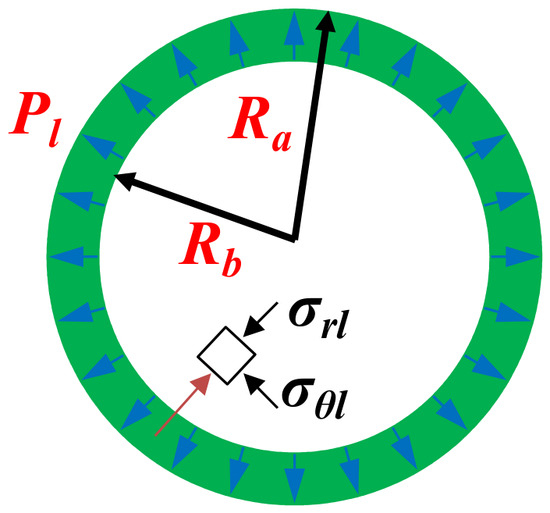
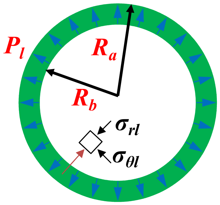
This study takes lining as an example for analysis, as shown in Figure 6. Based on the fundamental theory of thick-walled cylinders and considering the stress boundary conditions of the lining, stress and displacement solutions for the lining can be derived [26].

$$\left\{\begin{array}{l}{P}_l=K_l{u}_l={\displaystyle \frac{E_l\left({R_a}^2-{R_b}^2\right)r}{\left(1+{\nu }_l\right)\left(\left(1-2{\nu }_l\right)r^2+{R_b}^2\right)}}{u}_l\hfill \\ {\sigma }_{rl}={\displaystyle \frac{{R_a}^2\left(r^2-{R_b}^2\right)P_l}{\left({R_b}^2-{R_a}^2\right)r^2}}\hfill \\ {\sigma }_{\theta l}={\displaystyle \frac{{R_a}^2\left(r^2+{R_b}^2\right)P_l}{\left({R_b}^2-{R_a}^2\right)r^2}}\hfill \end{array}\right.$$

(49)

Figure 6. Schematic diagram of thick-walled cylinder theory.

In Equation (49), P_l, K_l, u_l, E_l, v_l, σ_rl, and σ_θl respectively represent the support force, stiffness, radial displacement, elastic modulus, Poisson’s ratio, radial stress, and tangential stress of the lining. r represents the radius.

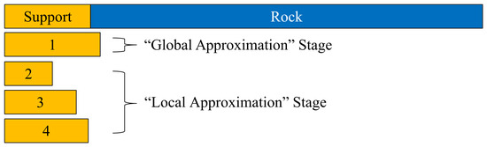
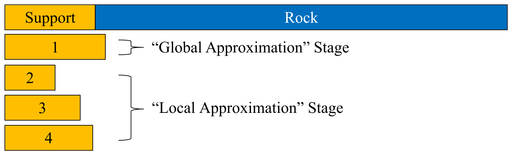
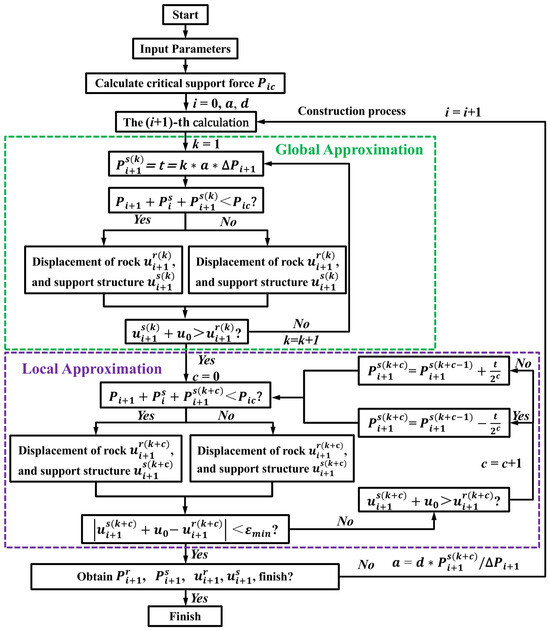
Consistent with previous studies [26,27], it is known that the rock mass bears the majority of the load, while the support bears a small portion of it. Based on this conclusion and drawing inspiration from the ISLM solution approach [21], this study proposes an iterative calculation method called the Support Load Approximation Strategy (SLAS) to solve the cooperative bearing process of the rock-support system. The methodology is illustrated in Figure 7.

Figure 7. Solution schematic diagram of Support Load Approximation Strategy (SLAS).

SLAS consists of two stages: the “Global Approximation” stage and the “Local Approximation” stage. The purpose of the “Global Approximation” stage is to approximate (slightly greater than) the actual load borne by the support. The purpose of the “Local Approximation” stage is to progressively approach the load obtained from the “Global Approximation” using a binary search method. The solution diagram of SLAS is illustrated in Figure 8.

Figure 8. Flowchart of Support Load Approximation Strategy (SLAS).

Assuming that after the i-th calculation, the load borne by the support is $P_i^s$, the load borne by the rock mass is $P_i^r$, the virtual support force provided by the lining is P_i, the displacement of the support is $u_i^s$, and the displacement of the rock mass is $u_i^r$. At the time of support application, the displacement of the rock mass is u₀, thus $u_i^s$ equals $u_i^r$ − u₀. At the end of the (i + 1)-th calculation, the virtual support force at the heading face decreases from P_i to P_i+1, and the reduced load is denoted as ∆P_i+1. ∆P_i+1 will be shared by both the rock mass and the support. In the (i + 1)-th calculation, the main focus is on determining the allocation of the load ∆P_i+1. $P_{{s\left(k\right)}_{i+1}}$ represents the additional load borne by the support in the (i + 1)-th calculation, where k denotes the trial number. ∆P_i+1 − $P_{{s\left(k\right)}_{i+1}}$ represents the additional load borne by the rock mass in the (i + 1)-th calculation. During the entire construction process, the virtual support force at the heading face will decrease from the original rock stress σ₀ to 0. In the calculation process of the (i + 1)-th rock stress release, the following two steps can be followed:

Global Approximation: Initially, in the early stage of the calculation, the “Global Approximation” phase is conducted. During this phase, the support is incrementally loaded by a certain percentage, denoted as a% ∗ ∆P_i+1, ensuring that the calculated displacement of the support is slightly larger than that of the rock mass. Generally, this process only needs to be calculated once.

At i = 0, the initial value of a is set arbitrarily, typically between 0.2 and 0.5. In subsequent calculations, the value of a is obtained from the calculation. For example, in the (i + 1)th calculation, the value of a is ($P_{i+1}^{s\left(k\right)}$/∆P_i+1) ∗ d from the i-th calculation, aiming to make $P_{i+1}^{s\left(k\right)}$ slightly larger than the actual result, so that the global approximation phase only needs to be calculated once. We have conducted numerous computational studies, and the coefficient d performs better when set to 1.1 or 1.2.

Local Approximation: Subsequently, the ‘Local Approximation’ stage of computation is performed. In this stage, binary search is employed to compute the bearing capacity of the support, ensuring that the absolute difference between the relative displacement of the rock mass $u_{i+1}^r$ − u₀ and the displacement of the support $u_{i+1}^s$ is essentially the same, i.e., less than a very small value ε_min.

The proportion of load borne by the support is relatively small, typically not exceeding 20% of the total load. In some studies, the load borne by the support is even smaller, around 1% [26]. Therefore, the calculation range of the “local approximation” stage is usually between 1% and 20% of ∆P_i+1. After the (i + 1)-th calculation, we obtain the load borne by the rock mass, $P_{i+1}^r$, and its displacement, $u_{i+1}^r$, as well as the load borne by the support, $P_{i+1}^s$, and its displacement, $u_{i+1}^s$.

5. Verification Examples

To validate the accuracy of the algorithm proposed in this study, two examples are used to verify the research content of Section 3 and Section 4. The research described above has been implemented in Matlab code. Example 1 involves a comparative analysis with traditional theoretical results, while Example 2 involves a comparative analysis with the computational results from the Flac3D finite difference program.

5.1. Example 1

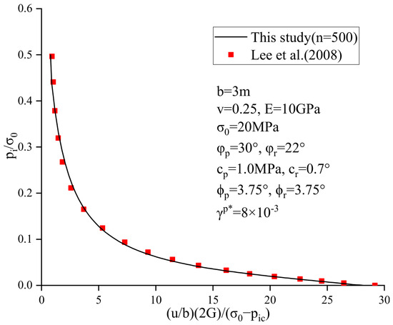
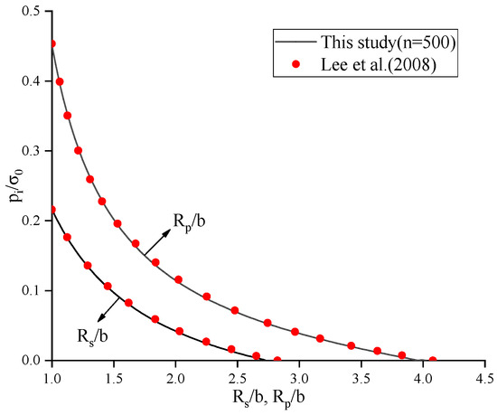
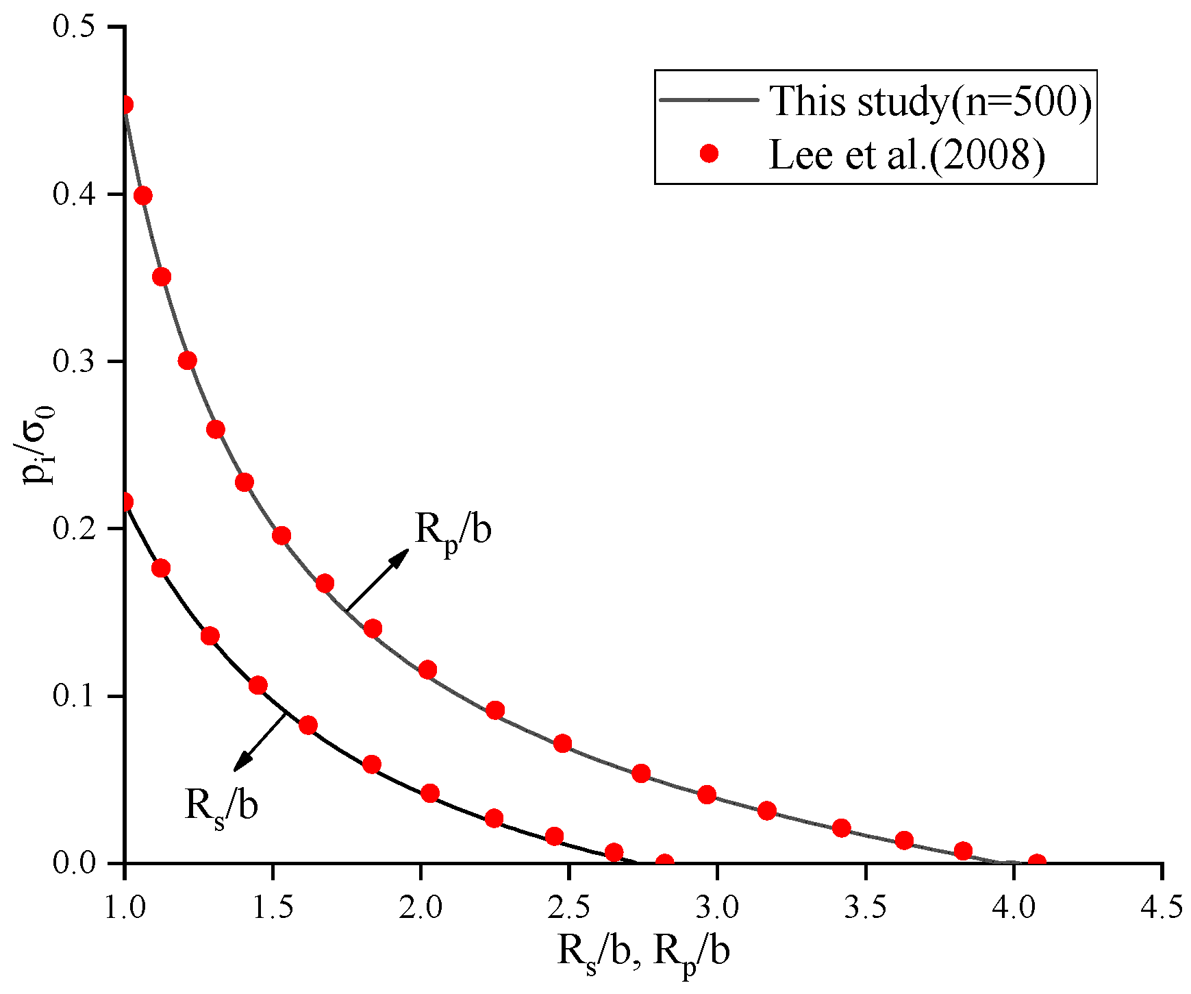
Lee et al. (2008) [1] proposed a series of strain-softening solutions for circular tunnels using the finite difference method. The data reported in Lee et al. (2008) [1] are employed to validate the accuracy of the algorithm presented in this paper. The number of calculation steps, n, is set to 100. The GRC of the MC strain-softened rock mass is shown in Figure 9, and the plastic zone radius R_p and softening radius R_s are illustrated in Figure 10.

Figure 9. GRC for a strain-softening M–C rock mass (adapted from Lee et al. (2008) [1]).

Figure 10. Evolution plastic radii in a strain-softening M–C rock mass (adapted from Lee et al. (2008) [1]).

The GRC and plastic radii (Rp and Rs) curves obtained by the proposed method agree excellently with the results of Lee et al. (2008) [1], showing a very high degree of curve shape similarity and excellent overall consistency. Quantitative comparisons show that the relative errors are 3.73% for the GRC, 1.47% for R_s, and 3.40% for R_p, confirming the correctness and accuracy of the proposed algorithm.

5.2. Example 2

The mechanical parameters of the rock mass in this example, which adopts the MC criterion, are as follows: E = 4 GPa, v = 0.25, φ_p = 33°, φ_r = 22°, c_p = 1.6 MPa, c_r = 1.0 MPa, ϕ_p = 3.75°, ϕ_r = 3.75°, γ^p = 0.008. The elastic modulus of the lining is 30 GPa, Poisson’s ratio is 0.2, and the thickness is 0.5 m, modeled as linear elastic.

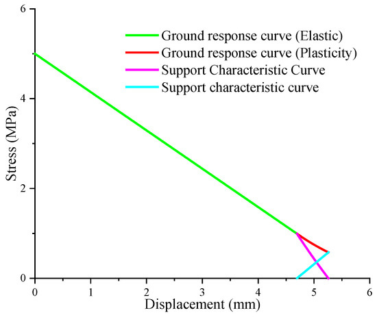
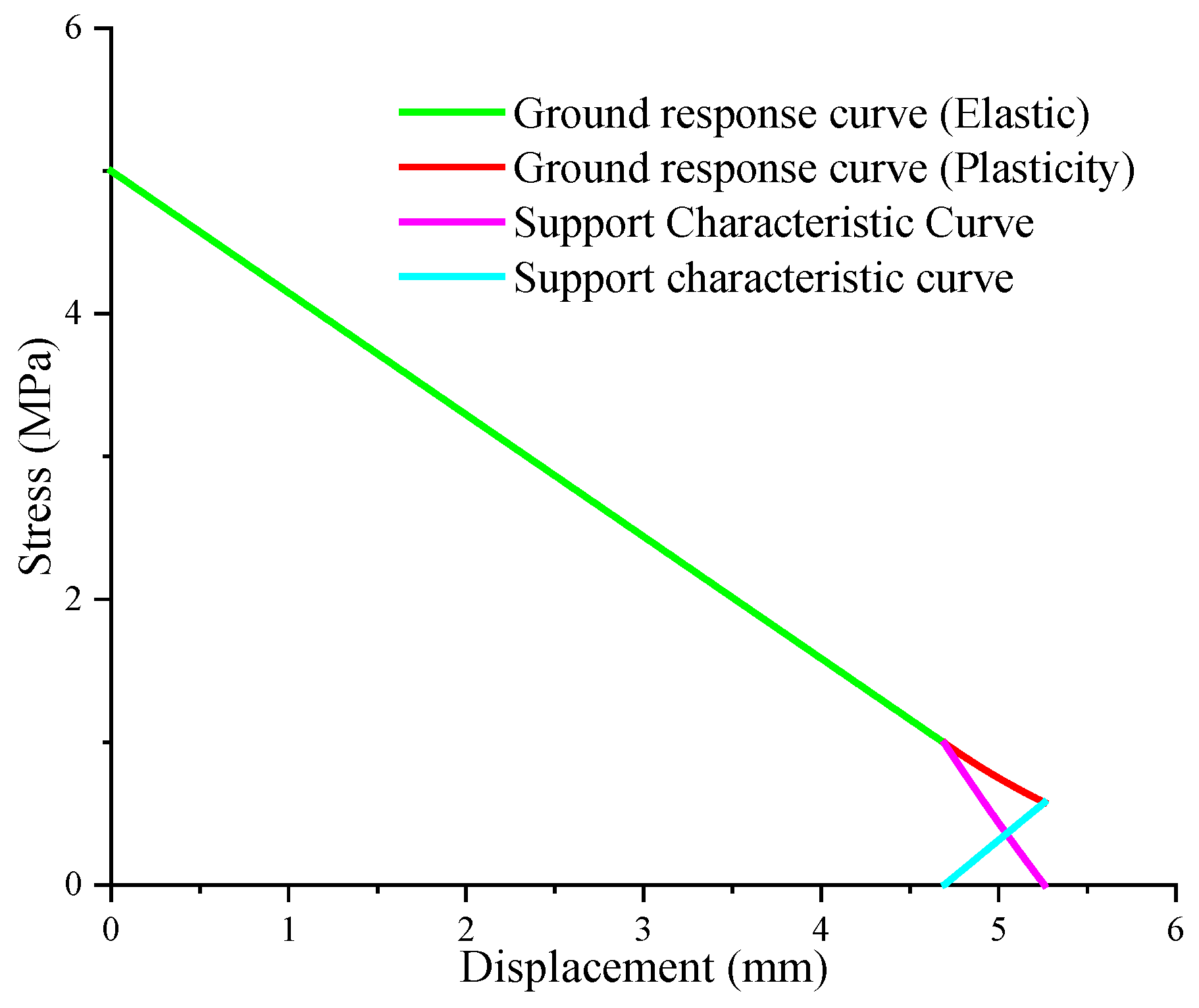
The tunnel radius b is 3.75 m, and the initial stress σ₀ is 5.0 MPa. A stress release rate of 0.8 is assumed during lining installation. The collaborative load-bearing process of the rock-lining system is illustrated in Figure 11.

Figure 11. The collaborative load-bearing process of the rock-lining system.

The green and red curves in the figure represent the GRC in the purely elastic state and after the occurrence of the plastic zone, respectively. The magenta curve represents the virtual support force curve, and the cyan curve represents the lining support force curve. After reaching a stable state, the displacement of the rock mass is 5.26 mm, and the lining support force is 0.58 MPa.

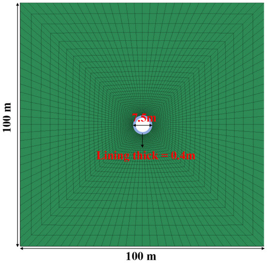
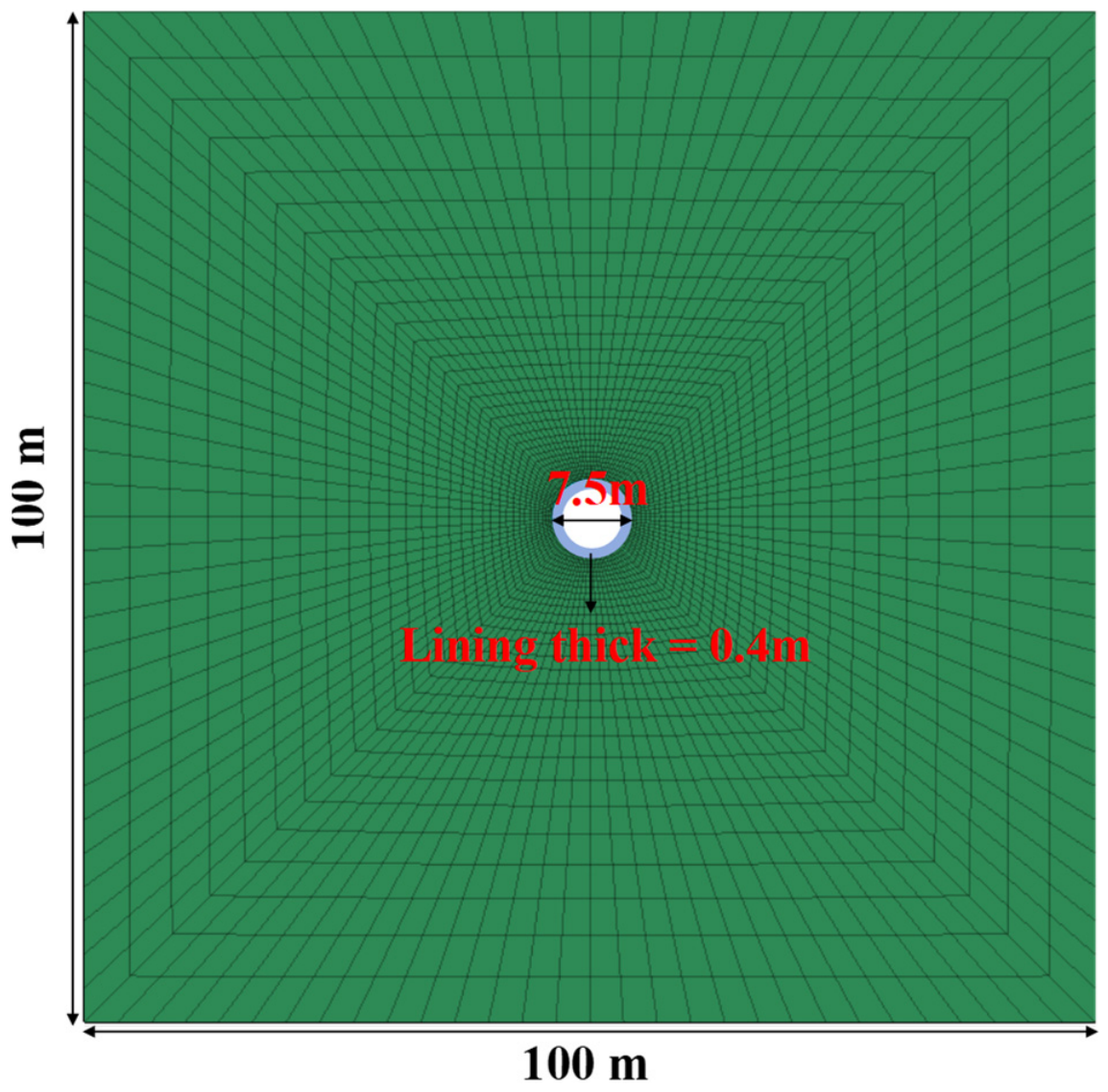
Figure 12 depicts a numerical model with a thickness of 5 m along the axis of the tunnel. The front and rear faces of the model are subjected to normal constraints, so it can be considered as a plane strain problem. Other boundary conditions and computational parameters in the numerical model are consistent with those in the theoretical model.

Figure 12. Numerical model mesh for Flac3D simulation.

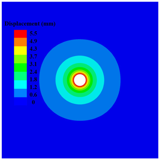
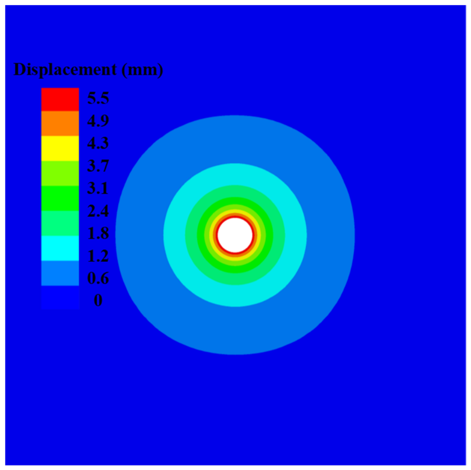
Figure 13 shows the numerical calculation results of rock mass displacement. The theoretical displacement is 5.26 mm, while the numerical displacement is 5.5 mm. The two values are very close, with a maximum error of less than ±5%. The discrepancy is attributed to the differences in element size around the tunnel in the numerical model.

Figure 13. Rock displacement.

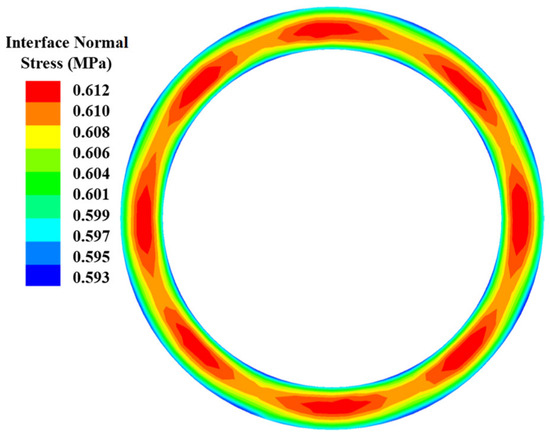
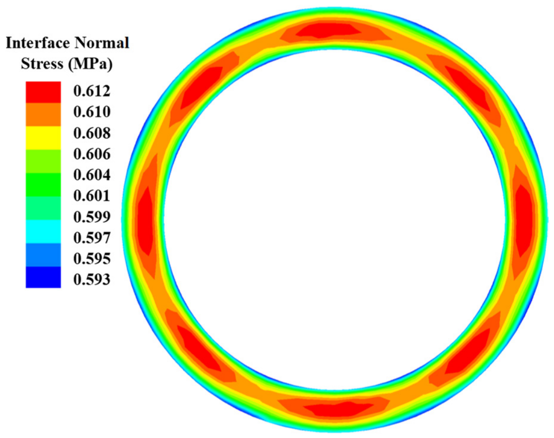
Figure 14 depicts the normal stresses obtained from the numerical simulation of the lining interface (support force of the lining). It can be observed that the normal stresses along the periphery of the tunnel interface are nearly uniform, confirming the feasibility of using interface elements to simulate the contact behavior between the rock mass and the lining. The normal stress on the interface is approximately 0.61 MPa, which is approximately equal to the theoretical value of the lining support force.

Figure 14. Lining normal stress.

The above study shows that theoretical calculations are consistent with numerical simulation results.

6. Analysis and Discussion

6.1. Analysis of Computational Accuracy

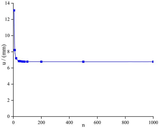
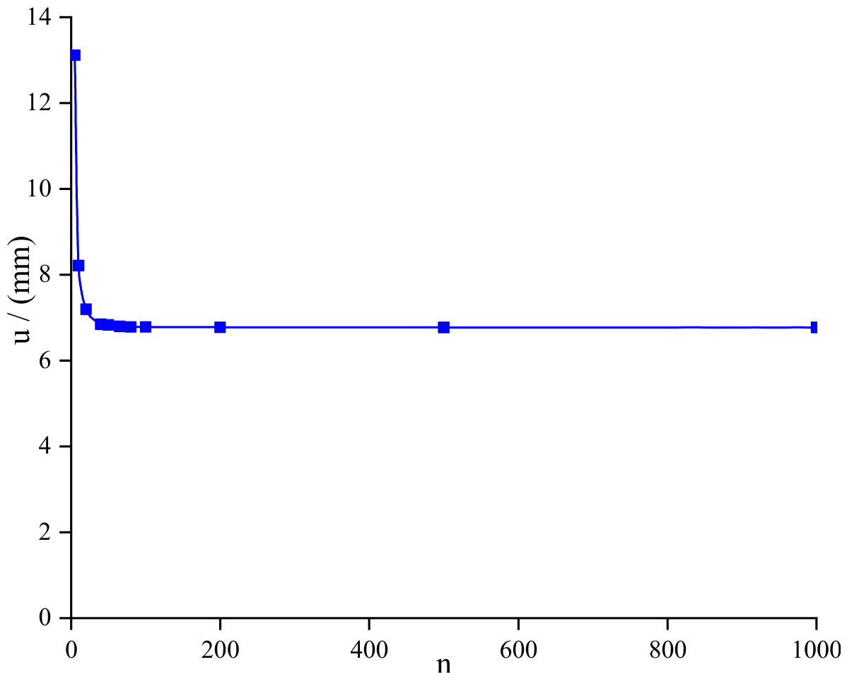
The calculation in the current step is based on the results of the previous step, not the current one, which may introduce errors in the computation. In theory, if the number of rings n involved in the calculation is large enough, meaning that the released radial stresses in each new calculation step are relatively small, the error will be smaller. Therefore, there is a relationship between the number of calculation rings and the calculation accuracy. If the total number of calculation steps n is large enough, the calculation error will be smaller, but the calculation time will greatly increase. To determine the appropriate n, this analysis focuses on the relationship between the total number of calculation steps n and the maximum displacement of the rock mass during tunnel excavation. This serves as an example to explore how n affects the maximum displacement of the rock mass. The mechanical parameters of the rock mass are consistent with those of Case 2, without considering the support. The range of variation for n is taken as 5 to 1000. The relationship between the calculated maximum displacement of the rock mass and n is shown in Figure 15.

Figure 15. Relationship between n and tunnel displacement.

As shown in Figure 15, the displacement at n = 40 is 6.847 mm. When n increases to 200, 500, and 1000, the displacements are 6.775 mm, 6.772 mm, and 6.770 mm, respectively. Compared to n = 40, the percentage differences are only −1.05%, −1.10%, and −1.12%, respectively. Furthermore, compared to n = 200, the differences at n = 500 and n = 1000 are only −0.04% and −0.07%, respectively, indicating that the results have already converged well at n = 200. Therefore, to significantly improve computational efficiency while maintaining sufficient accuracy, the recommended range for n is 40 to 200.

6.2. Comparison with Traditional Methods

6.2.1. Rock Solution Method

The solution approach in this study is quite similar to that proposed by Lee et al. (2008) [1], with the following differences:

(1)

In Lee’s method [1], the number of rings involved in the plastic zone calculation remains constant at a certain value k and does not change with variations in the plastic zone. As is well-known, the extent of the plastic zone gradually increases, and the degree of deterioration of the plastic rock deepens over time. Therefore, in the initial stages of calculation, when the plastic zone is small, excessive calculation of the number of rings may lead to wastage of computational resources. Conversely, in the later stages, an insufficient number of calculation rings may result in a decrease in computational accuracy. In contrast, in the algorithm proposed in this paper, the number of rings involved in the calculation increases with the expansion of the plastic zone, which is more conducive to the efficient utilization of computational resources. Advancements in scientific research are built on gradual accumulation. The improvement of this method provides insights for the elastic-plastic analysis of the surrounding rock and contributes to the development of efficient computational methods in other fields.

(2)

Xu et al. (2021) [23] made improvements to Lee’s method [1], and their revised method is also quite clever. But in the i-th calculation after the onset of the plastic zone, we need the radius r(i − 1,i + 1) obtained from the (i − 1)-th calculation. However, in the (i − 1)-th calculation, only r(i − 1,1) − r(i − 1,i) exists, and r(i − 1,i + 1) does not exist. Therefore, in the i-th calculation, it is necessary to make certain assumptions to obtain r(i − 1,i + 1), which increases the difficulty of understanding and the complexity of the calculation. In this study, r(i − 1,i + 1) obtained from the previous calculation step can be conveniently used.

(3)

In this study, it was found that initiating the calculation from the outermost ring and proceeding inward is not feasible. For instance, the normalized radius of the outermost ring is ρ(k,k + 1) = 1, and its radial stress σ_r(i,i + 1) equals the initial stress σ₀. Substituting the outermost ring into Equation (20) would give σ₀ − σ_r(i,i + 1) = 0, leading to ρ(k,1) = 0 and making further calculations impossible. To address this issue, this study proposes using the second-to-last ring ρ(k,k) as the starting point for calculations, where the corresponding radial stress is σ_r(i,i) and σ_r(i,i) ≠ σ₀. As long as a sufficient number of rings are involved in the calculation, the resulting error is negligible.

6.2.2. Rock-Support System Solution Method

All comparisons presented in this section were carried out under the same hardware and software conditions (same computer with identical CPU, memory, and MATLAB environment) to ensure a fair evaluation of algorithmic performance.

In the SLAS, typically, the “Global Approximation” phase only needs to be computed once before the “Local Approximation” phase can be initiated. The “Local Approximation” phase usually requires no more than 10 computations. The SLAS offers advantages in both computational efficiency and accuracy compared to traditional binary search methods and the ISLM. As an example, in the i-th calculation, suppose the stress released by the rock mass is 100,000 Pa. When the load borne by the support reaches 9050 Pa, and the difference between the relative displacements of the support and the rock mass is less than a very small constant ε_min, stability is achieved.

If the ISLM is used, with an increment of 100 Pa each time, it requires 91 iterations, resulting in an error of 50 Pa. With the binary search method, 10 iterations are needed, with an error of 32 Pa. However, when d is set to 1.1, SLAS requires fewer than six iterations, with an error of less than 15 Pa. Compared to ISLM, SLAS improves computational efficiency by 14.2 times and accuracy by 70%. Compared to the binary search method, SLAS improves computational efficiency by 0.67 times and accuracy by 53%. To improve computational accuracy, the stress increment is set to 9 Pa. In this case, ISLM requires 1006 calculations with an error of 4 Pa, while the binary search method requires 14 calculations with an error of 1.5 Pa. Meanwhile, SLAS requires fewer than 11 calculations with an error of less than 3 Pa. Compared to ISLM and binary search, while maintaining similar computational accuracy, SLAS’s computational efficiency has increased by 82.8 and 0.17 times, respectively.

From these examples, it can be seen that SLAS outperforms ISLM and binary search in terms of computational efficiency and accuracy. This demonstrates the superiority of the SLAS, which can obtain calculation results more quickly and accurately.

7. Conclusions

(1)

A novel elastoplastic analysis method is proposed for circular tunnels during construction, considering rock strain softening. This method uses the “second-to-last ring” instead of the “outermost ring” for calculations, simplifying the computational process and reducing the difficulty of understanding. Validation against the theoretical results of Lee et al. (2008) [1] demonstrates that the ground reaction curve (GRC) and the plastic radii (R_p and R_s) curves obtained by the proposed method are in excellent agreement with the literature, showing a very high degree of similarity in curve shapes. The relative errors are 3.73% for the GRC, 1.47% for R_s, and 3.40% for R_p, confirming the correctness and accuracy of the proposed algorithm.

(2)

To address the challenge of lacking closed-form analytical solutions for the theory model of rock-supporting system cooperative bearing, a method called “Support Load Approximation Strategy” (SLAS) is proposed as an iterative computational approach. This method can ascertain the loads borne by both the rock mass and support and can also elucidate the cooperative evolution of the rock-support system during tunnel construction. The reasonableness of SLAS has been validated through numerical examples.

(3)

SLAS exploits the characteristic that the rock mass bears the majority of the load while the support bears a smaller portion, thereby achieving both high computational efficiency and accuracy. The examples demonstrate that, with a stress increment of 100 Pa per step, SLAS improves computational efficiency by 14.2 times and 0.7 times, and accuracy by 74% and 38%, respectively, compared to ISLM and the binary search method.

References

- Lee, Y.K.; Pietruszczak, S. A new numerical procedure for elasto-plastic analysis of a circular opening excavated in a strain-softening rock mass. Tunn. Undergr. Space Technol. 2008, 23, 588–599. [Google Scholar] [CrossRef] [Scilit]
- Yu, S.; Ren, X.; Zhang, J.; Sun, Z. Numerical simulation on the excavation damage of Jinping deep tunnels based on the SPH method. Geomech. Geophys. Geo-Energy Geo-Resour. 2023, 9, 1. [Google Scholar] [CrossRef] [Scilit]
- Zhang, Z.; Dias, D.; Anitescu, C.; Pan, Q.; Rabczuk, T. Physics-informed neural network for elastic–plastic mesh-free modelling of tunnelling-induced deformation. Acta Geotech. 2026, 21, 349–370. [Google Scholar]
- Li, X.; Sun, R.; Yang, Y.; Chen, S. Dual-Shaking Table Test of Fault-Crossing Tunnel Structure Model and Rationality Analysis of Seismic Action Modes. Symmetry 2026, 18, 890. [Google Scholar] [CrossRef] [Scilit]
- Zhu, G.; Li, S.; Li, C.; Liu, G.; Zhou, Y. Physical Model Study on Brittle Failure of Pressurized Deep Tunnel with Support System. Rock Mech. Rock Eng. 2023, 56, 9013–9033. [Google Scholar] [CrossRef] [Scilit]
- Zhang, Z.; Pan, Q.; Yang, Z.; Yang, X. Physics-informed deep learning method for predicting tunnelling-induced ground deformations. Acta Geotech. 2023, 18, 4957–4972. [Google Scholar] [CrossRef] [Scilit]
- Yu, S.; Ren, X.; Zhang, J. Modeling the rock frost cracking processes using an improved ice–Stress–Damage coupling method. Theor. Appl. Fract. Mech. 2024, 131, 104421. [Google Scholar] [CrossRef] [Scilit]
- Sun, Z.; Zhang, D.; Fang, Q.; Liu, D.; Dui, G. Displacement process analysis of deep tunnels with grouted rockbolts considering bolt installation time and bolt length. Comput. Geotech. 2021, 140, 104437. [Google Scholar] [CrossRef] [Scilit]
- Fairhurst, C.T. Application of the Convergence-Confinement method of tunnel design to rock masses that satisfy the Hoek-Brown failure criterion. Tunn. Undergr. Space Technol. 2000, 15, 187–213. [Google Scholar] [CrossRef] [Scilit]
- Li, S.-c.; Wang, M.-b. An elastic stress–displacement solution for a lined tunnel at great depth. Int. J. Rock Mech. Min. Sci. 2008, 45, 486–494. [Google Scholar] [CrossRef] [Scilit]
- Sharan, S.K. Exact and approximate solutions for displacements around circular openings in elastic–brittle–plastic Hoek–Brown rock. Int. J. Rock Mech. Min. Sci. 2005, 42, 542–549. [Google Scholar] [CrossRef] [Scilit]
- Chen, Y.; Binti Jusoh, S.N.; Abdullah, R.A.B.; Ahmad Shah, M.S.B.; Zhang, B.; Li, J.; Liu, C.; Lu, Z.; Wang, L. Deformation Control and Structural Performance of a Double- Sidewall Pilot Tunnelling Method with Reserved Rock Walls: A Case Study of a Large-Span Tunnel in Grade V Weak Rock. Buildings 2026, 16, 2079. [Google Scholar] [CrossRef] [Scilit]
- Zhang, Q.; Jiang, B.S.; Wang, S.L.; Ge, X.R.; Zhang, H.Q. Elasto-plastic analysis of a circular opening in strain-softening rock mass. Int. J. Rock Mech. Min. Sci. 2012, 50, 38–46. [Google Scholar] [CrossRef] [Scilit]
- Cui, L.; Zheng, J.J.; Zhang, R.J.; Dong, Y.K. Elasto-plastic analysis of a circular opening in rock mass with confining stress-dependent strain-softening behaviour. Tunn. Undergr. Space Technol. 2015, 50, 94–108. [Google Scholar] [CrossRef] [Scilit]
- Xu, C.; Xia, C.C. A new large strain approach for predicting tunnel deformation in strain-softening rock mass based on the generalized Zhang-Zhu strength criterion. Int. J. Rock Mech. Min. Sci. 2021, 143, 104786. [Google Scholar] [CrossRef] [Scilit]
- Han, Y.; Liu, X.; Liu, M.; Xu, B.; Deng, Z.; Zhou, X.; Zhang, G.; Lai, G. The Effects of Interface Roughness on the Pull-Out Performance and Failure Characteristics of Tunnel-Type Anchorages in Soft Rock. Rock Mech. Rock Eng. 2023, 56, 4379–4404. [Google Scholar] [CrossRef] [Scilit]
- Zhang, Z.; Li, Z.; Dias, D. Seismic stability of cracked rock slopes based on physics-informed neural networks. Int. J. Rock Mech. Min. Sci. 2025, 192, 106147. [Google Scholar] [CrossRef] [Scilit]
- Alonso, E.; Alejano, L.; Varas, F.; Fdez-Manin, G.; Carranza-Torres, C. Ground response curves for rock masses exhibiting strain-softening behaviour. Int. J. Numer. Anal. Methods Geomech. 2003, 27, 1153–1185. [Google Scholar] [CrossRef] [Scilit]
- Guan, Z.; Jiang, Y.; Tanabasi, Y. Ground reaction analyses in conventional tunnelling excavation. Tunn. Undergr. Space Technol. 2007, 22, 230–237. [Google Scholar] [CrossRef] [Scilit]
- Wong, L.N.Y.; Fang, Q.; Zhang, D. Mechanical analysis of circular tunnels supported by steel sets embedded in primary linings. Tunn. Undergr. Space Technol. 2013, 37, 80–88. [Google Scholar] [CrossRef] [Scilit]
- Ren, M.; Wu, X.; Pan, J.; Liu, H.; Li, N. Theoretical and Numerical Studies of Rock-Support Interaction by Considering Imperfect Rock-Lining Interface. Geotech. Geol. Eng. 2023, 41, 1741–1762. [Google Scholar] [CrossRef] [Scilit]
- Carranza-Torres, C.; Rysdahl, B.; Kasim, M. On the elastic analysis of a circular lined tunnel considering the delayed installation of the support. Int. J. Rock Mech. Min. Sci. 2013, 61, 57–85. [Google Scholar] [CrossRef] [Scilit]
- Xu, C.; Xia, C.C.; Han, C.L. Modified ground response curve (GRC) in strain-softening rock mass based on the generalized Zhang-Zhu strength criterion considering over-excavation. Undergr. Space 2021, 6, 585–602. [Google Scholar] [CrossRef] [Scilit]
- Zhang, Z.; Ye, X.; Dias, D.; Wang, B.; Li, Z.; Sun, Z. Physics-guided neural network-based framework for 3D modeling of slope stability. Comput. Geotech. 2024, 176, 106801. [Google Scholar] [CrossRef] [Scilit]
- Vrakas, A.; Anagnostou, G. Ground response to tunnel re-profiling under heavily squeezing conditions. Rock Mech. Rock Eng. 2016, 49, 2753–2762. [Google Scholar] [CrossRef] [Scilit]
- Zhang, Q.; Quan, X.W.; Wang, H.Y.; Jiang, B.S.; Liu, R.C. A numerical solution of a circular tunnel in a confining pressure-dependent strain-softening rock mass. Comput. Geotech. 2020, 121, 103473. [Google Scholar] [CrossRef] [Scilit]
- Zilong, Z.; Qiujing, P.; Wengang, Z.; Fu, H. Prediction of surface settlements induced by shield tunnelling using physics-informed neural networks. Eng. Mech. 2024, 41, 161–173. [Google Scholar]
Disclaimer/Publisher’s Note: The statements, opinions and data contained in all publications are solely those of the individual author(s) and contributor(s) and not of MDPI and/or the editor(s). MDPI and/or the editor(s) disclaim responsibility for any injury to people or property resulting from any ideas, methods, instructions or products referred to in the content. |
© 2026 by the authors. Licensee MDPI, Basel, Switzerland. This article is an open access article distributed under the terms and conditions of the Creative Commons Attribution (CC BY) license.