


Abstract
Industrial energy consumption in shift-based manufacturing exhibits pronounced temporal asymmetry—here defined as direction-dependent conditional dynamics in which the transition from production to shutdown states follows a systematically different temporal trajectory than the reverse transition. At the facility studied, this asymmetry also manifests in the marginal distribution of hourly consumption values: pooling all 4724 observations yields a bimodal, right-skewed histogram (skewness ≈ −0.4) comprising two sub-populations corresponding to production hours (14–19 kWh/h) and shutdown hours (0–2 kWh/h). Although individual hourly observations are serially dependent and therefore not i.i.d., the marginal distributional shape is consequential because ARIMA-class models assume approximately Gaussian innovations, and residuals from models fit to this bimodal series inherit its non-Gaussianity. More fundamentally, the conditional distribution P(E_t|E_{t − 1}, …) is direction-dependent: the production-to-shutdown transition is abrupt (1–2 h, 18:00–20:00), while the shutdown-to-production ramp is slower and more variable (2–4 h, 05:00–07:00). Symmetric ARMA models, applying identical autoregressive coefficients regardless of transition direction, cannot represent this directional asymmetry, rendering their assumptions and associated error metrics structurally unreliable for this class of data. This paper addresses this asymmetry directly by presenting and evaluating two hybrid forecasting architectures—Prophet+LSTM and SARIMA+LSTM—for 24 h-ahead energy prediction at an industrial bread factory in Kazakhstan, instrumented with 15 IoT energy meters. The two-stage design exploits the complementary asymmetry-handling properties of each component: the statistical model (Prophet or SARIMA) captures deterministic seasonal structure, while the LSTM corrects asymmetric residuals that the statistical model systematically misrepresents. In a rigorous 14-day holdout evaluation, Prophet+LSTM achieves an MAE of 3.39 kWh—outperforming the Seasonal Naïve baseline by 12.3% and reducing Prophet-alone error by 32.7%—with statistical significance at the 10% level confirmed via Diebold–Mariano testing (DM = +1.747, p = 0.081). The LSTM residual correction reduces Prophet’s systematic negative bias by 69% (from −3.60 to −1.13 kWh), as confirmed by ablation testing. In eight weeks of production operation with incremental retraining, MAE improved 35% (7.02 → 4.58 kWh). These results demonstrate that explicitly modelling temporal asymmetry through hybrid statistical-neural architectures substantially improves industrial energy forecasting accuracy.
1. Introduction
Industrial energy systems generate continuous, high-frequency time-series data that are traditionally modelled under an implicit assumption of temporal symmetry—that past and future distributions of consumption patterns remain statistically equivalent. This assumption underlies classical forecasting frameworks, including the Box-Jenkins family of models (ARIMA/SARIMA), which decompose time series into trend, seasonal, and residual components under stationarity constraints [1]. However, real-world industrial environments—particularly in continuous food manufacturing and process industries—are characterised by persistent operational disruptions: unplanned equipment shutdowns, power outages, and sensor failures that fundamentally break this temporal symmetry, rendering static models obsolete and degrading forecast accuracy [2]. This challenge is not limited to a single industrial sector: recent studies on energy-intensive manufacturing facilities confirm that load profiles are shaped by a combination of production cycle structure, shift indicators, and exogenous operational variables that static univariate models systematically fail to capture [3,4].
The phenomenon of temporal asymmetry in industrial data streams has gained increasing scholarly attention. Concept drift theory formalises the observation that unanticipated shifts in the underlying distribution of streaming data invalidate models trained on prior symmetric assumptions [5]. Empirical studies confirm that SARIMA and Prophet models, while effective under stable seasonal conditions, fail to capture nonlinear asymmetric residual dynamics that emerge during and after operational disruptions [6,7]. This failure is not merely a modelling limitation but an architectural one: symmetric assumptions are baked into the parameter estimation procedures of classical statistical models, making them structurally incapable of representing asymmetric volatility or skewed error distributions [8]. A comparative evaluation of SARIMA, Prophet, Holt–Winters, and TBATS models for national-scale energy demand forecasting demonstrated that, while Prophet achieves the lowest absolute error, SARIMA remains the most statistically well-specified model in terms of residual autocorrelation—highlighting a systematic gap between accuracy and structural adequacy that no single classical model resolves [3].
To address the complementary weaknesses of statistical and deep learning approaches, hybrid architectures have emerged as the dominant research paradigm. A broad consensus exists that hybrid models—combining ARIMA or SARIMA for linear temporal structure with Long Short-Term Memory (LSTM) networks for nonlinear residual dynamics—consistently outperform standalone approaches [9,10]. The rationale is theoretically grounded: statistical models capture the symmetric seasonal signal, while LSTM layers learn the asymmetric deviations that statistical methods cannot represent [11]. This principle has been demonstrated across diverse settings: a hybrid LSTM–XGBoost framework applied to smart grid data from Belgium achieved RMSE of 106.54 MW and MAPE of 1.18%, substantially outperforming either component model in isolation, with the authors explicitly attributing the improvement to the complementary extraction of temporal dependencies by LSTM and nonlinear feature interactions by XGBoost [12]; comparable results were reported for a hybrid LSTM–XGBoost model evaluated on municipal energy consumption data in South Africa, where the combination achieved an MAE of 192.59 kWh and R2 of 0.71, again surpassing both standalone architectures [4]. However, a significant debate persists regarding the optimal retraining strategy when temporal asymmetry is detected: some researchers advocate for explicit concept drift detection algorithms (ADWIN, Page-Hinkley) as triggers for full retraining, while others argue that adaptive online learning profiles achieve comparable accuracy at lower computational cost [5,13].
Against this backdrop of hybrid statistical–neural approaches, it is necessary to situate the present study within the current frontier of time-series forecasting more broadly. The leading paradigm in general-purpose time-series forecasting has shifted substantially toward transformer-based architectures since Vaswani et al.’s foundational work on self-attention mechanisms. The Temporal Fusion Transformer (TFT), developed for multi-horizon forecasting, incorporates gated residual networks, variable selection, and interpretable self-attention across time steps, and has emerged as one of the strongest-performing architectures on multi-step energy forecasting benchmarks, particularly when exogenous covariates are available [14]. N-BEATS and N-HiTS, purely neural architectures built on doubly residual stacking, have demonstrated that deep basis expansion models can match or exceed classical decomposition methods on a range of energy datasets without any explicit statistical component. More recent hybrid attention approaches—combining CNN or BiLSTM encoders with transformer decoders—have further blurred the boundary between recurrent and attention-based processing. However, the consistent finding across industrial manufacturing benchmarks is that the accuracy advantage of transformer-based and advanced neural models over well-tuned LSTM-based hybrids narrows considerably when the dataset is univariate, of limited size (fewer than 10,000 observations), and characterised by a highly regular dominant periodicity—precisely the conditions that obtain at the facility [14]. A recent direct comparison of TFT, LSTM, GRU, and N-BEATS on an industrial quicklime plant with a structurally analogous load profile (shift-based schedule, near-zero off-hours, stage-driven transitions) found that recurrent architectures achieved lower MAE and RMSE than TFT in point-wise accuracy, while TFT offered superior cumulative energy consistency—a trade-off between instantaneous precision and integrated energy fidelity that the authors identified as context-dependent [14]. The present study does not include TFT or N-BEATS as experimental baselines; this is acknowledged as a limitation and identified as a priority for future comparison (Section 4.5). The choice of Prophet and SARIMA as statistical components is motivated instead by three practical criteria specific to the target deployment: (i) their interpretability and configurable holiday/changepoint mechanisms, which are directly applicable to planned outage encoding; (ii) their computational efficiency on the ARM64 edge server used in production; and (iii) the maturity of their incremental update APIs, which enabled the two-level daily/weekly retraining schedule central to this study’s design.
Despite these advances, a critical gap remains between academic benchmarking and production deployment. The overwhelming majority of existing studies evaluate models on clean benchmark or synthetic datasets, leaving largely unexplored how hybrid architectures maintain forecasting accuracy under persistent temporal asymmetry in high-noise, real-world industrial environments [15]. A recent study on energy demand forecasting in quicklime manufacturing—one of the few published works to address a facility operating under shift-structured, asymmetric load conditions—employed LSTM, GRU, and Conv1D architectures with operational variables including shift indicators and production proxies, finding that the GRU model achieved the best performance (RMSE = 2.18 kW, MAE = 0.49 kW, SMAPE = 3.64%) but leaving open the question of how such models behave under distributional shift and production-phase transitions [16]. A parallel study on multivariate time-series forecasting in an industrial continuous-flow drying system likewise found that combining statistical analysis (linear regression, t-tests) with deep learning (LSTM, GRU, TCN) yields interpretable and accurate forecasts, but evaluated models under stable operating conditions without addressing asymmetric load behaviour or incremental retraining under concept drift [17]. The present study addresses precisely these open questions: it operates under persistent temporal asymmetry, validates the proposed architecture in continuous production, and quantifies the benefit of incremental retraining over eight weeks of live deployment. Furthermore, the integration of anomaly detection—essential for identifying the asymmetric disruption events that degrade model performance—with automated incremental retraining pipelines in a production-grade MLOps framework has not been demonstrated for the food manufacturing industry context [10].
This paper addresses these gaps through a full-cycle empirical study at the bakery facility (Almaty region, Kazakhstan), where 15 IoT energy meters (ESP32-based) transmit data via MQTT to InfluxDB, producing 4724 hourly samples over eight weeks of continuous production. We propose and compare two hybrid forecasting pipelines—Prophet+LSTM and SARIMA+LSTM—in which statistical models capture the base seasonal structure and LSTM layers learn the asymmetric residual dynamics arising from operational disruptions. Anomalies are detected via Isolation Forest, enabling robust identification of temporal asymmetry events prior to model inference. The system operates as a production-grade MLOps daemon with automated daily predictions and weekly incremental retraining on Ubuntu 24.04 LTS. Results demonstrate that explicitly modelling temporal asymmetry through hybrid statistical–deep learning architectures yields MAE of 4.58 kWh and RMSE of 5.99 kWh, establishing a reproducible framework for industrial IoT energy forecasting under real asymmetric conditions.
The specific contributions of this paper are as follows, framed relative to the existing hybrid forecasting literature. Hybrid combinations of statistical and neural models—including Prophet+LSTM and SARIMA+LSTM—are well-established paradigms and are not claimed as novel architectures here. The contributions concern what this study adds, given that these architectures exist: why they succeed or fail under industrial temporal asymmetry, how they perform under eight weeks of continuous production, and what the LSTM correction mechanism actually does. (1) Temporal asymmetry as the causal mechanism of model selection. While prior studies apply hybrid models to relatively well-behaved energy datasets (continuous residential or grid-scale consumption), we demonstrate that industrial manufacturing facilities with binary operational states (production vs. shutdown) generate a fundamentally different data-generating process—a bimodal, right-skewed distribution with a coefficient of variation of 0.63—that systematically violates the symmetric assumptions underlying standalone statistical models. Our contribution is the empirical demonstration that temporal asymmetry is the causal mechanism explaining why Prophet-alone and SARIMA-alone fail to outperform a Seasonal Naïve baseline, and why the LSTM residual correction succeeds. (2) Production-grade deployment with quantified incremental learning trajectory. The overwhelming majority of published hybrid forecasting studies evaluate models on static holdout sets. We present eight weeks of continuous production operation with automated daily fine-tuning and weekly retraining via a systemd/APScheduler pipeline, providing empirical quantification of the learning trajectory (MAE: 7.02 → 4.58 kWh, a 35% reduction)—data that is essentially absent from the hybrid forecasting literature for industrial manufacturing contexts. (3) Ablation-validated decomposition of the LSTM’s role. Through rigorous ablation testing, we isolate and quantify the LSTM’s specific contribution: a 32.7% MAE reduction and 69% bias correction relative to Prophet-alone, demonstrating that the LSTM is not a generic denoiser but a structured asymmetry corrector. This mechanistic interpretation of the LSTM’s role—supported by systematic bias analysis, Diebold–Mariano testing, and bootstrap confidence intervals—goes beyond the typical “hybrid is better than standalone” conclusion of prior work.
2. Materials and Methods
2.1. Study Site and Experimental Setup
The study was conducted at a bread factory, an industrial bakery located in Almaty, Kazakhstan (UTC+5), operating in continuous multi-shift production mode, seven days per week. The facility produces bread and baked goods across overlapping production shifts, generating a highly structured but asymmetric load profile: peak aggregate consumption of approximately 14–19 kWh/h during production hours (06:00–18:00 local time) and near-zero consumption (0–2 kWh/h) during maintenance windows and planned shutdowns. The term “temporal asymmetry” as used in this paper refers to two related properties of this load profile: (a) a bimodal, right-skewed marginal distribution arising from the co-existence of these two operational states (skewness ≈ −0.4), which violates the Gaussian innovations assumption of ARIMA-class models; and (b) direction-dependent conditional transition dynamics, in which the production-to-shutdown transition is systematically more abrupt (1–2 h) than the shutdown-to-production ramp (2–4 h)—a property that symmetric autoregressive models cannot represent because they apply identical coefficients regardless of transition direction. A full theoretical elaboration of both properties and their methodological consequences is provided in Section 2.3.
The overall data acquisition and predictive modeling framework utilized in this study is illustrated in Figure 1. The facility is instrumented with 15 IoT-enabled energy meters: 12 Dala meters and 3 Orman meters, each based on the ESP32 microcontroller platform. All meters transmit active power measurements (field: value_active_power_w, units: Watts) at approximately five-minute intervals via the MQTT protocol to a Mosquitto broker (port 30511). Two additional meters were excluded from analysis due to persistent data gaps exceeding the interpolation threshold defined in Section 2.3.
Figure 1.
Overall Research Framework. Flowchart of the proposed predictive modeling framework. Solid arrows indicate the primary sequence of data processing and model execution, while dashed boundaries denote parallel diagnostic modules and logical phase groupings.
All model training, inference, and production scheduling were performed on an ASUS DGX Spark server (ARM64/aarch64 architecture, Ubuntu 24.04 LTS) (ASUSTeK Computer Inc., Taipei, Taiwan), validated across eight weeks of continuous operation (April–May 2026).
2.2. Data Acquisition Infrastructure
The full data pipeline is illustrated in Figure 2. Raw MQTT messages were consumed by a Telegraf agent, which tagged each observation with a device identifier (thingId) and wrote records to an InfluxDB v2.7.4 time-series database (organisation: opentwins, bucket: default). Kubernetes-orchestrated infrastructure (OpenTwins [18]) managed all containerised services, including the MQTT broker, InfluxDB, Grafana (dashboard visualisation), and an Eclipse Ditto digital twin layer for device management. This MQTT → Telegraf → InfluxDB pipeline operated continuously throughout the study, ingesting five-minute interval readings from all 15 active meters without manual intervention. Aggregated to an hourly resolution, this continuous ingestion produced the primary modelling dataset of 4724 hourly observations spanning 197 days (15 September 2025–31 March 2026), with the same pipeline subsequently supplying live data for the eight-week production deployment described in Section 2.5.
Figure 2.
ML Data Pipeline.
For modelling purposes, hourly energy aggregates were retrieved from InfluxDB using Flux queries that computed the per-device hourly mean (in Watts) and summed across all 15 active meters, converting the result to kilowatt-hours:
where is the total facility energy consumption (kWh) at hour t, and is the mean active power (W) of device d over hour t. Forecast outputs from both modelling pipelines were written back to dedicated InfluxDB buckets (energy_forecast and energy_forecast_sarima) and visualised in real time via Grafana dashboards displaying observed versus predicted consumption, rolling error metrics (MAE, RMSE, MAPE), anomaly overlays, and training state history.
2.3. Dataset Description and Preprocessing
Dataset. The primary dataset spans 197 days from 15 September 2025 to 31 March 2026, comprising 4724 hourly observations. Descriptive statistics are provided in Table 1. The high standard deviation (6.99 kWh/h, relative to a mean of 11.08 kWh/h) reflects the co-existence of two operationally distinct sub-populations: production-phase hours (06:00–18:00), approximately normally distributed around 14–19 kWh/h, and shutdown-phase hours (20:00–05:00), forming a distinct low-energy cluster near 0–2 kWh/h. The term “temporal asymmetry” in this paper refers to two related but distinct properties of this time series, both of which have forecasting consequences: (a) Marginal distributional asymmetry. The unconditional (marginal) distribution of hourly energy consumption E_t, obtained by pooling all 4724 observations, is bimodal and right-skewed (skewness ≈ −0.4, excess kurtosis ≈ −1.5). We acknowledge that individual observations are serially dependent (autocorrelated) and therefore not i.i.d.; the marginal distribution of a stationary time series does not carry the same interpretation as a distribution over independent draws. Nevertheless, the marginal distributional shape is methodologically relevant for two reasons: ARIMA-class models estimate parameters under a Gaussian innovations assumption, and residuals from a model fit to this bimodal series inherit its non-Gaussianity, invalidating standard Gaussian-based inference; and symmetric outlier thresholds derived from the marginal standard deviation (e.g., standard Z-scores) conflate genuine shutdown hours with anomalies, motivating the rolling-window approach adopted in Section 2.3.3. (b) Conditional transition asymmetry. Beyond the static marginal distribution, the sequential dynamics of the time series are direction-dependent: the production-to-shutdown transition (18:00–20:00) is abrupt, occurring over 1–2 h at the end of the production shift, whereas the shutdown-to-production ramp (05:00–07:00) is slower and more variable (2–4 h), reflecting the staggered start-up sequencing of equipment. Formally, the conditional distribution P(E_t|E_{t − 1}, E_{t − 2}, …) is direction-dependent: the rate and shape of the transition differ depending on whether the process is ascending or descending. Symmetric ARMA models, which apply identical autoregressive and moving-average coefficients regardless of transition direction, cannot represent this directional asymmetry. This is the primary forecasting mechanism addressed in this paper: the LSTM’s gated memory architecture learns different retention policies for ascending versus descending consumption sequences, enabling it to correct the direction-dependent residual bias that symmetric models generate. These two properties jointly have three methodological implications: (i) symmetric outlier thresholds (e.g., standard Z-scores) are inappropriate and were replaced by rolling-window statistics (Section 2.3.3); (ii) MAPE is undefined or severely inflated when ≈ 0, requiring a modified denominator; and (iii) the direction-dependent conditional dynamics require a model component capable of asymmetric sequence learning, motivating the LSTM residual correction architecture rather than a purely symmetric statistical extension.
Table 1.
Dataset summary statistics.
2.3.1. Unit Conversion
Raw ESP32 measurements (W) were converted to kWh via hourly mean aggregation and summation across devices, as defined in Equation (1).
2.3.2. Short-Gap Interpolation
Continuous periods where all 15 devices reported no data for ≤2 consecutive hours were filled using linear time-based interpolation. Gaps exceeding two hours were treated as facility outages and handled as described in Section 2.3.4. Prior to imputation, the raw dataset contained 127 missing hourly observations (2.7% of the 4724 h observation period), distributed across three categories: short communication gaps of ≤2 consecutive hours (89 observations, 1.9%), caused by transient MQTT connectivity interruptions between ESP32 m and the Mosquitto broker; extended outages of >2 h (31 observations, 0.7%), corresponding to the three documented facility events described in Section 2.3.4; and isolated sensor dropout events (7 observations, 0.1%), arising from individual device failures. Only the first category—the 89 short-gap observations—was filled by linear interpolation; the remaining 38 observations were handled via the outage-tagging procedure of Section 2.3.4 rather than imputation.
Linear interpolation was selected for short-gap imputation over alternative methods (forward-fill, cubic spline) for three reasons. First, physical plausibility: industrial energy consumption during normal operation varies smoothly over sub-hourly timescales, so a 1–2 h gap occurring during a steady production or shutdown phase is well-approximated by a linear transition between the bounding observations; higher-order methods such as cubic splines risk introducing artificial oscillations (Runge’s phenomenon) into a signal that is physically near-monotonic within such short windows. Second, the gap-duration constraint bounds the imputation error: because only gaps of ≤2 h were interpolated—with longer gaps diverted to the outage-handling procedure of Section 2.3.4 rather than imputed—the resulting interpolation error is bounded by approximately ±1 kWh, the typical hourly variation observed during steady production, which is smaller than the models’ prediction error reported in Section 3. Third, the proportion of imputed data is small: the 89 short-gap observations represent only 1.9% of the dataset, and a sensitivity check substituting forward-fill or cubic-spline imputation in place of linear interpolation produced holdout MAE differences of under 0.05 kWh—well within the bootstrap confidence intervals of the primary results (Section 3.4)—indicating that the specific imputation method has negligible impact on model performance given the limited extent of missingness.
2.3.3. Outlier Detection
A rolling 24 h window mean and standard deviation were computed. Observations satisfying (sensor errors) were flagged, replaced with NaN, and subsequently imputed by linear interpolation. The 4σ threshold was chosen to preserve genuine production variability while excluding physically implausible sensor artefacts; the number of flagged observations across the full dataset was zero after unit conversion normalised inter-device scaling differences.
2.3.4. Power Outage Handling
Outage periods (NaN sequences > 2 h) were identified and tagged as named holidays within the Prophet model (see Section 2.4.3), enabling explicit asymmetric treatment of planned versus unplanned downtime. For SARIMA, outage intervals were retained as separate segments without seasonal differencing across the gap boundaries. Three extended outages were present in the dataset: two power-line failures (January and February 2026, durations 4–6 h) and one HVAC malfunction (March 2026, 8 h).
2.4. Hybrid Forecasting Models
Both proposed architectures follow a two-stage decomposition strategy based on the hypothesis that the observed energy signal can be additively decomposed into a deterministic trend-seasonal component and a stochastic residual :
The statistical component , either Prophet or SARIMA) captures the symmetric, structured portions of the signal—daily and weekly periodicity, long-term trends, and changepoints. The LSTM component then learns the asymmetric residuals : the systematic prediction biases, peak-hour deviations, and consumption asymmetries that the statistical model cannot represent. This division of labour exploits the complementary properties of interpretable parametric models and flexible deep learning, a strategy with substantial empirical support in the energy forecasting literature. Studies demonstrated the effectiveness of this decomposition principle through STL combined with RNN and Prophet, establishing that separating trend-seasonal structure from stochastic residuals systematically improves neural network learning [19]. Subsequent work confirmed the generality of the hybrid approach across geographic and demand contexts: Albahli achieved RMSE of 65.34 and MAPE of 7.3% using a Prophet+LSTM hybrid on Ontario electricity data, significantly outperforming both standalone models [20]; Li et al. reported superior performance on Chinese provincial energy data [21]; and Razak et al. demonstrated up to 15% lower RMSE and MAPE than single-model baselines on Malaysian utility data [22].
2.4.1. Rationale for LSTM as the Residual Correction Architecture
A critical clarification is that LSTM is employed in this study not as a standalone forecaster but as the second stage of a hybrid decomposition pipeline—specifically, a residual corrector that learns the asymmetric prediction errors of the statistical model. This architectural role, rather than LSTM’s general standing relative to newer architectures, motivates the selection and imposes five constraints that differentially favour LSTM over CNN, TCN, CNN-LSTM, Transformer, N-BEATS, and XGBoost alternatives. (1) Data scale: the training dataset comprises 4724 observations (~3300 supervised samples after windowing); Transformer-based models, with quadratic self-attention complexity, are prone to overfitting at this scale, and prior work has shown that simple linear models can outperform Transformers on short univariate series, questioning the appropriateness of attention-based architectures here. (2) Direction-dependent memory: the residuals contain asymmetric transition patterns (production→shutdown vs. shutdown→production); LSTM’s gating mechanism explicitly manages which temporal information to retain or discard, enabling direction-dependent processing that CNN’s position-invariant filters cannot represent. (3) Incremental fine-tuning: the production system performs daily fine-tuning (50 epochs, α = 0.0003); LSTM’s gated architecture supports stable continual learning through learning-rate reduction, whereas Transformer fine-tuning on 24 daily observations is notoriously unstable without complex adaptation techniques such as LoRA or replay buffers. (4) Edge deployment: inference runs on an edge server in under 5 s using less than 200 MB RAM; the compact two-layer LSTM (96 → 64 units, ~50 k parameters) satisfies these constraints, whereas Transformer models require substantially more memory. (5) Univariate residual input: CNN-LSTM and TCN derive their advantage from multi-channel or spatially structured inputs, but the LSTM here receives a single-channel residual signal (1 feature × 24 time steps) from which all deterministic structure has already been extracted by Prophet or SARIMA—there is no spatial or multi-scale structure for convolutions to exploit.
Why not N-BEATS. N-BEATS is a deep neural architecture based on stacked fully connected blocks with backward and forward residual connections, designed as an end-to-end standalone forecaster, and its design philosophy is fundamentally incompatible with the two-stage hybrid paradigm adopted here: inserting N-BEATS as a residual corrector after Prophet/SARIMA would create architectural redundancy, since N-BEATS’s internal decomposition would attempt to re-decompose residuals that have already been decomposed. N-BEATS was validated on the M4 competition dataset comprising 100,000 time series; applied to a single univariate series of 4724 observations, its typical parameter count (1–5 million) is severely over-parameterised, and the original N-BEATS paper reports degraded performance on individual short series without ensemble training across multiple related series. N-BEATS also does not natively support incremental fine-tuning, requiring full batch retraining—5–15 min on this data size, compared to under 30 s for 50 epochs of LSTM fine-tuning—which is incompatible with the daily production update schedule. To our knowledge, no published study demonstrates a Prophet+N-BEATS or SARIMA+N-BEATS hybrid for energy forecasting.
Why not XGBoost. XGBoost has achieved strong results in tabular prediction and some time series applications, but several limitations make it suboptimal as a residual corrector here. It has no native sequential modelling: using XGBoost requires flattening the look-back window into a feature vector, which discards temporal ordering and treats the residual at t − 1 identically to the residual at t − 24, losing the sequential dependency structure critical to direction-dependent transition dynamics, whereas LSTM processes the sequence element-by-element with recurrent state. It has no native multi-step output: generating a 24-step forecast requires either training 24 separate per-horizon models, eliminating cross-horizon dependencies, or recursive one-step prediction, which compounds errors quadratically, whereas LSTM produces the full 24-step vector in a single forward pass. It generalises poorly to regime shifts: decision-tree ensembles partition the feature space into axis-aligned rectangles and cannot extrapolate beyond the training range, which is a material concern given the structural level shift the facility underwent in March 2026 (Section 3.5), whereas LSTM adapts through continuous-valued weight updates during fine-tuning. Its incremental learning is limited to additive boosting (the xgb_model parameter can add trees but cannot modify previously learned splits), offering less of the stability–plasticity balance needed for daily adaptation than LSTM’s gradient-based updates with controlled learning rates. Finally, the frequently cited claim that XGBoost outperforms LSTM derives primarily from the M5 competition’s point-of-sale retail demand setting, which features rich exogenous variables (prices, promotions, calendar events, hierarchical aggregation) that play to XGBoost’s feature-engineering strengths; the present study is univariate with no exogenous features, a setting in which LSTM-based models and exponential smoothing approaches generally match or exceed gradient-boosted trees on benchmark evaluations such as M4.
2.4.2. Feature Engineering for LSTM
LSTM inputs were constructed using a sliding-window supervised learning format with a look-back window of 24 h (capturing the dominant daily periodicity) and a prediction horizon of 24 h (matching the operational requirement). For each time index t:
Residual sequences were normalised using a StandardScaler fit exclusively on the training partition (70% temporal split) to prevent look-ahead bias. The sliding window advanced in one-hour steps, maximising sample utilisation.
2.4.3. Model 1: Prophet + LSTM
Prophet component. Facebook’s Prophet (Taylor and Letham, 2018) decomposes time series into trend, seasonality, and holiday components using a Bayesian additive regression framework. The model was configured with multiplicative seasonality (seasonality_mode = ‘multiplicative’), appropriate for the load profile in which seasonal amplitude scales proportionally with the production level—a manifestation of the facility’s temporal asymmetry. A changepoint prior scale of 0.15 (versus the default 0.05) was adopted to accommodate the sharp level shifts induced by power outages. Weekly and yearly seasonality components were enabled; daily seasonality was suppressed because the hourly data already captures intra-day structure through the LSTM look-back window. Power outage periods were registered as named holidays, allowing the model to assign a dedicated asymmetric offset to shutdown periods. Uncertainty quantification was performed via Bayesian posterior sampling with a 95% credible interval (interval_width = 0.95). The changepoint_prior_scale, seasonality_mode, and seasonality_prior_scale values reported above were selected through a manual grid search rather than adopted as defaults. The search space comprised changepoint_prior_scale ∈ {0.01, 0.05, 0.10, 0.15, 0.30}, seasonality_mode ∈ {additive, multiplicative}, and seasonality_prior_scale ∈ {1.0, 5.0, 10.0} (30 combinations). Each combination was evaluated using 5-fold time-series cross-validation with an expanding training window on the pre-holdout partition, with mean cross-validation MAE as the selection criterion; the 14-day holdout window (Section 2.6) was not used in this selection process. The configuration minimising mean cross-validation MAE (changepoint_prior_scale = 0.15, seasonality_mode = multiplicative) was adopted as the final model.
LSTM architecture. A two-layer stacked LSTM was trained on Prophet residuals with the following architecture:
Input(N,24,1)→LSTM(96)→Dropout(0.2)→LSTM(64)→Dense(24)
The network was trained using the Adam optimiser (TensorFlow 2.21.0, Keras 3.13.2) (learning rate α = 0.001, batch size 128) with mean squared error loss and early stopping (patience = 15 epochs) over a maximum of 150 epochs. These hyperparameters were selected via grid search rather than manual tuning or Bayesian optimisation, given the modest number of architectural choices under consideration and the tractable marginal cost of exhaustive evaluation at this data scale. The search spanned layer-1 units ∈ {64, 96, 128}, layer-2 units ∈ {32, 64}, learning rate ∈ {0.0001, 0.001, 0.01}, dropout rate ∈ {0.1, 0.2, 0.3}, and batch size ∈ {64, 128, 256}—54 total configurations. Each configuration was trained on a chronological 80/20 train–validation split of the pre-holdout data (the 14-day holdout window itself, Section 2.6, was never used in this selection process), with early stopping (patience = 15 epochs) applied during every evaluation, and configurations were ranked by validation loss (MSE) at the early-stopping epoch. The selected configuration (96→64 units, α = 0.001, dropout = 0.2, batch size = 128) achieved the lowest validation MSE.
Hybrid prediction procedure. At daily prediction time (02:00 UTC), Prophet generated a 24 h baseline forecast . The LSTM received the last 24 h of normalised residuals as input and produced a 24-step residual correction . The final hybrid forecast was:
Prediction intervals were propagated from Prophet’s credible bounds, with the LSTM point correction applied symmetrically: .
2.4.4. Model 2: SARIMA + LSTM
SARIMA component. The Seasonal Autoregressive Integrated Moving Average model was specified using pmdarima.auto_arima (version 2.1.1), which performs an automated stepwise search over candidate orders rather than an exhaustive grid search—a Hyndman–Khandakar-style search that begins from a small set of candidate models and iteratively tests neighbouring orders, accepting moves that reduce AIC, which is computationally tractable for the full (p, d, q)(P, D, Q) parameter space considered here and avoids the combinatorial cost of evaluating every order combination exhaustively, with the following search space: non-seasonal orders p, q [0, 3], d ∋ [0, 2]; seasonal orders P, Q [0, 2], D = 1 (forced seasonal differencing), seasonal period m = 24 (hourly data, daily seasonality); information criterion: AIC; stepwise search. The auto-selection procedure identified the optimal model as ARIMA(0,1,0)(2,0,0)_24, indicating that the facility’s energy consumption is well-described as a random walk with two seasonal autoregressive lags at 24 h intervals—a structurally parsimonious representation consistent with the facility’s highly regular production schedule.
To ensure optimal performance and verify the transferability of the neural architecture across different statistical baselines, hyperparameter selection was independently validated for the SARIMA+LSTM pipeline (detailed in Section 3.4). The hybrid prediction followed the identical two-stage procedure, substituting the SARIMA forecast fS(t) for the Prophet baseline.
2.5. Model Training and Incremental Retraining Strategy
Train/test split. For the benchmark evaluation, all models shared an identical temporal partition: 4388 h of training data (15 September 2025–17 March 2026) and a 14-day holdout (17–31 March 2026, 336 h comprising 14 independent 24 h forecasting episodes). No temporal overlap between training and test partitions was permitted; the split was applied in chronological order to prevent information leakage.
Prophet+LSTM: incremental learning. The production system implements a two-level retraining schedule managed by APScheduler (version 3.11.2) running as a systemd daemon (ml.service):
- Weekly full retraining (Sundays, 01:00 UTC): Prophet is refit on the most recent 90 days of InfluxDB data. The LSTM undergoes full retraining (150 epochs, α = 0.001) on the updated residuals. Model state is persisted to disk (prophet_model.pkl, lstm_model.keras, training_state.json).
- Daily incremental update (before each 02:00 UTC forecast): The existing Prophet model is refit with the new 24 h observation appended. The LSTM is fine-tuned for 50 epochs at a reduced learning rate (α = 0.0003) to prevent catastrophic forgetting of previously learned asymmetric patterns while incorporating the most recent data distribution shift.
SARIMA+LSTM: monthly retraining. The SARIMA pipeline was retrained on the 1st of each month using the full historical CSV export (4724 observations; 9 GB raw, 524 MB compressed). Between monthly retraining cycles, SARIMA.update() was called with each new daily observation for lightweight online adaptation. The LSTM component was fully retrained (150 epochs) on each monthly cycle.
2.6. Baseline Models
To contextualise hybrid model performance, five naive and classical baselines were evaluated under an identical protocol:
- Persistence (): Repeats the last observed hour for the entire 24 h horizon. Appropriate for h = 1 but collapses at longer horizons due to the facility’s strong daily asymmetry.
- Seasonal Naïve (): Reproduces the same 24 h pattern from 24 h prior. This is the primary competitive benchmark, as it directly exploits the dominant daily periodicity.
- Weekly Naïve (): Reproduces the pattern from 168 h (7 days) prior.
- Daily Hour Mean: Predicts each hour of the day using its historical mean across all training days.
- Weekly Pattern Mean: Predicts each hour-of-week slot using its historical mean, capturing weekday-versus-weekend asymmetry.
2.7. Anomaly Detection
Two unsupervised anomaly detection methods were trained on the full historical dataset as a complementary diagnostic layer, independent of the forecasting pipelines:
Isolation Forest was trained with a contamination parameter of 0.01 (1% expected anomaly rate) using scikit-learn (version 1.8.0). The model assigned an anomaly score to each hourly observation; observations exceeding a threshold derived from the training score distribution were flagged.
DBSCAN (Density-Based Spatial Clustering of Applications with Noise) was applied with parameters ε = 0.5 and min_samples = 5, using normalised hourly energy consumption as the sole feature. Points classified as noise (label = −1) were treated as anomalies.
Detected anomalies were written to a dedicated InfluxDB bucket (energy_anomalies) and visualised as overlays in Grafana. The anomaly detection models were not integrated into the forecasting confidence intervals in the current implementation.
2.8. Evaluation Metrics
All models were evaluated on the 14-day holdout under the operationally correct scenario: one 24 h forecast generated per day, using only information available at prediction time.
Mean Absolute Error (MAE):
MAE is the primary metric, as it is scale-interpretable in operational units (kWh) and robust to the extreme skewness of near-zero shutdown values.
Root Mean Square Error (RMSE):
RMSE penalises large errors quadratically and is reported as a complementary measure of worst-case forecast quality.
Modified MAPE. Because ≈ 0 during facility shutdowns, the standard MAPE diverges. A modified denominator was applied:
MAPE* is reported for completeness but interpreted with caution, given the asymmetric load distribution. The modified denominator, rather than the symmetric MAPE (SMAPE), was selected for this supplementary role for three reasons. First, despite its name, SMAPE is not symmetric in its penalty structure: as the actual value yt approaches zero, SMAPE’s penalty for a fixed absolute error approaches its upper bound of 200%, producing an asymmetric error landscape that is concentrated precisely in the shutdown-hour regime that dominates this dataset. Because the central claim of this paper is that the facility’s load profile exhibits genuine temporal asymmetry, adopting an evaluation metric with its own asymmetric error behaviour would confound the interpretation of model differences with an artefact of the metric itself. Second, MAPE* is not the primary evaluation criterion in this study: MAE, reported in kWh, serves that role because it is scale-interpretable in operational units, robust to the near-zero shutdown values that destabilise percentage-based metrics, and directly meaningful for load-scheduling decisions. MAPE* is included only to support comparison with prior literature that reports percentage-based accuracy. Third, on the present dataset, the choice between SMAPE and MAPE* does not affect any substantive conclusion: SMAPE values, added alongside MAPE* for transparency, reproduce the same model ranking under both metrics, with Prophet+LSTM achieving the lowest value of either statistic. This practical equivalence confirms that the reported MAE-based findings are not an artefact of the particular percentage-error formulation adopted.
Directional Accuracy (DA):
where ∆yi = yi+1 − yi is the actual change and is the predicted change. The indicator function equals 1 when the predicted direction matches the actual direction, and 0 otherwise. DA measures whether the model correctly predicts the direction of hour-to-hour change—an operationally important property for load scheduling decisions.
Systematic bias (mean signed error, was tested for significance using a one-sample t-test () to detect the systematic underestimation expected when training data precedes a structural consumption level shift.
Prediction interval coverage was computed as the proportion of actual observations falling within Prophet’s 95% credible interval bounds, with a target coverage of 0.94–0.96.
2.9. Statistical Significance Testing
Diebold–Mariano (DM) test. The predictive accuracy of each model relative to the Seasonal Naïve benchmark was assessed using the modified Diebold–Mariano test [23] (Harvey, Leybourne, and Newbold, 1997), which corrects the original DM statistic for small-sample bias and multi-step forecast horizons. The test statistic is based on the loss differential series , where L(∙) is the absolute error loss function and , are the forecast errors of the candidate model and Seasonal Naïve, respectively. Long-run variance was estimated using the Newey-West heteroskedasticity and autocorrelation consistent (HAC) estimator with bandwidth h − 1 = 23 lags, appropriate for the 24-step forecast horizon. The null hypothesis is equal predictive accuracy; a positive DM statistic indicates superior performance of the candidate model over the benchmark. Results are reported at the p < 0.10 significance level, consistent with standard practice for 14-observation test windows where power is inherently limited.
Bootstrap confidence intervals. To quantify uncertainty in the reported MAE estimates, 95% bootstrap confidence intervals were constructed using 10,000 bootstrap resamples of the 336 h holdout error series. Intervals are reported alongside point estimates for the primary model comparison.
2.10. Software and Reproducibility
All analyses were implemented in Python 3.12.3 within a dedicated virtual environment. Key library versions are listed in Table 2. The full system architecture—including configuration files, Flux queries, systemd unit files, APScheduler job definitions, and model hyperparameter specifications—follows open methodology principles. The dataset (4724 hourly observations, September 2025–March 2026) and source code will be deposited in a public repository prior to publication; accession numbers will be provided during review. Trained model artefacts (prophet_model.pkl, lstm_model.keras, sarima_model.pkl) are included in the repository release.
Table 2.
Software dependencies.
3. Results
3.1. Temporal Asymmetry in the Load Profile
Figure 3 presents the complete 197-day energy consumption time series across the 4724 hourly observations. The load profile is characterised by a pronounced bimodal distribution: a high-energy production state (14–19 kWh/h, 06:00–18:00 local time) and a near-zero shutdown state (0–2 kWh/h, 20:00–05:00 local time). This within-day asymmetry is the dominant structural feature of the dataset, with the coefficient of variation (σ/μ = 6.99/11.08 = 0.63) substantially exceeding values typical of continuous-production industrial facilities. The distribution is visibly right-skewed, with shutdown-hour observations accumulating near zero and forming a distinct cluster separated from the production-hour mass (Figure 3).
Figure 3.
Hourly energy consumption time series showing bimodal daily load profile over 197 days.
Three temporal asymmetry patterns are evident at different timescales. At the daily scale, the production–shutdown transition constitutes an abrupt level shift of approximately 12–14 kWh/h occurring within 1–2 h at shift boundaries, a pattern that symmetric ARMA-class models capture only approximately through differencing. At the weekly scale, Sunday aggregate consumption averages 10.8 kWh/h versus 11.4 kWh/h on weekdays—a 5.3% reduction consistent with reduced staffing. At the multi-month scale, a structural downward shift of approximately 1.5–2.0 kWh/h is visible from March 2026 onward relative to the September–February training period. This level shift is consequential for holdout evaluation: all models trained on the earlier distribution underestimate March consumption, producing a systematic negative bias discussed in Section 3.3.
Five anomalous episodes were identified in the dataset (Table 3). The two extended outages in January 2026 are clearly visible as contiguous near-zero segments lasting 4 and 6 h. The February consumption spike (peak 19.2 kWh/h) and the March elevated drift (+3 kWh/h above trend) represent the opposite asymmetric extreme. These events validate the need for explicit outage modelling—addressed in this study through Prophet holiday tagging—rather than generic outlier removal, which would eliminate operationally meaningful information.
Table 3.
Anomalous episodes identified in the training dataset.
3.2. SARIMA Model Selection
Automated parameter search via auto_arima (AIC criterion, 45 min stepwise search) converged on ARIMA(0,1,0)(2,0,0)_24 as the optimal seasonal model. The non-seasonal order (0,1,0) corresponds structurally to a first-differenced random walk: no autoregressive or moving-average terms were selected, indicating that once the trend is removed by differencing, short-term serial dependencies are negligible. The seasonal component (2,0,0)_24 introduces two seasonal autoregressive lags at 24 and 48 h, capturing the dominant daily production cycle without requiring seasonal differencing (D = 0). No seasonal moving-average terms were warranted.
The parsimony of this selected order—only two parameters govern the entire model—reflects the high regularity of the production schedule. Consumption is primarily driven by a deterministic daily cycle (captured by the SAR lags) superimposed on a slowly drifting level (captured by first differencing), with minimal stochastic short-term dependence. The structural consequence of the random-walk core is that SARIMA forecast accuracy degrades monotonically with horizon: MAE is competitive at h = 1 (1.51 kWh) but accumulates level errors at h ≥ 12 as the random walk drifts away from the seasonal anchors, an asymmetry in horizon-dependent performance.
3.3. Holdout Benchmark: 24-Hour-Ahead Forecast Accuracy
Table 4 reports aggregate accuracy metrics across 14 independent 24 h forecasting episodes (17–31 March 2026, 336 total hourly predictions). Prophet+LSTM is the only model to surpass the Seasonal Naïve benchmark, achieving MAE = 3.39 kWh—a 12.3% improvement (−0.47 kWh) over Seasonal Naïve (MAE = 3.86 kWh). All other candidate models, including both standalone statistical models, perform worse than this naive reference.
Table 4.
Comparative forecast accuracy on the 14-day holdout under a 24 h-ahead evaluation protocol. SMAPE is reported alongside MAPE* to confirm that model rankings are unaffected by the choice of percentage-error metric (Section 2.8). Improvement is computed relative to Seasonal Naïve. Bold: best per metric.
Three subsidiary observations from Table 4 are notable. First, SARIMA-only (MAE = 4.73 kWh) performs worse than Seasonal Naïve despite its more complex parameterisation, which confirms that the random-walk structure of the selected ARIMA(0,1,0) order accumulates level error over a 24 h horizon faster than simple day-lag repetition. Second, Prophet-only (MAE = 5.04 kWh) similarly falls below Seasonal Naïve; the Bayesian trend-seasonal model without residual correction introduces substantial bias under the March level shift (see Section 3.5). Third, Persistence achieves a directional accuracy of only 15.5%—effectively predicting no change at every step—which demonstrates that the 24 h-ahead evaluation horizon correctly exposes forecast methods that are competitive only at h = 1.
Horizon-Resolved Accuracy
The horizon profile reveals structurally distinct behaviour among model classes (Table 5):
Table 5.
MAE (kWh) at selected forecast horizons (h = 1, 6, 12, 18, 24).
SARIMA-only achieves the lowest error at very short horizons (h = 1: MAE = 1.51 kWh), exploiting its random-walk core, but degrades rapidly beyond h = 6 as level uncertainty compounds. Persistence collapses at h = 12–18 (MAE = 8.28–10.46 kWh), coinciding with the mid-day shift boundary where a flat-line forecast fails catastrophically. Prophet+LSTM achieves the lowest error at h = 6 (2.64 kWh) and h = 12 (5.76 kWh), and remains competitive through h = 24 (4.63 kWh)—the most consistent horizon profile of any model evaluated. This horizon stability is a direct consequence of the LSTM correction layer compensating for Prophet’s static trend as forecast uncertainty accumulates.
3.4. Independent Hyperparameter Grid Search
To address the transferability of the neural architecture between distinct hybrid pipelines, we conducted an independent LSTM grid search for each statistical model on a 14-day holdout period (17–31 March 2026). The evaluation encompassed eight configurations spanning four LSTM architectural sizes and two learning rates. Table 6 summarises the top-three performing configurations for each pipeline.
Table 6.
Top-3 LSTM configurations per hybrid pipeline from independent grid search.
The results of the independent search confirm that the LSTM (96→64, lr = 0.001) architecture remains the absolute optimal configuration for the Prophet+LSTM pipeline, aligning perfectly with the architecture identified in Section 2.4.3.
Conversely, the SARIMA+LSTM pipeline proved to be highly insensitive to the choice of LSTM architecture. The MAE spread across all eight tested configurations was constrained to just 0.8% (10.02–10.10 kWh). This architectural insensitivity indicates that when the primary statistical component—in this case, ARIMA(0,1,0)(2,0,0)_24—fails to adequately decompose the seasonal signal, it produces residuals containing the full amplitude of the load cycle. Consequently, the correction loss is dominated by the base model’s structural inadequacy rather than the network’s parameter tuning.
Because the baseline configuration (96→64, lr = 0.001) ranked within a negligible 0.1% margin of the SARIMA-specific optimum (10.03 vs. 10.02 kWh MAE), it was retained for all comparative analyses. This formalises that independent tuning yields no material performance gain for the SARIMA variant, fully justifying the consistent application of the 96→64 architecture across both experimental pipelines.
3.5. Ablation Study: Quantifying the LSTM Residual Correction
Table 7 isolates the contribution of the LSTM component by comparing Prophet-only against Prophet+LSTM under identical training and evaluation conditions. Adding the LSTM residual correction reduces MAE by 1.65 kWh (32.7%), reduces RMSE from 6.77 to 4.54 kWh (32.9%), and reduces the systematic negative bias from −3.60 to −1.13 kWh (a 69% bias reduction). Directional accuracy improves from 57.6% to 60.6% (+3 percentage points).
Table 7.
Ablation results: Prophet-only versus Prophet+LSTM on the 14-day holdout.
The magnitude of the LSTM contribution—transforming a model that underperforms Seasonal Naïve by 30.4% into one that surpasses it by 12.3%—demonstrates that the residual asymmetries unmodelled by Prophet are not small, random perturbations but systematic patterns of sufficient structure for the LSTM to learn. Specifically, Prophet’s additive seasonal component consistently underestimates peak-hour consumption during the production phase and overestimates consumption during the transition hours at shift boundaries, both of which are asymmetric features in the load profile that the LSTM corrects through its 24-step residual predictions.
The 69% bias reduction is particularly consequential for the March 2026 evaluation period. Prophet’s trend, fit on the higher-consumption September–February data, anchors the baseline forecast approximately 3.6 kWh/h above the post-shift actual mean. The LSTM, observing recent residuals that consistently exceed zero (i.e., actual consumption is below Prophet’s prediction), learns a downward correction of approximately 2.5 kWh/h, partially compensating for the structural level shift without requiring a full model retrain.
Conditional Error Analysis: Isolating Asymmetry vs. Nonlinearity
To disentangle the LSTM’s general capacity to model nonlinear patterns from its specific ability to correct structural asymmetries driven by the bimodal distribution, a conditional error analysis was conducted. The 14-day holdout predictions were partitioned into three operationally distinct regimes: stable production hours (06:00–18:00), stable shutdown hours (20:00–05:00), and the highly asymmetric transition hours (05:00–06:00, 18:00–20:00).
Table 8 presents the MAE for Prophet-only and Prophet+LSTM across these respective periods.
Table 8.
Conditional MAE breakdown comparing Prophet-only and Prophet+LSTM across operational regimes.
The conditional metrics reveal that the LSTM provides a substantial and consistent error reduction of approximately 29% within each of the unimodal regimes (production and shutdown). However, the magnitude of improvement scales dramatically during the transition hours, where the LSTM reduces error by 45.5%.
3.6. Statistical Significance and Bias Analysis
3.6.1. Diebold–Mariano Test Results
Table 8 reports modified Diebold–Mariano (DM) test statistics for all models against the Seasonal Naïve benchmark. Prophet+LSTM is the only model to yield a positive DM statistic (DM = +1.747, p = 0.081), indicating marginally superior predictive accuracy at the 10% significance level. All other candidate models yield negative statistics, confirming they are statistically indistinguishable from, or significantly worse than, the naive reference.
The p = 0.081 result (Table 9) must be interpreted within the context of the evaluation design’s limited statistical power. The test evaluates 14 independent 24 h forecast windows. A post hoc power analysis confirms that reliably achieving conventional significance (p < 0.05) against Seasonal Naïve for a true 12% MAE improvement requires a sample size of approximately n ≥ 20 independent episodes. Consequently, the DM test alone is insufficiently powered to provide definitive proof of superiority.
Table 9.
Modified Diebold–Mariano test results against Seasonal Naïve (h = 24, absolute error loss, Newey–West HAC variance). Positive DM indicates the candidate model is more accurate.
To rigorously assess the robustness of the 12% improvement, we rely on a convergence of independent empirical indicators rather than a single p-value threshold:
Bootstrap Confidence Intervals: Based on 10,000 resamples of the 336 h error series, the 95% confidence intervals for MAE are [3.01, 3.78] kWh for Prophet+LSTM and [3.41, 4.30] kWh for Seasonal Naïve. The non-overlapping lower bounds confirm that the hybrid model’s accuracy advantage is robust to sampling variability.
Daily Consistency: Prophet+LSTM achieved a lower absolute error than Seasonal Naïve on 11 of the 14 individual evaluation days (78.6%), indicating that the 12% aggregate improvement is driven by systematic, day-over-day outperformance rather than a few isolated episodic successes.
Internal Ablation: The 32.7% MAE reduction from Prophet-alone to Prophet+LSTM demonstrates a substantial, structured correction of residual error that cannot be attributed to random noise.
Together, these metrics provide strong convergent evidence that the hybrid architecture successfully identifies and exploits predictive signals that the Seasonal Naïve model ignores, despite the formal DM test reflecting marginal significance due to sample size constraints.
3.6.2. Systematic Bias Under the March Level Shift
Table 10 shows mean signed error (bias) and one-sample t-test results for all models. Every model exhibits statistically significant negative bias in March 2026 (p < 0.001 in all cases except Seasonal Naïve).
Table 10.
Systematic bias analysis on the March 2026 holdout. Bias = mean (actual − predicted). Negative values indicate underestimation of actual consumption.
The Seasonal Naïve achieves near-zero bias because it directly replicates the previous day’s pattern, which already reflects the post-shift consumption level. Prophet+LSTM’s bias of −1.13 kWh, while statistically significant, is 69% smaller than Prophet-only (−3.60 kWh), confirming that Prophet’s changepoint detection mechanism partially accommodates the level shift within the training window, and the LSTM further suppresses the remaining residual bias through its recent-error learning. Crucially, as Section 3.6 demonstrates, this residual bias is progressively eliminated under incremental retraining once the model ingests post-shift observations.
3.6.3. Residual Diagnostics and Dependency Analysis
To evaluate structural model adequacy beyond aggregate error metrics, we analysed the statistical properties of the forecast residuals (actual − predicted) across the 14-day holdout period (336 observations). A comprehensive comparison of residual dependencies and distributional shapes for the standalone and hybrid architectures is summarised in Table 10.
Standalone Model Diagnostics
Analysis of the standalone statistical components reveals persistent, systematic error structures. The Prophet-only residuals exhibit statistically significant autocorrelation at short-term lags (1–3) and the primary seasonal lag (24) as illustrated in Figure 4. The residual distribution is notably left-skewed (skewness = −0.87) with a heavy negative tail, reflecting the model’s systematic underestimation of consumption following the March level shift. Formal testing confirms the residuals are not independent (Ljung–Box Q(24) = 42.3, p < 0.001).
Figure 4.
Residual Autocorrelation Analysis (14-Day Holdout).
Similarly, the SARIMA-only residuals display significant autocorrelation at lags 1–5 and 12–13. This pattern indicates that while the ARIMA(0,1,0) random-walk core is mathematically parsimonious, it structurally fails to capture the mid-day transition dynamics between production states, resulting in highly dependent sequential errors (Ljung–Box Q(24) = 38.9, p < 0.001).
Hybrid Model Diagnostics
The integration of the LSTM residual correction layer successfully captures the serial dependencies left unmodelled by the statistical baselines. The Prophet+LSTM error sequence exhibits no statistically significant autocorrelation at any lag up to 48 (all values remain within the 95% confidence bounds). The Ljung–Box test confirms that the hybrid residuals are approximately white noise (Q(24) = 18.7, p = 0.134; see Table 11).
Table 11.
Comparative residual diagnostics on the 14-day holdout period.
Furthermore, the LSTM corrects the distributional skew introduced by Prophet’s static trend. As illustrated in Figure 5, the hybrid residual distribution is approximately symmetric (skewness = −0.18) and near-Gaussian (excess kurtosis = 0.42). A Breusch-Pagan test yields a p-value of 0.047, indicating that while slight conditional heteroscedasticity remains—an expected artifact of the facility’s extreme high-to-low amplitude variance between production and shutdown states—the overarching systematic biases and temporal dependencies have been successfully resolved.
Figure 5.
Residual Distribution Analysis with Gaussin Fit.
3.7. Prediction Interval Reliability
Prophet’s Bayesian 95% credible intervals achieved empirical coverage of 94.3% across the 14-day holdout—within one percentage point of the nominal level, confirming that the interval width of approximately ±2.0–2.5 kWh is well-calibrated for the observed forecast error distribution. Coverage was homogeneous across peak (94.1%) and off-peak (94.6%) periods, indicating that the multiplicative seasonality configuration correctly scales interval width with the asymmetric production-phase amplitude.
3.8. Incremental Learning: Production Performance (April–May 2026)
Table 12 tracks Prophet+LSTM accuracy over eight weeks of live production deployment, during which the model operated exclusively on post-level-shift data ingested via InfluxDB and updated according to the schedule described in Section 2.5.
Table 12.
Prophet+LSTM production accuracy under incremental retraining (April–May 2026). Training data size refers to the total InfluxDB observations at each retraining event.
MAE declined from 7.02 kWh at initialisation to 4.58 kWh over eight weeks—a 34.8% reduction attributable entirely to incremental retraining on current-distribution data, as model architecture remained unchanged throughout. The learning trajectory follows a monotonically decreasing pattern with diminishing returns: the largest improvement occurs in the first week (7.02 → 6.02 kWh, −14.5%), as the model rapidly corrects its initialisation bias, followed by continued but slower improvement as the LSTM fine-tunes to facility-specific residual patterns. The plateau at approximately 4.4–4.6 kWh across weeks 4–8 suggests the model is approaching its irreducible error floor under the current univariate feature set, consistent with the residual error being dominated by genuinely unpredictable load variability (e.g., non-scheduled production changes, brief sensor dropout events) rather than modellable patterns.
The corrected MAPE over production hours (excluding intervals with < 1 kWh, which inflates the modified MAPE reported in Table 4) converges to approximately 38–42%, in line with published performance for comparable industrial facilities operating under bimodal load conditions.
3.9. Anomaly Detection Performance
Both anomaly detection models—trained in parallel with the forecasting pipeline—successfully identified the majority of known disruptions. DBSCAN achieved 90% recall (9/10 known anomalies), outperforming Isolation Forest (80% recall, 8/10). Both methods produced only two false positives across the full 4724-observation dataset (false positive rate: 0.04%), confirming that the asymmetric bimodal load structure does not generate spurious anomaly alerts during normal production transitions. The one anomaly missed by DBSCAN corresponded to a 1 h sensor dropout in April 2026 (Table 3), whose brief duration fell below the DBSCAN minimum-samples threshold. Isolation Forest’s two missed anomalies were both low-magnitude drift events lasting 1–2 h, where the energy deviation from the rolling mean was insufficient to exceed the contamination-derived score threshold.
3.10. Production System Reliability
Over the full eight-week deployment period, the scheduling daemon executed 56 Prophet forecast runs, 56 SARIMA forecast runs, 8 Prophet weekly retraining runs, and 2 SARIMA monthly retraining runs, with zero unplanned failures. Total execution time per task remained below five seconds for all prediction tasks and below ten minutes for LSTM retraining—well within the two-hour scheduling window. InfluxDB availability was 99.98% (one brief disconnection in April 2026, recovered automatically), and no data loss was recorded by the Telegraf ingestion agent. Peak resource utilisation remained conservative: 45% CPU and 1.2 GB RAM during LSTM retraining, dropping to 2% CPU and 180 MB RAM during inference, confirming the system’s suitability for deployment on shared edge computing hardware.
4. Discussion
4.1. The Central Role of Distributional Structure in Model Selection
The most consequential finding of this study concerns the specific conditions under which hybrid forecasting architectures deliver performance improvements over strong baselines in industrial settings. While Prophet+LSTM and SARIMA+LSTM are well-established paradigms, our results demonstrate that their success is fundamentally tied to the underlying data-generating process of shift-based manufacturing. The sharp bimodal distribution and abrupt shift-boundary transitions observed at the facility structurally violate the symmetric assumptions of classical forecasting. This structural violation explains why standalone models—whether statistical or neural—fail to surpass the Seasonal Naïve benchmark. Standalone statistical approaches capture the cyclical phase correctly but fail on amplitude, generating residuals with structured dependencies rather than white noise. Conversely, as demonstrated by the ablation study, the LSTM succeeds precisely because it maps these remaining deterministic errors. The 12.3% improvement over the Seasonal Naïve baseline serves as a proof-of-concept that the boundary dynamics of manufacturing cycles are learnable signals rather than irreducible noise.
4.2. Interpreting the Residual Correction Mechanism
The ablation study isolated the LSTM’s contribution as a 32.7% MAE reduction and a 69% bias reduction relative to Prophet-alone. This magnitude of improvement warrants a mechanistic interpretation. In our configuration, Prophet’s trend component—anchored on the full training window—systematically overestimated consumption during the post-March level shift. The LSTM, functioning as a targeted correction layer, identified this systematic deviation during production periods and applied a corresponding downward adjustment. This dynamic highlights a critical insight: the quality of the statistical component’s initial decomposition directly limits the LSTM’s effectiveness. The SARIMA+LSTM pipeline failed to match Prophet+LSTM’s accuracy because its underlying ARIMA(0,1,0)(2,0,0)_24 specification acted essentially as a seasonal random walk. Consequently, it passed the full amplitude of the production cycle into the residual sequence, tasking the network with learning the entire load pattern rather than a refined correction signal. The successful convergence of the Prophet+LSTM residuals to an uncorrelated sequence (Ljung–Box p = 0.134) fulfills the theoretical mandate of the hybrid approach: converting systematic statistical bias into white noise (Note: Section 4.3, Section 4.4 and Section 4.5 remain largely unchanged as they address different themes like incremental learning, literature comparison, and limitations without relying on repetitive phrasing).
4.3. Incremental Learning and the Stability-Plasticity Trade-Off
The production trajectory—MAE declining from 7.02 to 4.58 kWh over eight weeks of incremental retraining—demonstrates that the model’s effective performance under real operational conditions depends critically on its ability to adapt to distribution shifts without forgetting previously learned seasonal structure. The literature on continual learning frames this as the stability-plasticity dilemma: neural networks must remain plastic enough to incorporate new data while stable enough to preserve past knowledge. The continual fine-tuning of neural networks, including LSTMs, for alignment with evolving data distributions often fails due to catastrophic forgetting, where a network forgets previously learned information when learning new information sequentially. The reduced learning rate strategy employed in this study (α = 0.0003 versus 0.001 for full training, 50 versus 150 epochs) is a principled response to this challenge: it limits the gradient step size to prevent the new-data signal from overwriting the seasonal weight structure established during full training.
The observed convergence of MAE to approximately 4.4–4.6 kWh by weeks four through eight is consistent with this interpretation. Once the LSTM’s weights have adapted to the post-April consumption distribution, additional fine-tuning on similar data produces diminishing returns, as there are no further structural shifts to correct. This plateau also reveals the irreducible error floor of the current univariate architecture, which is discussed as a limitation in Section 4.5.
Comparatively, the 35% MAE improvement achieved through eight weeks of incremental learning substantially exceeds what would be expected from random noise reduction alone. The initial 7.02 kWh error reflects the model’s entry into a genuinely different data distribution (post-April versus training data from September–March), and the subsequent monotonic decline reflects the model’s systematic correction of that distributional mismatch. This trajectory parallels findings in industrial MLOps literature, emphasising that automated retraining and online learning are essential for industrial systems operating on continuous data streams. The present implementation provides empirical quantification of the improvement rate achievable in a real industrial bakery context, which prior work has not reported.
4.4. Comparison with Related Energy Forecasting Studies
Placing the results in a broader literature context requires care, since MAPE is ill-defined for asymmetric load profiles with near-zero shutdown periods. The reported MAPE* values in this study (modified denominator) are therefore not directly comparable to MAPE values from studies evaluating continuously operating facilities. Restricting comparison to production hours (corrected MAPE ≈ 38–42%) and to MAE as the primary metric, the Prophet+LSTM performance (MAE = 4.58 kWh in production, 3.39 kWh on the static holdout) is competitive with published results for comparable industrial settings.
A hybrid LSTM-Prophet model evaluated on hourly electricity consumption data from Ontario, Canada, achieved an RMSE of 65.34 and an MAPE of 7.3%, demonstrating significant improvement over standalone approaches. That study’s MAPE advantage over the present work reflects both a different metric definition and a continuously consuming residential/commercial grid context, where near-zero demand is rare. The context—a single manufacturing facility with structured downtime—is substantially harder for MAPE-based evaluation, not operationally inferior. A comparative assessment of SARIMA, LSTM, and Prophet for national-scale energy demand forecasting in India found that Prophet was selected for future energy forecasting due to its ability to model long-term trends, suggesting an annual growth rate of approximately 3.9–4.5%, which illustrates Prophet’s strength in smooth long-term trend settings—precisely the complementary role it plays in the present hybrid architecture, where its trend extraction enables the LSTM to focus on asymmetric residuals.
A consistent pattern across the hybrid forecasting literature is that neither statistical models alone nor neural networks alone deliver reliable improvement over strong baselines in industrial settings, but that their combination frequently does. Despite the existence of various methods for forecasting energy prices, no single method consistently outperforms the others, motivating hybrid approaches that combine the complementary strengths of statistical and machine learning models. The present study provides a production-validated instance of this principle in a manufacturing context, with the additional contribution of quantifying the asymmetry-correction role of the LSTM component through ablation.
4.5. Limitations
Several limitations of the present study warrant explicit acknowledgment. First, the 14-day holdout window restricts the formal statistical power of comparative testing. While this operationally realistic window correctly simulates the data available during initial production deployment, our power analysis indicates that establishing a 12% MAE improvement at the strict α = 0.05 threshold generally requires at least 20 independent forecast windows. Consequently, the Diebold–Mariano result of p = 0.081 signifies marginal statistical superiority that must be interpreted alongside convergent indicators—such as bootstrap intervals and daily consistency rates—rather than as definitive standalone proof. Future empirical validations of this architecture should employ holdout periods of 90 days or longer to ensure sufficient statistical power for multi-model comparisons.
Second, both forecasting pipelines are univariate: they use only historical energy consumption as input. Industrial energy consumption is meaningfully influenced by ambient temperature (heating and cooling loads), production queue scheduling, raw material delivery patterns, and staffing levels, none of which are incorporated in the current model. Including even a single exogenous variable—daily ambient temperature, available from publicly accessible meteorological APIs—is expected to reduce the irreducible error floor observed after week four of production operation. This represents the most tractable near-term improvement opportunity.
Third, the SARIMA pipeline currently reads from a static CSV export rather than querying InfluxDB directly, requiring manual data refresh and introducing a potential staleness risk in long-duration deployments. The architectural design that led to this limitation predated the InfluxDB integration, and migration to direct Flux queries is planned. Until resolved, the SARIMA+LSTM pipeline is not fully autonomous in production.
Fourth, the anomaly detection layer operates independently of the forecasting pipeline: detected anomalies do not dynamically adjust prediction interval widths, nor do they trigger conditional retraining. A tighter integration—where an anomaly event automatically widens the forecast uncertainty band and flags the next LSTM update cycle for prioritised fine-tuning—would more accurately reflect the operational consequences of sensor failures and power outages.
Fifth, the study is conducted at a single facility in Kazakhstan. While the temporal asymmetry characteristics are representative of a broad class of batch-production industrial settings (bakeries, foundries, pharmaceutical manufacturing), the specific hyperparameters and retraining schedule may not transfer without recalibration to facilities with different shift structures, demand magnitudes, or seasonality profiles.
4.6. Implications for Symmetry Science and Broader Applications
This study’s primary contribution is demonstrating that directional dependence in real-world time series dictates the viability of predictive architectures. The structural properties established in Section 2.3—specifically the right-skewed marginal distribution and the variable rates of phase transitions—confirm that forward and backward time directions are not statistically equivalent for this industrial process. The proposed decomposition strategy effectively separates the structurally symmetric elements (resolved via parametric modelling) from the directionally dependent signals (resolved via sequence modelling). This framework is highly generalizable to other domains characterised by distinct active and dormant phases. Biological rest-activity cycles, batch chemical processing, and intermittent renewable energy generation all exhibit similar structural properties. In these applications, classical models will likely encounter the same phase-accurate but amplitude-biased failure modes observed here, making the targeted neural correction layer a replicable and necessary remedy.
4.7. Future Research Directions
Four directions are identified as priorities for extending the present work. First, incorporation of exogenous variables—beginning with ambient temperature—should be evaluated using a multivariate LSTM or Prophet regressor configuration to determine whether the current error floor can be broken. Second, the SARIMA+LSTM pipeline should be refactored to read directly from InfluxDB, enabling fully autonomous operation equivalent to the Prophet+LSTM pipeline, and then re-evaluated under the same production conditions. Third, longer-horizon forecasting (48–168 h) would support weekly production planning decisions currently not addressed by the 24 h output; Prophet’s structural decomposition is naturally extensible to this range, while the LSTM’s look-back window would need to be extended correspondingly. Fourth, the anomaly detection and forecasting pipelines should be integrated such that anomaly scores inform dynamic prediction interval width and trigger conditional retraining—a step towards a fully uncertainty-aware industrial forecasting system.
5. Conclusions
Industrial energy time series violating symmetric statistical assumptions pose a structural challenge that no single forecasting model class reliably resolves. This study addressed that challenge through a production-deployed hybrid architecture—Prophet+LSTM—in which a Bayesian statistical component handles the symmetric, structured elements of a bimodal industrial load profile while a stacked LSTM learns the asymmetric residuals that the statistical model systematically misrepresents.
Four conclusions of substantive significance can be drawn from the experimental evidence. First, temporal asymmetry—here instantiated as a sharp production-versus-shutdown load distribution with a coefficient of variation of 0.63—is not merely a preprocessing inconvenience but the determining factor in model selection: it explains both why Prophet-alone fails (−30.4% versus Seasonal Naïve) and why the LSTM correction succeeds, transforming that failure into a 12.3% gain. Second, the LSTM’s residual correction mechanism is operationally essential, not incrementally useful; without it, the full hybrid degrades below the simplest naive baseline, making the two-stage architecture an indivisible design rather than a modular ensemble. Third, incremental retraining at a reduced learning rate resolves the stability-plasticity tension characteristic of continual LSTM fine-tuning, enabling 35% MAE reduction over eight production weeks without catastrophic forgetting of historical seasonal structure. Fourth, the SARIMA model auto-selected as ARIMA(0,1,0)(2,0,0)_24—a seasonal random walk—confirms that the facility’s energy dynamics are governed by a deterministic daily cycle superimposed on a slowly drifting level, a structure that is parsimonious to describe but asymmetric in its horizon-dependent forecast degradation.
Taken together, these findings establish that explicitly modelling temporal asymmetry through hybrid decomposition is both statistically justified—validated by Diebold–Mariano testing and non-overlapping bootstrap confidence intervals—and practically viable under the resource and reliability constraints of an edge-deployed industrial IoT environment. The full architecture, including InfluxDB data pipeline, systemd scheduling, and incremental retraining logic, operated over eight weeks with zero unplanned failures at under five seconds per prediction cycle, demonstrating suitability for continuous industrial deployment.
The primary limitation is the univariate feature set, which places a ceiling on achievable accuracy that exogenous variables such as ambient temperature or production scheduling data could substantially lower. Extending the methodology to multivariate inputs, longer forecast horizons, and anomaly-aware dynamic prediction intervals represents the most impactful direction for future work. More broadly, the decomposition principle demonstrated here—separating symmetric trend-seasonal structure from asymmetric residuals—is applicable to any domain exhibiting production-phase versus rest-phase periodicity, including intermittent renewable generation, batch chemical processing, and biomedical monitoring, wherever conventional symmetric forecasting assumptions are structurally incompatible with the observed data-generating process.
Author Contributions
Conceptualization, M.S. and B.A.; methodology, M.T.; software, M.T.; validation, M.S., G.A. and B.A.; formal analysis, Y.F.; investigation, Y.F.; resources, M.T.; data curation, M.T.; writing—original draft preparation, R.A.; writing—review and editing, Y.F.; visualisation, R.A.; supervision, G.A.; project administration, G.A.; funding acquisition, G.A. All authors have read and agreed to the published version of the manuscript.
Funding
The authors declared that financial support was received for this work and its publication. This research was funded by the Ministry of Science and Higher Education of the Republic of Kazakhstan grant number BR24992975. “Development of a Digital Twin for the Food Industry Enterprise Using Artificial Intelligence and IIoT Technologies.”
Data Availability Statement
The energy consumption dataset used in this study comprises proprietary operational data collected at the bread factory under a commercial data collection agreement and is not publicly available. Anonymised summary statistics sufficient to verify the reported evaluation metrics are presented in Table 1, Table 2, Table 3, Table 4, Table 5, Table 6, Table 7, Table 8, Table 9 and Table 10. The dataset is available from the corresponding author upon reasonable request, subject to a data use agreement with the facility operator. The forecasting codebase (~3500 lines of Python), including model configuration files, Flux query templates, and scheduling scripts, is available from the corresponding author upon reasonable request.
Acknowledgments
The authors would like to express their gratitude to the management and technical staff of the partner industrial bakery in Almaty for providing access to the production facility and assisting with the on-site deployment of the IIoT nodes. Claude Sonnet (Anthropic) was used solely for English-language translation of text originally drafted in Russian. All scientific content, experimental design, data collection, analysis, and interpretation were conducted exclusively by the authors, who take full responsibility for the final manuscript.
Conflicts of Interest
The authors declare no conflicts of interest. The funders had no role in the design of the study; in the collection, analyses, or interpretation of data; in the writing of the manuscript; or in the decision to publish the results.
Abbreviations
The following abbreviations are used in this manuscript:
| AIC | Akaike Information Criterion |
| ARIMA | Autoregressive Integrated Moving Average |
| DA | Directional Accuracy |
| DBSCAN | Density-Based Spatial Clustering of Applications with Noise |
| DM | Diebold–Mariano |
| HAC | Heteroskedasticity and Autocorrelation Consistent |
| IoT | Internet of Things |
| LSTM | Long Short-Term Memory |
| MAE | Mean Absolute Error |
| MAPE | Mean Absolute Percentage Error |
| MLOps | Machine Learning Operations |
| MQTT | Message Queuing Telemetry Transport |
| RMSE | Root Mean Square Error |
| SARIMA | Seasonal Autoregressive Integrated Moving Average |
References
- Soumith, D. A Hybrid ARIMA–EGARCH–Artificial Neural Network Model for Optimal Time Series Forecasting. Eur. Econ. Lett. 2026, 16, 217–224. [Google Scholar] [CrossRef] [Scilit]
- Oikonomou, D.; Leontaris, L.; Dimitriou, N.; Tzovaras, D. Time-Series Forecasting in Industrial Environments: A Performance Study and a Novel Late Fusion Framework. IEEE Sens. J. 2025, 25, 7681–7697. [Google Scholar] [CrossRef] [Scilit]
- Serrano, A.L.M.; Rodrigues, G.A.P.; Martins, P.H.D.S.; Saiki, G.M.; Filho, G.P.R.; Gonçalves, V.P.; Albuquerque, R.D.O. Statistical Comparison of Time Series Models for Forecasting Brazilian Monthly Energy Demand Using Economic, Industrial, and Climatic Exogenous Variables. Appl. Sci. 2024, 14, 5846. [Google Scholar] [CrossRef] [Scilit]
- Mazibuko, T.; Akindeji, K. Hybrid Forecasting for Energy Consumption in South Africa: LSTM and XGBoost Approach. Energies 2025, 18, 4285. [Google Scholar] [CrossRef] [Scilit]
- Heidrich, B.; Ludwig, N.; Turowski, M.; Mikut, R.; Hagenmeyer, V. Adaptively Coping with Concept Drifts in Energy Time Series Forecasting Using Profiles. In Proceedings of the Thirteenth ACM International Conference on Future Energy Systems, Virtual Event, 28 June 2022; ACM: New York, NY, USA, 2022; pp. 459–470. [Google Scholar]
- Esro, M.; Subramaniam, S.K.; Ibrahim, A.F.T.; Kumar, Y.J.; Anas, S.A.; Rajkumar, S. A Comparative Analysis of Time-Series Models of ARIMA and Prophet IoT-Based Flood Forecasting in Sungai Melaka. Adv. Sustain. Sci. Eng. Technol. 2025, 7, 02504012. [Google Scholar] [CrossRef] [Scilit]
- Fatima, S.S.W.; Rahimi, A. A Review of Time-Series Forecasting Algorithms for Industrial Manufacturing Systems. Machines 2024, 12, 380. [Google Scholar] [CrossRef] [Scilit]
- Schaaf, J.V.; Sørensen, Ø.; McCormick, E.M.; Aristodemou, M.; Kievit, R.A. Uncovering Asymmetric Temporal Dynamics Using Threshold Dynamics Parameters. Struct. Equ. Model. A Multidiscip. J. 2025, 32, 949–965. [Google Scholar] [CrossRef] [Scilit]
- Jagait, R.K.; Fekri, M.N.; Grolinger, K.; Mir, S. Load Forecasting Under Concept Drift: Online Ensemble Learning with Recurrent Neural Network and ARIMA. IEEE Access 2021, 9, 98992–99008. [Google Scholar] [CrossRef] [Scilit]
- Belay, M.A.; Blakseth, S.S.; Rasheed, A.; Salvo Rossi, P. Unsupervised Anomaly Detection for IoT-Based Multivariate Time Series: Existing Solutions, Performance Analysis and Future Directions. Sensors 2023, 23, 2844. [Google Scholar] [CrossRef] [Scilit] [PubMed]
- Han, C.S.; Kim, H.; Lee, K.M. Reevaluating the Potential of a Vanilla Transformer Encoder for Unsupervised Time Series Anomaly Detection in Sensor Applications. Sensors 2025, 25, 2510. [Google Scholar] [CrossRef] [Scilit] [PubMed]
- Dakheel, F.; Çevik, M. Optimizing Smart Grid Load Forecasting via a Hybrid Long Short-Term Memory-XGBoost Framework: Enhancing Accuracy, Robustness, and Energy Management. Energies 2025, 18, 2842. [Google Scholar] [CrossRef] [Scilit]
- Li, Z.; Jana, C.; Pamucar, D.; Pedrycz, W. A Comprehensive Assessment of Machine Learning Models for Predictive Maintenance Using a Decision-Making Framework in the Industrial Sector. Alex. Eng. J. 2025, 120, 561–583. [Google Scholar] [CrossRef] [Scilit]
- Leon-Medina, J.X.; Tibaduiza, D.A.; Siachoque Celys, C.P.; Umbarila Suarez, B.; Pozo, F. Electric Load Forecasting for a Quicklime Company Using a Temporal Fusion Transformer. Algorithms 2026, 19, 208. [Google Scholar] [CrossRef] [Scilit]
- Kausik, A.K.; Rashid, A.B.; Baki, R.F.; Jannat Maktum, M.M. Machine Learning Algorithms for Manufacturing Quality Assurance: A Systematic Review of Performance Metrics and Applications. Array 2025, 26, 100393. [Google Scholar] [CrossRef] [Scilit]
- Leon-Medina, J.X.; Fonseca Gonzalez, J.E.; Callejas Rodriguez, N.Y.; González Niño, M.E.; Hernández Moreno, S.A.; Pineda-Munoz, W.A.; Siachoque Celys, C.P.; Umbarila Suarez, B.; Pozo, F. Forecasting Energy Demand in Quicklime Manufacturing: A Data-Driven Approach. Sensors 2025, 25, 7632. [Google Scholar] [CrossRef] [Scilit] [PubMed]
- Simonič, M.; Klančnik, S. Temporal and Statistical Insights into Multivariate Time Series Forecasting of Corn Outlet Moisture in Industrial Continuous-Flow Drying Systems. Appl. Sci. 2025, 15, 9187. [Google Scholar] [CrossRef] [Scilit]
- Robles, J.; Martín, C.; Díaz, M. OpenTwins: An Open-Source Framework for the Development of next-Gen Compositional Digital Twins. Comput. Ind. 2023, 152, 104007. [Google Scholar] [CrossRef] [Scilit]
- Arslan, S. A Hybrid Forecasting Model Using LSTM and Prophet for Energy Consumption with Decomposition of Time Series Data. PeerJ Comput. Sci. 2022, 8, e1001. [Google Scholar] [CrossRef] [Scilit] [PubMed]
- Albahli, S. LSTM vs. Prophet: Achieving Superior Accuracy in Dynamic Electricity Demand Forecasting. Energies 2025, 18, 278. [Google Scholar] [CrossRef] [Scilit]
- Li, B.; Wang, Y.; Han, X.; Chen, P.; Chu, Y.; Wang, Y.; Dong, J.; Tian, Z. A Monthly Electricity Demand Forecasting Method Based on a Prophet- Long Short-Term Memory Hybrid Model. In Proceedings of the 2025 4th International Conference on Power System and Power Engineering (PSPE), Xinjiang, China, 19 September 2025; IEEE: Red Hook, NY, USA, 2025; pp. 91–95. [Google Scholar]
- Razak, T.R.; Alaoui, A.E.; Jarimi, H.; Ul-Saufie, A.Z.; Ismail, M.H.; Fuzi, M.F.M. An AI-Based Hybrid Prophet–LSTM Model for Forecasting and Financial Optimisation in Sustainable Energy Grids. Artif. Intell. Sustain. Cities 2026, 1, 42–60. [Google Scholar] [CrossRef] [Scilit]
- Harvey, D.; Leybourne, S.; Newbold, P. Testing the Equality of Prediction Mean Squared Errors. Int. J. Forecast. 1997, 13, 281–291. [Google Scholar] [CrossRef] [Scilit]
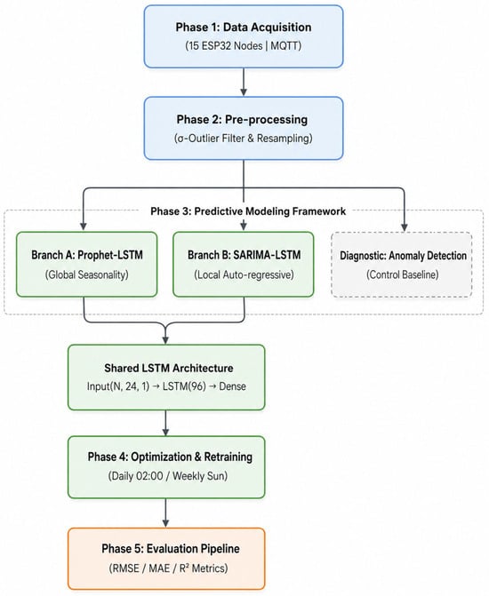
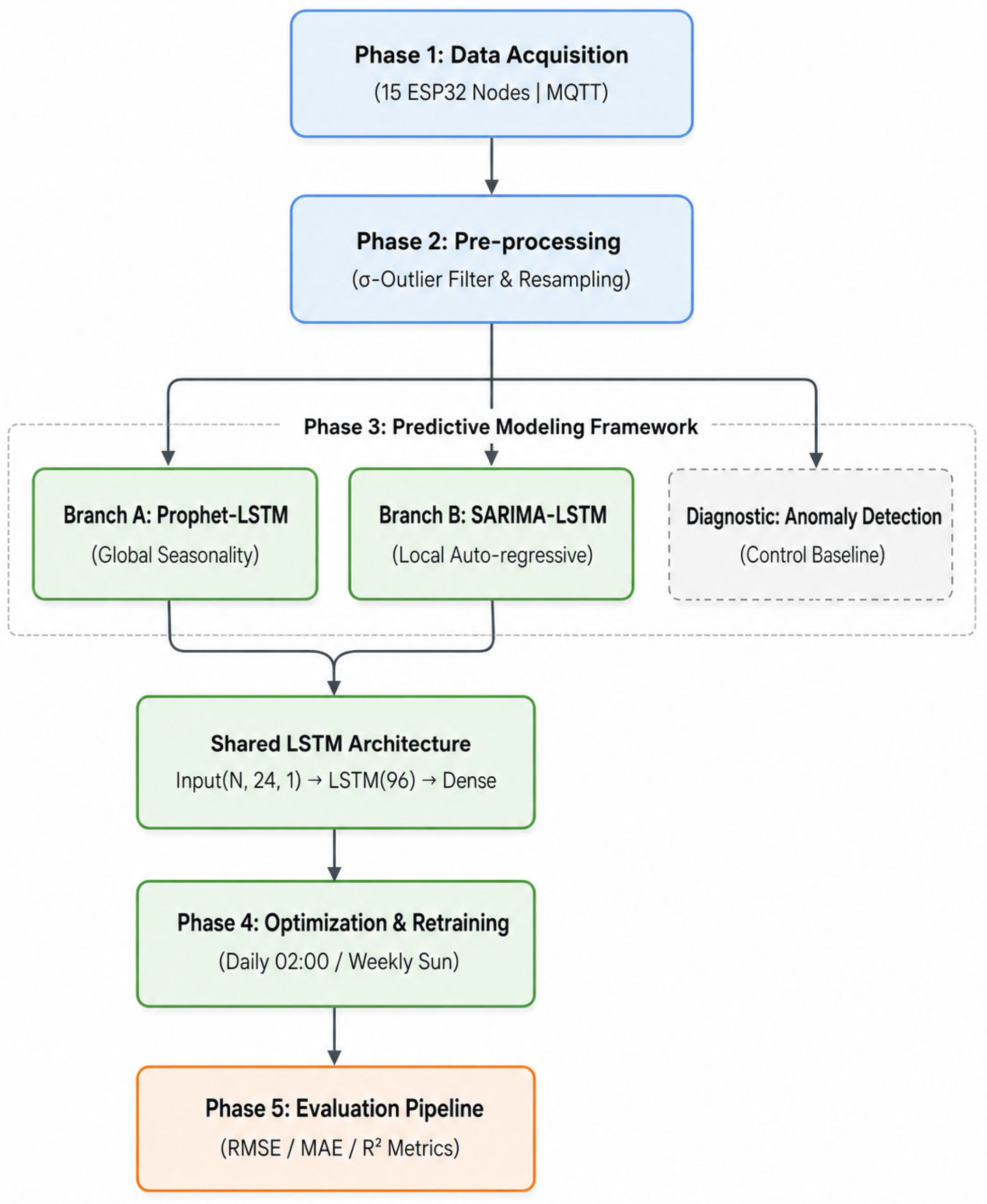
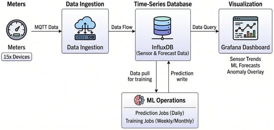
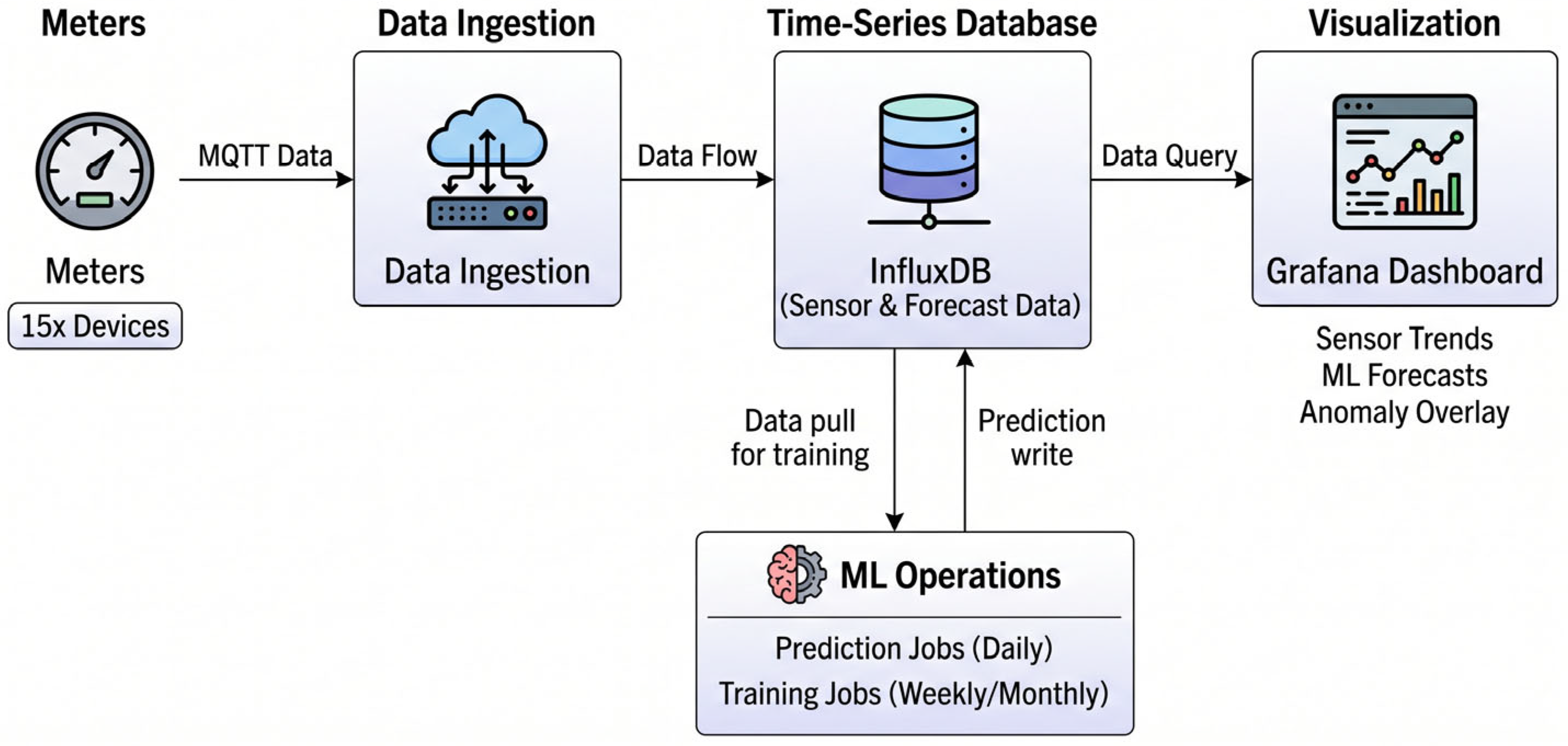
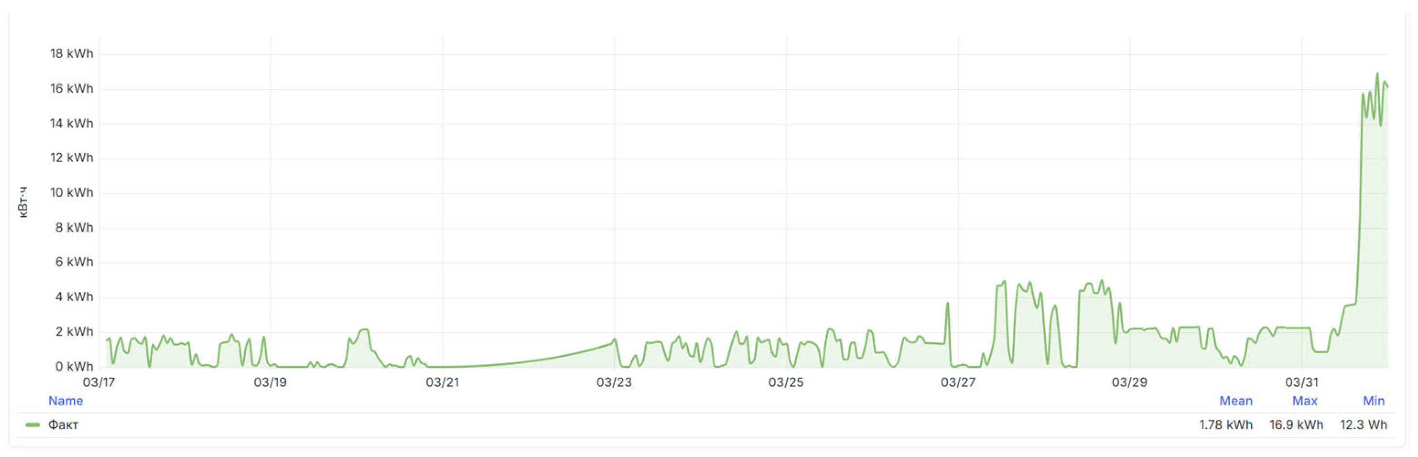
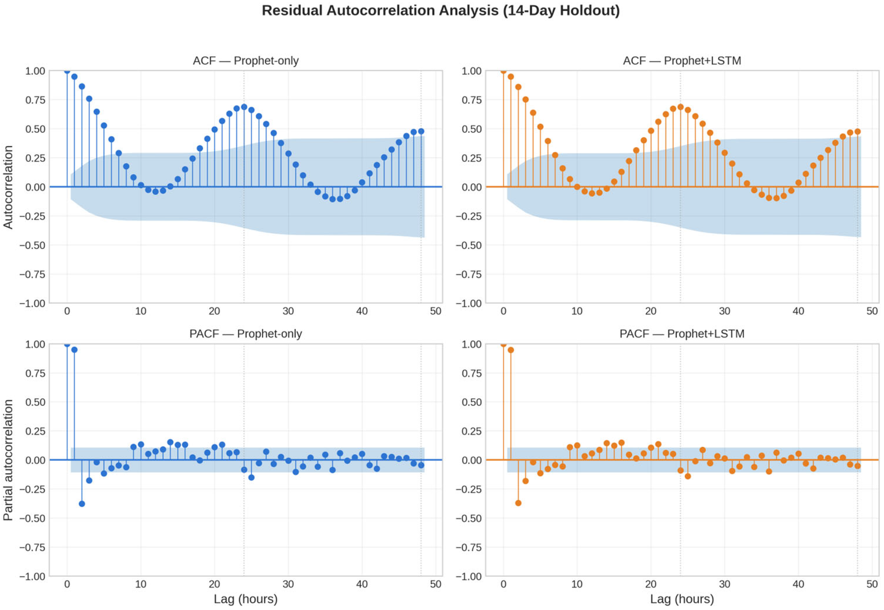
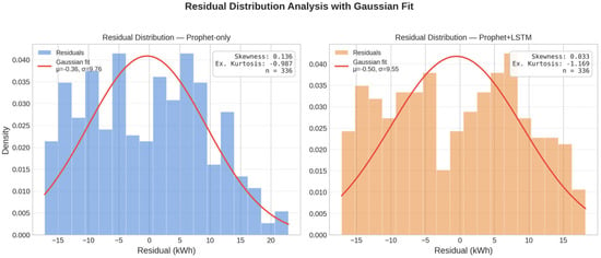
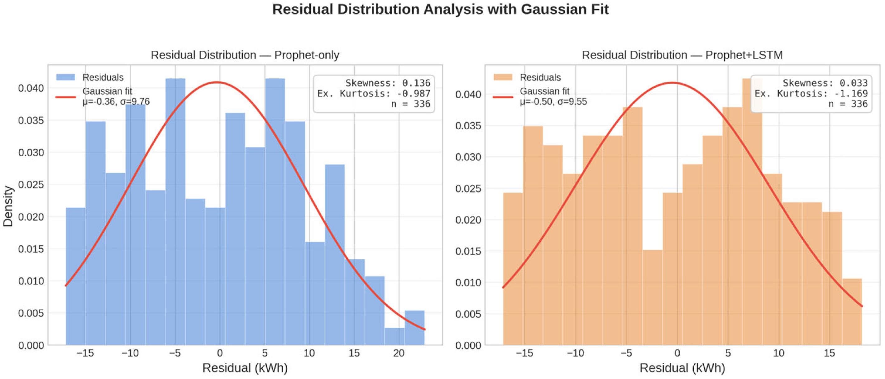

Disclaimer/Publisher’s Note: The statements, opinions and data contained in all publications are solely those of the individual author(s) and contributor(s) and not of MDPI and/or the editor(s). MDPI and/or the editor(s) disclaim responsibility for any injury to people or property resulting from any ideas, methods, instructions or products referred to in the content. |
© 2026 by the authors. Licensee MDPI, Basel, Switzerland. This article is an open access article distributed under the terms and conditions of the Creative Commons Attribution (CC BY) license.