Exact Solutions and Periodic Dynamics of a Three-Dimensional Nonlinear Difference System with Delayed Cyclic Interactions

Abstract

This paper investigates a nonlinear three-dimensional system of difference equations describing the interaction among three mutually dependent sequences evolving over discrete time. The proposed model accounts for nonlinear coupling effects as well as feedback structures that govern the system’s dynamics. We first establish the conditions ensuring the well-definedness and solvability of the system, followed by the construction of closed-form expressions of the solutions under appropriate assumptions on the initial data and parameter settings. To support the theoretical findings, numerical experiments are carried out, accompanied by graphical illustrations that reveal the influence of parameter variations on the qualitative dynamics of the system. As an application, we demonstrate how the proposed three-dimensional nonlinear system can be interpreted in the context of delayed cyclic competition among three interacting populations. This application illustrates the relevance of the developed framework to ecological systems exhibiting nonlinear feedback mechanisms and delayed interactions.

1. Introduction

Difference equations and their systems play a pivotal role in modeling discrete-time phenomena across various scientific fields, including biology, economics, physics, engineering, and time series analysis (see, e.g., [1,2,3,4,5]). They provide a powerful mathematical framework for describing the evolution of dynamical processes whose state at a given time depends on one or more states at previous times. Among these, fractional and nonlinear systems of difference equations have attracted particular interest due to their ability to exhibit a wide spectrum of dynamical behaviors, including stability, boundedness, oscillations, bifurcations, and the emergence of periodic orbits (see, e.g., [6,7,8,9,10,11,12,13,14,15]).

Over the past few decades, many studies have focused on the qualitative analysis of high-order, multidimensional systems. Researchers have developed techniques to transform complex nonlinear systems into simpler, more tractable forms, allowing for the derivation of explicit solutions and the analysis of their stability properties. For example, notable contributions include the work of Althagafi and Ghezal [16] on the system,

$$\begin{array}{cc}\hfill \forall m\ge 0,& A_{m+1}={\displaystyle \frac{1}{-1+B_{m-q}\left(1+A_{m-2q-1}\left(2+B_{m-3q-2}\right)\right)}},\hfill \\ & B_{m+1}={\displaystyle \frac{1}{-1+A_{m-q}\left(1+B_{m-2q-1}\left(2+A_{m-3q-2}\right)\right)}},\hfill \end{array}$$

and Hassani et al. [17] on the system

$$\begin{array}{cc}\hfill \forall m\ge 0,& A_{m+1}=\alpha {\displaystyle \frac{A_{m-1}}{B_m-\mu }}{\left({\displaystyle \frac{A_m-\eta }{B_{m-1}}}\right)}^r{B}_m+\eta ,\hfill \\ & B_{m+1}=\beta {\displaystyle \frac{B_{m-1}}{A_m-\eta }}{\left({\displaystyle \frac{B_m-\mu }{A_{m-1}}}\right)}^r{C}_m+\mu ,\hfill \end{array}$$

In addition, several authors have proposed K-dimensional generalizations of well-known two-dimensional systems, aiming to capture more intricate variable interactions and extend the applicability of results obtained for low-dimensional models. In practice, systems of difference equations are not merely theoretical constructs; they also arise naturally as discrete models obtained through the discretization of continuous-time processes. For example, finite-difference schemes and other numerical methods applied to differential equations often generate discrete dynamical systems that preserve important qualitative features of the underlying continuous models. The study of such systems is essential for understanding the behavior of the numerical approximations themselves, including their stability, periodicity, and long-term dynamics. Moreover, difference equations frequently serve as independent modeling tools for phenomena that are inherently observed or recorded at discrete time intervals, such as seasonal population dynamics, economic cycles, and epidemiological processes. In addition to their role as numerical approximations of continuous-time systems, difference equations are frequently used to model ecological interactions that evolve over discrete generations or observation periods. Of particular interest are cyclic competition systems involving three interacting species, where each species has a competitive advantage over one species while being disadvantaged with respect to another. Such interaction structures arise naturally in ecological communities and have been extensively studied in the literature because they can generate rich dynamical behavior, including coexistence, oscillations, and periodic population cycles [18,19,20]. Delayed responses are also common in ecological systems due to maturation periods, reproductive lags, and environmental adaptation mechanisms [21]. These observations provide a natural setting for the study of nonlinear discrete systems with delayed cyclic interactions.

Motivated by the increasing interest in multidimensional nonlinear discrete systems with delayed interactions and by the need to better understand cyclic feedback mechanisms among three interconnected variables, we introduce the following three-dimensional nonlinear difference system:

$$\begin{array}{cc}\hfill \forall m\ge 0,& A_{m+1}=\alpha {\displaystyle \frac{C_{m-1}}{B_m-\mu }}{\left({\displaystyle \frac{A_m-\eta }{B_{m-1}}}\right)}^r{B}_m+\eta ,\hfill \\ \hfill & B_{m+1}=\beta {\displaystyle \frac{A_{m-1}}{C_m-\rho }}{\left({\displaystyle \frac{B_m-\mu }{C_{m-1}}}\right)}^r{C}_m+\mu ,\hfill \\ \hfill & C_{m+1}=\gamma {\displaystyle \frac{B_{m-1}}{A_m-\eta }}{\left({\displaystyle \frac{C_m-\rho }{A_{m-1}}}\right)}^r{A}_m+\rho ,\hfill \end{array}$$

(1)

where $\alpha >0, \beta >0, \gamma >0, \eta \ge 0, \mu \ge 0, \rho \ge 0,$ $r\in \mathbb{N}$ and the initial conditions are $A_{-1},$$B_{-1},$$C_{-1}$, $A_0,$ $B_0$ and $C_0.$ This system models the evolution of three interconnected sequences, incorporating nonlinear interactions and feedback mechanisms capable of generating complex oscillatory dynamics. Our analysis begins by examining the system’s solvability, deriving explicit solutions under specific initial conditions and parameter values. We then determine conditions for the existence of periodic solutions and support the theoretical findings with numerical simulations that illustrate the influence of parameter variations on the system dynamics, emphasizing how small parameter changes can trigger transitions between steady states, oscillations, and the emergence of more intricate behaviors.

From a modeling perspective, systems of the form (1) arise naturally in situations involving three mutually interacting components whose evolution depends not only on their current states but also on delayed information from previous time periods. Such interactions frequently occur in epidemiological processes, population dynamics, ecological food-chain systems, economic cycles, and other complex discrete-time phenomena. The ratio-dependent terms describe nonlinear interaction effects among the components, while the delayed variables capture memory and lag effects that are commonly observed in real-world systems. Furthermore, the parameters $\eta$, $\mu$, and $\rho$ may be interpreted as baseline levels, threshold values, or external inputs that prevent the complete depletion of the corresponding variables. Consequently, model (1) provides a flexible mathematical framework for investigating cyclic feedback mechanisms, delayed responses, and nonlinear coupling in multivariable discrete dynamical systems. A concrete interpretation of the proposed framework is presented in Section 4, where the variables are associated with the susceptible, infected, and recovered classes of a discrete-time SIR epidemic model. This application illustrates how the mathematical structure of (1) can capture delayed and nonlinear interactions arising in realistic population-based processes.

The main contributions of this paper can be summarized as follows. First, a new class of three-dimensional nonlinear difference equations with delayed ratio-dependent interactions is introduced and analyzed. Second, explicit solution formulas are derived for several important configurations of the system, providing a deeper understanding of its dynamical behavior and solvability. Third, sufficient conditions for the existence of periodic solutions are established, shedding light on the mechanisms underlying recurrent oscillatory dynamics. Fourth, extensive numerical simulations are performed to validate the theoretical results and illustrate the sensitivity of the system to variations in the model parameters. Finally, the applicability of the proposed framework is demonstrated through a discrete-time SIR-type epidemic model, showing how the developed theoretical results can be interpreted and utilized in the study of real-world processes involving delayed nonlinear feedback mechanisms.

The present paper advances the existing literature on nonlinear difference equations in several important directions. Compared with the bidimensional higher-order systems studied in [16,17], the proposed model introduces a genuinely three-dimensional structure with cyclic delayed interactions among all variables, leading to a richer dynamical framework. Unlike many previous studies that focused primarily on stability analysis, asymptotic behavior, or specific solvable cases, the present paper combines the derivation of explicit solution formulas, periodicity analysis, numerical investigations, and application-oriented interpretation within a unified framework. Moreover, while recent studies on three-dimensional systems have established closed-form solutions for particular rational difference equations [22,23,24,25], the system considered here incorporates ratio-dependent nonlinear feedback together with delayed power-type interactions, thereby extending the analytical scope of existing results. The obtained explicit formulas and periodicity criteria provide new insights into the dynamics of multidimensional nonlinear discrete systems and contribute to the ongoing development of analytical techniques for the study of delayed and strongly coupled difference equations.

Despite significant progress in the study of nonlinear difference equations, much of the existing literature focuses on one- and two-dimensional models or on systems with relatively simple interaction structures. In contrast, the system investigated in this paper combines three-dimensional coupling, delayed interactions, ratio-dependent nonlinearity, and nonlinear feedback mechanisms within a unified framework. The novelty of this work lies not only in the introduction of this new class of nonlinear difference equations, but also in the derivation of explicit solution formulas and periodicity criteria that enable a precise characterization of the system’s dynamics. These results contribute to the theoretical development of discrete nonlinear dynamical systems and provide analytical tools for applications involving delayed feedback, nonlinear interactions, and recurrent dynamical behaviors.

2. Solving the System of Equations in (1)

This section focuses on deriving solutions to the system presented in (1), assuming specific initial conditions. Let $\left(A_m,B_m,C_m\right)$ denote a solution sequence defined for all $m\ge -1$. It is important to emphasize that the system becomes ill-defined when certain initial values are set to zero, particularly for indices $\left\{-1, 0\right\}$. Likewise, the formulation breaks down if any of the conditions $A_0=\eta$, $B_0=\mu$ and $C_0=\rho$ hold. To ensure the existence and consistency of a well-defined solution $\left(A_m,B_m,C_m\right)$ across the desired domain, the following conditions must be satisfied for all $m\ge -1$: $A_m{B}_m{C}_m\ne 0$, $A_0\ne \eta ,$ $B_0\ne \mu$ and $C_0\ne \rho$ for $m\ge -1.$ For a strict positivity of the solution, it is additionally required that

$$A_{-1},B_{-1},C_{-1}>0,A_0>\eta ,B_0>\mu \mathrm{and}{C}_0>\rho .$$

(2)

These constraints guarantee that the recursive relations remain well-defined and avoid singularities throughout the iteration process. To simplify the system (1) and to streamline the analysis, we perform a change of variables as follows:

$${\widehat{A}}_m={\displaystyle \frac{A_m-\eta }{B_{m-1}}},{\widehat{B}}_m={\displaystyle \frac{B_m-\mu }{C_{m-1}}},{\widehat{C}}_m={\displaystyle \frac{C_m-\rho }{A_{m-1}}}\mathrm{for}m\ge 0.$$

(3)

This transformation re-expresses the original system in a more tractable form:

$${\widehat{A}}_{m+1}=\alpha {\displaystyle \frac{{\widehat{A}}_m^r}{{\widehat{B}}_m}},\hspace{1em}{\widehat{B}}_{m+1}=\beta {\displaystyle \frac{{\widehat{B}}_m^r}{{\widehat{C}}_m}},\hspace{1em}{\widehat{C}}_{m+1}=\gamma {\displaystyle \frac{{\widehat{C}}_m^r}{{\widehat{A}}_m}}\mathrm{for}m\ge 0.$$

(4)

This reformulated system (4) provides a recursive structure that facilitates the study of the system’s dynamics. Furthermore, we introduce the logarithmic variables: ${\overline{A}}_m,$ ${\overline{B}}_m$ and ${\overline{C}}_m$ the logarithms of ${\widehat{A}}_m,$ ${\widehat{B}}_m$ and ${\widehat{C}}_m$ respectively for $m\ge 0.$ By applying this change of variables, the system in (4) simplifies to a linear system of coupled recurrence relations:

$$\left\{\begin{array}{cc}\hfill {\overline{A}}_{m+1}=& \log \alpha +r{\overline{A}}_m-{\overline{B}}_m,\mathrm{for}m\ge 0\hfill \\ \hfill {\overline{B}}_{m+1}=& \log \beta +r{\overline{B}}_m-{\overline{C}}_m,\hfill \\ \hfill {\overline{C}}_{m+1}=& \log \gamma +r{\overline{C}}_m-{\overline{A}}_m.\hfill \end{array}\right.$$

(5)

Next, we transform system (5) by introducing the variables:

$$\begin{array}{c}{D}_m={\overline{A}}_m+{\overline{B}}_m+{\overline{C}}_m,E_m={\overline{A}}_m-{\overline{B}}_m-{\overline{C}}_m,F_m=-{\overline{A}}_m-{\overline{B}}_m+{\overline{C}}_m\mathrm{for} m\ge 0.\end{array}$$

(6)

Substituting the definitions in (6) into (5), we obtain

$$\left\{\begin{array}{cc}\hfill D_{m+1}=& \log \left(\alpha \beta \gamma \right)+\left(r-1\right)D_m,\mathrm{for}m\ge 0\hfill \\ \hfill E_{m+1}=& \log \left(\alpha /\beta \gamma \right)+r{E}_m+F_m,\hfill \\ \hfill F_{m+1}=& \log \left(\gamma /\alpha \beta \right)+r{F}_m-E_m.\hfill \end{array}\right.$$

(7)

The following theorem provides explicit formulas for the sequences $(D_m,E_m,F_m)$ satisfying the linear system (7). These formulas constitute the key step toward obtaining explicit solutions of the original nonlinear system (1).

Theorem 1.

Let $\left(D_m,E_m,F_m\right)$ be a well-defined solution of the system (7). Then:

i.

If $r\ge 1$, the explicit solution is given by the Formulas (8)–(16).

ii.

If $r=0$, the explicit solution is given by (8) and (17).

Proof. 

Starting from the first equation of (7), we obtain the recurrence:

$$D_m={\displaystyle \sum _{k=0}^{m-1}}{\left(r-1\right)}^k\log \left(\alpha \beta \gamma \right)+{\left(r-1\right)}^m{D}_0,\mathrm{for}m\ge 0.$$

From this, the explicit form for $D_m$ follows as:

$$D_m=\left\{\begin{array}{cc}{\delta }_{2p}\left(m\right)\log \left(\alpha \beta \gamma \right)+{\left(-1\right)}^{m+1}{D}_0\hfill & \mathrm{if}r=0,\\ \log \left(\alpha \beta \gamma \right)\hfill & \mathrm{if}r=1,\\ m\log \left(\alpha \beta \gamma \right)+D_0\hfill & \mathrm{if}r=2,\\ {\displaystyle \frac{{\left(r-1\right)}^m-1}{r-2}}\log \left(\alpha \beta \gamma \right)+{\left(r-1\right)}^m{D}_0\hfill & \mathrm{if}r\ge 3,\end{array}\right.$$

(8)

where ${\delta }_n\left(m\right)$ denotes the Kronecker delta: ${\delta }_n\left(m\right)=\left\{\begin{array}{cc}\hfill 1& \mathrm{if}n=m\\ \hfill 0& \mathrm{if}n\ne m\end{array}\right.$. The remaining two equations in (7) can be expressed in vector form:

$$\begin{array}{cc}\hfill {\underline{G}}_{m+1}:=\left(\begin{array}{c}{E}_{m+1}\\ F_{m+1}\end{array}\right)& =\left(\begin{array}{c}\log \left(\alpha /\beta \gamma \right)\\ \log \left(\gamma /\alpha \beta \right)\end{array}\right)+\left(\begin{array}{cc}r\hfill & 1\\ -1\hfill & r\end{array}\right){\underline{G}}_m,\hfill \\ & :=\underline{\Pi }+\left(r{I}_{\left(2\right)}+J\right){\underline{G}}_m,\hfill \end{array}$$

where $I_{\left(2\right)}$ is the $2\times 2$ identity matrix and $J=\left(\begin{array}{cc}0\hfill & 1\\ -1\hfill & 0\end{array}\right).$ By iterative expansion, we obtain:

$${\underline{G}}_m={\displaystyle {\displaystyle \sum _{k=0}^{m-1}}}{\displaystyle {\displaystyle \sum _{l=0}^k}}{C}_k^l{r}^{k-l}{J}^l\left(\begin{array}{c}\log \left(\alpha /\beta \gamma \right)\\ \log \left(\gamma /\alpha \beta \right)\end{array}\right)+{\displaystyle {\displaystyle \sum _{k=0}^m}}{C}_m^k{r}^{m-k}{J}^k{\underline{G}}_0.$$

This representation allows us to identify the periodic patterns in $E_m$ and $F_m$ with respect to $m\left(\mathrm{mod}4\right)$ and to explicitly separate the contributions from the initial conditions and the constant forcing terms. Careful computation yields the closed-form expressions, covering the cases $m\equiv 0, 1, 2, 3$ $\left(\mathrm{mod}4\right)$. Each case reflects a distinct structure in the binomial expansions and alternating signs arising from the powers of J: for $r\ge 1,$

$$\begin{array}{cc}\hfill E_{4m}=& {\displaystyle \sum _{l=0}^{m-1}}\log \left({\left(\alpha /\beta \gamma \right)}^{L_1\left(r,l,4m-1\right)}{\left(\gamma /\alpha \beta \right)}^{L_2\left(r,l,4m-1\right)}\right)\hfill \\ \hfill & +E_0+{\displaystyle {\displaystyle \sum _{k=0}^{m-1}}}{L}_5\left(r,k,4m\right)E_0+{\displaystyle {\displaystyle \sum _{k=0}^{m-1}}}{L}_4\left(r,k,4m\right)F_0,\hfill \end{array}$$

(9)

$$\begin{array}{cc}\hfill F_{4m}=& {\displaystyle \sum _{l=0}^{m-1}}\log \left({\left(\gamma /\alpha \beta \right)}^{L_1\left(r,l,4m-1\right)}{\left(\alpha /\beta \gamma \right)}^{-L_2\left(r,l,4m-1\right)}\right)\hfill \\ \hfill & +F_0+{\displaystyle \sum _{k=0}^{m-1}}\left(L_3\left(r,k,4m\right)F_0-L_4\left(r,k,4m\right)E_0\right),\hfill \end{array}$$

(10)

$$\begin{array}{cc}\hfill E_{4m+1}=& \log \left(\alpha /\beta \gamma \right)+{\displaystyle \sum _{l=0}^{m-1}}\log \left({\left(\alpha /\beta \gamma \right)}^{L_1\left(r,l,4m\right)}{\left(\gamma /\alpha \beta \right)}^{L_2\left(r,l,4m+1\right)}\right)\hfill \\ \hfill & +\left(\left(4m+1\right)r+{\displaystyle \sum _{k=0}^{m-1}}{L}_5\left(r,k,4m+1\right)\right)E_0+\left(1+{\displaystyle \sum _{k=0}^{m-1}}{L}_4\left(r,k,4m+1\right)\right)F_0,\hfill \end{array}$$

(11)

$$\begin{array}{cc}\hfill F_{4m+1}=& \log \left(\gamma /\alpha \beta \right)+{\displaystyle \sum _{l=0}^{m-1}}\log \left({\left(\gamma /\alpha \beta \right)}^{L_1\left(r,l,4m\right)}{\left(\alpha /\beta \gamma \right)}^{-L_2\left(r,l,4m\right)}\right)\hfill \\ \hfill & +\left(\left(4m+1\right)r+{\displaystyle \sum _{k=0}^{m-1}}{L}_3\left(r,k,4m+1\right)\right)F_0-\left(1+{\displaystyle \sum _{k=0}^{m-1}}{L}_4\left(r,k,4m+1\right)\right)E_0,\hfill \end{array}$$

(12)

$$\begin{array}{cc}\hfill E_{4m+2}=& \left(1+\left(4m+1\right)r\right)\log \left(\alpha /\beta \gamma \right)+{\displaystyle \sum _{l=0}^{m-1}}\log \left({\left(\alpha /\beta \gamma \right)}^{L_1\left(r,l,4m+1\right)}{\left(\gamma /\alpha \beta \right)}^{L_2\left(r,l,4m+1\right)}\right)\hfill \\ \hfill & +{\displaystyle \sum _{k=0}^m}{L}_5\left(r,k,4m+2\right)E_0+\left(\left(4m+2\right)r+{\displaystyle \sum _{k=0}^{m-1}}{L}_4\left(r,k,4m+2\right)\right)F_0,\hfill \end{array}$$

(13)

$$\begin{array}{cc}\hfill F_{4m+2}=& \left(1+\left(4m+1\right)r\right)\log \left(\gamma /\alpha \beta \right)+{\displaystyle \sum _{l=0}^{m-1}}\log \left({\left(\gamma /\alpha \beta \right)}^{L_1\left(r,l,4m+1\right)}{\left(\alpha /\beta \gamma \right)}^{-L_2\left(r,l,4m+1\right)}\right)\hfill \\ \hfill & +{\displaystyle \sum _{k=0}^m}{L}_3\left(r,k,4m+2\right)F_0-\left(\left(4m+2\right)r+{\displaystyle \sum _{k=0}^{m-1}}{L}_4\left(r,k,4m+2\right)\right)E_0,\hfill \end{array}$$

(14)

$$\begin{array}{cc}\hfill E_{4m+3}=& \log {\left(\gamma /\alpha \beta \right)}^{\left(1+\left(4m+2\right)r\right)}+{\displaystyle {\displaystyle \sum _{l=0}^{m-1}}}\log {\left(\gamma /\alpha \beta \right)}^{L_2\left(r,l,4m+2\right)}+{\displaystyle {\displaystyle \sum _{l=0}^m}}\log {\left(\alpha /\beta \gamma \right)}^{L_1\left(r,l,4m+2\right)}\hfill \\ \hfill & +{\displaystyle \sum _{k=0}^m}\left(L_5\left(r,k,4m+3\right)E_0+L_4\left(r,k,4m+3\right)F_0\right),\hfill \end{array}$$

(15)

$$\begin{array}{cc}\hfill F_{4m+3}=& \log {\left(\alpha /\beta \gamma \right)}^{-\left(1+\left(4m+2\right)r\right)}+{\displaystyle {\displaystyle \sum _{l=0}^{m-1}}}\log {\left(\alpha /\beta \gamma \right)}^{-L_2\left(r,l,4m+2\right)}+{\displaystyle {\displaystyle \sum _{l=0}^m}}\log {\left(\gamma /\alpha \beta \right)}^{L_1\left(r,l,4m+2\right)}\hfill \\ \hfill & +{\displaystyle \sum _{k=0}^m}\left(L_3\left(r,k,4m+3\right)F_0-L_4\left(r,k,4m+3\right)E_0\right),\hfill \end{array}$$

(16)

where

$$\begin{array}{c}{L}_1\left(r,l,m\right)={\displaystyle {\displaystyle \sum _{k=4l}^m}}{C}_k^{4l}{r}^{k-4l}-{\displaystyle {\displaystyle \sum _{k=4l+2}^m}}{C}_k^{4l+2}{r}^{k-4l-2},\hfill \\ L_2\left(r,l,m\right)={\displaystyle {\displaystyle \sum _{k=4l+1}^m}}{C}_k^{4l+1}{r}^{k-4l-1}-{\displaystyle {\displaystyle \sum _{k=4l+3}^m}}{C}_k^{4l+3}{r}^{k-4l-3},\hfill \\ L_3\left(r,k,m\right)=C_m^{4k}{r}^{m-4k}+C_m^{4k+2}{r}^{m-4k-2},\hfill \\ L_4\left(r,k,m\right)=C_m^{4k+1}{r}^{m-4k-1}-C_m^{4k+3}{r}^{m-4k-3},\hfill \\ L_5\left(r,k,m\right)=C_m^{4k}{r}^{m-4k}-C_m^{4k+2}{r}^{m-4k-2}.\hfill \end{array}$$

When $r=0$, the last two equations of the system (7) reduce to:

$$\left\{\begin{array}{cc}\hfill E_{m+1}=& -\log \left({\beta }^2\right)-E_{m-1},\hfill \\ \hfill F_{m+1}=& \log \left({\gamma }^2/{\alpha }^2\right)-F_{m-1}.\hfill \end{array}\right.$$

Solving this recurrence yields the periodic solutions $\left(E_m,F_m\right)$, showing a fixed pattern over four consecutive terms:

$$\left(E_m\right):\left\{\begin{array}{c}{E}_{4m}=E_0\hfill \\ E_{4m+1}=-\log \left({\beta }^2\right)-E_{-1}\hfill \\ E_{4m+2}=-\log \left({\beta }^2\right)-E_0\hfill \\ E_{4m+3}=E_{-1}\hfill \end{array}\right.,\left(F_m\right):\left\{\begin{array}{c}{F}_{4m}=F_0\hfill \\ F_{4m+1}=\log \left({\gamma }^2/{\alpha }^2\right)-F_{-1}\hfill \\ F_{4m+2}=\log \left({\gamma }^2/{\alpha }^2\right)-F_0\hfill \\ F_{4m+3}=F_{-1}.\hfill \end{array}\right.$$

(17)

This concludes the proof. □

The derivation of explicit solutions for dynamical systems plays a central role in revealing the internal structure of complex mathematical models. In the context of the transformed system (5), obtaining accurate analytical representations of the solutions under the well-definedness conditions is crucial, as it enables precise control over the behavior of the sequences $\left({\overline{A}}_m, {\overline{B}}_m, {\overline{C}}_m\right)$ across various initial parameter values. Building upon the earlier results concerning variable transformations and the resulting recurrence relations, we can characterize the solution forms according to the value of the parameter r, distinguishing between the cases $r\ge 1$ and $r=0$. This leads naturally to a bifurcated analysis in which each scenario is examined separately. The following corollary summarizes these explicit solutions in a unified form, providing a foundation for further theoretical exploration of the system.

Corollary 1.

Let $\left({\overline{A}}_m,{\overline{B}}_m,{\overline{C}}_m\right)$ be a well-defined solution of the system (5). Then:

i.

If $r\ge 1$, the solutions exhibit 4-periodic patterns in the index m, and are expressed as follows:

$$\left({\overline{A}}_m\right):\left\{\begin{array}{cc}2{\overline{A}}_{4m}\hfill & =E_0+{\delta }_1\left(r\right)\log \left(\alpha \beta \gamma \right)+\left(\log {\left(\alpha \beta \gamma \right)}^{4m}+D_0\right){\delta }_2\left(r\right)\hfill \\ \hfill & +\left({\displaystyle \frac{{\left(r-1\right)}^{4m}-1}{r-2}}\log \left(\alpha \beta \gamma \right)+{\left(r-1\right)}^{4m}{D}_0\right){\displaystyle \sum _{l\ge 3}}{\delta }_l\left(r\right)\hfill \\ \hfill & +{\displaystyle \sum _{k=0}^{m-1}}\log \left({\left(\alpha /\beta \gamma \right)}^{L_1\left(r,k,4m-1\right)}{\left(\gamma /\alpha \beta \right)}^{L_2\left(r,k,4m-1\right)}\right)\hfill \\ \hfill & +{\displaystyle \sum _{k=0}^{m-1}}\left(L_5\left(r,k,4m\right)E_0+L_4\left(r,k,4m\right)F_0\right),\hfill \\ 2{\overline{A}}_{4m+1}\hfill & =\log \left(\alpha /\beta \gamma \right)+\left(4m+1\right)r{E}_0+{\delta }_1\left(r\right)\log \left(\alpha \beta \gamma \right)+\left(\log {\left(\alpha \beta \gamma \right)}^{4m+1}+1+D_0\right){\delta }_2\left(r\right)\hfill \\ \hfill & +F_0+\left({\displaystyle \frac{{\left(r-1\right)}^{4m+1}-1}{r-2}}\log \left(\alpha \beta \gamma \right)+{\left(r-1\right)}^{4m+1}{D}_0\right){\displaystyle \sum _{l\ge 3}}{\delta }_l\left(r\right)\hfill \\ \hfill & +{\displaystyle \sum _{k=0}^{m-1}}\log \left({\left(\alpha /\beta \gamma \right)}^{L_1\left(r,k,4m\right)}{\left(\gamma /\alpha \beta \right)}^{L_2\left(r,k,4m+1\right)}\right)\hfill \\ \hfill & +{\displaystyle \sum _{k=0}^{m-1}}\left(L_5\left(r,k,4m+1\right)E_0+L_4\left(r,k,4m+1\right)F_0\right),\hfill \\ 2{\overline{A}}_{4m+2}\hfill & ={\delta }_1\left(r\right)\log \left(\alpha \beta \gamma \right)+\left(\log {\left(\alpha \beta \gamma \right)}^{4m+2}+D_0\right){\delta }_2\left(r\right)\hfill \\ \hfill & +\left({\displaystyle \frac{{\left(r-1\right)}^{4m+2}-1}{r-2}}\log \left(\alpha \beta \gamma \right)+{\left(r-1\right)}^{4m+2}{D}_0\right){\displaystyle \sum _{l\ge 3}}{\delta }_l\left(r\right)\hfill \\ \hfill & +\left(1+\left(4m+1\right)r\right)\log \left(\alpha /\beta \gamma \right)+\left(4m+2\right)r{F}_0+{\displaystyle \sum _{k=0}^m}{L}_5\left(r,k,4m+2\right)E_0\hfill \\ \hfill & +{\displaystyle \sum _{l=0}^{m-1}}\left(\log \left({\left(\alpha /\beta \gamma \right)}^{L_1\left(r,l,4m+1\right)}{\left(\gamma /\alpha \beta \right)}^{L_2\left(r,l,4m+1\right)}\right)+L_4\left(r,l,4m+2\right)F_0\right),\hfill \\ 2{\overline{A}}_{4m+3}\hfill & ={\delta }_1\left(r\right)\log \left(\alpha \beta \gamma \right)+\left({\displaystyle \frac{{\left(r-1\right)}^{4m+3}-1}{r-2}}\log \left(\alpha \beta \gamma \right)+{\left(r-1\right)}^{4m+3}{D}_0\right){\displaystyle \sum _{l\ge 3}}{\delta }_l\left(r\right)\hfill \\ \hfill & +\left(\log {\left(\alpha \beta \gamma \right)}^{4m+3}+D_0\right){\delta }_2\left(r\right)+\log {\left(\gamma /\alpha \beta \right)}^{\left(1+\left(4m+2\right)r\right)}+{\displaystyle \sum _{l=0}^{m-1}}\log {\left(\gamma /\alpha \beta \right)}^{L_2\left(r,l,4m+2\right)}\hfill \\ \hfill & +{\displaystyle \sum _{k=0}^m}\left(\log {\left(\alpha /\beta \gamma \right)}^{L_1\left(r,k,4m+2\right)}+L_5\left(r,k,4m+3\right)E_0+L_4\left(r,k,4m+3\right)F_0\right),\hfill \end{array}\right.$$

(18)

$$\left({\overline{B}}_m\right):\left\{\begin{array}{cc}-2{\overline{B}}_{4m}\hfill & =F_0+{\displaystyle \sum _{l=0}^{m-1}}\log \left({\left(\alpha /\beta \gamma \right)}^{L_1\left(r,l,4m-1\right)-L_2\left(r,l,4m-1\right)}{\left(\gamma /\alpha \beta \right)}^{L_2\left(r,l,4m-1\right)+L_1\left(r,l,4m-1\right)}\right)\hfill \\ \hfill & +E_0+{\displaystyle \sum _{k=0}^{m-1}}\left(\left(L_5\left(r,k,4m\right)-L_4\left(r,k,4m\right)\right)E_0+\left(L_4\left(r,k,4m\right)+L_3\left(r,k,4m\right)\right)F_0\right),\hfill \\ -2{\overline{B}}_{4m+1}\hfill & =-\log \left({\beta }^2\right)+\left(4m+1\right)r\left(E_0+F_0\right)+F_0-E_0\hfill \\ \hfill & +{\displaystyle \sum _{l=0}^{m-1}}\log \left({\left(\alpha /\beta \gamma \right)}^{L_1\left(r,l,4m\right)-L_2\left(r,l,4m\right)}{\left(\gamma /\alpha \beta \right)}^{L_2\left(r,l,4m+1\right)+L_1\left(r,l,4m\right)}\right)\hfill \\ \hfill & +{\displaystyle \sum _{k=0}^{m-1}}\left(L_5\left(r,k,4m+1\right)-L_4\left(r,k,4m+1\right)\right)E_0\hfill \\ \hfill & +{\displaystyle \sum _{k=0}^{m-1}}\left(L_4\left(r,k,4m+1\right)+L_3\left(r,k,4m+1\right)\right)F_0,\hfill \\ -2{\overline{B}}_{4m+2}\hfill & =-\left(1+\left(4m+1\right)r\right)\log \left({\beta }^2\right)\hfill \\ \hfill & +{\displaystyle \sum _{l=0}^{m-1}}\log \left({\left(\alpha /\beta \gamma \right)}^{L_1\left(r,l,4m+1\right)-L_2\left(r,l,4m+1\right)}{\left(\gamma /\alpha \beta \right)}^{L_2\left(r,l,4m+1\right)+L_1\left(r,l,4m+1\right)}\right)\hfill \\ \hfill & +{\displaystyle \sum _{k=0}^m}\left(L_5\left(r,k,4m+2\right)E_0+L_3\left(r,k,4m+2\right)F_0\right)\hfill \\ \hfill & +\left(\left(4m+2\right)r+{\displaystyle \sum _{k=0}^{m-1}}{L}_4\left(r,k,4m+2\right)\right)\left(F_0-E_0\right),\hfill \\ -2{\overline{B}}_{4m+3}\hfill & =\log {\left(\gamma /\alpha \right)}^{2\left(1+\left(4m+2\right)r\right)}+{\displaystyle {\displaystyle \sum _{l=0}^{m-1}}}\log {\left(\gamma /\alpha \beta \right)}^{2L_2\left(r,l,4m+2\right)}-{\displaystyle {\displaystyle \sum _{l=0}^m}}\log {\left(\beta \right)}^{2L_1\left(r,l,4m+2\right)}\hfill \\ \hfill & +{\displaystyle \sum _{k=0}^m}\left(L_5\left(r,k,4m+3\right)-L_4\left(r,k,4m+3\right)\right)E_0\hfill \\ \hfill & +{\displaystyle \sum _{k=0}^m}\left(L_4\left(r,k,4m+3\right)+L_3\left(r,k,4m+3\right)\right)F_0,\hfill \end{array}\right.$$

(19)

$$\left({\overline{C}}_m\right):\left\{\begin{array}{cc}2{\overline{C}}_{4m}\hfill & ={\delta }_1\left(r\right)\log \left(\alpha \beta \gamma \right)+\left(\log {\left(\alpha \beta \gamma \right)}^{4m}+D_0\right){\delta }_2\left(r\right)\hfill \\ \hfill & +\left({\displaystyle \frac{{\left(r-1\right)}^{4m}-1}{r-2}}\log \left(\alpha \beta \gamma \right)+{\left(r-1\right)}^{4m}{D}_0\right){\displaystyle \sum _{l\ge 3}}{\delta }_l\left(r\right)\hfill \\ \hfill & +F_0+{\displaystyle \sum _{k=0}^{m-1}}\log \left({\left(\gamma /\alpha \beta \right)}^{L_1\left(r,k,4m-1\right)}{\left(\alpha /\beta \gamma \right)}^{-L_2\left(r,k,4m-1\right)}\right)\hfill \\ \hfill & +{\displaystyle \sum _{k=0}^{m-1}}\left(L_3\left(r,k,4m\right)F_0-L_4\left(r,k,4m\right)E_0\right),\hfill \\ 2{\overline{C}}_{4m+1}\hfill & ={\delta }_1\left(r\right)\log \left(\alpha \beta \gamma \right)+\left(\log {\left(\alpha \beta \gamma \right)}^{4m+1}+1+D_0\right){\delta }_2\left(r\right)\hfill \\ \hfill & +\log \left(\gamma /\alpha \beta \right)+\left(4m+1\right)r{F}_0-E_0\hfill \\ \hfill & +\left({\displaystyle \frac{{\left(r-1\right)}^{4m+1}-1}{r-2}}\log \left(\alpha \beta \gamma \right)+{\left(r-1\right)}^{4m+1}{D}_0\right){\displaystyle \sum _{l\ge 3}}{\delta }_l\left(r\right)\hfill \\ \hfill & +{\displaystyle \sum _{k=0}^{m-1}}\log \left({\left(\gamma /\alpha \beta \right)}^{L_1\left(r,k,4m\right)}{\left(\alpha /\beta \gamma \right)}^{-L_2\left(r,k,4m\right)}\right)\hfill \\ \hfill & +{\displaystyle \sum _{k=0}^{m-1}}\left(L_3\left(r,k,4m+1\right)F_0-L_4\left(r,k,4m+1\right)E_0\right),\hfill \\ 2{\overline{C}}_{4m+2}\hfill & =\left(1+\left(4m+1\right)r\right)\log \left(\gamma /\alpha \beta \right)+{\delta }_1\left(r\right)\log \left(\alpha \beta \gamma \right)+\left(\log {\left(\alpha \beta \gamma \right)}^{4m+2}+D_0\right){\delta }_2\left(r\right)\hfill \\ \hfill & +\left({\displaystyle \frac{{\left(r-1\right)}^{4m+2}-1}{r-2}}\log \left(\alpha \beta \gamma \right)+{\left(r-1\right)}^{4m+2}{D}_0\right){\displaystyle \sum _{l\ge 3}}{\delta }_l\left(r\right)\hfill \\ \hfill & -\left(4m+2\right)r{E}_0+{\displaystyle \sum _{k=0}^m}{L}_3\left(r,k,4m+2\right)F_0\hfill \\ \hfill & +{\displaystyle \sum _{l=0}^{m-1}}\left(\log \left({\left(\gamma /\alpha \beta \right)}^{L_1\left(r,l,4m+1\right)}{\left(\alpha /\beta \gamma \right)}^{-L_2\left(r,l,4m+1\right)}\right)-L_4\left(r,l,4m+2\right)E_0\right),\hfill \\ 2{\overline{C}}_{4m+3}\hfill & =\log {\left(\alpha /\beta \gamma \right)}^{-\left(1+\left(4m+2\right)r\right)}+{\delta }_1\left(r\right)\log \left(\alpha \beta \gamma \right)+\left(\log {\left(\alpha \beta \gamma \right)}^{4m+3}+D_0\right){\delta }_2\left(r\right)\hfill \\ \hfill & +{\displaystyle {\displaystyle \sum _{l=0}^{m-1}}}\log {\left(\alpha /\beta \gamma \right)}^{-L_2\left(r,l,4m+2\right)}+\left({\displaystyle \frac{{\left(r-1\right)}^{4m+3}-1}{r-2}}\log \left(\alpha \beta \gamma \right)+{\left(r-1\right)}^{4m+3}{D}_0\right){\displaystyle \sum _{l\ge 3}}{\delta }_l\left(r\right)\hfill \\ \hfill & +{\displaystyle \sum _{k=0}^m}\left(\log {\left(\gamma /\alpha \beta \right)}^{L_1\left(r,k,4m+2\right)}+L_3\left(r,k,4m+3\right)F_0-L_4\left(r,k,4m+3\right)E_0\right).\hfill \end{array}\right.$$

(20)

ii.

If $r=0$, the solution simplifies significantly, reducing to direct expressions in terms of the initial conditions ${\overline{A}}_0,$ ${\overline{A}}_{-1},$ ${\overline{B}}_0,$ ${\overline{B}}_{-1},$ ${\overline{C}}_0,$ and ${\overline{C}}_{-1}$, combined with logarithmic factors involving α, β, and γ. In this case, the intricate 4-periodic recurrence collapses into linear dependence on the initial data:

$$\left({\overline{A}}_m\right):\left\{\begin{array}{c}2{\overline{A}}_{4m}=\log \left(\alpha \beta \gamma \right)-2{\overline{B}}_0-2{\overline{C}}_0,\hfill \\ 2{\overline{A}}_{4m+1}=-\log \left({\beta }^2\right)+{\overline{A}}_0-{\overline{A}}_{-1}+{\overline{B}}_0+{\overline{B}}_{-1}+{\overline{C}}_0+{\overline{C}}_{-1},\hfill \\ 2{\overline{A}}_{4m+2}=\log \left(\alpha \gamma /\beta \right)-2{\overline{A}}_0,\hfill \\ 2{\overline{A}}_{4m+3}={\overline{A}}_0+{\overline{A}}_{-1}+{\overline{B}}_0-{\overline{B}}_{-1}+{\overline{C}}_0-{\overline{C}}_{-1},\hfill \end{array}\right.$$

(21)

$$\left({\overline{B}}_m\right):\left\{\begin{array}{c}{\overline{B}}_{4m}={\overline{B}}_0,\hfill \\ -2{\overline{B}}_{4m+1}=\log \left({\gamma }^2/{\alpha }^2{\beta }^2\right)+2{\overline{B}}_{-1},\hfill \\ -2{\overline{B}}_{4m+2}=\log \left({\gamma }^2/{\alpha }^2{\beta }^2\right)+2{\overline{B}}_0,\hfill \\ {\overline{B}}_{4m+3}={\overline{B}}_{-1},\hfill \end{array}\right.$$

(22)

$$\left({\overline{C}}_m\right):\left\{\begin{array}{c}2{\overline{C}}_{4m}=\log \left(\alpha \beta \gamma \right)-{\overline{A}}_0-{\overline{B}}_0-{\overline{C}}_0-{\overline{A}}_0-{\overline{B}}_0+{\overline{C}}_0,\hfill \\ 2{\overline{C}}_{4m+1}=\log \left({\gamma }^2/{\alpha }^2\right)+{\overline{A}}_0+{\overline{B}}_0+{\overline{C}}_0+{\overline{A}}_{-1}+{\overline{B}}_{-1}-{\overline{C}}_{-1},\hfill \\ 2{\overline{C}}_{4m+2}=\log \left(\beta {\gamma }^3/\alpha \right)-2{\overline{C}}_0,\hfill \\ 2{\overline{C}}_{4m+3}={\overline{A}}_0+{\overline{B}}_0+{\overline{C}}_0-{\overline{A}}_{-1}-{\overline{B}}_{-1}+{\overline{C}}_{-1}.\hfill \end{array}\right.$$

(23)

Proof. 

The proof begins by applying the inverse variable transformation described in (6), which maps the transformed system back to the original one while preserving the recurrence relationships among the variables. This yields the identities:

$${\overline{A}}_m={\displaystyle \frac{1}{2}}\left(D_m+E_m\right),{\overline{B}}_m={\displaystyle \frac{-1}{2}}\left(E_m+F_m\right),{\overline{C}}_m={\displaystyle \frac{1}{2}}\left(D_m+F_m\right),\mathrm{for}m\ge 0.$$

The relations for ${\overline{A}}_m$, ${\overline{B}}_m$, ${\overline{C}}_m$ are subsequently examined under distinct cases determined by the parameter r:

i.

When $r\ge 1$: In this case, the explicit solution emerges through a structured substitution process, where the initial conditions are embedded into the solution framework via the auxiliary functions $L_i$ $(i=1,\dots ,5)$, ultimately producing the 4-periodic closed-form expressions stated in the corollary. Moreover, the validity of these explicit representations can be verified directly by substitution into the transformed recurrence system. Indeed, the sequences $\left(D_m\right)$, $\left(E_m\right)$, and $\left(F_m\right)$ obtained in the preceding theorem satisfy the corresponding recurrence relations for all admissible indices (m), while the auxiliary functions $\left(L_i\right)$$\left(\right(i=1,\dots ,5\left)\right)$ account for the iterative contributions generated at each stage of the recurrence process. Consequently, substituting the explicit expressions for $\left(D_m\right)$, $\left(E_m\right)$, and $\left(F_m\right)$ into the inverse transformation (6) yields Formulas (18)–(20). These expressions inherit the recurrence structure of the transformed system and satisfy the prescribed initial conditions, thereby confirming the validity of the obtained solutions.

ii.

When $r=0$: This allows for an immediate derivation of the solution, yielding the simplified closed-form formulas. Furthermore, evaluating the obtained formulas at the initial indices recovers precisely the prescribed initial conditions, thereby providing an additional consistency check for the derived closed-form solutions. Therefore, the formulas presented in the corollary constitute valid explicit solutions of system (5). This completes the proof.

□

The recurrence relations governing $\left({\widehat{A}}_m,{\widehat{B}}_m,{\widehat{C}}_m\right)$ display distinct structural behaviors depending on the parameter r. By separating the analysis into specific parameter regimes, we can obtain explicit closed-form expressions that fully characterize the system’s dynamics. The following corollary summarizes these findings.

Corollary 2.

Let $\left({\widehat{A}}_m,{\widehat{B}}_m,{\widehat{C}}_m\right)$ be a well-defined solution of the system (4). Then:

i.

If $r\ge 1$, the solutions exhibit 4-periodic patterns in the index m. Their explicit closed-form expressions are given in (18)–(20).

ii.

If $r=0$, the system reduces to a simpler form, and the sequences $\left({\widehat{A}}_m\right)$, $\left({\widehat{B}}_m\right)$, $\left({\widehat{C}}_m\right)$ are determined by the exponential expressions in (21)–(23).

The following theorem provides an explicit representation of the solutions $\left(A_m, B_m, C_m\right)$ of the nonlinear coupled system (1). This result is of central importance because it reduces the original nonlinear recurrence system into a set of structured closed-form formulas governed by a third-order linear non-homogeneous difference equation with variable coefficients. Such explicit solutions are particularly valuable for both theoretical analysis and practical computation, as they bypass iterative calculation and reveal the intrinsic structure of the dynamics.

Theorem 2.

Let $\left(A_m,B_m,C_m\right)$ be a well-defined solution of the system (1) satisfying the condition (2). Then, for all integers $m\ge 0$, the sequences $\left(A_m\right)$, $\left(B_m\right)$, and $\left(C_m\right)$ admit the following explicit representation:

$$\left\{\begin{array}{c}{A}_{3m}=f_m\left({\widehat{A}}_m\left(0\right),{\widehat{B}}_m\left(0\right),{\widehat{C}}_m\left(0\right)\right)A_0+{\displaystyle \sum _{i=0}^{m-1}}{f}_i\left({\widehat{A}}_m\left(0\right),{\widehat{B}}_m\left(0\right),{\widehat{C}}_m\left(0\right)\right)g_{\rho ,\mu ,\eta }\left({\widehat{A}}_m\left(0\right),{\widehat{B}}_m\left(0\right),i\right),\hfill \\ A_{3m+1}=f_m\left({\widehat{A}}_m\left(1\right),{\widehat{B}}_m\left(1\right),{\widehat{C}}_m\left(1\right)\right)A_1+{\displaystyle \sum _{i=0}^{m-1}}{f}_i\left({\widehat{A}}_m\left(1\right),{\widehat{B}}_m\left(1\right),{\widehat{C}}_m\left(1\right)\right)g_{\rho ,\mu ,\eta }\left({\widehat{A}}_m\left(1\right),{\widehat{B}}_m\left(1\right),i\right),\hfill \\ A_{3m+2}=f_{m+1}\left({\widehat{A}}_m\left(2\right),{\widehat{B}}_m\left(2\right),{\widehat{C}}_m\left(2\right)\right)A_{-1}+{\displaystyle \sum _{i=0}^m}{f}_i\left({\widehat{A}}_m\left(2\right),{\widehat{B}}_m\left(2\right),{\widehat{C}}_m\left(2\right)\right)g_{\rho ,\mu ,\eta }\left({\widehat{A}}_m\left(2\right),{\widehat{B}}_m\left(2\right),i\right),\hfill \end{array}\right.$$

$$\left\{\begin{array}{c}{B}_{3m}=f_m\left({\widehat{B}}_m\left(0\right),{\widehat{C}}_m\left(0\right),{\widehat{A}}_m\left(0\right)\right)B_0+{\displaystyle \sum _{i=0}^{m-1}}{f}_i\left({\widehat{B}}_m\left(0\right),{\widehat{C}}_m\left(0\right),{\widehat{A}}_m\left(0\right)\right)g_{\eta ,\rho ,\mu }\left({\widehat{B}}_m\left(0\right),{\widehat{C}}_m\left(0\right),i\right),\hfill \\ B_{3m+1}=f_m\left({\widehat{B}}_m\left(1\right),{\widehat{C}}_m\left(1\right),{\widehat{A}}_m\left(1\right)\right)B_1+{\displaystyle \sum _{i=0}^{m-1}}{f}_i\left({\widehat{B}}_m\left(1\right),{\widehat{C}}_m\left(1\right),{\widehat{A}}_m\left(1\right)\right)g_{\eta ,\rho ,\mu }\left({\widehat{B}}_m\left(1\right),{\widehat{C}}_m\left(1\right),i\right),\hfill \\ B_{3m+2}=f_{m+1}\left({\widehat{B}}_m\left(2\right),{\widehat{C}}_m\left(2\right),{\widehat{A}}_m\left(2\right)\right)B_{-1}+{\displaystyle \sum _{i=0}^m}{f}_i\left({\widehat{B}}_m\left(2\right),{\widehat{C}}_m\left(2\right),{\widehat{A}}_m\left(2\right)\right)g_{\eta ,\rho ,\mu }\left({\widehat{B}}_m\left(2\right),{\widehat{C}}_m\left(2\right),i\right),\hfill \end{array}\right.$$

$$\left\{\begin{array}{c}{C}_{3m}=f_m\left({\widehat{C}}_m\left(0\right),{\widehat{A}}_m\left(0\right),{\widehat{B}}_m\left(0\right)\right)C_0+{\displaystyle \sum _{i=0}^{m-1}}{f}_i\left({\widehat{C}}_m\left(0\right),{\widehat{A}}_m\left(0\right),{\widehat{B}}_m\left(0\right)\right)g_{\mu ,\eta ,\rho }\left({\widehat{C}}_m\left(0\right),{\widehat{A}}_m\left(0\right),i\right),\hfill \\ C_{3m+1}=f_m\left({\widehat{C}}_m\left(1\right),{\widehat{A}}_m\left(1\right),{\widehat{B}}_m\left(1\right)\right)C_1+{\displaystyle \sum _{i=0}^{m-1}}{f}_i\left({\widehat{C}}_m\left(1\right),{\widehat{A}}_m\left(1\right),{\widehat{B}}_m\left(1\right)\right)g_{\mu ,\eta ,\rho }\left({\widehat{C}}_m\left(1\right),{\widehat{A}}_m\left(1\right),i\right),\hfill \\ C_{3m+2}=f_{m+1}\left({\widehat{C}}_m\left(2\right),{\widehat{A}}_m\left(2\right),{\widehat{B}}_m\left(2\right)\right)C_{-1}+{\displaystyle \sum _{i=0}^m}{f}_i\left({\widehat{B}}_m\left(2\right),{\widehat{C}}_m\left(2\right),{\widehat{A}}_m\left(2\right)\right)g_{\mu ,\eta ,\rho }\left({\widehat{C}}_m\left(2\right),{\widehat{A}}_m\left(2\right),i\right),\hfill \end{array}\right.$$

where

$$\begin{array}{cc}{f}_n\left(X_m\left(k\right),Y_m\left(k\right),Z_m\left(k\right)\right)\hfill & ={\displaystyle \prod _{j=0}^{n-1}}{X}_{3\left(m-j\right)+k}{Y}_{3\left(m-j\right)+k-1}{Z}_{3\left(m-j\right)+k-2},n,m,k\ge 0\hfill \\ g_{\rho ,\mu ,\eta }\left(X_m\left(k\right),Y_m\left(k\right),i\right)\hfill & =X_{3\left(m-i\right)+k}{Y}_{3\left(m-i\right)+k-1}\rho +X_{3\left(m-i\right)+k}\mu +\eta ,\hfill \end{array}$$

and the sequences $\left({\widehat{A}}_m\right)$, $\left({\widehat{B}}_m\right)$, and $\left({\widehat{C}}_m\right)$ are determined according to Corollary 2 for both $r\ge 1$ and $r=0$.

Proof. 

We start by applying the inverse change of variables given in (3), which transforms the original system into:

$$\left\{\begin{array}{c}{A}_m={\widehat{A}}_m{B}_{m-1}+\eta ,\mathrm{for}m\ge 0\hfill \\ B_m={\widehat{B}}_m{C}_{m-1}+\mu ,\hfill \\ C_m={\widehat{C}}_m{A}_{m-1}+\rho .\hfill \end{array}\right.$$

By appropriately shifting indices and substituting recursively, we can express each term as a product of three consecutive components plus a non-homogeneous part:

$$\left\{\begin{array}{c}{A}_m={\widehat{A}}_m{\widehat{B}}_{m-1}{\widehat{C}}_{m-2}{A}_{m-3}+{\widehat{A}}_m{\widehat{B}}_{m-1}\rho +{\widehat{A}}_m\mu +\eta ,\hfill \\ B_m={\widehat{B}}_m{\widehat{C}}_{m-1}{\widehat{A}}_{m-2}{B}_{m-3}+{\widehat{B}}_m{\widehat{C}}_{m-1}\eta +{\widehat{B}}_m\rho +\mu ,\hfill \\ C_m={\widehat{C}}_m{\widehat{A}}_{m-1}{\widehat{B}}_{m-2}{C}_{m-3}+{\widehat{C}}_m{\widehat{A}}_{m-1}\mu +{\widehat{C}}_m\eta +\rho .\hfill \end{array}\right.$$

This structure reveals that each component satisfies a linear non-homogeneous third-order difference equation with variable coefficients of the general form:

$$X_m=L_m{X}_{m-3}+K_m.$$

To solve it, we decompose the index m into the three residue classes modulo 3:

$$\left\{\begin{array}{c}{X}_{3m}=L_{3m}{X}_{3\left(m-1\right)}+K_{3m},\hfill \\ X_{3m+1}=L_{3m+1}{X}_{3\left(m-1\right)+1}+K_{3m+1},\hfill \\ X_{3m+2}=L_{3m+2}{X}_{3\left(m-1\right)+2}+K_{3m+2}.\hfill \end{array}\right.$$

Solving each class separately by iteration yields:

$$\left\{\begin{array}{c}{X}_{3m}=\left\{{\displaystyle \prod _{j=0}^{m-1}}{L}_{3\left(m-j\right)}\right\}{X}_0+{\displaystyle \sum _{i=0}^{m-1}}\left\{{\displaystyle \prod _{j=0}^{i-1}}{L}_{3\left(m-j\right)}\right\}{K}_{3\left(m-i\right)},\hfill \\ X_{3m+1}=\left\{{\displaystyle \prod _{j=0}^{m-1}}{L}_{3\left(m-j\right)+1}\right\}{X}_1+{\displaystyle \sum _{i=0}^{m-1}}\left\{{\displaystyle \prod _{j=0}^{i-1}}{L}_{3\left(m-j\right)+1}\right\}{K}_{3\left(m-i\right)+1},\hfill \\ X_{3m+2}=\left\{{\displaystyle \prod _{j=0}^m}{L}_{3\left(m-j\right)+2}\right\}{X}_{-1}+{\displaystyle \sum _{i=0}^m}\left\{{\displaystyle \prod _{j=0}^{i-1}}{L}_{3\left(m-j\right)+2}\right\}{K}_{3\left(m-i\right)+2}.\hfill \end{array}\right.$$

Finally, by substituting $X_m$ with $A_m$, $B_m$, and $C_m$ together with their respective coefficient functions $f_m$ and $g_{\rho ,\mu ,\eta }$, we obtain the stated closed-form solution. □

3. Numerical Examples

In this section, we present several numerical examples to illustrate the theoretical results obtained in the previous section. Each example considers a specific set of parameters and initial conditions, highlighting different dynamical behaviors of the proposed system. The examples are supported by graphical simulations that provide a clearer understanding of the system’s evolution over time.

Example 1.

Consider a system defined by three sequences, $\left(A_m\right)$, $\left(B_m\right)$, and $\left(C_m\right)$, whose evolution is governed by the following set of recursive equations:

$$\begin{array}{ccc}\hfill \forall m\ge 0,& A_{m+1}\hfill & =0.80{\displaystyle \frac{C_{m-1}}{B_m-0.15}}{B}_m+0.10,\hfill \\ \hfill & B_{m+1}\hfill & =0.90{\displaystyle \frac{A_{m-1}}{C_m-0.12}}{C}_m+0.15,\hfill \\ \hfill & C_{m+1}\hfill & =0.95{\displaystyle \frac{B_{m-1}}{A_m-0.10}}{A}_m+0.12.\hfill \end{array}$$

(24)

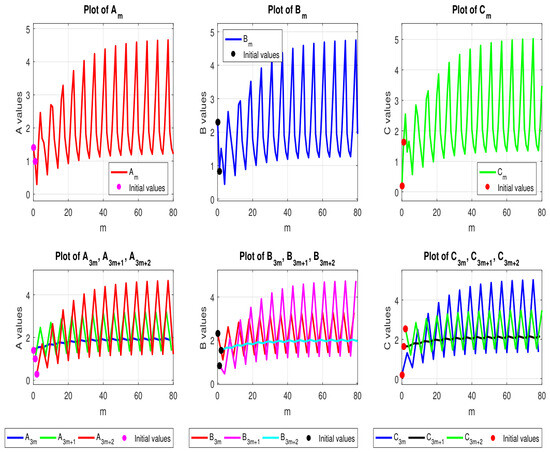
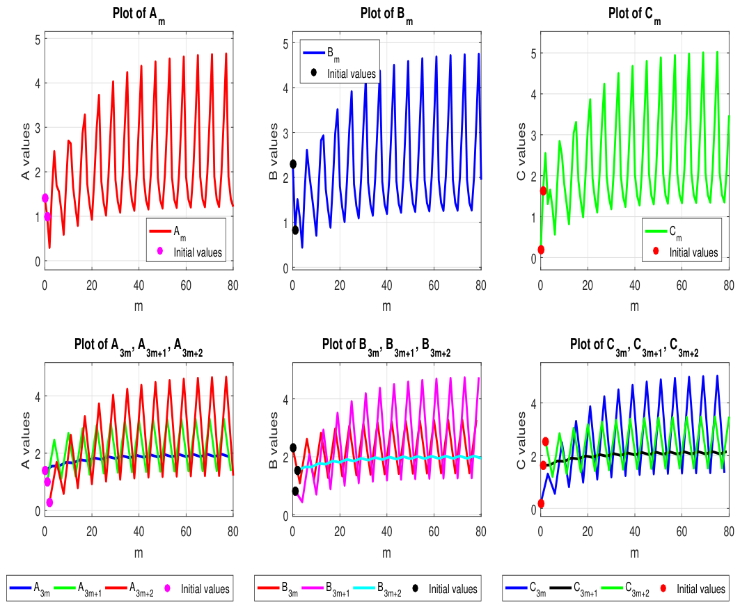
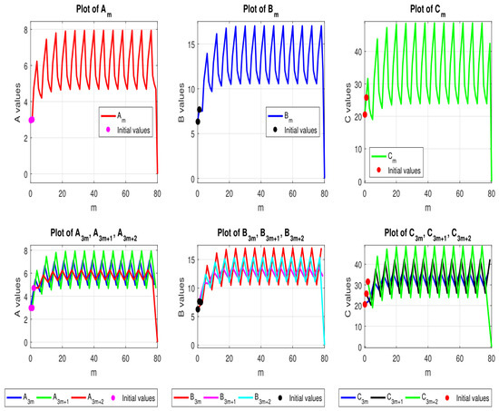
The initial conditions are given by: $A_0=1.0$, $A_{-1}=1.4$, $B_0=0.83$, $B_{-1}=2.3$, $C_0=1.63$, and $C_{-1}=0.2$. To analyze the system, we simulate the sequences $\left(A_m\right)$, $\left(B_m\right)$, and $\left(C_m\right)$ over multiple iterations. The resulting trajectories are plotted in Figure 1, which illustrates the oscillatory patterns and potential convergence properties of the system.

Figure 1. Time evolution of $A_m$, $B_m$, and $C_m$, including the subsequences $3m$, $3m+1$, and $3m+2$ for each variable in the system (24).

Example 2.

We next consider another particular case of the general system (1). In this example, the parameters are chosen as $\alpha =\beta =\gamma =1$, $\eta =0.10$, $\mu =0.15$, $\rho =0.12$, $r=0$. The initial values are $A_0=2.7$, $A_{-1}=2.5$, $B_0=1.65$, $B_{-1}=0.3$, $C_0=2.9$, $C_{-1}=2.3$. Accordingly, system (1) becomes

$$\begin{array}{cccc}\hfill A_{m+1}& ={\displaystyle \frac{C_{m-1}}{B_m-0.15}}{B}_m+0.10,B_{m+1}\hfill & \hfill ={\displaystyle \frac{A_{m-1}}{C_m-0.12}}{C}_m+0.15,C_{m+1}& ={\displaystyle \frac{B_{m-1}}{A_m-0.10}}{A}_m+0.12.\hfill \end{array}$$

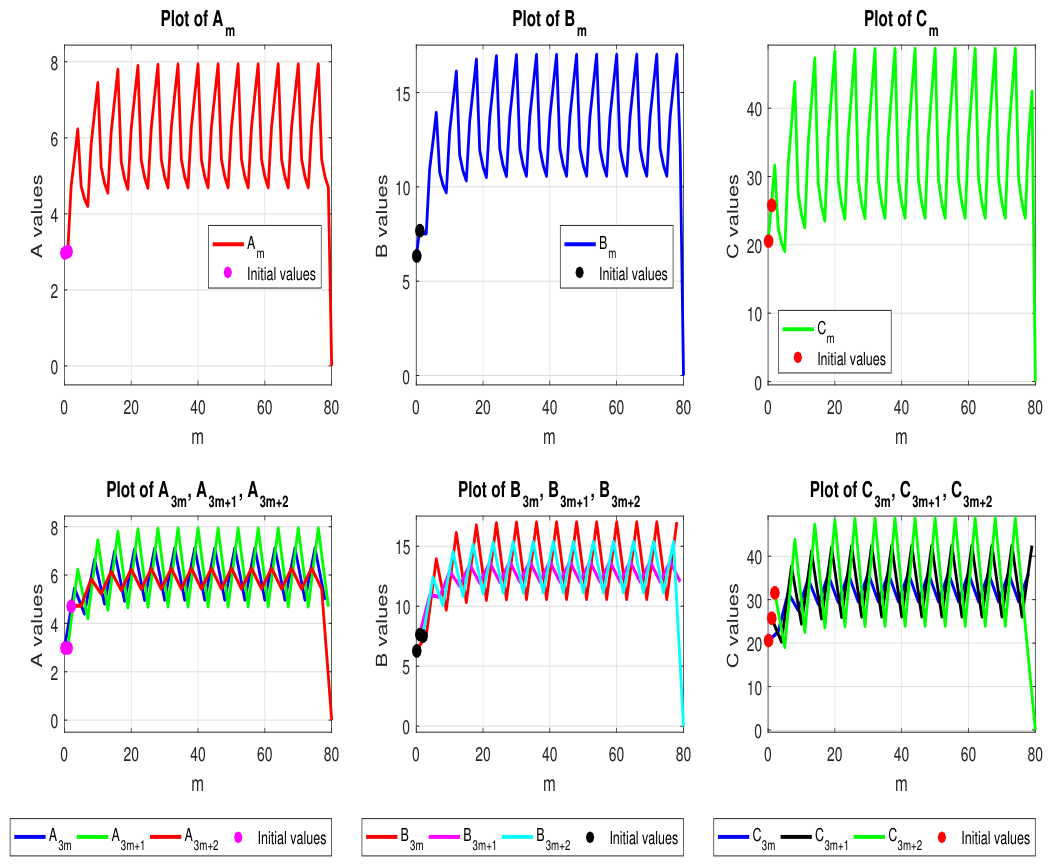
The trajectories of $\left(A_m\right)$, $\left(B_m\right)$, and $\left(C_m\right)$ are displayed in Figure 2.

Figure 2. Time evolution of $A_m$, $B_m$, and $C_m$, including the subsequences $3m$, $3m+1$, and $3m+2$ for each variable in the system (1).

Example 3.

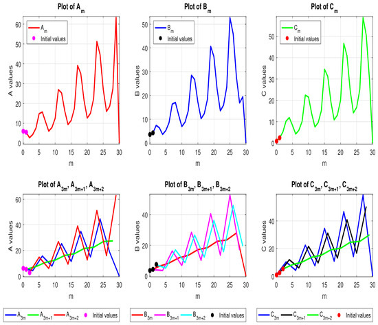
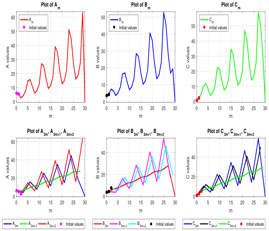
Consider system (1) with $\alpha =0.1, \beta =2, \gamma =1.8$, and $\eta =1.9, \mu =1.6, \rho =1.3$. We choose $r=1$ and the initial conditions $A_{-1}=2, A_0=3, B_{-1}=4, B_0=5, C_{-1}=6, C_0=7$. Figure 3 displays the trajectories of the original variables $\left(A_m\right)$, $\left(B_m\right)$, and $\left(C_m\right)$, together with the corresponding transformed and logarithmic variables. Although the original sequences may attain very large magnitudes, the transformed variables remain well structured. The resulting trajectories are shown in Figure 3.

Figure 3. Dynamical evolution of the sequences $\left(A_m\right)$, $\left(B_m\right)$, and $\left(C_m\right)$ in the critical case $r=1$, together with the corresponding subsequences associated with the residue classes modulo three.

Figure 1 provides a detailed visualization of the dynamical evolution of the sequences $\left(A_m\right)$, $\left(B_m\right)$, and $\left(C_m\right)$ generated by system (24) under the first set of initial conditions. The upper panels show that the three sequences undergo noticeable transient oscillations during the initial iterations before gradually approaching a bounded oscillatory regime. Although the trajectories do not converge to a single equilibrium point, their amplitudes remain confined within relatively narrow intervals throughout the simulation horizon. This behavior indicates that the nonlinear feedback structure of the system prevents divergence while sustaining persistent oscillations. A more informative picture is provided by the lower panels, where the subsequences $\left(A_{3m}\right)$, $\left(A_{3m+1}\right)$, $\left(A_{3m+2}\right)$, $\left(B_{3m}\right)$, $\left(B_{3m+1}\right)$, $\left(B_{3m+2}\right)$, $\left(C_{3m}\right)$, $\left(C_{3m+1}\right)$, and $\left(C_{3m+2}\right)$ are plotted separately. It can be observed that each family of subsequences forms three distinct branches that remain approximately invariant over time. Such a structure provides strong numerical evidence of a period-three oscillatory regime. After the transient stage, the values associated with the same residue class modulo three become nearly repetitive, strongly suggesting the emergence of a stable three-cycle. Moreover, the distances between the corresponding branches remain bounded and nearly constant, indicating that the system approaches a persistent periodic attractor rather than an equilibrium state.

Figure 2 exhibits substantially different behavior from that observed in Figure 1. It should be emphasized, however, that the two examples differ not only in their initial conditions but also in the parameter values of the system. In Example 1, the coefficients are chosen as $\alpha =0.80$, $\beta =0.90$, and $\gamma =0.95$, whereas Example 2 is generated with $\alpha =\beta =\gamma =1$. Therefore, the differences between the two figures cannot be attributed solely to the initial conditions. The trajectories displayed in Figure 2 attain considerably larger amplitudes than those observed in Figure 1. This suggests that the combined effect of the modified parameter values and the new initial conditions leads to a different dynamical regime. In particular, the variables exhibit wider oscillations and larger deviations from their initial states while preserving the same cyclic organization of the dynamics. The lower panels of Figure 2 show that the decomposition into subsequences corresponding to the residue classes $\left(3m\right)$, $(3m+1)$, and $(3m+2)$ still produces three distinct branches, providing numerical evidence for the persistence of a period structure. However, the separation between these branches is significantly larger than that observed in Figure 1, reflecting the stronger oscillatory response associated with the modified parameter configuration and initial conditions.

Consequently, the comparison between Figure 1 and Figure 2 should be interpreted as illustrating the combined influence of changes in both the system parameters and the initial conditions, rather than the effect of varying the initial conditions alone.

Figure 3 illustrates the dynamical behavior of the system in the special case $r=1$, which plays a central role in the theoretical development of the paper. In contrast to the previous examples, the parameter configuration considered here corresponds to the threshold case separating the simplified regime $r=0$ from the more general family of solutions derived for $r\ge 1$. The upper panels show that the sequences $\left(A_m\right)$, $\left(B_m\right),$ and $\left(C_m\right)$ remain positive and bounded throughout the simulation interval while exhibiting persistent oscillatory behavior. Although the amplitudes of the three variables are not identical, their trajectories evolve in a highly organized manner and display no indication of instability or unbounded growth. A more revealing picture is provided by the lower panels, where the sequences are decomposed according to their residue classes modulo three. The resulting plots clearly separate into three recurrent branches for each variable, indicating that values belonging to the same residue class follow nearly identical long-term patterns. This numerical observation is fully consistent with the analytical structure established in the theoretical section, where the explicit solutions are derived by treating the three residue classes separately. Consequently, Figure 3 provides strong numerical evidence that, in the critical case $r=1$, the dynamics preserve the intrinsic period-three organization predicted by the theory. Moreover, the persistence of these distinct branches confirms that the closed-form expressions obtained for $r\ge 1$ accurately capture the periodic mechanism governing the long-term evolution of the system, thereby providing additional support for the analytical results established in Section 2.

Remark 1.

It is worth emphasizing that Example 1 corresponds to the special case $(r=0)$. According to the analytical results established in Section 2, particularly Corollary 2, the transformed variables $\left({\widehat{A}}_m\right)$, $\left({\widehat{B}}_m\right)$, and $\left({\widehat{C}}_m\right)$ admit explicit periodic representations. Consequently, the oscillations observed in Figure 1 should not be interpreted as evidence of instability or chaotic behavior. Rather, they reflect the inherent periodic structure induced by the delayed cyclic coupling of the system. More precisely, the decomposition of the solutions into subsequences corresponding to the residue classes modulo three reveals the emergence of distinct periodic branches. As a result, the trajectories continue to oscillate while remaining uniformly bounded. The observed fluctuations therefore represent a regular periodic alternation among these branches and are fully consistent with the theoretical predictions obtained for the case $(r=0)$. Figure 1 should thus be regarded as a numerical illustration of bounded periodic dynamics rather than irregular or chaotic oscillations.

Remark 2.

It is worth emphasizing that the trajectories displayed in Figure 2 remain strictly positive throughout the entire simulation interval. The apparent disappearance of portions of the curves near $(m=30)$ is merely a graphical effect resulting from the plotting scale and the overlap of oscillatory trajectories. The corresponding solution values remain positive and do not approach zero. Moreover, the subsequent iterates continue to evolve positively while preserving their oscillatory behavior. Therefore, Figure 2 should not be interpreted as indicating extinction or vanishing solutions; rather, it illustrates a positive large-amplitude oscillatory regime that is fully consistent with the theoretical properties of the system.

Remark 3.

The primary purpose of the numerical section is not to provide a comprehensive computational investigation of the system, but rather to illustrate the analytical results established in Section 2. Accordingly, the selected examples were designed to represent the principal parameter regimes covered by the theoretical analysis, namely the special case $r=0$ and the general regime $r\ge 1$. In each example, the numerical trajectories exhibit the same residue-class decomposition predicted by the explicit solution formulas. The observed recurrent oscillatory patterns therefore provide qualitative support for the analytical solution structure obtained through the proposed variable transformations. Consequently, the numerical examples should be viewed as illustrative confirmations of the theoretical predictions rather than as an exhaustive exploration of the parameter space.

4. Application to a Three-Species Ecological System

Many ecological communities consist of species whose interactions are governed by cyclic competition. Classical examples include systems in which one species has a competitive advantage over a second species, the second species dominates a third, and the third species in turn suppresses the first. Such interaction patterns have been studied extensively in ecology and mathematical biology because they can generate oscillatory population dynamics, coexistence states, and complex long-term behavior [18,19,20].

Motivated by these observations, we consider a simple ecological interpretation of system (1). Let

$$A_m,B_m,C_m$$

denote the population densities of three competing species at the discrete time step $\left(m\right)$. The variables are assumed to remain positive and evolve according to the interaction rules prescribed by system (1).

In this setting, the delayed quantities

$$A_{m-1},B_{m-1},C_{m-1}$$

represent the influence of previous population levels on the current dynamics. Such delays naturally arise in ecological systems due to maturation periods, reproductive delays, environmental adaptation, or delayed responses to changes in resource availability [21].

The cyclic structure of the model implies that the growth of each species depends on the current state of one competing population and the previous state of another. Consequently, the system describes a network of delayed feedback interactions among the three species. This type of mechanism is consistent with ecological systems in which competitive advantages are not permanent but depend on the relative abundance of the interacting populations.

The ratio-dependent terms appearing in (1) measure the influence of one population relative to another. Similar ratio-dependent formulations are frequently employed in ecological modeling when interaction intensity depends on relative population sizes rather than absolute densities. The nonlinear terms involving the exponent $\left(r\right)$ allow the competitive effects to vary in strength and introduce additional flexibility into the model.

It is important to emphasize that the purpose of this application is not to derive a specific ecological model from first biological principles. Rather, the goal is to demonstrate how the mathematical framework developed in this paper can be interpreted in the context of a realistic ecological system involving delayed and cyclic interactions among three populations. Under this interpretation, the explicit solutions obtained in Section 2 provide information about possible periodic behaviors, persistence patterns, and long-term population dynamics.

Therefore, system (1) may be viewed as a discrete-time model describing delayed cyclic competition among three interacting species. The theoretical results established in this paper contribute to the understanding of how nonlinear feedback mechanisms and delayed interactions influence the qualitative behavior of such systems.

5. Conclusions

In this paper, we present a comprehensive analytical and numerical study of a three-dimensional nonlinear system of difference equations, incorporating nonlinear interactions and feedback mechanisms capable of generating complex oscillatory dynamics. Explicit solutions are derived under specific initial conditions and parameter values, providing a clear characterization of the system’s solvability. Criteria for the existence of periodic solutions are also established. Numerical simulations complement and clarify the theoretical results, revealing how small variations in the system’s parameters can induce significant qualitative changes. This pronounced sensitivity to parameter changes reflects the system’s dynamical richness and highlights its potential applications in modeling realistic processes in biology, economics, and engineering.

The SIR-type epidemic model further confirms the versatility of the framework, showing that the same transformation principles apply naturally to real-world systems involving cyclic, delayed, and nonlinear feedback.

From a practical perspective, the obtained explicit solutions and periodicity criteria provide valuable analytical tools for understanding and predicting the long-term behavior of complex discrete-time systems. Within the epidemiological framework considered in this paper, these results can help identify recurrent disease patterns, evaluate the effects of delayed interactions among susceptible, infected, and recovered populations, and characterize parameter regimes that lead to stable or oscillatory epidemic dynamics. More broadly, the proposed methodology may support forecasting and decision-making processes in systems where delayed nonlinear feedback plays a fundamental role, including population dynamics, economic cycles, and resource-management models.

Future research may extend the present work in several important directions. One natural extension is the investigation of higher-dimensional nonlinear difference systems, where additional interacting variables may give rise to richer dynamical behaviors and more complex periodic structures. Another promising direction is the incorporation of stochastic perturbations and random effects to account for uncertainty and environmental fluctuations commonly encountered in real-world applications. Furthermore, bifurcation and chaos analyses could be developed to identify critical parameter thresholds and characterize transitions among stable, periodic, and chaotic regimes.

A particularly interesting extension concerns the study of fuzzy versions of the proposed system (see, for example, refs. [26,27,28]). Since many real-world phenomena involve imprecise, incomplete, or uncertain information, formulating the model within the framework of fuzzy difference equations may provide a more realistic representation of biological, epidemiological, economic, and engineering processes. In this setting, the investigation of the existence, stability, periodicity, and asymptotic behavior of solutions for fuzzy counterparts of the present system remains an important open research problem and a promising direction for future study.

References

- Althagafi, H. Stability analysis of biological rhythms using three-dimensional systems of difference equations with squared terms. J. Appl. Math. Comput. 2025, 71, 3211–3232. [Google Scholar] [CrossRef] [Scilit]
- Althagafi, H. Solving a system of nonlinear difference equations with bilinear dynamics. AIMS Math. 2024, 9, 34067–34089. [Google Scholar] [CrossRef] [Scilit]
- Ghezal, A.; Zerari, A.; Zemmouri, I. Fourth moment structure of the BL-GARCH (p, q, d) models. Palest. J. Math. 2024, 13, 214. [Google Scholar]
- Alzeley, O. On an asymmetric multivariate stochastic difference volatility: Structure and estimation. AIMS Math. 2024, 9, 18528–18552. [Google Scholar] [CrossRef] [Scilit]
- Ghezal, A.; Zemmouri, I. QMLE of the General Periodic GARCH Models. Jordan J. Math. Stat. 2024, 17, 45–64. [Google Scholar]
- Abo-Zeid, R.; Cinar, C. Global behavior of the difference equation . Bol. Soc. Paran. Mat. 2013, 31, 43–49. [Google Scholar] [CrossRef] [Scilit]
- Elsayed, E.M. On the solutions and periodicity of some rational systems of difference equations. Bull. Math. Soc. Sci. Math. Roum. 2017, 108, 159–171. [Google Scholar] [CrossRef] [Scilit]
- Elsayed, E.M. Expression and behavior of the solutions of some rational recursive sequences. Math. Methods Appl. Sci. 2016, 39, 5682–5694. [Google Scholar] [CrossRef] [Scilit]
- Ghezal, A.; Zemmouri, I.; Yazlik, Y.; Kara, M. On a three-dimensional system of rational difference equations of (m + 1)-order. Dyn. Contin. Discrete Impuls. Syst. Ser. B 2024, 31, 307–320. [Google Scholar]
- Gümüş, M. Global asymptotic behavior of a discrete system of difference equations with delays. Filomat 2023, 37, 251–264. [Google Scholar] [CrossRef] [Scilit]
- Gümüş, M.; Abo-Zeid, R. Global behavior of a rational second-order difference equation. J. Appl. Math. Comput. 2020, 62, 119–133. [Google Scholar] [CrossRef] [Scilit]
- Attia, N. Global stability and co-balancing numbers in a system of rational difference equations. Electron. Res. Arch. 2024, 32, 2137–2159. [Google Scholar] [CrossRef] [Scilit]
- Oğul, B.; Simşek, D. Dynamical behavior of one rational fifth-order difference equation. Carpathian Math. Publ. 2023, 15, 43–51. [Google Scholar] [CrossRef] [Scilit]
- Zhang, Y.; Yang, X.; Megson, G.M.; Evans, D.J. On the system of rational difference equations. Appl. Math. Comput. 2006, 176, 403–408. [Google Scholar] [CrossRef] [Scilit]
- Zhang, Q.; Yang, L.; Liu, J. Dynamics of a system of rational third-order difference equation. Adv. Differ. Equ. 2012, 2012, 136. [Google Scholar] [CrossRef] [Scilit]
- Althagafi, H. Analytical Study of Nonlinear Systems of Higher-Order Difference Equations: Solutions, Stability, and Numerical Simulations. Mathematics 2024, 12, 1159. [Google Scholar] [CrossRef] [Scilit]
- Hassani, M.K.; Touafek, N.; Yazlik, Y. On a solvable difference equations system of second order: Its solutions are related to a generalized Mersenne sequence. Math. Slovaca 2024, 74, 703–716. [Google Scholar] [CrossRef] [Scilit]
- May, R.M.; Leonard, W.J. Nonlinear aspects of competition between three species. SIAM J. Appl. Math. 1975, 29, 243–253. [Google Scholar] [CrossRef] [Scilit]
- Souza-Filho, C.A.; Bazeia, D.; Ramos, J.G.G.S. Apex predator and the cyclic competition in a rock-paper-scissors game of three species. Phys. Rev. E 2017, 95, 062411. [Google Scholar] [CrossRef] [Scilit]
- Manna, K.; Volpert, V.; Banerjee, M. Pattern formation in a three-species cyclic competition model. Bull. Math. Biol. 2021, 83, 52. [Google Scholar] [CrossRef] [Scilit]
- Kuang, Y. Delay Differential Equations with Applications in Population Dynamics; Academic Press: Boston, MA, USA, 1993; Available online: https://shop.elsevier.com/books/delay-differential-equations/kuang/978-0-12-427610-9 (accessed on 7 June 2026).
- Attia, N. Closed-form solutions of a new class of three-dimensional nonlinear difference equations. AIMS Math. 2025, 10, 23518–23533. [Google Scholar] [CrossRef] [Scilit]
- Attia, N. On explicit periodic solutions in three-dimensional difference systems. AIMS Math. 2025, 10, 25469–25488. [Google Scholar] [CrossRef] [Scilit]
- Al Salman, H.J.; Al Ghafli, A.A. Three-dimensional second-order rational difference equations: Explicit formulas and simulations. Mathematics 2026, 14, 876. [Google Scholar] [CrossRef] [Scilit]
- Al Ghafli, A.A.; Al Salman, H.J. Algebraic reduction and periodic solvability in a coupled ternary rational system. Mathematics 2026, 14, 1396. [Google Scholar] [CrossRef] [Scilit]
- Althagafi, H. Higher-order fuzzy difference equations: Existence, stability, and illustrative numerical examples. Mathematics 2026, 14, 1051. [Google Scholar] [CrossRef] [Scilit]
- Attia, N. Qualitative behavior of bidimensional rational fuzzy difference equations. Abstr. Appl. Anal. 2025, 2025, 7666805. [Google Scholar] [CrossRef] [Scilit]
- Balegh, M. Dynamical analysis of a system of fuzzy difference equations with power terms. Int. J. Dyn. Control 2025, 13, 364. [Google Scholar] [CrossRef] [Scilit]
Disclaimer/Publisher’s Note: The statements, opinions and data contained in all publications are solely those of the individual author(s) and contributor(s) and not of MDPI and/or the editor(s). MDPI and/or the editor(s) disclaim responsibility for any injury to people or property resulting from any ideas, methods, instructions or products referred to in the content. |
© 2026 by the authors. Licensee MDPI, Basel, Switzerland. This article is an open access article distributed under the terms and conditions of the Creative Commons Attribution (CC BY) license.