Seismic Response Characteristics of a Biased Rock Tunnel Subjected to Obliquely Incident SV Waves

Abstract

Based on the viscoelastic artificial boundary theory and the equivalent seismic load input method, this study develops a three-dimensional time-domain input method for obliquely incident SV waves; the validation of this input method was verified, and seismic response analysis was conducted on a biased rock tunnel. The results indicate that the structural seismic response under oblique wave incidence differs significantly from that under vertical incidence. With an increase in the incidence angle, the tunnel’s stress, acceleration, and damage zones all tend to concentrate toward the left arch foot and waist. At different times during the earthquake, stresses and plastic zones develop at the tunnel shoulder, along with the obliquely incident seismic wave propagation, and the stresses and plastic zones gradually concentrate in the direction facing the waves, causing damage at the tunnel foot near the earthquake source. Therefore, in tunnel structures located near the epicenter of an earthquake, the damage evolution at the foot of the tunnel facing the seismic waves should garner more attention.

1. Introduction

Mountain tunnels in rock masses are generally regarded as having strong resistance to seismic loading, largely because the surrounding rock provides significant confinement; however, this long-standing perception was challenged by several major seismic events, including the 1995 Kobe (Hanshin) earthquake [1,2], the 1999 Chi-Chi earthquake [3], and the 2008 Wenchuan earthquake [4,5] in East Asia. Severe damage to underground structures was also widely documented during the 1994 Northridge earthquake in the United States and the 1999 Düzce earthquake in Turkey [6,7]. These events conclusively revealed that underground structures can suffer severe damage when subjected to intense ground motion. Since then, increasing attention has been directed toward the seismic performance of tunnels and other underground structures [8].

At present, most studies on tunnel seismic behavior are based on the assumption of vertically incident seismic waves, an assumption that is often not satisfied in reality. When the seismic source is shallow or located near the site, seismic waves tend to reach the ground surface at oblique angles, rather than vertically. Moreover, tunnels are inherently elongated structures, and 2D analyses are limited to individual cross-sections, making it difficult to represent variations along the longitudinal direction [9,10,11]. Therefore, establishing a three-dimensional model and introducing obliquely incident seismic waves—such as explicitly considering the 3D spatial input of SV waves—allows for a more realistic assessment of tunnel dynamic responses under seismic loading [12].

Recognizing the limitations of vertical incidence assumptions, recent studies have increasingly focused on the seismic behavior of underground structures subjected to obliquely incident waves. To accurately simulate these complex boundary conditions, advanced numerical implementation techniques have been developed; for instance, the wave source representation method has been effectively utilized to convert seismic motion into equivalent loads [13,14], which, alongside the development of specialized dynamic analysis models [15,16], has laid a solid foundation for evaluating oblique wave incidence. Complementing these fully 3D time-domain approaches, 2.5D finite/boundary element methods have also been widely adopted to efficiently capture longitudinally traveling wave effects without prohibitive computational costs [17,18]. Building upon these numerical frameworks, extensive parametric studies have demonstrated that the incident angle and wave type significantly govern the structural response. It has been widely observed across various structural forms—including metro stations [19], arched tunnels [20], and mountain tunnels [21]—that dynamic responses generally become more pronounced as the incident angle increases; this angle dependency highlights stark differences compared to traditional vertical input scenarios, a phenomenon verified in both structures under construction [22] and completed immersed tunnels [23,24]. Furthermore, comparative analyses between different wave types (e.g., P waves versus SV waves) emphasize the necessity of multidirectional seismic input for accurate stress evaluation in tunnel linings [25]. Particularly regarding structural safety, oblique incidence has been proven to significantly alter the distribution of plastic hinges and accelerate lining damage evolution compared to normal incidence [26,27]. Beyond idealized models, recent investigations have extended to more complex geological and seismic conditions. The coupled effects of oblique incidence and near-fault pulse-type ground motions have been shown to exacerbate localized damage in underground structures [28,29], a vulnerability which is further compounded by topographic amplification; when oblique waves encounter uneven terrain, such as slopes or canyons, the wave scattering effect drastically intensifies the dynamic stress concentration on the underlying tunnels [30,31]. Similarly, asymmetrical topographical features, such as shallow-buried biased conditions, require specific optimization of twin-tunnel spacing under seismic loading [32]. To mitigate these amplified responses, energy-dissipating mechanisms, such as isolation damping layers, have been investigated; however, their effectiveness is highly sensitive to the wave incident angle and the circumferential extent of the damping material [33].

In summary, although extensive research has been conducted on the seismic response of tunnels, most studies rely on 2D analysis; however, as tunnels are long, linear structures, a single cross-section cannot fully represent their mechanical behaviors. Consequently, developing refined 3D models and investigating the seismic responses of tunnels under obliquely incident seismic waves are of particular importance in tunnel engineering research.

2. Methodology

2.1. Method for Oblique Incidence of Seismic Waves

2.1.1. Viscoelastic Artificial Boundary

In the seismic analysis of underground structures such as tunnels, it is necessary to truncate a finite near-field region from the semi-infinite domain for numerical discretization. However, wave reflections generated by the structure within this truncated region may propagate back from the artificial boundaries into the computational domain, leading to result distortion. To mitigate such boundary effects, artificial boundaries are introduced to reproduce the radiation damping behavior of the semi-infinite medium. In this study, the viscoelastic artificial boundary proposed by Liu et al. [13] is adopted for this purpose.

The spring stiffness and damping coefficients of the 3D viscoelastic artificial boundary can be expressed as follows:

Normal boundary:

$$K_N={\displaystyle \frac{\lambda +2G}{R}}\cdot {\displaystyle \frac{1}{1+A}} , C_N=\rho c_P\cdot B,$$

(1)

Tangential boundary:

$$K_T={\displaystyle \frac{G}{R}}\cdot {\displaystyle \frac{1}{1+A}},{\mathrm{C}}_{\mathrm{T}}=\rho c_s\cdot B$$

(2)

where C and K denote the damping and spring stiffness coefficients, respectively; N and T denote the normal and tangential directions, respectively; ρ denotes the density; R denotes the distance from the scattered wave source to the artificial boundary; A denotes the area represented by the boundary node; λ denotes the Lame constant; G denotes the shear modulus; and c_p and c_s denote the velocities of the P- and S-waves, respectively.

2.1.2. Equivalent Nodal Loads on Artificial Boundary

Considering the effect of the artificial boundary, the total wave field can be decomposed into free-field and scattered components. Based on the principle of superposition, the incident wave is converted into equivalent seismic loads acting on the boundary, allowing displacement, stress, and free-field responses at the boundary to jointly realize seismic input and reproduce free-field behavior.

Using a time-domain approach, the equation of motion for the lumped-mass finite element (FE) system at the artificial boundary is given as follows:

$$m\ddot{u}+c\dot{u}+ku=A\sigma$$

(3)

The wave field is decomposed into free-field (superscript f) and scattered-field (superscript s) components. Accordingly, the FE equation of motion for artificial boundary nodes, incorporating radiation damping and seismic input, is expressed as follows:

$$m\ddot{u}+(c+AC)\dot{u}+(k+AK)u=A\sigma +K{u}^f+C{\dot{u}}^f$$

(4)

The first two terms on the right-hand side represent the nodal forces exerted by the artificial boundary components on the internal field, while the last term corresponds to the force induced by the near-field medium. Therefore, the influence of the artificial boundary must be taken into account when simulating seismic wave input.

2.1.3. Determination of Equivalent Nodal Loads at the Boundary

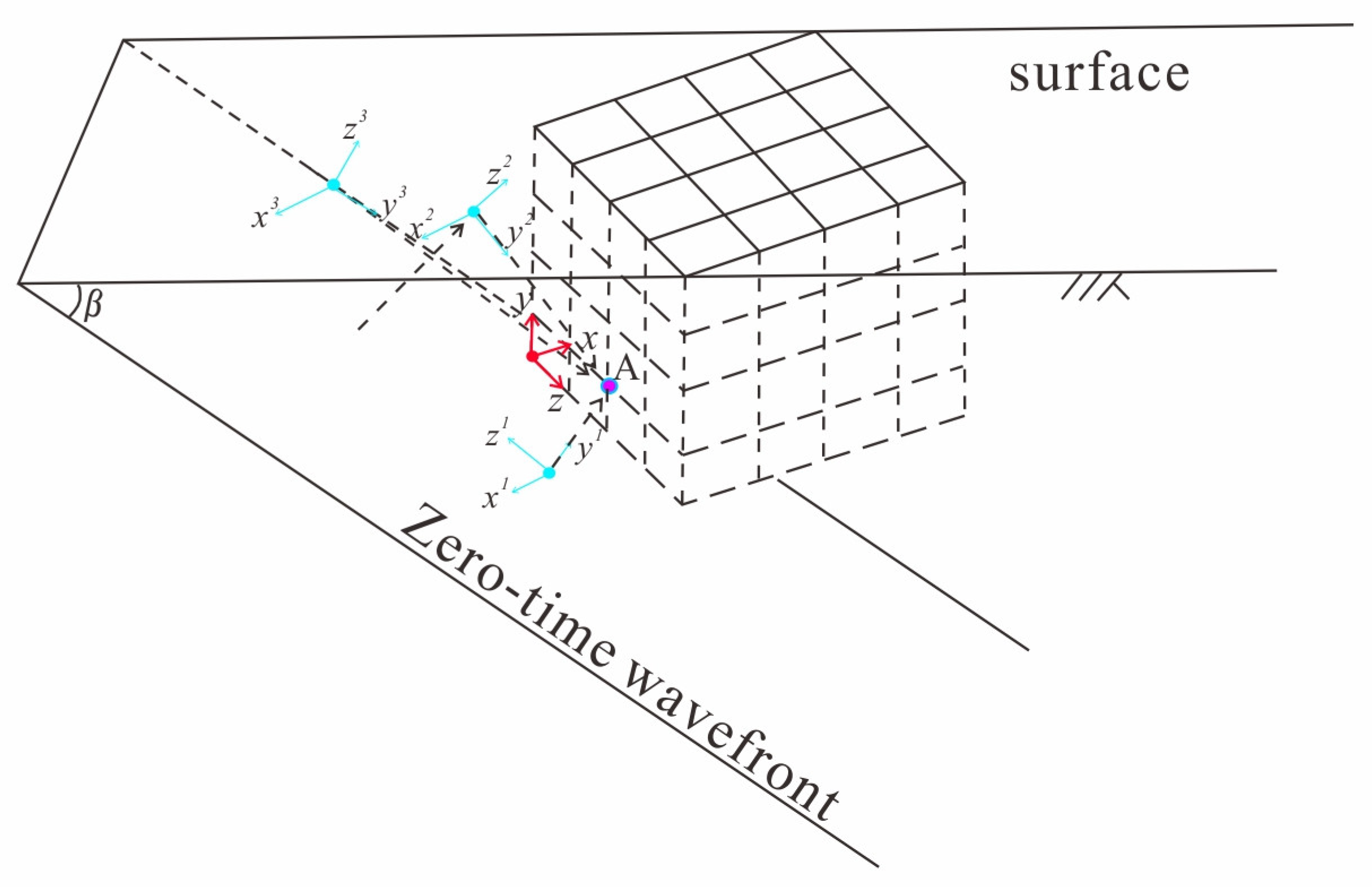
In a 3D coordinate system, a plane SV wave (with displacement time history u₀(t)) is assumed to impinge obliquely. A cubic artificial boundary is adopted, and an FE model is constructed through mesh discretization (Figure 1).

Taking one vertex of the cube as the origin, a global coordinate system is established, with the incident wavefront at the initial moment passing through point O. For an arbitrary point A(x₀,y₀,z₀) on the artificial boundary, the free-field response induced by the incident SV wave consists of three components: the directly incident SV₁ wave from the initial wavefront, the surface-reflected SV₂ wave, and the surface-reflected P wave. Corresponding local coordinate systems are defined for these three waves as (x¹,y¹,z¹), (x²,y²,z²), and (x³,y³,z³), respectively. The propagation direction of the incident SV wave forms angles α, β, and γ with the x-, y-, and z-axes.

The transformation matrix from the local coordinate system (x¹,y¹,z¹) to the global coordinate system is expressed as follows:

$${\mathrm{T}}_1=\left|\begin{array}{ccc}-{\displaystyle \frac{cos\gamma }{\sqrt{{cos}^2\alpha +{cos}^2\gamma }}}& 0& {\displaystyle \frac{cos\alpha }{\sqrt{{cos}^2\alpha +{cos}^2\gamma }}}\\ cos\alpha & -cos\beta & cos\gamma \\ -{\displaystyle \frac{cos\alpha cos\beta }{\sqrt{{cos}^2\alpha +{cos}^2\gamma }}}& \sqrt{{cos}^2\alpha +{cos}^2\gamma }& -{\displaystyle \frac{cos\gamma cos\beta }{\sqrt{{cos}^2\alpha +{cos}^2\gamma }}}\end{array}\right|$$

(5)

The transformation matrix from the local coordinate system (x²,y²,z²) to the global coordinate system is as follows:

$${\mathrm{T}}_2=\left|\begin{array}{ccc}-{\displaystyle \frac{cos\gamma }{\sqrt{{cos}^2\alpha +{cos}^2\gamma }}}& 0& {\displaystyle \frac{cos\alpha }{\sqrt{{cos}^2\alpha +{cos}^2\gamma }}}\\ cos\alpha & -cos\beta & cos\gamma \\ {\displaystyle \frac{cos\alpha cos\beta }{\sqrt{{cos}^2\alpha +{cos}^2\gamma }}}& \sqrt{{cos}^2\alpha +{cos}^2\gamma }& {\displaystyle \frac{cos\gamma cos\beta }{\sqrt{{cos}^2\alpha +{cos}^2\gamma }}}\end{array}\right|$$

(6)

The transformation matrix from the local coordinate system (x³,y³,z³) to the global coordinate system is the following:

$${\mathrm{T}}_3=\left|\begin{array}{ccc}-{\displaystyle \frac{cos{\gamma }_P}{\sqrt{{cos}^2{\alpha }_P+{cos}^2{\gamma }_P}}}& 0& {\displaystyle \frac{cos{\alpha }_s}{\sqrt{{cos}^2{\alpha }_s+{cos}^2{\gamma }_s}}}\\ cos{\alpha }_P& -cos{\beta }_P& cos{\gamma }_P\\ -{\displaystyle \frac{cos{\alpha }_{P}cos{\beta }_P}{\sqrt{{cos}^2{\alpha }_P+{cos}^2{\gamma }_P}}}& \sqrt{{cos}^2{\alpha }_P+{cos}^2{\gamma }_P}& -{\displaystyle \frac{cos{\gamma }_{P}cos{\beta }_P}{\sqrt{{cos}^2{\alpha }_P+{cos}^2{\gamma }_P}}}\end{array}\right|$$

(7)

where ${\beta }_p=arcsin\left({\displaystyle \frac{c_{P}sin\beta }{c_s}}\right), {\alpha }_P=arccos\left({\displaystyle \frac{cos\alpha sin{\beta }_P}{sin\beta }}\right), \mathrm{a}\mathrm{n}\mathrm{d} {\gamma }_P=arccos\left({\displaystyle \frac{cos\gamma sin{\beta }_p}{sin\beta }}\right)$.

In the local coordinate systems, the displacement components at point A, induced by the SV₁, SV₂, and P waves can be expressed as follows:

$$\left[U^1\right]=\left[\begin{array}{ccc}0& 0& u(t-△t^1)\end{array}\right]$$

(8)

$$\left[U^2\right]=\left[\begin{array}{ccc}0& 0& A_{3}u(t-△t^2)\end{array}\right]$$

(9)

$$\left[U^3\right]=\left[\begin{array}{ccc}0& A_{4}u(t-△t^3)& 0\end{array}\right]$$

(10)

where $△t^1~△t^3$ denote the time delays, which are obtained as follows:

$$△t^1={\displaystyle \frac{\left|x_{0}cos\alpha +y_{0}cos\beta +Z_{0}cos\gamma \right|}{c_s}}$$

(11)

$$△t^2={\displaystyle \frac{\left|x_{0}cos\alpha +(Ly-y_0)cos\beta +Z_{0}cos\gamma \right|}{c_s}}$$

(12)

$$△t^3={\displaystyle \frac{\left|(x_0-(Ly-y_0)cos{\alpha }_P/cos{\beta }_P)cos\alpha +Lycos\beta +(Z_0-(Ly-y_0)cos{\gamma }_p/cos{\beta }_P)\right|}{c_s}}+{\displaystyle \frac{(Ly-y_0)/cos{\beta }_P}{c_P}}$$

(13)

Using the transformation matrices, the displacement vector at point A in the global coordinate system is obtained by superposing the free-field contributions from the SV₁, SV₂, and P waves, which can be expressed as follows:

$$\left[U\right]={\displaystyle \sum _{i=1}^3}{T}_i\left[U_i\right]$$

(14)

The velocity vector in the global coordinate system is obtained by differentiating Equation (14) with respect to time:

$$\left[\dot{U}\right]={\displaystyle \sum _{i=1}^3}{T}_i\left[{\dot{U}}_i\right]$$

(15)

In the local coordinate system, the free-field stresses at point A caused by the SV₁ and SV₂ are obtained as follows:

$$\left[{\sigma }_{ij}^l\right]=\left[\begin{array}{ccc}0& 0& 0\\ 0& 0& {\tau }_{yz}^l\\ 0& {\tau }_{zy}^l& 0\end{array}\right], {\tau }_{yz}^l={\tau }_{zy}^l=-{\displaystyle \frac{G}{c_s}}u(t-△t^l)$$

(16)

where i = 1 and 2 denote the cases of the SV₁ and SV₂ waves, respectively.

In the local coordinate system, the free-field stress at point A due to the P wave is obtained as follows:

$$\left[{\sigma }_{ij}^l\right]=\left[\begin{array}{ccc}{\sigma }_{xx}^3& 0& 0\\ 0& {\sigma }_{yy}^3& 0\\ 0& 0& {\sigma }_{zz}^3\end{array}\right], {\sigma }_{xx}^3={\sigma }_{zz}^3=-{\displaystyle \frac{\lambda }{c_P}}\dot{u}(t-△t^3), {\sigma }_{yy}^3=-{\displaystyle \frac{\lambda +2G}{c_P}}\dot{u}(t-△t^3)$$

(17)

In the global coordinate system, the free-field stress at point A is expressed by superposing the contributions from the SV₁, SV₂, and P waves, expressed as follows:

$$\left[{\sigma }_{ij}^l\right]={\displaystyle \sum _{l=1}^2}{\left[T_l\right]}^T\left[{\sigma }_{ij}^l\right]\left[T_l\right]$$

(18)

Substituting Equations (14), (15) and (18) into Equation (17) yields the dynamic equation for 3D SV wave incidence.

2.2. Verification of Seismic Input Method

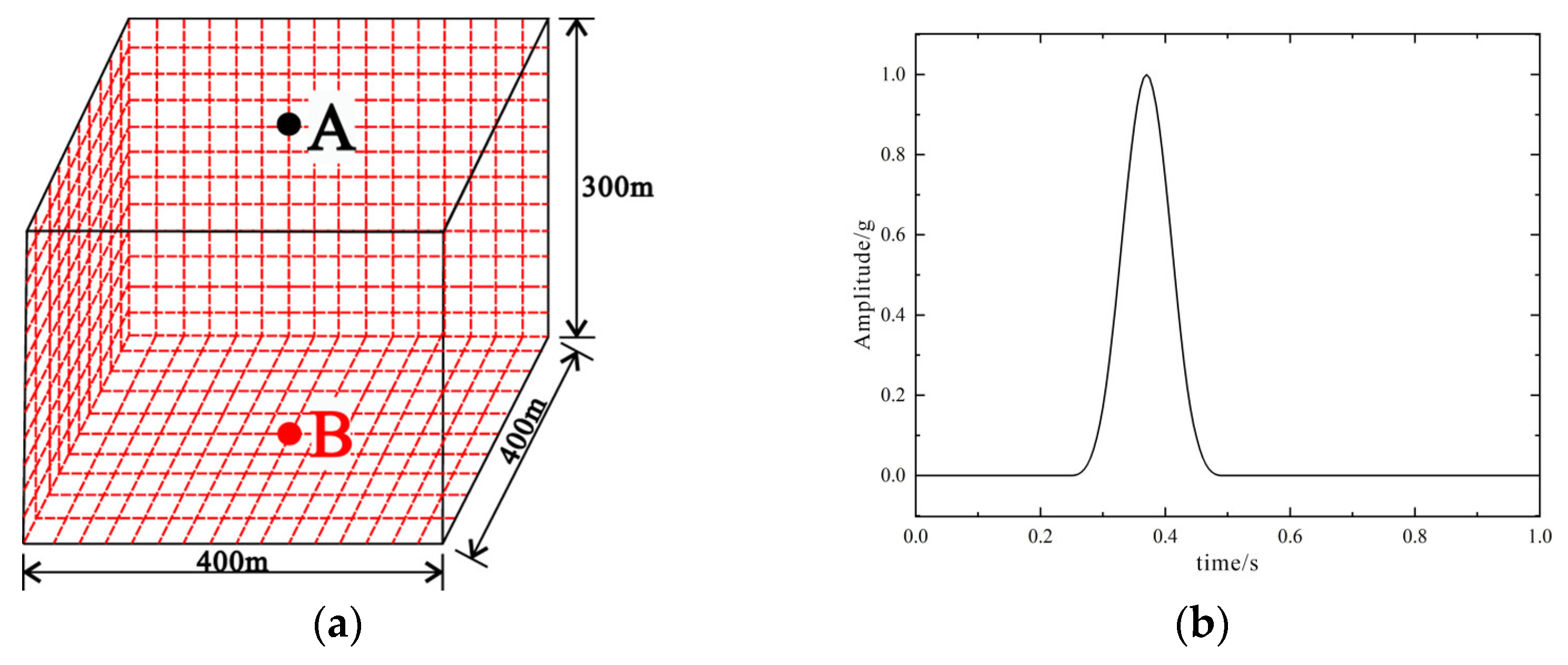
To evaluate the accuracy of the proposed 3D SV wave input approach, the dynamic response of a homogeneous elastic half-space subjected to obliquely incident plane SV waves was analyzed. The medium had a density of 2000 kg/m³, an elastic modulus of 1000 MPa, and a Poisson’s ratio of 0.2. The ABAQUS finite element software was selected to analyze the input method. In the finite element analysis (FEA), a rectangular domain of 400 × 400 × 300 m was employed. The grid size must be less than 1/10 of the wavelength, and, in this paper, the grid size was set to 5 m to ensure both the computational accuracy and efficiency. The corresponding FE model is illustrated in Figure 2a.

Viscoelastic boundaries were applied to the lateral and bottom surfaces of the FE model. To ensure the stability and accuracy of the numerical calculation, the step size was set to match the input wave; a time step of 0.005 s was adopted for time integration; the incident SV wave was defined as a Heaviside pulse, with a peak amplitude of 1 m and a duration of 0.25 s (see as Figure 2b). The propagation directions of the SV waves were specified by the vectors (tan 15°, 1, 0) and (tan 25°, 1, 0).

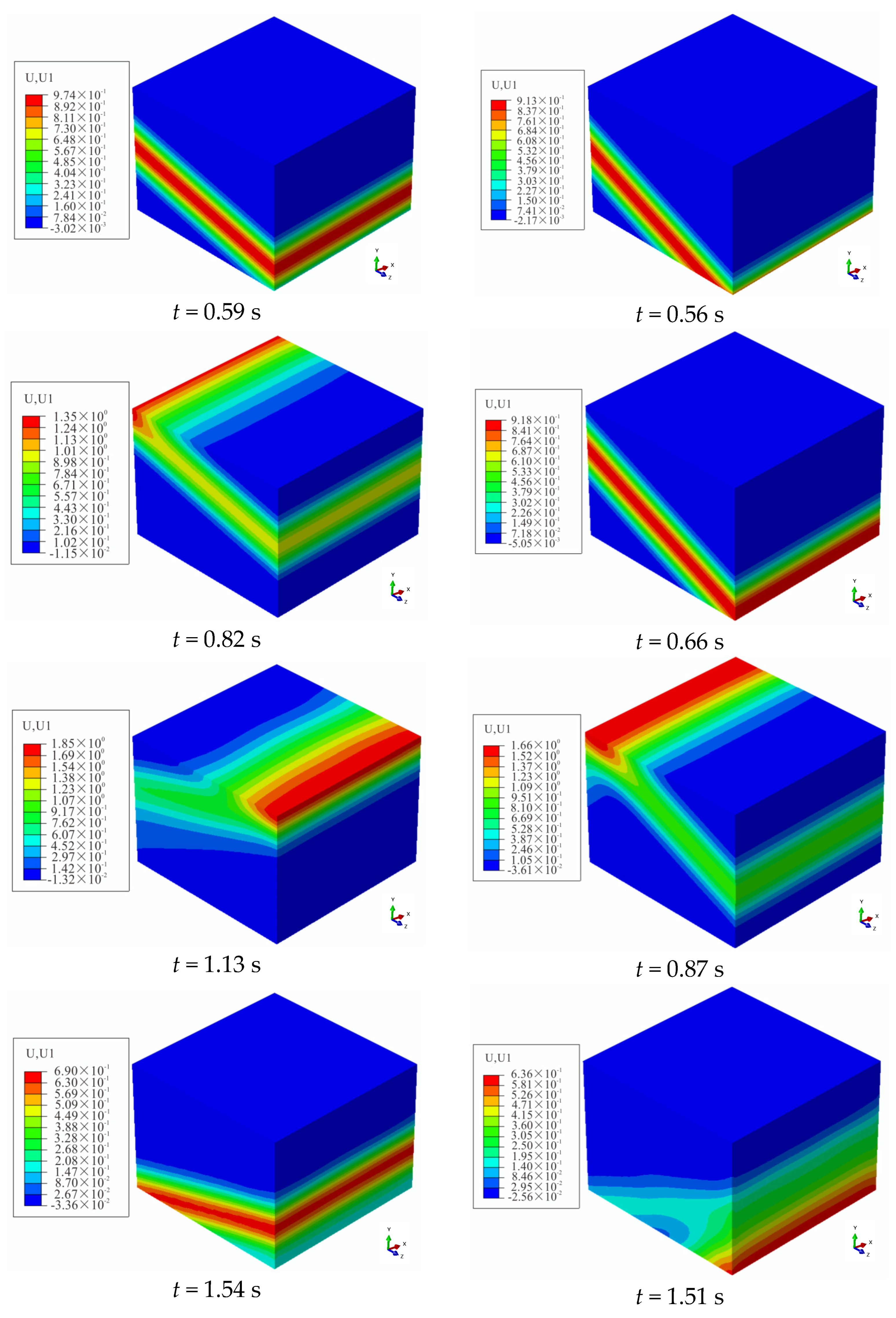
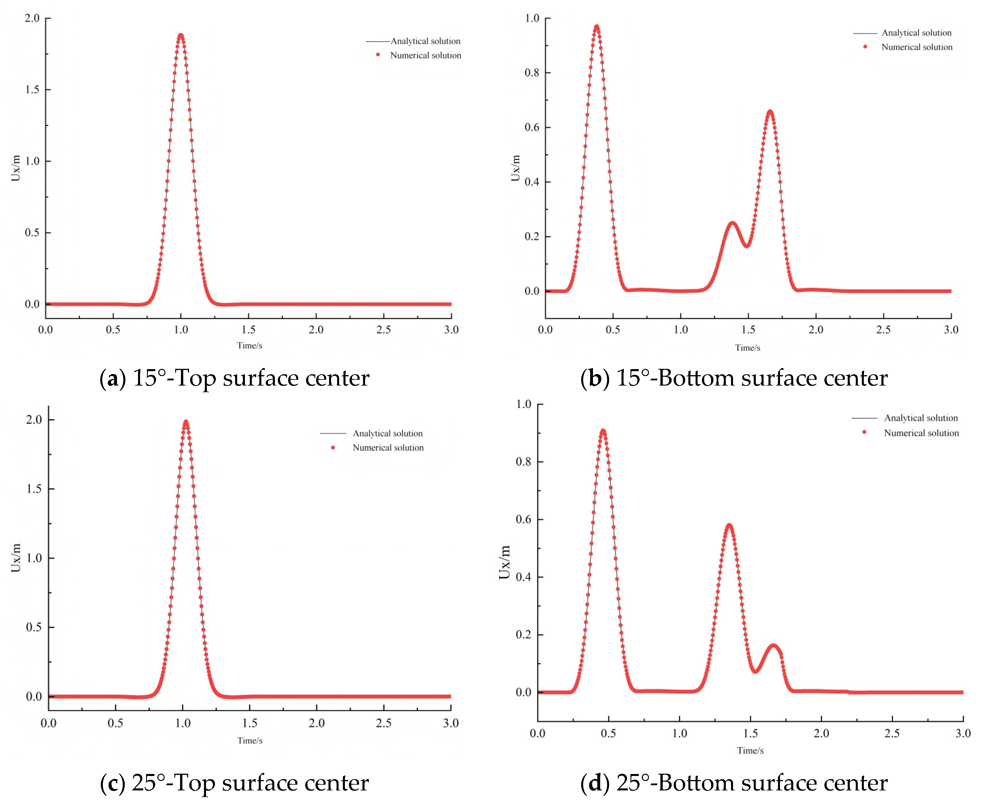
Figure 3 depicts the displacement contours of the half-space under two SV wave incident angles. The results indicate that the proposed input method accurately captures the propagation characteristics of SV waves in the half-space. Figure 4 presents the horizontal u0(t) at point B (center of the bottom surface) and point A (center of the top surface) for the two incident angles. A close agreement between the numerical and theoretical solutions can be observed, demonstrating the reliability of the proposed method.

2.3. Three-Dimensional Tunnel Model

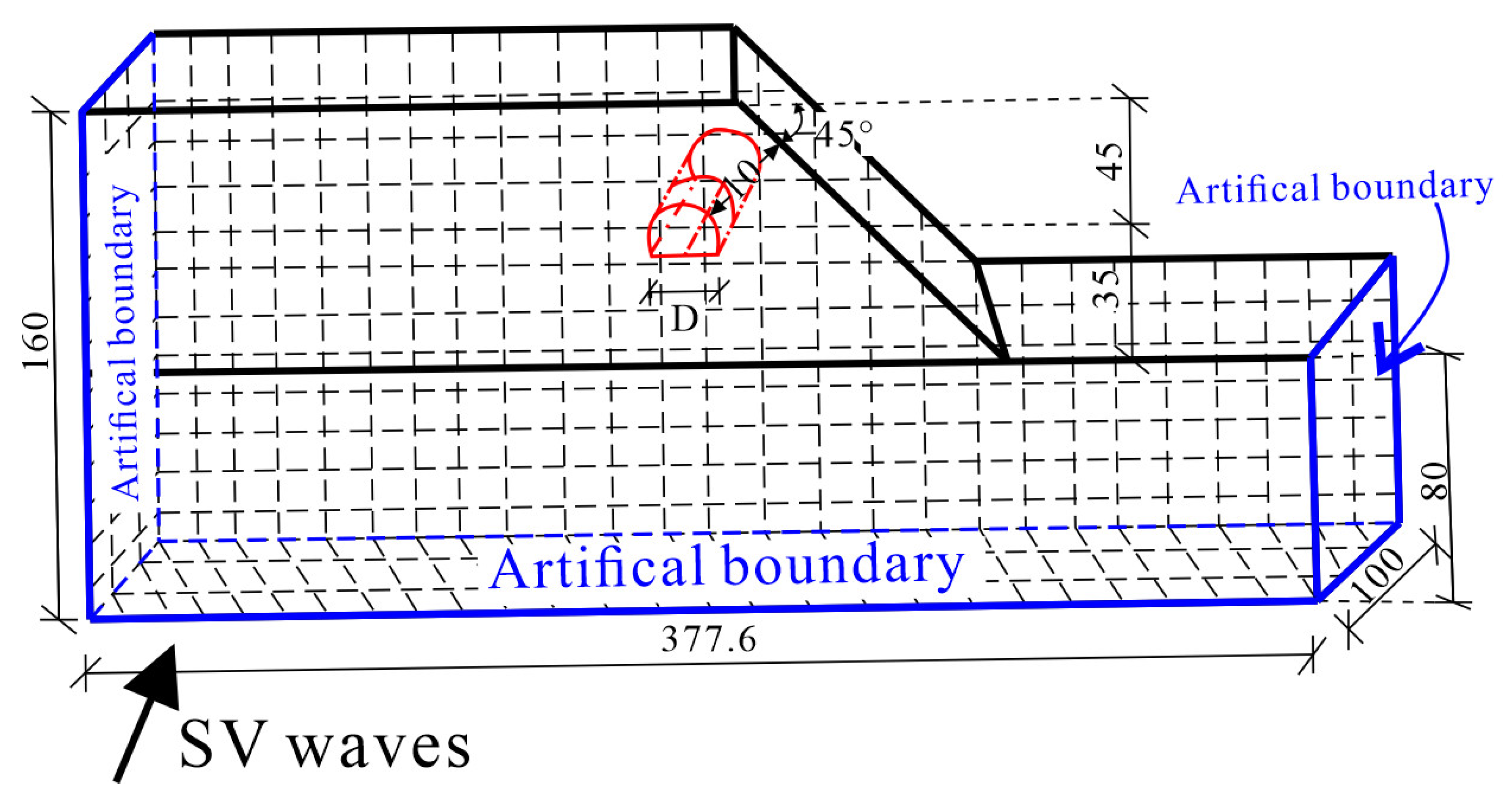
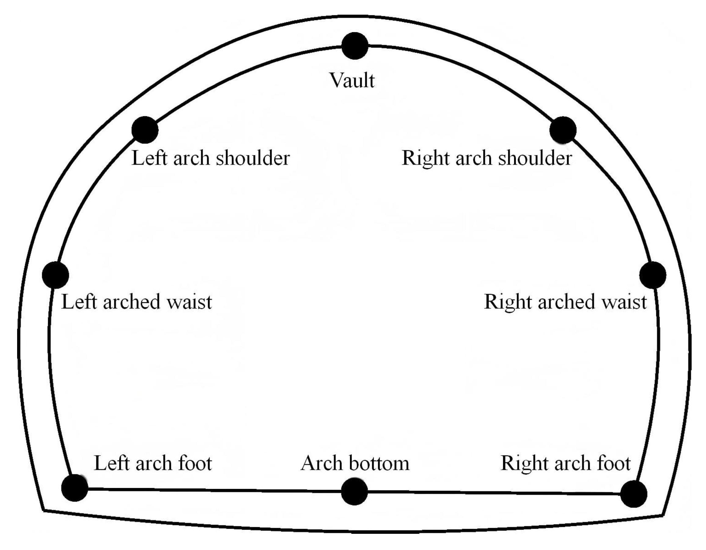
Based on the geological conditions of a tunnel along the Chengdu–Lanzhou Railway, a 3D integrated model of the surrounding rock and a biased tunnel was established (Figure 5). The surrounding rock was classified as Grade V; the maximum tunnel span was D = 11.8 m, with a height of 9.86 m, a tunnel spacing of A = 4D, and a lining thickness of 0.5 m. Following the model dimensions reported in Zhou et al. [19], the left and right boundary heights were set to 160 m and 80 m, respectively, with a bias angle of 45° and an overburden thickness of 10 m. The key characteristic points of the tunnel lining are illustrated in Figure 6. Obliquely incident seismic waves were assumed to enter the computational domain from the left boundary. The main calculation parameters are summarized in

Table 1. Material parameters of proposed model.

Material	Density (kg/m3)	Elastic Modulus (GPa)	Poisson’s Ratio	Cohesion (kPa)	Internal Friction Angle (°)
Surrounding rock	2400	2.3	0.3	-	-
Tunnel	2200	1.0	0.2	150	30

. According to Liao et al. [34], accurate simulation of seismic wave propagation requires the mesh size to be smaller than one-tenth to one-eighth of the wavelength corresponding to the highest frequency component of the input wave.

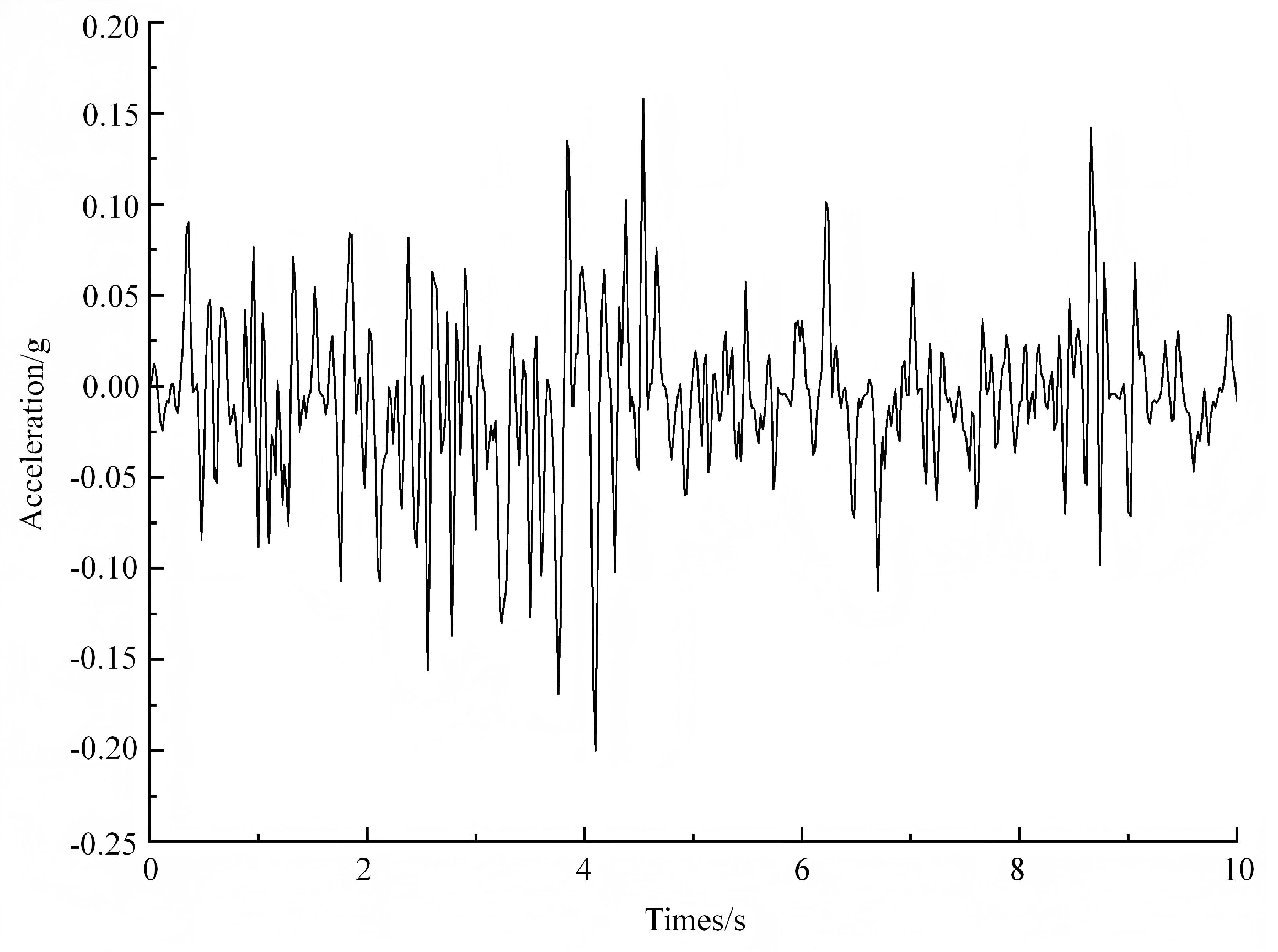
Based on Equation (18) and the formation parameters, the critical incident angle of the SV wave was determined to be 32°. Compressive considering efficiency and analysis, the influence of the incident angles was set as 5° intervals in this study. The incident angles α are 0° (vertical incidence), 5°, 10°, 15°, 20°, and 25°. The Wenchuan seismic record was selected as the input motion. To reduce computational cost, a 20 s time window centered around the peak acceleration (10 s before and after) was extracted, with a time step of 0.02 s. According to the seismic fortification intensity and site conditions, the input motion was scaled to 0.2 g. The resulting acceleration time–history curve is depicted in Figure 7.

3. Results and Analysis

3.1. Stress Analysis of Biased Tunnel

The dynamic responses of the shallow-buried biased tunnel were evaluated for α of 0° (vertical), 5°, 10°, 15°, 20°, and 25°, with the aim of examining the variation in tunnel stress under different incidence conditions.

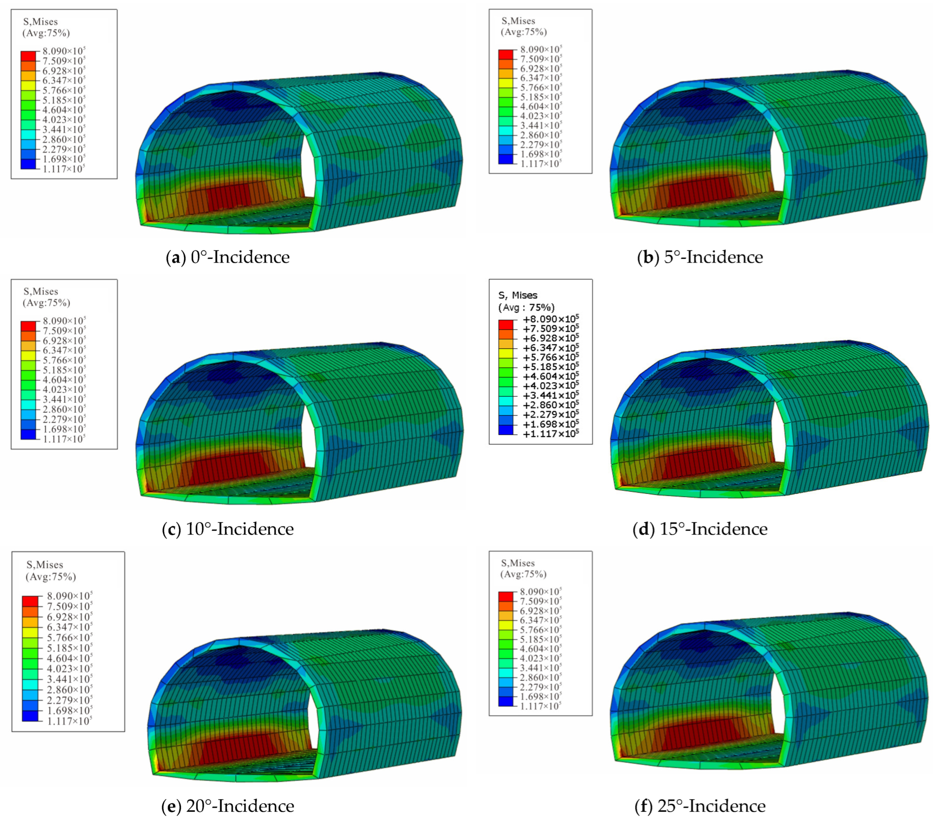
The stress patterns in Figure 8 show that, for obliquely incident SV waves, stresses are concentrated near the left arch foot of the tunnel, a distribution which remains largely unchanged across different α values, indicating that this region acts as a consistently vulnerable zone in shallow-buried biased tunnels. The concentration is attributed to the superposition of seismic-induced dynamic responses in this area. In terms of magnitude, vertical α (0°) produces relatively low peak stress, suggesting limited dynamic amplification when the wavefront is perpendicular to the tunnel axis. As α increases, the peak stress rises by approximately 3%. Beyond 15°, the increase becomes negligible and the stress level stabilizes with only minor variation. Overall, the peak stress increases initially and then approaches a steady state as α grows.

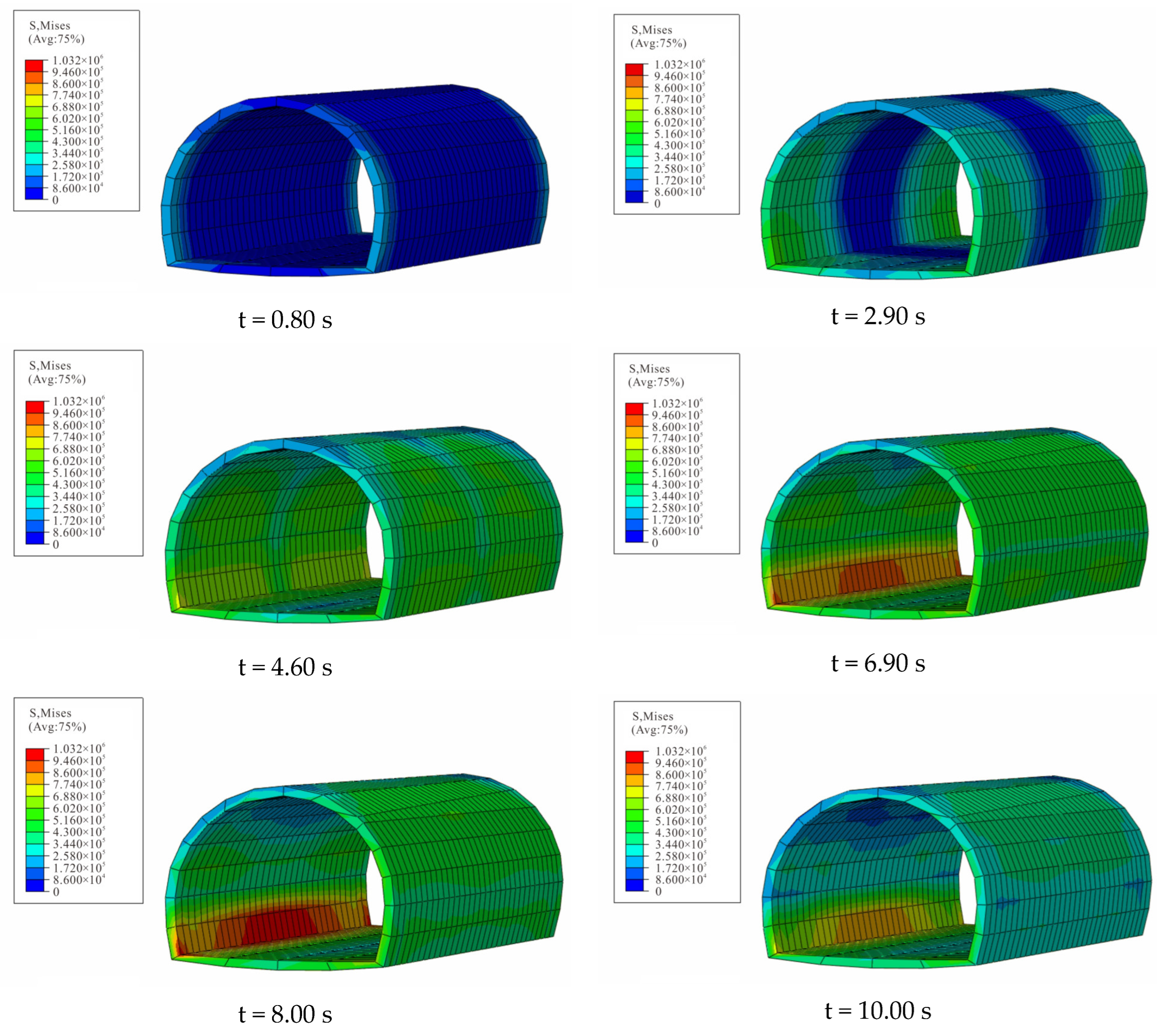
In Figure 8, the stress variation in the shallow-buried biased tunnel exhibits a similar developmental trend under different α. To further investigate the stress evolution at different time stages under obliquely incident seismic waves, the case of α at 15° was selected, and the corresponding stress contours at different times were analyzed (Figure 9).

The stress evolution contours in Figure 9 show that the dynamic stress response of the shallow-buried biased tunnel follows a four-stage pattern, namely “local initiation–biased-side concentration–global peak–gradual dissipation”, a process consistently governed by the coupled effects of biased topography and wave incidence direction. The stress distribution characteristics and their evolution at each stage are described as follows:

During the initial stage (t = 0~0.8 s), the stress field exhibits localized initiation behavior, with stress concentration first appearing near the tunnel portals. The stress levels at the arch foot and shoulder are noticeably higher than in other regions, while the crown remains at a relatively low level. At t ≈ 2.9 s, the stress field enters a propagation stage, with the initially concentrated stress at the tunnel portals extending toward the interior. As seismic energy continues to accumulate, stress progressively concentrates toward the left arch foot. When t ≈ 4.6 s, a clear spatial asymmetry develops, with lower stress levels at the crown and at the right arch foot compared to the left, indicating the emergence of biased effects. By t ≈ 6.9 s, a pronounced stress concentration forms at the left arch foot in the central section of the tunnel, and the high-stress zones on the biased side become fully connected, marking the transition to the biased-side concentration stage. At approximately 8 s, the stress field reaches its peak state over the entire time history, with both the extent and intensity of concentration attaining maximum values; the peak stress is 1.032 MPa. At t = 10.0 s, the stress field enters a dissipation stage and gradually stabilizes. The stress at the biased-side arch foot decreases to 0.809 MPa, representing a reduction of 21.61% compared with the peak value. Thereafter, the stress distribution shows no significant further change, and the overall evolution process of the tunnel stress field is characterized by the four-stage pattern of “local initiation–biased-side concentration–global peak–gradual dissipation”. As shown from the time-domain of stress, the stress distribution appears asymmetric characteristics. Stress concentrate at the foot, shoulder of the tunnel firstly, then, extend to the deep of the tunnel. The same stress distribution is also illustrated by Shi [35].

3.2. Acceleration Analysis of Biased Tunnel

The dynamic responses of the shallow-buried biased tunnel are computed for α of 0° (vertical), 5°, 10°, 15°, 20°, and 25°, in order to investigate how the acceleration response of the tunnel varies with the α.

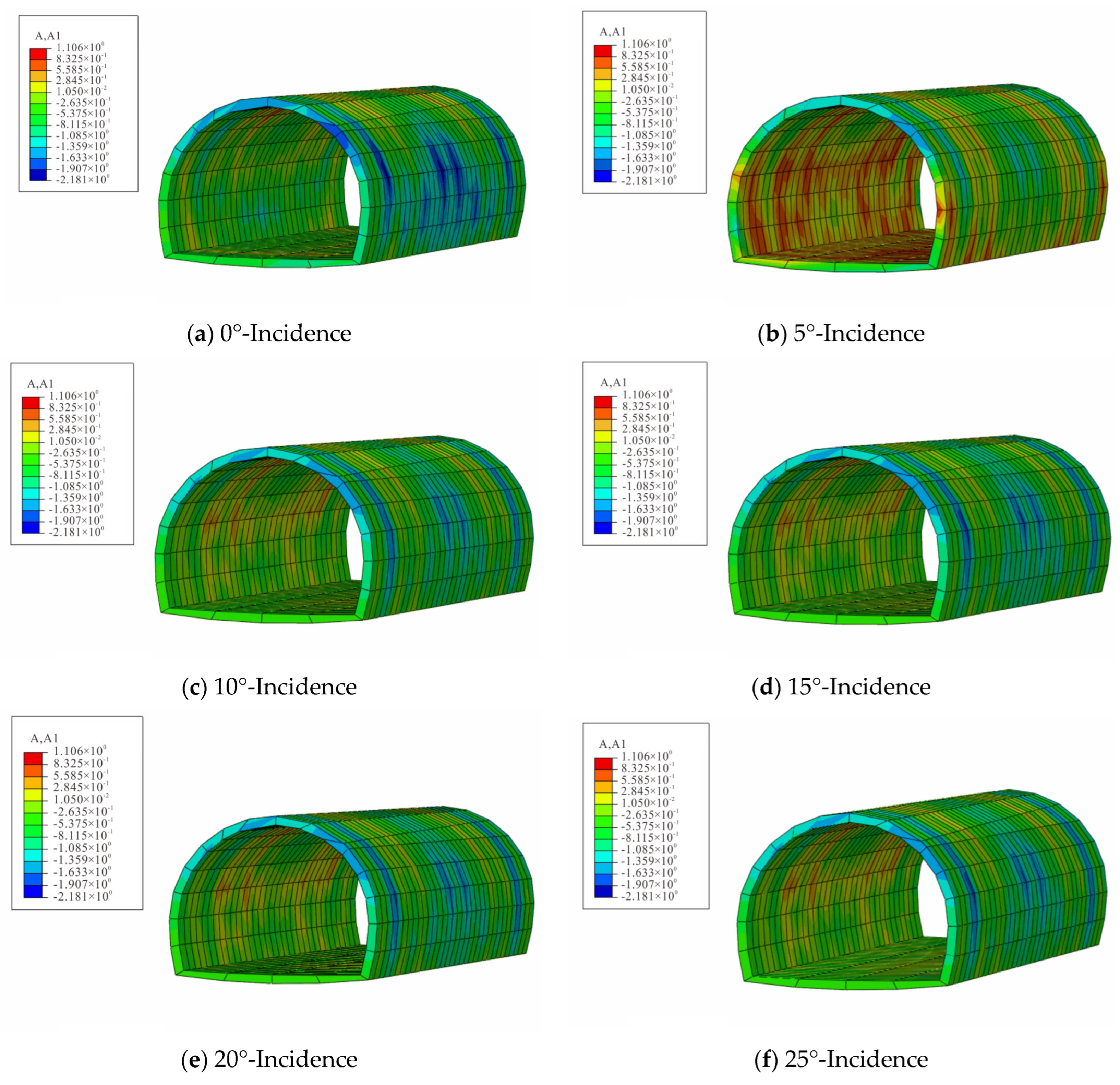
The acceleration distributions under different α values (Figure 10) indicate that, under biased conditions, the acceleration is predominantly concentrated near the left arch foot of the tunnel. For various values of α, the acceleration response of the tunnel structure exhibits distinct characteristics. Under vertical SV wave incidence, higher acceleration values are mainly observed around the arch shoulder and crown. With increasing α, the region of elevated acceleration gradually shifts toward the left arch foot and eventually becomes concentrated in that area. In addition, to better capture the temporal variation in acceleration, the evolution process corresponding to α = 15° is illustrated in Figure 10.

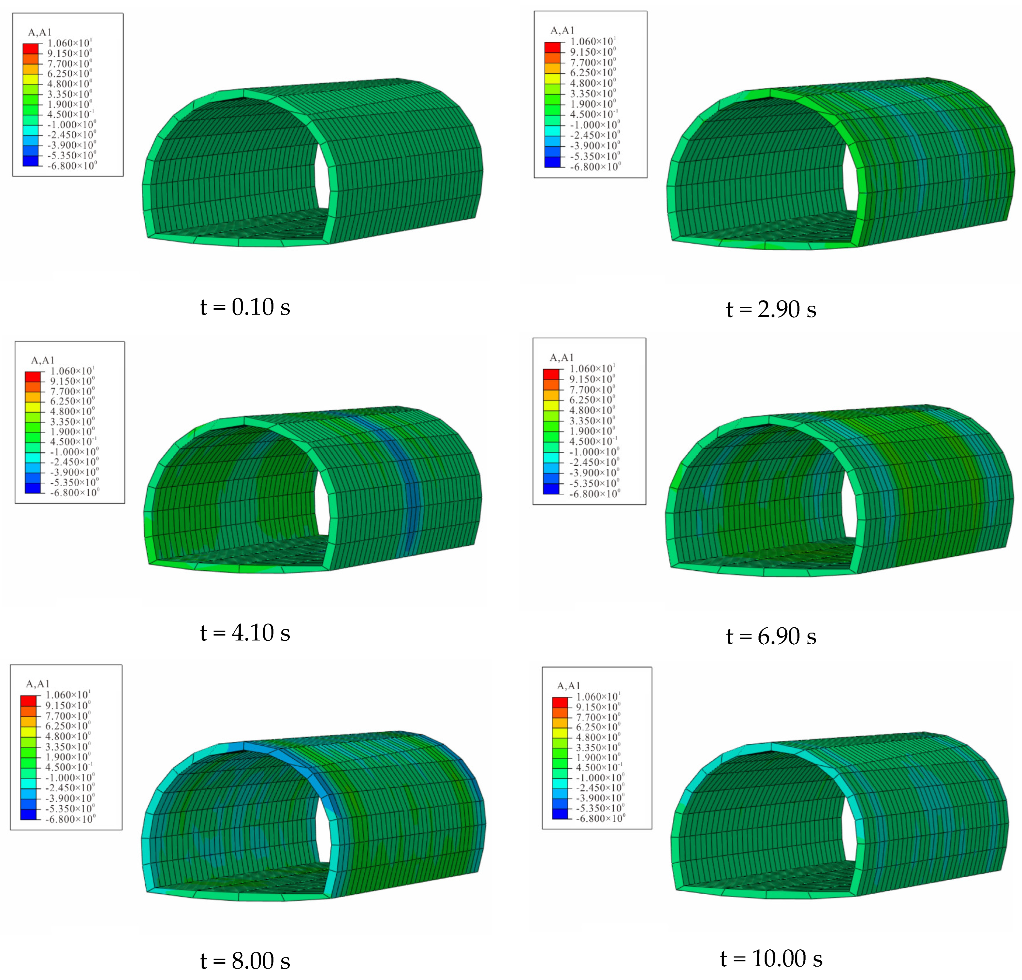
The acceleration evolution in Figure 11 reveals that the dynamic response of the shallow-buried biased tunnel can be divided into four characteristic stages: the initial response stage, the wave propagation and reflection stage, the intensified interaction stage, and the stable vibration and attenuation stage. The evolution process is governed by the combined influence of biased topography and the direction of stress-wave incidence, and the characteristics of each stage are described as follows:

At t = 0.10 s, corresponding to the initial stage, the SV wavefront reaches the tunnel structure, and the dynamic response is in its early excitation phase. Since wave energy has not yet undergone sufficient reflection or superposition within the structure, the acceleration fields of both the tunnel and surrounding rock remain relatively uniform. The peak acceleration is mainly located in the arch shoulder region or in the surrounding rock outside the sidewall where the wavefront first arrives. The acceleration shows a tendency to propagate outward from the central surrounding rock toward both sides, while the structural response of the tunnel itself is still limited. During the interval t = 2.90~4.10 s, the shallow-buried biased effect becomes more pronounced, leading to the development of an asymmetric acceleration field. Peak acceleration appears in the surrounding rock above the crown on the shallow-buried side and near the arch shoulder on the same side, reflecting zones where stress waves tend to converge and interact with the biased topography. Between t = 4.10 and 6.90 s, the peak acceleration increases significantly, which is attributed to wave reflection and scattering within the strata, with an amplitude increase of 94.11%. Meanwhile, the location of peak acceleration shifts. In addition to the crown and the arch shoulder on the shallow-buried side remaining dominant response regions, high-acceleration zones extend toward the invert or the sidewall foot on the deeply buried side, indicating that dynamic interaction reaches its most intense stage. During t = 6.90~10.00 s, the peak acceleration decreases to some extent, and its location stabilizes near the junction of the crown and sidewall. As the external wave input weakens, the overall seismic response transitions into a stage of attenuated vibration. The evolution of the acceleration field reflects a complete process in which energy gradually redistributes, from concentration to dissipation, and from global excitation to more localized vibration. As shown from the acceleration, the evolution of the acceleration is “excitation–bias accentuation–intense interaction”. It revealed that the pattern of the acceleration distribution is driven by the “topography-wave propagation”. The key point of the asymmetric distribution of acceleration is influenced by the biased topography and the wave propagation.

3.3. Tunnel Damage Evolution

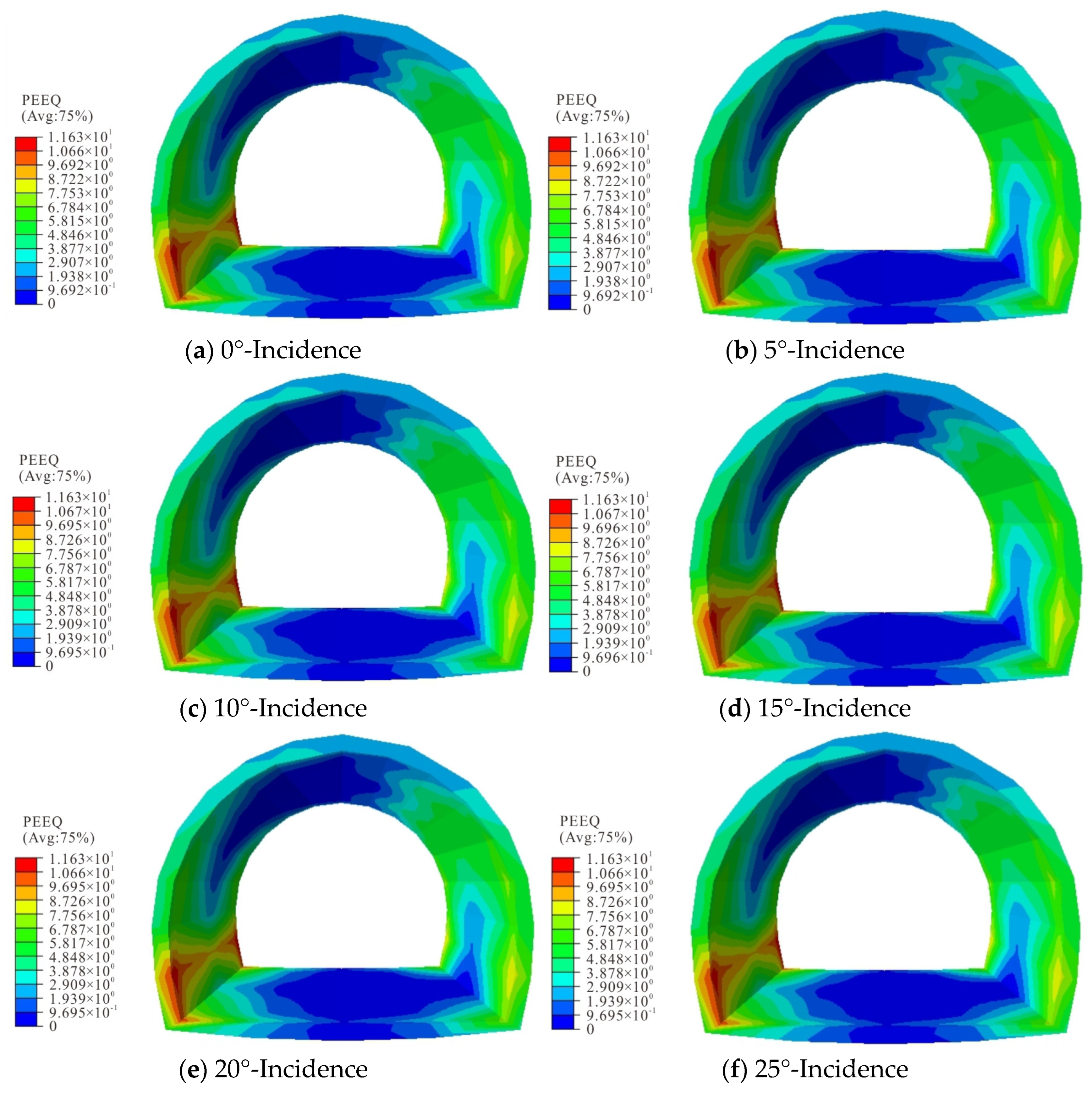
The dynamic responses of the shallow-buried biased tunnel are obtained for α values of 0° (vertical), 5°, 10°, 15°, 20°, and 25°, with a focus on characterizing the variation in tunnel damage under different incidence conditions. The equivalent plastic strain (PEEQ) is used to describe the damage evolution.

The damage distribution patterns under different values of α (Figure 12) reveal that, for obliquely incident SV waves, damage is primarily concentrated at the left arch foot of the tunnel, forming a continuous and penetrating damage zone. Despite variations in α, the overall damage distribution remains similar, indicating that this region constitutes a typical weak zone of shallow-buried biased tunnels, a phenomenon associated with the accumulation of seismic-induced dynamic effects in this area, which promotes the progression of local damage. From a quantitative perspective, the peak plastic strain is about 11.63% for varying α, with only minor fluctuations. Under vertical α (0°), the minimum damage is relatively low. As α increases, the minimum damage shows a stage-dependent increase, rising by about 2.5% compared with the vertical case in the initial stage. When α exceeds 10°, the minimum damage stabilizes at approximately 4.698 with limited variation. Overall, the minimum damage exhibits a trend of initial growth followed by stabilization as α increases.

As shown from the results, the directional damage concentration of biased tunnel under obliquely incident SV waves is indicated, a finding that breaks from the understanding of the damage suffered in tunnels being “scattered throughout the structure”. The left feet of the tunnel are weak under oblique seismic waves, the reason for which is illustrated as follows: the superposition effect is enhanced in this region due to the propagation of the incident and reflect waves.

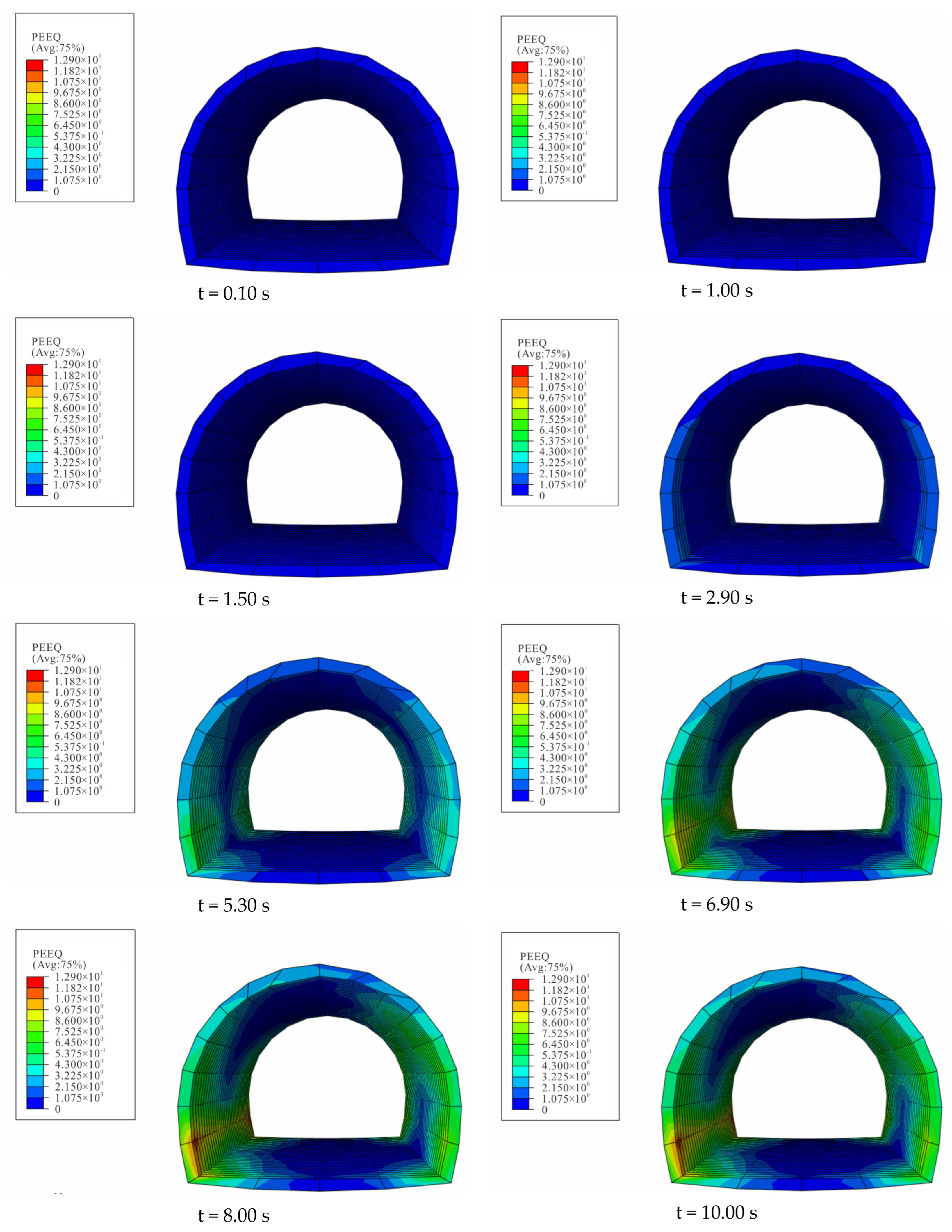
Regarding the damage evolution of a single tunnel under obliquely incident SV waves, the process follows a four-stage pattern (Figure 13): “no obvious initial damage → local damage initiation → accelerated damage propagation → stable damage development”, as detailed below:

At t = 0.8 s, damage begins to initiate, mainly concentrated at the arch foot, where stress concentration is prominent, accompanied by the formation of localized microcracks. At t = 1.0 s, the plastic damage zone starts to extend toward the arch waist, while the seismic loading has not yet caused significant deterioration to the tunnel structure or the surrounding rock. By t = 1.5 s, the plastic damage further develops toward the arch shoulder, forming a localized zone of plastic strain concentration, whereas the crown remains relatively intact without noticeable damage. When t = 2.9 s, the affected region expands, with the plastic strain concentration at the arch foot extending slightly into the deeper surrounding rock, and the damage at the biased-side arch waist becoming more distinct. However, the overall damage level remains limited, and no continuous damage band has yet formed, indicating that the structural stability is not significantly compromised. As t = 5.30 s, the initially localized damage undergoes marked expansion: the plastic strain zone at the arch foot propagates deeper into the surrounding rock and spreads toward the invert, while the damage at the biased-side arch waist enlarges and gradually approaches that at the arch foot. In addition, slight plastic strain concentration is observed at the crown for the first time. By t = 6.90 s, the damage zones at the arch waist and arch foot on the biased side become fully connected, forming a longitudinal damage band along the biased side of the tunnel; meanwhile, the damage at the crown intensifies, and the plastic strain increases significantly. The damage pattern evolves from localized development to a coordinated multi-zone state involving the crown, arch waist, and arch foot, accompanied by a noticeable reduction in structural load-bearing capacity. At t = 8.0 s, the damage continues to develop, but tends toward a stable configuration, and the overall damage pattern of the tunnel becomes well established. Finally, when t = 10.00 s, the damage state remains essentially unchanged, with no significant variation in the distribution of plastic strain. The tunnel ultimately reaches a stable damage configuration, characterized by a continuous damage band along the biased-side arch waist and arch foot, together with localized damage at the crown, indicating that the damage evolution process has effectively completed.

In summary, under obliquely incident SV waves, stress in a shallow-buried biased tunnel is primarily concentrated at the left arch foot, while plastic damage tends to initiate in stress concentration regions, such as the biased-side arch waist and arch foot. The nonuniform stress distribution induced by biased loading conditions plays a key role in controlling both the location and progression of damage. Meanwhile, this study indicated that the damage of the biased tunnel follows a step-by-step progression, which provides a “phased protection” in the seismic events. Furthermore, it indicates the triggering mechanisms of damage in multiple regions, i.e., arch shoulder, waist, and foot. The same damage distribution is also illustrated by Chen [36].

4. Conclusions

This study investigates the seismic response of a biased tunnel by establishing a numerical model based on a viscoelastic artificial boundary combined with equivalent seismic loads. The seismic behavior of the shallow-buried biased tunnel is examined from three perspectives, namely stress, acceleration, and plastic damage. The main conclusions are summarized as follows:

• The 3D seismic input method incorporating viscoelastic artificial boundaries and equivalent seismic loads demonstrates both high computational efficiency and accuracy. Comparison with theoretical solutions confirms the validity of the proposed approach.
• With an increasing seismic wave incident angle, stress tends to concentrate at the left arch foot, a behavior which is influenced not only by the incident angle, but also by the weight of the overlying rock mass under biased conditions. The plastic damage initiates near the arch shoulder and progressively develops toward the left arch foot, where it eventually concentrates. Therefore, for a tunnel located near a seismic source, the actual direction of the seismic waves must be taken into account. An appropriate reinforcement should be applied to the arch foot on the side close to the source in order to resist the influence of obliquely incident seismic waves.

References

1. Shi, W.; Xu, Y.; Lin, G. Simplification of earthquake induced vehicle bridge interaction contact simulation for urban viaducts. Earthq. Eng. Struct. Dyn. 2023, 52, 957–980. [Google Scholar] [CrossRef] [Scilit]
2. Kawashima, K. Seismic performance of RC bridge piers in Japan: An evaluation after the 1995 Hyogo-ken nanbu earthquake. Prog. Struct. Eng. Mater. 2000, 2, 82–91. [Google Scholar] [CrossRef] [Scilit]
3. Lu, C.-C.; Hwang, J.-H. Damage analysis of the new Sanyi railway tunnel in the 1999 Chi-Chi earthquake: Necessity of second lining reinforcement. Tunn. Undergr. Space Technol. 2018, 73, 48–59. [Google Scholar] [CrossRef] [Scilit]
4. Yan, X.; Zhu, H.; Wang, Y. Several Characteristics of Seismic Response of Mountain-crossing Tunnels. Tunn. Constr. 2009, 29, 420–423. [Google Scholar]
5. Xu, H.; Li, T.B.; Wang, D.; Li, Y.S.; Lin, Z.H. Study of seismic responses of mountain tunnels with 3d shaking table model test. Chin. J. Rock Mech. Eng. 2013, 32, 1762–1771. [Google Scholar]
6. Tsinidis, G.; de Silva, F.; Anastasopoulos, I.; Bilotta, E.; Bobet, A.; Hashash, Y.M.; He, C.; Kampas, G.; Knappett, J.; Madabhushi, G.; et al. Seismic behaviour of tunnels: From experiments to analysis. Tunn. Undergr. Space Technol. 2020, 99, 103334. [Google Scholar] [CrossRef] [Scilit]
7. De Silva, F.; Fabozzi, S.; Nikitas, N.; Bilotta, N.; Fuentes, R. Seismic vulnerability of circular tunnels in sand. Géotechnique 2021, 71, 1056–1070. [Google Scholar] [CrossRef] [Scilit]
8. Huang, J.; Zhao, M.; Du, X. Non-linear seismic responses of tunnels within normal fault ground under obliquely incident P waves. Tunn. Undergr. Space Technol. 2017, 61, 26–39. [Google Scholar] [CrossRef] [Scilit]
9. Zhu, J.; Li, X.; Liang, J.W. Seismic responses of underground tunnels subjected to obliquely incident seismic waves by 2.5D FE-BE coupling method. Chin. J. Geotech. Eng. 2022, 44, 1846–1854. [Google Scholar]
10. Du, X.L.; Huang, J.Q.; Zhao, M.; Lin, J. Effect of oblique incidence of SV waves on seismic response of portal sections of rock tunnels. Chin. J. Geotech. Eng. 2014, 36, 1400–1406. [Google Scholar]
11. Peng, Z.; Cui, J.; Li, Y.-D. Effect of oblique incident angle of P-wave on submarine immersed tunnels. World Earthq. Eng. 2016, 32, 78–85. [Google Scholar]
12. Liu, Z.; Liu, J.; Pei, Q.; Yu, H.; Li, C.; Wu, C. Seismic response of tunnel near fault fracture zone under incident SV waves. Undergr. Space 2021, 6, 695–708. [Google Scholar] [CrossRef] [Scilit]
13. Liu, J.; Gu, Y.; Li, B.; Wang, Y. An efficient method for the dynamic interaction of open structure-foundation systems. China Civ. Eng. J. 2007, 1, 340–345. [Google Scholar] [CrossRef] [Scilit]
14. Xiaolong, Z.; Xiaojun, L.; Guoxing, C.; Zhenghua, Z. An improved method of the calculation of equivalent nodal forces in viscous-elastic artificial boundary. Chin. J. Theor. Appl. Mech. 2016, 48, 1126–1135. [Google Scholar]
15. Huang, D.; Wang, H.; Cen, H.; Zong, Z.; Liu, Q.; Tang, A.; Tao, X. A study on dynamic response of a utility tunnel in horizontal non-homogeneous site based on SV wave oblique incidence. J. Vib. Shock. 2024, 43, 190–203. [Google Scholar]
16. Wang, H.; Huang, D.; Xu, C.; Yu, C.; Cen, H.; Huaang, Z.; Tang, A. Vulnerability analysis of utility tunnel under oblique incidence of SV waves in horizontal non-homogeneous field based on IDA method. J. Vib. Shock. 2025, 44, 160–171. [Google Scholar]
17. van Hoorickx, C.; Schevenels, M.; Lombaert, G. Double wall barriers for the reduction of ground vibration transmission. Soil Dyn. Earthq. Eng. 2017, 97, 1–13. [Google Scholar] [CrossRef] [Scilit]
18. Zhang, Q.; Zhao, M.; Huang, J.; Du, X. Parameter Analysis on Seismic Response of Long Lined Tunnel by 2.5D Substructure Method. Appl. Sci. 2023, 13, 4593. [Google Scholar] [CrossRef] [Scilit]
19. Huang, J.; Du, X.; Tian, Z.M.; Jin, L.; Zhao, M. Effect of the oblique incidence of seismic sv waves on the seismic response of subway station structure. Eng. Mech. 2014, 31, 81–88. [Google Scholar]
20. Lyu, D.; Ma, S.; Yu, C.; Liu, C.; Wang, X.; Yang, B.; Xiao, M. Effects of oblique incidence of SV waves on nonlinear seismic response of a lined arched tunnel. Shock. Vib. 2020, 2020, 8093804. [Google Scholar] [CrossRef] [Scilit]
21. Zhenning, B.; Zhiying, Y.; Jianwen, L. Dynamic response of a mountain tunnel under plane P-SV waves. Earthq. Eng. Eng. Dyn. 2018, 38, 50–58. [Google Scholar]
22. Du, X.L.; Chen, W.; Li, L.; Li, L.Y. Preliminary Study of Time-Domain Seismic Response for Underground Structures to Obliquely Incident Seismic Waves. Technol. Earthq. Disaster Prev. 2007, 2, 290–296. [Google Scholar]
23. Zhou, X.; Zhang, Y.; He, Y.; Liu, Z. Seismic response analysis of immersed tube tunnel under oblique incidence of seismic SV waves. China Earthq. Eng. J. 2017, 39, 600–608. [Google Scholar]
24. Huang, W.Z.; He, C.; Xu, G.Y.; Li, B. Seismic Response of a Submarine Immersed Tunnel Under Oblique Incidence of SV Waves. Tunn. Constr. 2024, 44, 724–738. [Google Scholar]
25. Zhang, D.D.; Liu, Y.; Xiong, F.; Mei, Z.; Li, S. Seismic response analysis of rock tunnel near-portal under oblique incidence of P wave and SV wave. J. Vib. Shock. 2022, 41, 278–286. [Google Scholar]
26. Zhang, B.W.; Yan, S.H.; Yang, Y.D. Approximation method of tunnel longitudinal seismic analysis. Rock Soil Mech. 2012, 33, 2081–2088. [Google Scholar]
27. Lin, J.; Zhu, J.L.; Huang, S.L.; Xiao, Q.; Huang, Y.B.; Lei, S.D.; Zhou, P. Numerical study on tunnel deformation under local thickness reduction in tunnel linings and destruction prediction. Chin. J. Geotech. Eng. 2024, 46, 177–182. [Google Scholar]
28. Wang, F.; Song, Z.; Lu, T. Nonlinear seismic responses of a hydropower house under near-fault ground motions oblique input. J. Vib. Shock. 2020, 39, 63–73. [Google Scholar]
29. Liu, L.; Song, Z.; Wang, F.; Li, C.; Liu, S.; Liu, Y. Vulnerability analysis of asphalt concrete core dam under near-fault ground motion. J. Vib. Eng. 2025, 38, 1106–1118. [Google Scholar]
30. Chen, Z.R.; Song, D.Q.; Liu, X.L.; Wang, C.W.; Zhang, J.W. Seismic Dynamic Response Characteristics of a Layered Slope at Tunnel Entrance Using Shaking Table Test. Earth Sci. 2022, 47, 2069–2080. [Google Scholar]
31. Liang, J.; Luo, H.; Lee, V.W. Scattering of plane SH waves by a circular-archill with a circular tunnel. Acta Seismol. Sin. 2004, 26, 495–508. [Google Scholar]
32. Zhu, H.; Yan, S.H.; Sun, W.Y.; Ou, E.F.; Lin, J.C.; Wang, J.H. Seismic Response Analysis of Shallow-Buried Unsymmetrical-Loading Double Tunnel Under Oblique Incidence of Seismic Wave. J. Vib. Meas. Diagn. 2024, 44, 259–265+407. [Google Scholar]
33. Zhou, T.; Dong, C.; Li, S.; Fan, S. Seismic response of tunnels with damping layer under oblique incident SV waves. World Earthq. Eng. 2024, 40, 1–12. [Google Scholar]
34. Liao, Z.; Liu, J. Elastic waves in discrete grids (I). Earthq. Eng. Eng. Vib. 1986, 2, 1–16. [Google Scholar]
35. Shi, C.; Tao, L.; Ding, P.; Wang, Z.; Jia, Z.; Shi, M. Analytical solution for deep non-circular tunnels considering slippage effects under far-field seismic SV waves. Tunn. Undergr. Space Technol. 2024, 144, 105552.1–105552.20. [Google Scholar] [CrossRef] [Scilit]
36. Chen, P.; Geng, P.; Chen, J.; Gu, W. The seismic damage mechanism of Daliang tunnel by fault dislocation during the 2022 Menyuan Ms6.9 earthquake based on unidirectional velocity pulse input. Eng. Fail. Anal. 2023, 145, 107047. [Google Scholar] [CrossRef] [Scilit]
Figure 1. Schematic of obliquely incident 3D SV waves.
Symmetry 18 00999 g001
Figure 2. (a). FE Model of seismic input method. (b). Time-displacement of Heaviside wave.
Symmetry 18 00999 g002
Figure 3. Half-space displacement contours under oblique SV wave incidence.
Symmetry 18 00999 g003
Figure 4. Displacement time–history curves of the top and bottom surface center points at different incidence angles.
Symmetry 18 00999 g004
Figure 5. FE Model of Biased Tunnel and the Sizes (m).
Symmetry 18 00999 g005
Figure 6. Schematic of monitoring point layout.
Symmetry 18 00999 g006
Figure 7. Wenchuan wave acceleration time history.
Symmetry 18 00999 g007
Figure 8. Stress distribution in a shallow-buried biased tunnel under varying α.
Symmetry 18 00999 g008
Figure 9. Shallow-buried biased tunnel stress evolution (oblique SV wave incidence).
Symmetry 18 00999 g009
Figure 10. Shallow-buried biased tunnel acceleration distribution (varying α).
Symmetry 18 00999 g010
Figure 11. Shallow-buried biased tunnel acceleration evolution (oblique SV wave incidence).
Symmetry 18 00999 g011
Figure 12. Shallow-buried biased tunnel damage distribution (varying α).
Symmetry 18 00999 g012
Figure 13. Shallow-buried biased tunnel plastic damage evolution (oblique SV wave incidence).
Symmetry 18 00999 g013