Two New Eigenvalue Inclusion Sets for Sparse Tensors and Their Applications

Abstract

Sparse tensors have been widely applied in hypergraph representation, complex network analysis, and high-dimensional data processing, where eigenvalue inclusion sets play a fundamental role in analyzing the properties of such tensors. For sparse tensors, two new eigenvalue inclusion sets are proposed in this paper via the matrix’s digraph. Specifically, we employ the digraphs of the majorization matrix and the representation matrix to establish two new S-type inclusion sets and theoretically prove that these sets are tighter than the existing ones. By applying these inclusion sets, some inequalities for the spectral radius of weakly irreducible nonnegative tensors are derived. Moreover, several criteria for verifying the positive (semi-)definiteness of symmetric sparse tensors are also obtained. Numerical examples are provided to illustrate the effectiveness of the proposed spectral radius bounds and positive definiteness criteria.

1. Introduction

Let n be a positive integer. The index set N is defined to be the set containing the first n positive integers. By ${\mathbb{R}}^n$, we denote the vector space of n-dimensional vectors with real entries, and by ${\mathbb{C}}^n$, the analogous space with complex entries. Moreover, ${\mathbb{R}}_{+}^n$ is the set of all vectors in ${\mathbb{R}}^n$ with nonnegative entries. An m-order n-dimensional tensor $\mathcal{C}=\left(c_{i_1{i}_2\cdots i_m}\right)$ is viewed as a data array comprising $n^m$ components, where each index $i_j$ ($j=1,\dots ,m$) belongs to N. Let ${\mathbb{R}}^{\left[m,n\right]}$ (${\mathbb{C}}^{\left[m,n\right]}$) represent the set of m-order n-dimensional tensors with real (complex) entries. A second-order n-dimensional tensor is equivalent to an $n\times n$ matrix. If each entry of a tensor $\mathcal{C}$ is nonnegative, it is classified as nonnegative, denoted by $\mathcal{C}\in {\mathbb{R}}_{+}^{[m,n]}$. A real tensor $\mathcal{C}$ is said to be symmetric on the premise that every entry remains unchanged under arbitrary permutation of its indices [1].

Tensor eigenvalues, a fundamental notion in tensor analysis, were independently defined by Qi [1] and Lim [2] in 2005. A scalar $\lambda \in \mathbb{C}$ is associated with $\mathcal{C}\in {\mathbb{C}}^{[m,n]}$ as an eigenvalue if one can find a nonzero vector $v={(v_1,\dots ,v_n)}^{\mathrm{T}}\in {\mathbb{C}}^n$ satisfying

$$\mathcal{C}{v}^{m-1}=\lambda v^{[m-1]},$$

(1)

in which $v^{[m-1]}={(v_1^{m-1},\dots ,v_n^{m-1})}^{\mathrm{T}}$ and ${\left(\mathcal{C}{v}^{m-1}\right)}_i={\displaystyle \sum _{i_2,\dots ,i_m=1}^n}{c}_{i{i}_2\cdots i_m}{v}_{i_2}\cdots v_{i_m},i\in N.$ Then we call v the corresponding eigenvector and $(\lambda ,v)$ the corresponding eigenpair. When $\lambda \in \mathbb{R}$ and $v\in {\mathbb{R}}^n$, $(\lambda ,v)$ is defined as an $\mathrm{H}$-eigenpair. Let $\sigma \left(\mathcal{C}\right)$ stand for the eigenvalue spectrum of tensor $\mathcal{C}$. Since the introduction of tensor eigenvalues by Qi [1] and Lim [2], eigenvalue inclusion sets for tensors have attracted considerable attention. Various localization sets, including Geršgorin-type sets, Brauer-type sets and S-type eigenvalue localization sets, have been established and further improved in recent years [3,4,5,6]. The spectral radius of $\mathcal{C}$ is given by $\rho \left(\mathcal{C}\right)=max\left\{\left|\lambda \right|:\lambda \in \sigma \left(\mathcal{C}\right)\right\}$. The spectral radius of nonnegative tensors has been extensively studied because of its theoretical significance and broad applications in numerical multilinear algebra and related fields. Related references concerning the spectral radius of nonnegative tensors include [7,8,9,10,11,12,13,14,15,16,17]. As an important application of tensor eigenvalue localization sets, the positive definiteness of symmetric tensors has been widely studied recently. The positive definite tensors play a crucial role in polynomial theory, automatic control, medical imaging and other related fields [18]. Correspondingly, numerous effective criteria for the positive (semi-)definiteness of symmetric tensors are available in [3,4,5,14,19,20,21].

In many practical problems, tensors often exhibit sparse structures, that is, most of their entries are zero. When working with such tensors, it is important to store them efficiently in terms of space and time, and sparse tensors allow for efficient storage and processing of tensors containing many zero values. Sparse tensors are widely used in hypergraph representations, complex network analysis, and high-dimensional data analysis [22,23,24,25]. In addition, they are extensively applied in encoding schemes such as TF-IDF as part of data preprocessing in natural language processing (NLP) applications, as well as for preprocessing images with many dark pixels in computer vision applications [26,27]. However, for sparse tensors, directly applying the existing eigenvalue inclusion sets may lead to relatively large computations and looser bounds. Therefore, exploiting sparse structures to derive sharper and computationally efficient eigenvalue localization sets has become a significant research direction. To efficiently characterize sparse structures, more and more researchers have recently utilized the information carried by the directed edges in the digraphs associated with the representation matrix and the majorization matrix to establish eigenvalue inclusion sets with reduced computational cost. Liu et al. utilized the digraph of the majorization matrix to derive inequalities for $\rho \left(\mathcal{C}\right)$ [11]. Additionally, Wang et al. established several $\mathrm{H}$-eigenvalue inclusion sets for sparse tensors by employing the digraphs of the representation matrix and the majorization matrix [20]. Feng et al. derived inequalities for the minimum $\mathrm{H}$-eigenvalue of sparse $\mathcal{Z}$-tensors using the digraphs of the representation matrix and the majorization matrix [21]. More results concerning the applications of representation matrices and majorization matrices can be found in [5,9,28,29].

Motivated by the above works, this paper further combines the matrix’s digraph with the S-type partition strategy. By dividing the set N into two separate subsets, two novel S-type eigenvalue inclusion sets of sparse tensors are established via the digraphs of the above matrices. Compared with several existing inclusion sets, the proposed sets not only provide tighter eigenvalue localization sets in many cases, but also significantly reduce the calculations. By applying these inclusion sets, we derive some inequalities for the spectral radius of weakly irreducible nonnegative sparse tensors. Moreover, we derive several criteria to check whether symmetric tensors are positive (semi-)definite. To further compare the proposed sets with existing results, Table 1 presents a comparison in terms of computations, inclusion set types and tightness.

Table 1. Comparison of several eigenvalue inclusion sets.

Sets	Computations	Inclusion Set Type	Tightness
Theorem 2.1 in [3]	$n(n-1)$	General eigenvalue inclusion set	Tighter than Geršgorin-type set in [1]
Theorem 2.2 in [3]	$2\left|S\right|(n-|S\left|\right)$	General eigenvalue inclusion set	Tighter than Theorem 2.1 in [3]
Theorem 4 in [6]	$2\left|S\right|(n-|S\left|\right)$	General eigenvalue inclusion set	Tighter than Theorem 2.2 in [3]
Theorems 3.1 and 3.2 in [20]	$\left|E\right(\mathsf{\Gamma }\left)\right|$	H-eigenvalue inclusion set	Tighter than Theorem 2.1 in [3]
Theorem 1	$\le K$	General eigenvalue inclusion set	Tighter than Theorem 2.2 in [3]
Theorem 3	$\le K$	General eigenvalue inclusion set	Tighter than Theorem 4 in [6]

Here, $\left|S\right|$ denotes the number of elements in S, $\left|E\right(\mathsf{\Gamma }\left)\right|$ denotes the number of directed edges in the associated digraph, and $K=min\left\{2\right|S\left|\right(n-\left|S\right|),|E\left(\mathsf{\Gamma }\right)|,n(n-1\left)\right\}$.

Table 1 compares the proposed inclusion sets with several existing results. Compared with the Brauer-type inclusion sets in [3], the proposed sets provide tighter localization sets with lower computational cost. Compared with the S-type inclusion set in [6], our result further reduces the computation and yields a tighter inclusion set by exploiting sparse structures. Moreover, compared with the result in [20], our approach achieves lower computational cost and provides tighter inclusion sets in some cases.

The rest of this paper is organized as follows. Several necessary definitions, symbolic conventions and lemmas related to tensors are introduced in Section 2. By employing the digraphs of the representation matrix and the majorization matrix, we establish two novel S-type eigenvalue inclusion sets associated with sparse tensors in Section 3, where detailed comparisons with several existing results are also presented. As applications, new inequalities for the spectral radius of weakly irreducible nonnegative sparse tensors are derived in Section 4. In Section 5, we further provide several effective criteria for identifying the positive (semi-)definiteness of even-order symmetric sparse tensors. Moreover, examples are presented in Section 4 and Section 5 to demonstrate the effectiveness of our proposed bounds and criteria. Ultimately, we conclude the paper and discuss various directions for future investigation in Section 6.

2. Preliminaries

To derive the novel eigenvalue inclusion sets and their subsequent applications, we first present several preliminary definitions and lemmas below.

A tensor $\mathcal{C}=\left(c_{i_1{i}_2\cdots i_m}\right)\in {\mathbb{C}}^{[m,n]}$ is termed weakly reducible if for some subset $K\subseteq N$, all entries $c_{i_1{i}_2\cdots i_m}$ vanish for all $i_1\in K$ and at least one index $i_j$ ($j=2,\dots ,m$) is in $N\setminus K$. If not, $\mathcal{C}$ is weakly irreducible [13,30].

Lemma 1

([13]). If $\mathcal{C}\in {\mathbb{R}}_{+}^{[m,n]}$ is weakly irreducible, then there exists a positive eigenpair $\left(\rho \right(\mathcal{C}),v)$.

Next, we introduce the definition and criterion for the positive (semi-)definiteness of symmetric tensor.

Definition 1

([1]). Suppose $\mathcal{C}\in {\mathbb{R}}^{[m,n]}$ is symmetric. If $g\left(u\right)>(\ge )0$ for all $u\in {\mathbb{R}}^n\setminus \left\{0\right\}$, where

$$g\left(u\right)=\mathcal{C}{u}^m:={\displaystyle \sum _{i_1,i_2,\dots ,i_m=1}^n}{c}_{i_1{i}_2\cdots i_m}{u}_{i_1}{u}_{i_2}\cdots u_{i_m},$$

(2)

then $\mathcal{C}$ is called positive (semi-)definite.

Its order m is even for the above tensor. For a symmetric tensor, we have the next classical criterion for positive definiteness.

Lemma 2

([1]). An even-order real symmetric tensor is positive definite (resp. positive semi-definite) if and only if its minimum H-eigenvalue is positive (resp. nonnegative).

We now introduce the definitions of the representation matrix, the majorization matrix and their associated digraphs.

Definition 2

([30,31,32]). Consider a tensor $\mathcal{C}=\left(c_{i_1{i}_2\cdots i_m}\right)\in {\mathbb{R}}_{+}^{[m,n]}$.

(i) 

The matrix $M\left(\mathcal{C}\right)$, in which ${\left(M\left(\mathcal{C}\right)\right)}_{ij}=c_{ij\cdots j}(i,j\in N)$, is called the majorization matrix related to $\mathcal{C}$.

(ii) 

The matrix $G\left(\mathcal{C}\right)$ is called the representation matrix related to $\mathcal{C}$, in which ${\left(G\left(\mathcal{C}\right)\right)}_{ij}={\displaystyle \sum _{\begin{array}{c}{i}_2,\dots ,i_m\in N\\ j\in \{i_2,\dots ,i_m\}\end{array}}}{c}_{i{i}_2\cdots i_m}$ for any $i,j\in N$.

(iii) 

Let ${\mathsf{\Gamma }}_{M\left(\mathcal{C}\right)}$ and ${\mathsf{\Gamma }}_{G\left(\mathcal{C}\right)}$ represent the digraphs corresponding to $M\left(\mathcal{C}\right)$ and $G\left(\mathcal{C}\right)$, respectively. We use $e_{ij}$ and $g_{ij}$ to denote the directed edges from i to j in the respective digraphs, where such an edge exists exactly when $i\ne j$ and the corresponding entries ${\left(M\left(\mathcal{C}\right)\right)}_{ij}$ and ${\left(G\left(\mathcal{C}\right)\right)}_{ij}$ are nonzero.

(iv) 

Given a general tensor $\mathcal{C}$, let $\left|\mathcal{C}\right|$ denote the tensor whose entries are the moduli of the corresponding entries of $\mathcal{C}$. $G\left(\right|\mathcal{C}\left|\right)$ refers to the representation matrix of $\left|\mathcal{C}\right|$ and $M\left(\right|\mathcal{C}|)$ denotes the majorization matrix of $\left|\mathcal{C}\right|$.

Let $\mathcal{C}=\left(c_{i_1{i}_2\cdots i_m}\right)\in {\mathbb{C}}^{[m,n]}$. For distinct $i,j\in N$ and $S\subseteq N$, denote

$${\Delta }^N=\{(i_2,i_3,\dots ,i_m):\mathrm{every}\mathrm{index}{i}_j(j=2,\dots ,m)\mathrm{belongs}\mathrm{to}N\},$$

$${\Delta }^S=\{(i_2,i_3,\dots ,i_m):\mathrm{every}\mathrm{index}{i}_j(j=2,\dots ,m)\mathrm{belongs}\mathrm{to}S\},\overline{{\Delta }^S}={\Delta }^N\setminus {\Delta }^S,$$

$$r_i\left(\mathcal{C}\right)=\sum _{\begin{array}{c}(i_2,\dots ,i_m)\ne (i,\dots ,i)\end{array}}\left|c_{i{i}_2\cdots i_m}\right|,r_i^j\left(\mathcal{C}\right)=\sum _{\begin{array}{c}(i_2,\dots ,i_m)\ne (i,\dots ,i)\\ (i_2,\dots ,i_m)\ne (j,\dots ,j)\end{array}}\left|c_{i{i}_2\cdots i_m}\right|,$$

$$r_i^{{\Delta }^S}\left(\mathcal{C}\right)=\sum _{\begin{array}{c}(i_2,\dots ,i_m)\in {\Delta }^S,\\ (i_2,\dots ,i_m)\ne (i,\dots ,i)\end{array}}\left|c_{i{i}_2\cdots i_m}\right|,r_i^{\overline{{\Delta }^S}}\left(\mathcal{C}\right)=\sum _{\begin{array}{c}(i_2,\dots ,i_m)\in \overline{{\Delta }^S},\\ (i_2,\dots ,i_m)\ne (i,\dots ,i)\end{array}}\left|c_{i{i}_2\cdots i_m}\right|.$$

Lemma 3

([6]). If $\mathcal{C}=\left(c_{i_1\cdots i_m}\right)\in {\mathbb{C}}^{[m,n]}$ and $S\subseteq N$, then

$$\sigma \left(\mathcal{C}\right)\subseteq {\mathsf{\Omega }}^S\left(\mathcal{C}\right):=\left(\bigcup _{\begin{array}{c}i\in S,\\ j\in \overline{S}\end{array}}{\mathsf{\Omega }}_{i,j}^{\overline{S}}\left(\mathcal{C}\right)\right)\bigcup \left(\bigcup _{\begin{array}{c}i\in \overline{S},\\ j\in S\end{array}}{\mathsf{\Omega }}_{i,j}^S\left(\mathcal{C}\right)\right),$$

where

$${\mathsf{\Omega }}_{i,j}^S\left(\mathcal{C}\right):=\left\{z\in \mathbb{C}:\left(|z-c_{j\cdots j}|\right)\left(|z-c_{i\cdots i}|-r_i^{\overline{{\Delta }^S}}\left(\mathcal{C}\right)\right)\le r_j\left(\mathcal{C}\right)r_i^{{\Delta }^S}\left(\mathcal{C}\right)\right\}$$

and

$${\mathsf{\Omega }}_{i,j}^{\overline{S}}\left(\mathcal{C}\right):=\left\{z\in \mathbb{C}:\left(|z-c_{j\cdots j}|\right)\left(|z-c_{i\cdots i}|-r_i^{\overline{{\Delta }^{\overline{S}}}}\left(\mathcal{C}\right)\right)\le r_j\left(\mathcal{C}\right)r_i^{{\Delta }^{\overline{S}}}\left(\mathcal{C}\right)\right\}.$$

For a sequence $\{{\mathcal{C}}_{\delta }:{\mathcal{C}}_{\delta }\in {\mathbb{R}}^{[m,n]}\}$, denote $\underset{\delta \to \infty }{lim}{\mathcal{C}}_{\delta }=\mathcal{C}$ if $\underset{\delta \to \infty }{lim}{\left(c_{\delta }\right)}_{i_1{i}_2\cdots i_m}=c_{i_1{i}_2\cdots i_m}$, where each index $i_j$ ($j=1,2,\dots ,m$) is drawn from the index set N.

Lemma 4

([15]). If $\left\{{\mathcal{C}}_{\delta }\right\}$ is a monotonically decreasing sequence of nonnegative tensors and $\underset{\delta \to \infty }{lim}{\mathcal{C}}_{\delta }=\mathcal{C}$, then $\underset{\delta \to \infty }{lim}\rho \left({\mathcal{C}}_{\delta }\right)=\rho \left(\mathcal{C}\right)$.

For $\mathcal{C}\in {\mathbb{R}}_{+}^{[m,n]}$, we introduce a bound of $\rho \left(\mathcal{C}\right)$.

Lemma 5

([3]). If $\mathcal{C}=\left(c_{i_1\cdots i_m}\right)\in {\mathbb{R}}_{+}^{[m,n]}$, then $\rho \left(\mathcal{C}\right)\ge \underset{i\in N}{max}{c}_{i\cdots i}$.

Next, we give several inequalities.

Lemma 6

([6]). Let ${\zeta }_1,{\zeta }_2,{\zeta }_3\ge 0$ and ${\zeta }_4>0$.

(i) 

If ${\displaystyle \frac{{\zeta }_1}{{\zeta }_2+{\zeta }_3+{\zeta }_4}}\le 1$, then

$${\displaystyle \frac{{\zeta }_1-({\zeta }_2+{\zeta }_3)}{{\zeta }_4}}\le {\displaystyle \frac{{\zeta }_1-{\zeta }_2}{{\zeta }_3+{\zeta }_4}}\le {\displaystyle \frac{{\zeta }_1}{{\zeta }_2+{\zeta }_3+{\zeta }_4}}.$$

(ii) 

If ${\displaystyle \frac{{\zeta }_1}{{\zeta }_2+{\zeta }_3+{\zeta }_4}}\ge 1$, then

$${\displaystyle \frac{{\zeta }_1-({\zeta }_2+{\zeta }_3)}{{\zeta }_4}}\ge {\displaystyle \frac{{\zeta }_1-{\zeta }_2}{{\zeta }_3+{\zeta }_4}}\ge {\displaystyle \frac{{\zeta }_1}{{\zeta }_2+{\zeta }_3+{\zeta }_4}}.$$

3. New Eigenvalue Inclusion Sets Related to Sparse Tensors

Building upon the preliminaries introduced in the foregoing section, we now investigate eigenvalue localization for sparse tensors. By combining the digraph of the representation matrix and the majorization matrix with the S-type partition strategy, we derive two novel S-type eigenvalue inclusion sets and further compare them with several existing results.

In what follows, we introduce several symbolic conventions. For $S\subseteq N$, let $\overline{S}=N\setminus S$, ${\mathsf{\Lambda }}^S=\{(i,j):i\in S,j\in \overline{S}\mathrm{and}{e}_{ij}\in {\mathsf{\Gamma }}_{M\left(\right|\mathcal{C}|)}\}$ and ${\mathsf{\Lambda }}^{\overline{S}}=\{(i,j):i\in \overline{S},j\in S\mathrm{and}{e}_{ij}\in {\mathsf{\Gamma }}_{M\left(\right|\mathcal{C}|)}\}$. Next, we employ the majorization matrix’s digraph to derive a new eigenvalue inclusion set.

Theorem 1.

Let $\mathcal{C}=\left(c_{i_1{i}_2\cdots i_m}\right)\in {\mathbb{C}}^{[m,n]}$ and $S\subseteq N$. Suppose ${\mathsf{\Gamma }}_{M\left(\right|\mathcal{C}\left|\right)}^S\left(i\right)=\{j\in \overline{S}:e_{ij}\in {\mathsf{\Gamma }}_{M\left(\right|\mathcal{C}|)}\}\ne \varnothing \mathit{for}\mathit{every}i\in S$, ${\mathsf{\Gamma }}_{M\left(\right|\mathcal{C}|)}^{\overline{S}}\left(i\right)=\{j\in S:e_{ij}\in {\mathsf{\Gamma }}_{M\left(\right|\mathcal{C}|)}\}\ne \varnothing \mathit{for}\mathit{every}i\in \overline{S}.$ Then

$$\sigma \left(\mathcal{C}\right)\subseteq {\tilde{\mathcal{T}}}^S\left(\mathcal{C}\right):=\left(\bigcup _{(i,j)\in {\mathsf{\Lambda }}^S}{\mathcal{T}}_{i,j}^S\left(\mathcal{C}\right)\right)\bigcup \left(\bigcup _{(i,j)\in {\mathsf{\Lambda }}^{\overline{S}}}{\mathcal{T}}_{i,j}^{\overline{S}}\left(\mathcal{C}\right)\right),$$

where

$${\mathcal{T}}_{i,j}^S\left(\mathcal{C}\right)=\left\{z\in \mathbb{C}\mid \left(|z-c_{i\cdots i}|-{\overline{r}}_i^S\left(\mathcal{C}\right)\right)|z-c_{j\cdots j}|\le r_j\left(\mathcal{C}\right){\tilde{r}}_i^S\left(\mathcal{C}\right)\right\},$$

$${\mathcal{T}}_{i,j}^{\overline{S}}\left(\mathcal{C}\right)=\left\{z\in \mathbb{C}\mid \left(|z-c_{i\cdots i}|-{\overline{r}}_i^{\overline{S}}\left(\mathcal{C}\right)\right)|z-c_{j\cdots j}|\le r_j\left(\mathcal{C}\right){\tilde{r}}_i^{\overline{S}}\left(\mathcal{C}\right)\right\},$$

and

$${\tilde{r}}_i^S\left(\mathcal{C}\right)=\sum _{j\in \overline{S}}{c}_{ij\cdots j},{\overline{r}}_i^S\left(\mathcal{C}\right)=r_i\left(\mathcal{C}\right)-{\tilde{r}}_i^S\left(\mathcal{C}\right),$$

$${\tilde{r}}_i^{\overline{S}}\left(\mathcal{C}\right)=\sum _{j\in S}{c}_{ij\cdots j},{\overline{r}}_i^{\overline{S}}\left(\mathcal{C}\right)=r_i\left(\mathcal{C}\right)-{\tilde{r}}_i^{\overline{S}}\left(\mathcal{C}\right).$$

Proof. 

Let $\lambda \in \sigma \left(\mathcal{C}\right)$. From Equation (1), we know that one can find a nonzero eigenvector $v={(v_1,\dots ,v_n)}^{\mathrm{T}}\in {\mathbb{C}}^n$ that satisfies the equation

$$(\lambda -c_{i\cdots i})v_i^{m-1}=\sum _{(i_2,\dots ,i_m)\ne (i,\dots ,i)}{c}_{i{i}_2\cdots i_m}{v}_{i_2}\cdots v_{i_m}$$

(3)

for $i\in N.$ Let $\left|v_q\right|=\underset{i\in S}{max}\left|v_i\right|$ and $\left|v_p\right|=\underset{i\in \overline{S}}{max}\left|v_i\right|$. Then $\left|v_q\right|$ and $\left|v_p\right|$ are not both zero. The proof proceeds by considering two situations.

Case 1. We consider $\left|v_q\right|\ge \left|v_p\right|$. It is obvious that $\left|v_q\right|=\underset{i\in N}{max}\left|v_i\right|$. Then $\left|v_q\right|$ is positive. Since ${\mathsf{\Gamma }}_{M\left(\right|\mathcal{C}|)}^S\left(q\right)\ne \varnothing$, there exists $j\in \overline{S}$ satisfying $c_{qj\cdots j}\ne 0$. We suppose that $\left|v_k\right|=max\{\left|v_j\right|:c_{qj\cdots j}\ne 0,j\in \overline{S}\}.$ Clearly, $e_{qk}\in {\mathsf{\Gamma }}_{M\left(\right|\mathcal{C}|)}^S$. Setting $i=q$ in Equation (3), it is obvious that

$$\begin{array}{cc}\hfill |\lambda -c_{q\cdots q}\left|\right|v_q{|}^{m-1}& \le \sum _{(i_2\cdots i_m)\ne (q\cdots q)}\left|c_{q{i}_2\cdots i_m}\right|\left|v_{i_2}\right|\cdots \left|v_{i_m}\right|+\sum _{j\in S\setminus \left\{q\right\}}\left|c_{qj\cdots j}\right|{\left|v_j\right|}^{m-1}\hfill \\ \hfill & +\sum _{j\in \overline{S}}\left|c_{qj\cdots j}\right|{\left|v_j\right|}^{m-1}\hfill \\ \hfill & \le \sum _{(i_2\cdots i_m)\ne (q\cdots q)}\left|c_{q{i}_2\cdots i_m}\right|{\left|v_q\right|}^{m-1}+\sum _{j\in S\setminus \left\{q\right\}}\left|c_{qj\cdots j}\right|{\left|v_q\right|}^{m-1}\hfill \\ \hfill & +\sum _{j\in \overline{S}}\left|c_{qj\cdots j}\right|{\left|v_k\right|}^{m-1}\hfill \\ \hfill & ={\overline{r}}_q^S\left(\mathcal{C}\right){\left|v_q\right|}^{m-1}+{\tilde{r}}_q^S\left(\mathcal{C}\right){\left|v_k\right|}^{m-1}.\hfill \end{array}$$

Thus,

$$\left(|\lambda -c_{q\cdots q}|-{\overline{r}}_q^S\left(\mathcal{C}\right)\right)|v_q{|}^{m-1}\le {\tilde{r}}_q^S\left(\mathcal{C}\right){\left|v_k\right|}^{m-1}.$$

(4)

(i)

If $v_q{v}_k\ne 0$, setting $i=k$ in Equation (3), we obtain

$$\begin{array}{cc}\hfill |\lambda -c_{k\cdots k}\left|\right|v_k{|}^{m-1}& \le \sum _{\begin{array}{c}(i_2\cdots i_m)\ne (k\cdots k)\end{array}}\left|c_{k{i}_2\cdots i_m}\right|\left|v_{i_2}\right|\cdots \left|v_{i_m}\right|\hfill \\ \hfill & \le \sum _{\begin{array}{c}(i_2\cdots i_m)\ne (k\cdots k)\end{array}}\left|c_{k{i}_2\cdots i_m}\right|{\left|v_q\right|}^{m-1}\hfill \\ \hfill & =r_k\left(\mathcal{C}\right){\left|v_q\right|}^{m-1}.\hfill \end{array}$$

Thus,

$$\begin{array}{cc}\hfill |\lambda -c_{k\dots k}\left|\right|v_k{|}^{m-1}& \le r_k\left(\mathcal{C}\right){\left|v_q\right|}^{m-1}.\hfill \end{array}$$

(5)

Taking the product of Inequalities (4) and (5), we obtain

$$\left(|\lambda -c_{q\cdots q}|-{\overline{r}}_q^S\left(\mathcal{C}\right)\right)\left(|\lambda -c_{k\cdots k}|\right)\le r_k\left(\mathcal{C}\right){\tilde{r}}_q^S\left(\mathcal{C}\right).$$

Hence, $\lambda \in {\mathcal{T}}_{q,k}^S\left(\mathcal{C}\right)\subseteq {\tilde{\mathcal{T}}}^S\left(\mathcal{C}\right)$.

(ii)

If $v_k=0$, it follows from Inequality (4) that $|\lambda -c_{q\cdots q}|-{\overline{r}}_q^S\left(\mathcal{C}\right)\le 0$. Clearly, $\lambda \in {\mathcal{T}}_{q,k}^S\left(\mathcal{C}\right)\subseteq {\tilde{\mathcal{T}}}^S\left(\mathcal{C}\right)$. Therefore, the conclusion holds when $|v_q|\ge |v_p|$.

Case 2. We consider $\left|v_q\right|\le \left|v_p\right|$. Then $\left|v_p\right|=\underset{i\in N}{max}\left|v_i\right|$ and $\left|v_p\right|$ is positive. Since ${\mathsf{\Gamma }}_{M\left(\right|\mathcal{C}|)}^{\overline{S}}\left(p\right)\ne \varnothing$, there exists $j^{\prime }\in S$ such that $c_{p{j}^{\prime }\cdots j^{\prime }}\ne 0$. We suppose that $\left|v_{k^{\prime }}\right|=max\{\left|v_{j^{\prime }}\right|:c_{p{j}^{\prime }\cdots j^{\prime }}\ne 0,j^{\prime }\in S\}.$ Clearly, $e_{p{k}^{\prime }}\in {\mathsf{\Gamma }}_{M\left(\right|\mathcal{C}|)}^{\overline{S}}$. Adopting the proof strategy from Case 1, we derive $\lambda \in {\mathcal{T}}_{p,k^{\prime }}^{\overline{S}}\left(\mathcal{C}\right)\subseteq {\tilde{\mathcal{T}}}^S\left(\mathcal{C}\right)$. The conclusion follows from Case 1 and Case 2. □

Without the assumptions ${\mathsf{\Gamma }}_{M\left(\right|\mathcal{C}|)}^S\left(i\right)\ne \varnothing$ and ${\mathsf{\Gamma }}_{M\left(\right|\mathcal{C}|)}^{\overline{S}}\left(i\right)\ne \varnothing$, we extend Theorem 1 to the common situation.

Corollary 1.

Let $\mathcal{C}=\left(c_{i_1{i}_2\cdots i_m}\right)\in {\mathbb{C}}^{[m,n]}$ and $S\subseteq N$. Then $\sigma \left(\mathcal{C}\right)\subseteq {\overline{\mathcal{T}}}^S\left(\mathcal{C}\right)$, where

$${\overline{\mathcal{T}}}^S\left(\mathcal{C}\right)=\left(\bigcup _{(i,j)\in {\mathsf{\Lambda }}^S\cup \{(i,j):i\in S,j=\underset{r\in \overline{S}}{max}r\}}{\mathcal{T}}_{i,j}^S\left(\mathcal{C}\right)\right)\bigcup \left(\bigcup _{(i,j)\in {\mathsf{\Lambda }}^{\overline{S}}\cup \{(i,j):i\in \overline{S},j=\underset{r\in S}{max}r\}}{\mathcal{T}}_{i,j}^{\overline{S}}\left(\mathcal{C}\right)\right).$$

Proof. 

The proof is carried out by considering the following two situations.

Case 1. When ${\mathsf{\Gamma }}_{M\left(\right|\mathcal{C}|)}^S\left(i\right)\ne \varnothing$ and ${\mathsf{\Gamma }}_{M\left(\right|\mathcal{C}|)}^{\overline{S}}\left(i\right)\ne \varnothing$, this conclusion follows directly from Theorem 1.

Case 2. When ${\mathsf{\Gamma }}_{M\left(\right|\mathcal{C}|)}^S\left(i\right)=\varnothing$ or ${\mathsf{\Gamma }}_{M\left(\right|\mathcal{C}|)}^{\overline{S}}\left(i\right)=\varnothing$, let $\left|\mathcal{C}\right(\delta \left)\right|=\left|\mathcal{C}\right|+\Phi \left(\delta \right)$ for any $\delta >0$, where $\Phi \left(\delta \right)=\left({\theta }_{i_1{i}_2\cdots i_m}\right)$ with entries

$${\theta }_{i_1{i}_2\cdots i_m}=\left\{\begin{array}{cc}{\theta }_{ij\cdots j}=\delta ,\hfill & \mathrm{if}i\in S,j=\underset{r\in \overline{S}}{max}r\mathrm{or}i\in \overline{S},j=\underset{r\in S}{max}r,\hfill \\ 0,\hfill & \mathrm{otherwise}.\hfill \end{array}\right.$$

Hence, ${\mathsf{\Gamma }}_{M\left(\right|\mathcal{C}\left(\delta \right)\left|\right)}^S\left(i\right)\ne \varnothing$ and ${\mathsf{\Gamma }}_{M\left(\right|\mathcal{C}\left(\delta \right)\left|\right)}^{\overline{S}}\left(i\right)\ne \varnothing$. By Theorem 1, we obtain

$$\sigma \left(\mathcal{C}\left(\delta \right)\right)\subseteq {\tilde{\mathcal{T}}}^S\left(\mathcal{C}\left(\delta \right)\right).$$

Letting $\delta \to 0$, we derive $\sigma \left(\mathcal{C}\right)\subseteq {\overline{\mathcal{T}}}^S\left(\mathcal{C}\right).$ □

In what follows, we present a comparison result between the set introduced in Corollary 1 and the set provided in [3].

Theorem 2.

Let $\mathcal{C}=\left(c_{i_1{i}_2\cdots i_m}\right)\in {\mathbb{C}}^{[m,n]}$ and $S\subseteq N$. Then

$$\sigma \left(\mathcal{C}\right)\subseteq {\overline{\mathcal{T}}}^S\left(\mathcal{C}\right)\subseteq {\mathcal{K}}^S\left(\mathcal{C}\right)\subseteq \mathcal{K}\left(\mathcal{C}\right),$$

where

$$\mathcal{K}\left(\mathcal{C}\right)=\bigcup _{\begin{array}{c}i\ne j\end{array}}{\mathcal{K}}_{i,j}\left(\mathcal{C}\right),$$

$${\mathcal{K}}^S\left(\mathcal{C}\right)=\left(\bigcup _{i\in S,j\in \overline{S}}{\mathcal{K}}_{i,j}\left(\mathcal{C}\right)\right)\cup \left(\bigcup _{i\in \overline{S},j\in S}{\mathcal{K}}_{i,j}\left(\mathcal{C}\right)\right),$$

and

$${\mathcal{K}}_{i,j}\left(\mathcal{C}\right)=\left\{z\in \mathbb{C}:\left(|z-c_{ii\cdots i}|-r_i^j\left(\mathcal{C}\right)\right)|z-c_{jj\cdots j}|\le |c_{ij\cdots j}|r_j\left(\mathcal{C}\right)\right\}.$$

Proof. 

As noted in the literature, ${\mathcal{K}}^S\left(\mathcal{C}\right)\subseteq \mathcal{K}\left(\mathcal{C}\right)$ (see [3]). It remains to prove that ${\overline{\mathcal{T}}}^S\mathcal{C})\subseteq {\mathcal{K}}^S\left(\mathcal{C}\right)$. Let $z\in {\overline{\mathcal{T}}}^S\left(\mathcal{C}\right)$. We assume $z\in {\displaystyle \bigcup _{(i,j)\in {\mathsf{\Lambda }}^S\cup \{(i,j):i\in S,j=\underset{r\in \overline{S}}{max}r\}}}{\mathcal{T}}_{i,j}^S\left(\mathcal{C}\right).$ The other case can be proved similarly. Then there exists a pair of indices $(p,q)$ satisfying $z\in {\mathcal{T}}_{p,q}^S\left(\mathcal{C}\right)$, i.e.,

$$\left(|z-c_{p\cdots p}|-{\overline{r}}_p^S\left(\mathcal{C}\right)\right)\left|z-c_{q\cdots q}\right|\le r_q\left(\mathcal{C}\right){\tilde{r}}_p^S\left(\mathcal{C}\right).$$

(6)

The proof proceeds by considering two situations.

Case 1. We start by analyzing the case $r_q\left(\mathcal{C}\right){\tilde{r}}_p^S\left(\mathcal{C}\right)=0$.

(i)

If ${\tilde{r}}_p^S\left(\mathcal{C}\right)=0$, we have $|z-c_{p\cdots p}|-{\overline{r}}_p^S\left(\mathcal{C}\right)\le 0$ and $r_p^q\left(\mathcal{C}\right)={\overline{r}}_p^S\left(\mathcal{C}\right)$ from Inequality (6). Since ${\tilde{r}}_p^S\left(\mathcal{C}\right)=0,$ it implies $|c_{pq\cdots q}|=0$. Thus

$$\left(|z-c_{p\cdots p}|-r_p^q\left(\mathcal{C}\right)\right)|z-c_{q\cdots q}|=\left(|z-c_{p\cdots p}|-{\overline{r}}_p^S\left(\mathcal{C}\right)\right)|z-c_{q\cdots q}|\le 0=r_q\left(\mathcal{C}\right)\left|c_{pq\cdots q}\right|,$$

which implies $z\in {\mathcal{K}}_{p,q}\left(\mathcal{C}\right)\subseteq {\mathcal{K}}^S\left(\mathcal{C}\right)$.

(ii)

If $r_q\left(\mathcal{C}\right)=0$, we have

$$\left(|z-c_{p\cdots p}|-r_p^q\left(\mathcal{C}\right)\right)|z-c_{q\cdots q}|\le \left(|z-c_{p\cdots p}|-{\overline{r}}_p^S\left(\mathcal{C}\right)\right)|z-c_{q\cdots q}|\le 0=r_q\left(\mathcal{C}\right)\left|c_{pq\cdots q}\right|.$$

Therefore, $z\in {\mathcal{K}}_{p,q}\left(\mathcal{C}\right)\subseteq {\mathcal{K}}^S\left(\mathcal{C}\right)$.

Case 2. We analyze the case $r_q\left(\mathcal{C}\right){\tilde{r}}_p^S\left(\mathcal{C}\right)>0$. From Inequality (6), we have

$${\displaystyle \frac{|z-c_{p\cdots p}|-{\overline{r}}_p^S\left(\mathcal{C}\right)}{{\tilde{r}}_p^S\left(\mathcal{C}\right)}}·{\displaystyle \frac{|z-c_{q\cdots q}|}{r_q\left(\mathcal{C}\right)}}\le 1,$$

(7)

which means

$${\displaystyle \frac{|z-c_{p\cdots p}|-{\overline{r}}_p^S\left(\mathcal{C}\right)}{{\tilde{r}}_p^S\left(\mathcal{C}\right)}}\le 1\mathrm{or}{\displaystyle \frac{|z-c_{q\cdots q}|}{r_q\left(\mathcal{C}\right)}}\le 1.$$

Let ${\zeta }_1=\left|z-c_{p\cdots p}\right|$, ${\zeta }_2={\overline{r}}_p^S\left(\mathcal{C}\right)$, ${\zeta }_3={\tilde{r}}_p^S\left(\mathcal{C}\right)-\left|c_{pq\cdots q}\right|$ and ${\zeta }_4=\left|c_{pq\cdots q}\right|$. It is obvious that ${\zeta }_1,{\zeta }_2,{\zeta }_3\ge 0$, ${\zeta }_2+{\zeta }_3+{\zeta }_4={\overline{r}}_p^S\left(\mathcal{C}\right)+{\tilde{r}}_p^S\left(\mathcal{C}\right)=r_p\left(\mathcal{C}\right)$.

(i)

If ${\displaystyle \frac{{\zeta }_1-{\zeta }_2}{{\zeta }_3}}\le 1$ and ${\zeta }_4>0,$ in view of Lemma 6, it holds that

$${\displaystyle \frac{|z-c_{p\cdots p}|-r_p^q\left(\mathcal{C}\right)}{|c_{pq\cdots q}|}}·{\displaystyle \frac{|z-c_{q\cdots q}|}{r_q\left(\mathcal{C}\right)}}\le {\displaystyle \frac{|z-c_{p\cdots p}|-{\overline{r}}_p^S\left(\mathcal{C}\right)}{{\tilde{r}}_p^S\left(\mathcal{C}\right)}}·{\displaystyle \frac{|z-c_{q\cdots q}|}{r_q\left(\mathcal{C}\right)}}\le 1,$$

which implies

$$\left(|z-c_{p\cdots p}|-r_p^q\left(\mathcal{C}\right)\right)|z-c_{q\cdots q}|\le r_q\left(\mathcal{C}\right)\left|c_{pq\cdots q}\right|.$$

Thus $z\in {\mathcal{K}}_{p,q}\left(\mathcal{C}\right)\subseteq {\mathcal{K}}^S\left(\mathcal{C}\right)$.

(ii)

If ${\displaystyle \frac{{\zeta }_1-{\zeta }_2}{{\zeta }_3}}\le 1$ and ${\zeta }_4=0,$ it is obvious that

$$|z-c_{p\cdots p}|\le {\overline{r}}_p^S\left(\mathcal{C}\right)+{\tilde{r}}_p^S\left(\mathcal{C}\right)=r_p\left(\mathcal{C}\right)=r_p^q\left(\mathcal{C}\right).$$

Then

$$\left(|z-c_{p\cdots p}|-r_p^q\left(\mathcal{C}\right)\right)|z-c_{q\cdots q}|\le 0=r_q\left(\mathcal{C}\right)\left|c_{pq\cdots q}\right|,$$

i.e., $z\in {\mathcal{K}}_{p,q}\left(\mathcal{C}\right)\subseteq {\mathcal{K}}^S\left(\mathcal{C}\right)$.

(iii)

If ${\displaystyle \frac{|z-c_{q\cdots q}|}{r_q\left(\mathcal{C}\right)}}\le 1$ and $|c_{qp\cdots p}|>0$, we only consider the case where ${\displaystyle \frac{|z-c_{p\cdots p}|-{\overline{r}}_p^S\left(\mathcal{C}\right)}{{\tilde{r}}_p^S\left(\mathcal{C}\right)}}>1.$ By Lemma 6, we have

$${\displaystyle \frac{|z-c_{p\cdots p}|-{\overline{r}}_p^S\left(\mathcal{C}\right)}{{\tilde{r}}_p^S\left(\mathcal{C}\right)}}>{\displaystyle \frac{|z-c_{p\cdots p}|}{r_p\left(\mathcal{C}\right)}}.$$

It follows from Inequality (7) and Lemma 6 that

$${\displaystyle \frac{|z-c_{q\cdots q}|-r_q^p\left(\mathcal{C}\right)}{|c_{qp\cdots p}|}}·{\displaystyle \frac{|z-c_{p\cdots p}|}{r_p\left(\mathcal{C}\right)}}\le {\displaystyle \frac{|z-c_{p\cdots p}|-{\overline{r}}_p^S\left(\mathcal{C}\right)}{{\tilde{r}}_p^S\left(\mathcal{C}\right)}}·{\displaystyle \frac{|z-c_{q\cdots q}|}{r_q\left(\mathcal{C}\right)}}\le 1,$$

which implies

$$\left(|z-c_{q\cdots q}|-r_q^p\left(\mathcal{C}\right)\right)|z-c_{p\cdots p}|\le r_p\left(\mathcal{C}\right)\left|c_{qp\cdots p}\right|.$$

Thus $z\in {\mathcal{K}}_{q,p}\left(\mathcal{C}\right)\subseteq {\mathcal{K}}^S\left(\mathcal{C}\right)$.

(iv)

If ${\displaystyle \frac{|z-c_{q\cdots q}|}{r_q\left(\mathcal{C}\right)}}\le 1$ and $|c_{qp\cdots p}|=0$, we have $|z-c_{q\cdots q}|-r_q^p\left(\mathcal{C}\right)\le 0$. Therefore,

$$\left(|z-c_{q\cdots q}|-r_q^p\left(\mathcal{C}\right)\right)|z-c_{p\cdots p}|\le r_p\left(\mathcal{C}\right)\left|c_{qp\cdots p}\right|.$$

Thus $z\in {\mathcal{K}}_{q,p}\left(\mathcal{C}\right)\subseteq {\mathcal{K}}^S\left(\mathcal{C}\right)$.

The conclusion follows from Case 1 and Case 2. □

For $S\subseteq N$, let $\overline{S}=N\setminus S$, ${\nabla }^S=\{(i,j):i\in S,j\in \overline{S}\mathrm{and}{g}_{ij}\in {\mathsf{\Gamma }}_{G\left(\right|\mathcal{C}\left|\right)}\}$ and ${\nabla }^{\overline{S}}=\{(i,j):i\in \overline{S},j\in S\mathrm{and}{g}_{ij}\in {\mathsf{\Gamma }}_{G\left(\right|\mathcal{C}\left|\right)}\}$. Next, we utilize the digraph associated with the representation matrix to establish a new eigenvalue inclusion set.

Theorem 3.

Let $\mathcal{C}=\left(c_{i_1{i}_2\cdots i_m}\right)\in {\mathbb{C}}^{[m,n]}$ and $S\subseteq N$. Suppose ${\mathsf{\Gamma }}_{G\left(\right|\mathcal{C}\left|\right)}^S\left(i\right)=\{j\in \overline{S}:g_{ij}\in {\mathsf{\Gamma }}_{G\left(\right|\mathcal{C}\left|\right)}\}\ne \varnothing \mathit{for}\mathit{each}i\in S$ and ${\mathsf{\Gamma }}_{G\left(\right|\mathcal{C}\left|\right)}^{\overline{S}}\left(i\right)=\{j\in S:g_{ij}\in {\mathsf{\Gamma }}_{G\left(\right|\mathcal{C}\left|\right)}\}\ne \varnothing \mathit{for}\mathit{each}i\in \overline{S}.$ Then

$$\sigma \left(\mathcal{C}\right)\subseteq {\tilde{\mathsf{\Omega }}}^S\left(\mathcal{C}\right):=\left(\bigcup _{(i,j)\in {\nabla }^S}{\mathsf{\Omega }}_{i,j}^{\overline{S}}\left(\mathcal{C}\right)\right)\bigcup \left(\bigcup _{(i,j)\in {\nabla }^{\overline{S}}}{\mathsf{\Omega }}_{i,j}^S\left(\mathcal{C}\right)\right).$$

Proof. 

We assume $\lambda \in \sigma \left(\mathcal{C}\right)$. There exists a nonzero eigenvector $v={(v_1,\dots ,v_n)}^{\mathrm{T}}\in {\mathbb{C}}^n$ satisfying Equation (3). Let $\left|v_q\right|=\underset{i\in S}{max}\left|v_i\right|$ and $\left|v_p\right|=\underset{i\in \overline{S}}{max}\left|v_i\right|$. Then $\left|v_q\right|$ and $\left|v_p\right|$ are not both zero. The proof is carried out by considering the following two cases.

Case 1. We consider $\left|v_q\right|\ge \left|v_p\right|$. It is obvious that $\left|v_q\right|=\underset{i\in N}{max}\left|v_i\right|$. Then $\left|v_q\right|$ is positive. Since ${\mathsf{\Gamma }}_{G\left(\right|\mathcal{C}\left|\right)}^S\left(q\right)\ne \varnothing$, we set $\left|v_k\right|=max\{\left|v_{i_j}\right|:{\displaystyle \sum _{(i_2,\dots ,i_m)\in {\Delta }_{\overline{S}}}}\left|c_{q{i}_2\cdots i_m}\right|\ne 0,i_j\in \overline{S}\}$. Clearly, $g_{qk}\in {\mathsf{\Gamma }}_{G\left(\right|\mathcal{C}\left|\right)}^S$. Adopting the proof strategy from Theorem 1, we derive

$$\begin{array}{cc}\hfill |\lambda -c_{q\cdots q}\left|\right|v_q{|}^{m-1}& =\sum _{(i_2\cdots i_m)\in {\Delta }^{\overline{S}}}\left|c_{q{i}_2\cdots i_m}\right|\left|v_{i_2}\right|\cdots \left|v_{i_m}\right|+\sum _{\begin{array}{c}(i_2\cdots i_m)\in \overline{{\Delta }^{\overline{S}}}\\ (i_2\cdots i_m)\ne (q\cdots q)\end{array}}\left|c_{q{i}_2\cdots i_m}\right|\left|v_{i_2}\right|\cdots \left|v_{i_m}\right|\hfill \\ \hfill & \le r_q^{{\Delta }^{\overline{S}}}\left(\mathcal{C}\right){\left|v_k\right|}^{m-1}+r_q^{\overline{{\Delta }^{\overline{S}}}}\left(\mathcal{C}\right){\left|v_q\right|}^{m-1}.\hfill \end{array}$$

That is,

$$\left(|\lambda -c_{q\cdots q}|-r_q^{\overline{{\Delta }^{\overline{S}}}}\left(\mathcal{C}\right)\right)|v_q{|}^{m-1}\le r_q^{{\Delta }^{\overline{S}}}\left(\mathcal{C}\right){\left|v_k\right|}^{m-1}.$$

(8)

Furthermore, letting $i=k$ in Equation (3), we can obtain that Inequality (5) holds

(i)

If $v_q{v}_k\ne 0$, taking the product of Inequalities (5) and (8), we obtain

$$\begin{array}{cc}\hfill \left(|\lambda -c_{q\cdots q}|-r_q^{\overline{{\Delta }^{\overline{S}}}}\left(\mathcal{C}\right)\right)|\lambda -c_{k\dots k}|& \le r_q^{{\Delta }^{\overline{S}}}\left(\mathcal{C}\right)r_k\left(\mathcal{C}\right).\hfill \end{array}$$

That is, $\lambda \in {\mathsf{\Omega }}_{q,k}^{\overline{S}}\left(\mathcal{C}\right)\subseteq {\tilde{\mathsf{\Omega }}}^S\left(\mathcal{C}\right)$.

(ii)

If $v_k=0$, it follows from Inequality (8) that $|\lambda -c_{q\cdots q}|-r_q^{\overline{{\Delta }^{\overline{S}}}}\left(\mathcal{C}\right)\le 0$. Clearly, $\lambda \in {\mathsf{\Omega }}_{q,k}^{\overline{S}}\left(\mathcal{C}\right)\subseteq {\tilde{\mathsf{\Omega }}}^S\left(\mathcal{C}\right)$. Therefore, the conclusion holds when $\left|v_q\right|\ge \left|v_p\right|$.

Case 2. We consider $\left|v_q\right|\le \left|v_p\right|$. It is obvious that $\left|v_p\right|=\underset{i\in N}{max}\left|v_i\right|$. Then $\left|v_p\right|$ is positive. Since ${\mathsf{\Gamma }}_{G\left(\right|\mathcal{C}\left|\right)}^{\overline{S}}\left(p\right)\ne \varnothing$, we set $\left|v_{k^{\prime }}\right|=max\{\left|v_{i_j^{\prime }}\right|:\sum _{(i_2,\dots ,i_m)\in {\Delta }^S}\left|c_{p{i}_2\cdots i_m}\right|\ne 0,i_j^{\prime }\in S\}$. Clearly, $g_{p{k}^{\prime }}\in {\mathsf{\Gamma }}_{G\left(\right|\mathcal{C}\left|\right)}^{\overline{S}}$. Adopting the proof strategy from Case 1, we derive $\lambda \in {\mathsf{\Omega }}_{p,k^{\prime }}^S\left(\mathcal{C}\right)\subseteq {\tilde{\mathsf{\Omega }}}^S\left(\mathcal{C}\right)$. □

Without the assumptions ${\mathsf{\Gamma }}_{G\left(\right|\mathcal{C}\left|\right)}^S\left(i\right)\ne \varnothing$ and ${\mathsf{\Gamma }}_{G\left(\right|\mathcal{C}\left|\right)}^{\overline{S}}\left(i\right)\ne \varnothing$, we extend Theorem 2 to the common situation.

Corollary 2.

Let $\mathcal{C}=\left(c_{i_1{i}_2\cdots i_m}\right)\in {\mathbb{C}}^{[m,n]}$ and $S\subseteq N$. Then $\sigma \left(\mathcal{C}\right)\subseteq {\overline{\mathsf{\Omega }}}^S\left(\mathcal{C}\right)$, where

$${\overline{\mathsf{\Omega }}}^S\left(\mathcal{C}\right)=\left(\bigcup _{(i,j)\in {\nabla }^S\cup \{(i,j):i\in S,j=\underset{r\in \overline{S}}{max}r\}}{\mathsf{\Omega }}_{i,j}^{\overline{S}}\left(\mathcal{C}\right)\right)\bigcup \left(\bigcup _{(i,j)\in {\nabla }^{\overline{S}}\cup \{(i,j):i\in \overline{S},j=\underset{r\in S}{max}r\}}{\mathsf{\Omega }}_{i,j}^S\left(\mathcal{C}\right)\right).$$

Proof. 

Following the argument used for Corollary 1, the conclusion is immediately inferred from Theorem 3. □

Remark 1.

It is evident that the eigenvalue inclusion set in Corollary 2 is tighter than that in Lemma 3. Moreover, the conditions ${\mathsf{\Gamma }}_{G\left(\right|\mathcal{C}\left|\right)}^S\left(i\right)\ne \varnothing$ and ${\mathsf{\Gamma }}_{G\left(\right|\mathcal{C}\left|\right)}^{\overline{S}}\left(i\right)\ne \varnothing$ required in Theorem 3 are easily verifiable and satisfiable in practice.

4. Bounds for the Spectral Radius of Weakly Irreducible Nonnegative Sparse Tensors

Utilizing findings established in the preceding section, we derive several estimates for the spectral radius of weakly irreducible nonnegative sparse tensors. Moreover, we compare these estimates using a numerical example.

Theorem 4.

Suppose $\mathcal{C}=\left(c_{i_1{i}_2\cdots i_m}\right)\in {\mathbb{R}}_{+}^{[m,n]}$ is weakly irreducible and $S\subseteq N$. If ${\mathsf{\Gamma }}_{M\left(\mathcal{C}\right)}^S\left(i\right)\ne \varnothing$ for every $i\in S$ and ${\mathsf{\Gamma }}_{M\left(\mathcal{C}\right)}^{\overline{S}}\left(i\right)\ne \varnothing$ for every $i\in \overline{S}$, then

$$min\left\{{\omega }_S,{\omega }_{\overline{S}}\right\}\le \rho \left(\mathcal{C}\right)\le max\left\{{\mathsf{\Theta }}_S,{\mathsf{\Theta }}_{\overline{S}}\right\},$$

where

$${\omega }_S=\underset{(i,j)\in {\mathsf{\Lambda }}^S}{min}{\mathsf{\Psi }}_{ij}^S\left(\mathcal{C}\right),{\mathsf{\Theta }}_S=\underset{(i,j)\in {\mathsf{\Lambda }}^S}{max}{\mathsf{\Psi }}_{ij}^S\left(\mathcal{C}\right),$$

$${\omega }_{\overline{S}}=\underset{(i,j)\in {\mathsf{\Lambda }}^{\overline{S}}}{min}{\mathsf{\Psi }}_{ij}^{\overline{S}}\left(\mathcal{C}\right),{\mathsf{\Theta }}_{\overline{S}}=\underset{(i,j)\in {\mathsf{\Lambda }}^{\overline{S}}}{max}{\mathsf{\Psi }}_{ij}^{\overline{S}}\left(\mathcal{C}\right),$$

and

$${\mathsf{\Psi }}_{ij}^S\left(\mathcal{C}\right)={\displaystyle \frac{1}{2}}\left\{c_{i\cdots i}+c_{j\cdots j}+{\overline{r}}_i^S\left(\mathcal{C}\right)+\sqrt{{\left(c_{i\cdots i}-c_{j\cdots j}+{\overline{r}}_i^S\left(\mathcal{C}\right)\right)}^2+4r_j\left(\mathcal{C}\right){\tilde{r}}_i^S\left(\mathcal{C}\right)}\right\},$$

$${\mathsf{\Psi }}_{ij}^{\overline{S}}\left(\mathcal{C}\right)={\displaystyle \frac{1}{2}}\left\{c_{i\cdots i}+c_{j\cdots j}+{\overline{r}}_i^{\overline{S}}\left(\mathcal{C}\right)+\sqrt{{\left(c_{i\cdots i}-c_{j\cdots j}+{\overline{r}}_i^{\overline{S}}\left(\mathcal{C}\right)\right)}^2+4r_j\left(\mathcal{C}\right){\tilde{r}}_i^{\overline{S}}\left(\mathcal{C}\right)}\right\}.$$

Proof. 

As $\mathcal{C}$ is weakly irreducible nonnegative, we derive that $\rho \left(\mathcal{C}\right)\in \sigma \left(\mathcal{C}\right)$ from Lemma 1. By Theorem 1, we derive

$$\rho \left(\mathcal{C}\right)\in \left(\bigcup _{(i,j)\in {\mathsf{\Lambda }}^S}{\mathcal{T}}_{i,j}^S\left(\mathcal{C}\right)\right)\bigcup \left(\bigcup _{(i,j)\in {\mathsf{\Lambda }}^{\overline{S}}}{\mathcal{T}}_{i,j}^{\overline{S}}\left(\mathcal{C}\right)\right).$$

(i)

We first prove the upper bound portion of the inequality.

Since $\rho \left(\mathcal{C}\right)\in \left(\bigcup _{(i,j)\in {\mathsf{\Lambda }}^S}{\mathcal{T}}_{i,j}^S\left(\mathcal{C}\right)\right)\bigcup \left(\bigcup _{(i,j)\in {\mathsf{\Lambda }}^{\overline{S}}}{\mathcal{T}}_{i,j}^{\overline{S}}\left(\mathcal{C}\right)\right)$, there exists a pair of indices $(i_0,j_0)\in {\mathsf{\Lambda }}^S$ or $(i_0^{\prime },j_0^{\prime })\in {\mathsf{\Lambda }}^{\overline{S}}$ such that

$$\left(|\rho \left(\mathcal{C}\right)-c_{i_0\cdots i_0}|-{\overline{r}}_{i_0}^S\left(\mathcal{C}\right)\right)|\rho \left(\mathcal{C}\right)-c_{j_0\cdots j_0}|\le r_{j_0}\left(\mathcal{C}\right){\tilde{r}}_{i_0}^S\left(\mathcal{C}\right),$$

or

$$\left(|\rho \left(\mathcal{C}\right)-c_{i_0^{\prime }\cdots i_0^{\prime }}|-{\overline{r}}_{i_0^{\prime }}^{\overline{S}}\left(\mathcal{C}\right)\right)|\rho \left(\mathcal{C}\right)-c_{j_0^{\prime }\cdots j_0^{\prime }}|\le r_{j_0^{\prime }}\left(\mathcal{C}\right){\tilde{r}}_{i_0^{\prime }}^{\overline{S}}\left(\mathcal{C}\right).$$

Using Lemma 5, we derive

$$\left(\rho \left(\mathcal{C}\right)-c_{i_0\cdots i_0}-{\overline{r}}_{i_0}^S\left(\mathcal{C}\right)\right)\left(\rho \left(\mathcal{C}\right)-c_{j_0\cdots j_0}\right)\le r_{j_0}\left(\mathcal{C}\right){\tilde{r}}_{i_0}^S\left(\mathcal{C}\right),$$

or

$$\left(\rho \left(\mathcal{C}\right)-c_{i_0^{\prime }\cdots i_0^{\prime }}-{\overline{r}}_{i_0^{\prime }}^{\overline{S}}\left(\mathcal{C}\right)\right)\left(\rho \left(\mathcal{C}\right)-c_{j_0^{\prime }\cdots j_0^{\prime }}\right)\le r_{j_0^{\prime }}\left(\mathcal{C}\right){\tilde{r}}_{i_0^{\prime }}^{\overline{S}}\left(\mathcal{C}\right).$$

Solving the above inequalities with respect to $\rho \left(\mathcal{C}\right)$, we obtain $\rho \left(\mathcal{C}\right)\le {\mathsf{\Psi }}_{i_0,j_0}^S\left(\mathcal{C}\right)$ or $\rho \left(\mathcal{C}\right)\le {\mathsf{\Psi }}_{i_0^{\prime },j_0^{\prime }}^{\overline{S}}\left(\mathcal{C}\right)$. Furthermore, we derive $\rho \left(\mathcal{C}\right)\le max\left\{{\mathsf{\Theta }}_S,{\mathsf{\Theta }}_{\overline{S}}\right\}.$

(ii)

Next, we prove the lower bound portion of the inequality.

We suppose $\mathcal{C}$ is weakly irreducible. In this setting, the positive vector $v={(v_1,\dots ,v_n)}^{\mathrm{T}}$ exists satisfying $\mathcal{C}{v}^{m-1}=\rho \left(\mathcal{C}\right)v^{[m-1]}$, as guaranteed by Lemma 1. Thus, we have

$$\begin{array}{c}\hfill (\rho \left(\mathcal{C}\right)-c_{i\cdots i})v_i^{m-1}=\sum _{(i_2,\dots ,i_m)\ne (i,\dots ,i)}{c}_{i{i}_2\cdots i_m}{v}_{i_2}\cdots v_{i_m}\end{array}$$

(9)

for any $i\in N$. Let $v_q=\underset{i\in S}{min}{v}_i$ and $v_p=\underset{i\in \overline{S}}{min}{v}_i$.

If $v_q\le v_p$, then $v_q=min\{v_i:i\in N\}$. Since ${\mathsf{\Gamma }}_{M\left(\mathcal{C}\right)}^S\left(q\right)\ne \varnothing$, there exists $j\in \overline{S}$ satisfying $c_{qj\cdots j}\ne 0$. We suppose that $v_k=min\{v_j:c_{qj\cdots j}\ne 0,j\in \overline{S}\}.$ Clearly, $e_{qk}\in {\mathsf{\Gamma }}_{M\left(\mathcal{C}\right)}^S$. Setting $i=q$ in Equation (9), we obtain

$$\begin{array}{c}\hfill (\rho \left(\mathcal{C}\right)-c_{q\cdots q}-{\overline{r}}_q^S\left(\mathcal{C}\right))v_q^{m-1}\ge {\tilde{r}}_q^S\left(\mathcal{C}\right)v_k^{m-1}.\end{array}$$

(10)

Furthermore, setting $i=k$ in Equation (9), we obtain

$$\begin{array}{c}\hfill (\rho \left(\mathcal{C}\right)-c_{k\cdots k})v_k^{m-1}\ge r_k\left(\mathcal{C}\right)v_q^{m-1}.\end{array}$$

(11)

Multiplying Inequalities (10) and (11), we derive

$$(\rho \left(\mathcal{C}\right)-c_{q\cdots q}-{\overline{r}}_q^S\left(\mathcal{C}\right))(\rho \left(\mathcal{C}\right)-c_{k\cdots k})\ge {\tilde{r}}_q^S\left(\mathcal{C}\right)r_k\left(\mathcal{C}\right).$$

Solving the above inequality with respect to $\rho \left(\mathcal{C}\right)$, we derive

$$\rho \left(\mathcal{C}\right)\ge {\mathsf{\Psi }}_{q,k}^S\left(\mathcal{C}\right)\ge \underset{(i,j)\in {\mathsf{\Lambda }}^S}{min}{\mathsf{\Psi }}_{i,j}^S\left(\mathcal{C}\right)={\omega }_S.$$

If $v_p\le v_q$, then $v_p=min\{v_i:i\in N\}$. Since ${\mathsf{\Gamma }}_{M\left(\mathcal{C}\right)}^{\overline{S}}\left(p\right)\ne \varnothing$, there exists $j^{\prime }\in S$ satisfying $c_{p{j}^{\prime }\cdots j^{\prime }}\ne 0$. We suppose that $v_{k^{\prime }}=min\{v_{j^{\prime }}:c_{p{j}^{\prime }\cdots j^{\prime }}\ne 0,j^{\prime }\in S\}.$ Clearly, $e_{p{k}^{\prime }}\in {\mathsf{\Gamma }}_{M\left(\mathcal{C}\right)}^{\overline{S}}$. Similarly, adopting the same proof steps as above, we can obtain

$$\rho \left(\mathcal{C}\right)\ge {\mathsf{\Psi }}_{p,k^{\prime }}^{\overline{S}}\left(\mathcal{C}\right)\ge \underset{(i,j)\in {\mathsf{\Lambda }}^{\overline{S}}}{min}{\mathsf{\Psi }}_{i,j}^{\overline{S}}\left(\mathcal{C}\right)={\omega }_{\overline{S}}.$$

Hence, $\rho \left(\mathcal{C}\right)\ge min\left\{{\omega }_S,{\omega }_{\overline{S}}\right\}$.

□

Removing the assumptions ${\mathsf{\Gamma }}_{M\left(\mathcal{C}\right)}^S\left(i\right)\ne \varnothing$ and ${\mathsf{\Gamma }}_{M\left(\mathcal{C}\right)}^{\overline{S}}\left(i\right)\ne \varnothing$, we extend Theorem 5 to the general case.

Corollary 3.

Suppose $\mathcal{C}=\left(c_{i_1{i}_2\dots i_m}\right)\in {\mathbb{R}}_{+}^{[m,n]}$ is weakly irreducible and $S\subseteq N$. Then

$$min\left\{{\omega }_S^{\prime },{\omega }_{\overline{S}}^{\prime }\right\}\le \rho \left(\mathcal{C}\right)\le max\left\{{\Theta }_S^{\prime },{\mathsf{\Theta }}_{\overline{S}}^{\prime }\right\},$$

where

$${\omega }_S^{\prime }=\underset{(i,j)\in {\mathsf{\Lambda }}^S\cup \{(i,j):i\in S,j=\underset{h\in \overline{S}}{max}h\}}{min}{\mathsf{\Psi }}_{ij}^S\left(\mathcal{C}\right),{\mathsf{\Theta }}_S^{\prime }=\underset{(i,j)\in {\mathsf{\Lambda }}^S\cup \{(i,j):i\in S,j=\underset{h\in \overline{S}}{max}h\}}{max}{\mathsf{\Psi }}_{ij}^S\left(\mathcal{C}\right),$$

$${\omega }_{\overline{S}}^{\prime }=\underset{(i,j)\in {\mathsf{\Lambda }}^{\overline{S}}\cup \{(i,j):i\in \overline{S},j=\underset{h\in S}{max}h\}}{min}{\mathsf{\Psi }}_{ij}^{\overline{S}}\left(\mathcal{C}\right),{\mathsf{\Theta }}_{\overline{S}}^{\prime }=\underset{(i,j)\in {\mathsf{\Lambda }}^{\overline{S}}\cup \{(i,j):i\in \overline{S},j=\underset{h\in S}{max}h\}}{max}{\mathsf{\Psi }}_{ij}^{\overline{S}}\left(\mathcal{C}\right),$$

Proof. 

Following the argument used for Corollary 1, the desired conclusion follows from Theorem 4 and Lemma 4. □

By employing arguments analogous to those presented in Theorem 4 and Corollary 3, the subsequent results are obtained, respectively.

Theorem 5.

Suppose $\mathcal{C}=\left(c_{i_1{i}_2\dots i_m}\right)\in {\mathbb{R}}_{+}^{[m,n]}$ is weakly irreducible and $S\subseteq N$. If ${\mathsf{\Gamma }}_{G\left(\mathcal{C}\right)}^S\left(i\right)\ne \varnothing$ for every $i\in S$ and ${\mathsf{\Gamma }}_{G\left(\mathcal{C}\right)}^{\overline{S}}\left(i\right)\ne \varnothing$ for every $i\in \overline{S}$, then

$$min\left\{{\pi }_S,{\pi }_{\overline{S}}\right\}\le \rho \left(\mathcal{C}\right)\le max\left\{{\mathsf{\Pi }}_S,{\mathsf{\Pi }}_{\overline{S}}\right\},$$

where

$${\pi }_S=\underset{(i,j)\in {\nabla }^S}{min}{\varphi }_{i,j}^{\overline{S}}\left(\mathcal{C}\right),{\mathsf{\Pi }}_S=\underset{(i,j)\in {\nabla }^S}{max}{\varphi }_{i,j}^{\overline{S}}\left(\mathcal{C}\right),$$

$${\pi }_{\overline{S}}=\underset{(i,j)\in {\nabla }^{\overline{S}}}{min}{\varphi }_{i,j}^S\left(\mathcal{C}\right),{\mathsf{\Pi }}_{\overline{S}}=\underset{(i,j)\in {\nabla }^{\overline{S}}}{max}{\varphi }_{i,j}^S\left(\mathcal{C}\right),$$

and

$${\varphi }_{i,j}^S\left(\mathcal{C}\right)={\displaystyle \frac{1}{2}}\left\{c_{i\cdots i}+c_{j\cdots j}+r_i^{\overline{{\Delta }^S}}\left(\mathcal{C}\right)+\sqrt{{\left(c_{i\cdots i}-c_{j\cdots j}+r_i^{\overline{{\Delta }^S}}\left(\mathcal{C}\right)\right)}^2+4r_j\left(\mathcal{C}\right)r_i^{{\Delta }^S}\left(\mathcal{C}\right)}\right\},$$

$${\varphi }_{i,j}^{\overline{S}}\left(\mathcal{C}\right)={\displaystyle \frac{1}{2}}\left\{c_{i\cdots i}+c_{j\cdots j}+r_i^{\overline{{\Delta }^{\overline{S}}}}\left(\mathcal{C}\right)+\sqrt{{\left(c_{i\cdots i}-c_{j\cdots j}+r_i^{\overline{{\Delta }^{\overline{S}}}}\left(\mathcal{C}\right)\right)}^2+4r_j\left(\mathcal{C}\right)r_i^{{\Delta }^{\overline{S}}}\left(\mathcal{C}\right)}\right\}.$$

Corollary 4.

Suppose $\mathcal{C}=\left(c_{i_1{i}_2\dots i_m}\right)\in {\mathbb{R}}_{+}^{[m,n]}$ is weakly irreducible and $S\subseteq N$. Then

$$min\left\{{\pi }_S^{\prime },{\pi }_{\overline{S}}^{\prime }\right\}\le \rho \left(\mathcal{C}\right)\le max\left\{{\mathsf{\Pi }}_S^{\prime },{\mathsf{\Pi }}_{\overline{S}}^{\prime }\right\},$$

where

$${\pi }_S^{\prime }=\underset{(i,j)\in {\nabla }^S\cup \{(i,j):i\in S,j=\underset{h\in \overline{S}}{max}h\}}{min}{\varphi }_{i,j}^{\overline{S}}\left(\mathcal{C}\right),{\mathsf{\Pi }}_S^{\prime }=\underset{(i,j)\in {\nabla }^S\cup \{(i,j):i\in S,j=\underset{h\in \overline{S}}{max}h\}}{max}{\varphi }_{i,j}^{\overline{S}}\left(\mathcal{C}\right),$$

$${\pi }_{\overline{S}}^{\prime }=\underset{(i,j)\in {\nabla }^{\overline{S}}\cup \{(i,j):i\in \overline{S},j=\underset{h\in S}{max}h\}}{min}{\varphi }_{i,j}^S\left(\mathcal{C}\right),{\mathsf{\Pi }}_{\overline{S}}^{\prime }=\underset{(i,j)\in {\nabla }^{\overline{S}}\cup \{(i,j):i\in \overline{S},j=\underset{h\in S}{max}h\}}{max}{\varphi }_{i,j}^S\left(\mathcal{C}\right),$$

Subsequently, we conduct a comparison between the bounds derived from Corollary 3, Theorem 5 and the existing results in [5,8,12,14,16,20].

Example 1.

Let $\mathcal{C}\in {\mathbb{R}}_{+}^{[3,4]}$, where

$$\mathcal{C}(1,:,:)=\left(\begin{array}{cccc}1& 0& 0& 0\\ 1& 0& 0& 3\\ 0& 0& 0& 0\\ 0& 0& 0& 3\end{array}\right),\mathcal{C}(2,:,:)=\left(\begin{array}{cccc}0& 3& 0& 0\\ 0& 1& 0& 0\\ 3& 0& 0& 0\\ 0& 0& 0& 3\end{array}\right),$$

$$\mathcal{C}(3,:,:)=\left(\begin{array}{cccc}0& 0& 0& 0\\ 0& 4& 0& 0\\ 0& 0& 1& 3\\ 0& 0& 0& 1\end{array}\right),\mathcal{C}(4,:,:)=\left(\begin{array}{cccc}0& 0& 0& 1\\ 1& 0& 0& 0\\ 0& 0& 3& 0\\ 1& 0& 0& 1\end{array}\right).$$

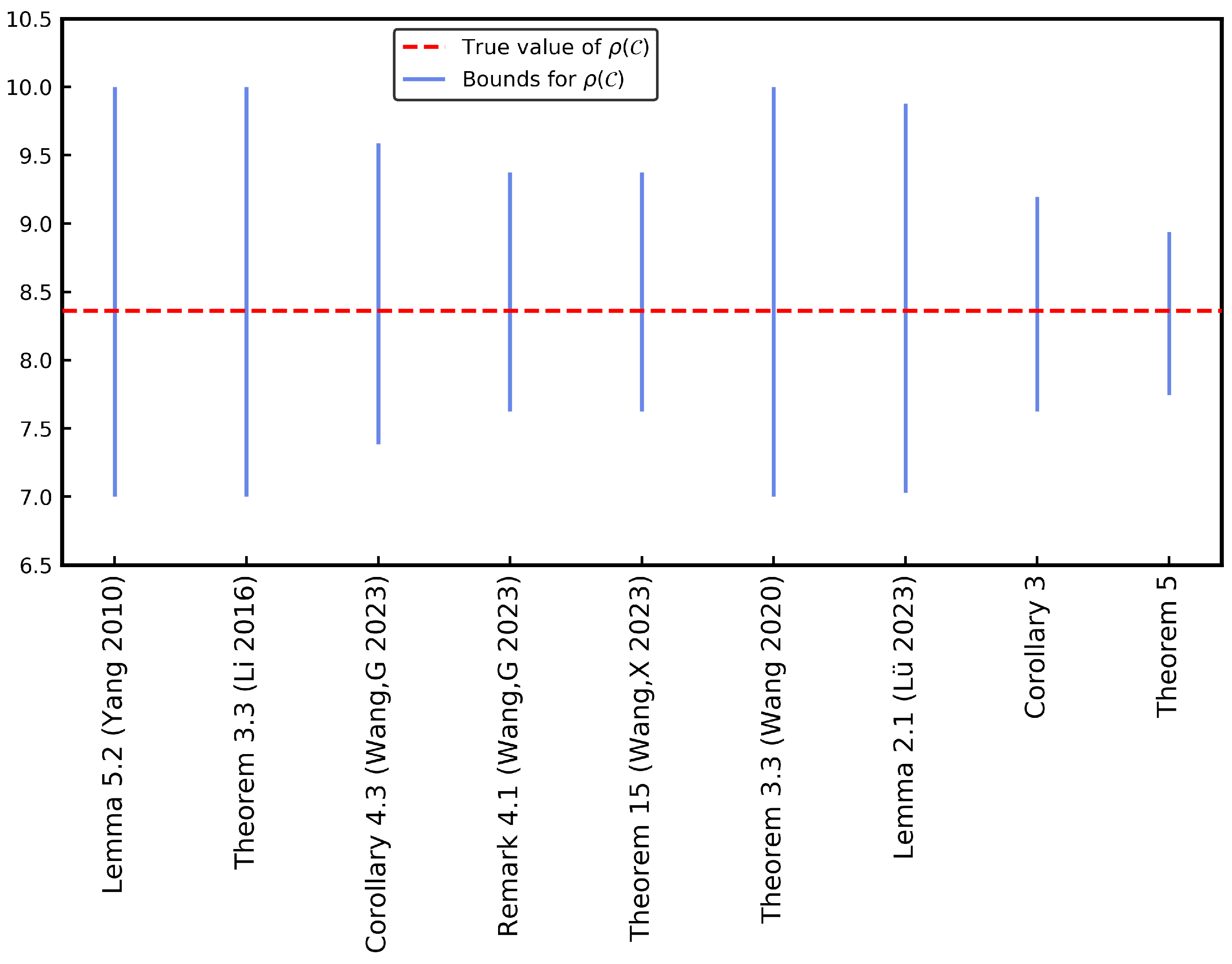
Let $S=\{1,4\}$; then $\overline{S}=\{2,3\}$. By calculations, the numerical comparisons among Corollary 3, Theorem 5 and the results in [5,8,12,14,16,20] are presented in Figure 1.

By analyzing the results in Figure 1, we can clearly observe that the bounds for $\rho \left(C\right)$ derived from our proposed Corollary 3 and Theorem 5 are both very close to the true value of $\rho \left(C\right)$, which demonstrates the effectiveness of our newly derived inequalities. More importantly, when compared with the existing bounds from [5,8,12,14,16,20], the intervals given by our results are significantly tighter. Moreover, the bound obtained by Theorem 5 is sharper than that in Corollary 3.

Figure 1. Numerical comparisons of the bounds for $\rho \left(\mathcal{C}\right)$ obtained by Lemma 5.2 in [12], Theorem 3.3 in [14], Corollary 4.3 and Remark 4.1 in [20], Theorem 15 in [5], Theorem 3.3 in [16], Lemma 2.1 in [8], Corollary 3 and Theorem 5.

Figure 1. Numerical comparisons of the bounds for $\rho \left(\mathcal{C}\right)$ obtained by Lemma 5.2 in [12], Theorem 3.3 in [14], Corollary 4.3 and Remark 4.1 in [20], Theorem 15 in [5], Theorem 3.3 in [16], Lemma 2.1 in [8], Corollary 3 and Theorem 5.

The above result demonstrates that the proposed inclusion sets are effective for deriving sharp inequalities related to the spectral radius of sparse tensors. Besides, eigenvalue inclusion sets can also be employed to study the positive definiteness of symmetric tensors. In the next section, we establish several criteria for checking the positive (semi-)definiteness of even-order symmetric sparse tensors.

5. Criteria for Positive (Semi-)Definiteness of Symmetric Sparse Tensors

In addition to spectral radius estimation, eigenvalue inclusion sets are also crucial for investigating the positive definiteness of symmetric tensors. Using the preceding results, we propose several criteria to assess the positive (semi-)definiteness of symmetric sparse tensors. The efficacy of our results is demonstrated through numerical examples.

Theorem 6.

Suppose $\mathcal{C}=\left(c_{i_1{i}_2\cdots i_m}\right)\in {\mathbb{R}}^{[m,n]}$ is even-order symmetric and $S\subseteq N$. For every $i\in N$, let $c_{ii\cdots i}>(\ge )0$. Assume that ${\mathsf{\Gamma }}_{M\left(\right|\mathcal{C}|)}^S\left(i\right)\ne \varnothing$ for every $i\in S$, ${\mathsf{\Gamma }}_{M\left(\right|\mathcal{C}|)}^{\overline{S}}\left(i\right)\ne \varnothing$ for every $i\in \overline{S}$. If

(i) 

$\left(c_{i\cdots i}-{\overline{r}}_i^S\left(\mathcal{C}\right)\right)c_{j\cdots j}>(\ge )r_j\left(\mathcal{C}\right){\tilde{r}}_i^S\left(\mathcal{C}\right)$, for any $(i,j)\in {\mathsf{\Lambda }}^S;$

(ii) 

$\left(c_{i\cdots i}-{\overline{r}}_i^{\overline{S}}\left(\mathcal{C}\right)\right)c_{j\cdots j}>(\ge )r_j\left(\mathcal{C}\right){\tilde{r}}_i^{\overline{S}}\left(\mathcal{C}\right)$, for any $(i,j)\in {\mathsf{\Lambda }}^{\overline{S}},$

then $\mathcal{C}$ is positive (semi-)definite.

Proof. 

We proceed to examine the condition of positive semi-definiteness. Similarly, we obtain the proof for the other case. Consider an $\mathrm{H}$-eigenvalue $\lambda$ of $\mathcal{C}$. We assume $\lambda$ is negative. In view of Theorem 1, it is evident that $\lambda \in {\tilde{\mathcal{T}}}^S\left(\mathcal{C}\right)$, which implies that there exists $(i_0,j_0)\in {\mathsf{\Lambda }}^S$ or $(i_0^{\prime },j_0^{\prime })\in {\mathsf{\Lambda }}^{\overline{S}}$ such that

$$\lambda \in {\mathcal{T}}_{i_0,j_0}^S\left(\mathcal{C}\right)\mathrm{or}\lambda \in {\mathcal{T}}_{i_0^{\prime },j_0^{\prime }}^{\overline{S}}\left(\mathcal{C}\right),$$

i.e.,

$$\left(|\lambda -c_{i_0\cdots i_0}|-{\overline{r}}_{i_0}^S\left(\mathcal{C}\right)\right)\left|\lambda -c_{j_0\cdots j_0}\right|\le r_{j_0}\left(\mathcal{C}\right){\tilde{r}}_{i_0}^S\left(\mathcal{C}\right)$$

or

$$\left(|\lambda -c_{i_0^{\prime }\cdots i_0^{\prime }}|-{\overline{r}}_{i_0^{\prime }}^{\overline{S}}\left(\mathcal{C}\right)\right)\left|\lambda -c_{j_0^{\prime }\cdots j_0^{\prime }}\right|\le r_{j_0^{\prime }}\left(\mathcal{C}\right){\tilde{r}}_{i_0^{\prime }}^{\overline{S}}\left(\mathcal{C}\right).$$

Since $\mathcal{C}$ satisfies the given condition with $c_{ii\cdots i}\ge 0$ for every $i\in N$, and $\lambda <0$, it is obvious that

$$\left(|\lambda -c_{i_0\cdots i_0}|-{\overline{r}}_{i_0}^S\left(\mathcal{C}\right)\right)\left|\lambda -c_{j_0\cdots j_0}\right|>\left(c_{i_0\cdots i_0}-{\overline{r}}_{i_0}^S\left(\mathcal{C}\right)\right)c_{j_0\cdots j_0}\ge r_{j_0}\left(\mathcal{C}\right){\tilde{r}}_{i_0}^S\left(\mathcal{C}\right)$$

and

$$\left(|\lambda -c_{i_0^{\prime }\cdots i_0^{\prime }}|-{\overline{r}}_{i_0^{\prime }}^{\overline{S}}\left(\mathcal{C}\right)\right)\left|\lambda -c_{j_0^{\prime }\cdots j_0^{\prime }}\right|>\left(c_{i_0^{\prime }\cdots i_0^{\prime }}-{\overline{r}}_{i_0^{\prime }}^{\overline{S}}\left(\mathcal{C}\right)\right)c_{j_0^{\prime }\cdots j_0^{\prime }}\ge r_{j_0^{\prime }}\left(\mathcal{C}\right){\tilde{r}}_{i_0^{\prime }}^{\overline{S}}\left(\mathcal{C}\right).$$

This yields a contradiction, which means that all $\mathrm{H}$-eigenvalues of $\mathcal{C}$ are nonnegative. Consequently, we obtain $\mathcal{C}$ is positive semi-definite. □

Adopting the proof strategy employed in Theorem 6, the conclusion is readily derived from Corollary 1.

Corollary 5.

Suppose $\mathcal{C}=\left(c_{i_1{i}_2\cdots i_m}\right)\in {\mathbb{R}}^{[m,n]}$ is even-order symmetric and $S\subseteq N$. For every $i\in N$, let $c_{ii\cdots i}>(\ge )0.$ If

(i) 

$\left(c_{i\cdots i}-{\overline{r}}_i^S\left(\mathcal{C}\right)\right)c_{j\cdots j}>(\ge )r_j\left(\mathcal{C}\right){\tilde{r}}_i^S\left(\mathcal{C}\right)$, $\mathit{for}\mathit{any}(i,j)\in {\mathsf{\Lambda }}^S\cup \{(i,j):i\in S,j=\underset{r\in \overline{S}}{max}r\}$;

(ii) 

$\left(c_{i\cdots i}-{\overline{r}}_i^{\overline{S}}\left(\mathcal{C}\right)\right)c_{j\cdots j}>(\ge )r_j\left(\mathcal{C}\right){\tilde{r}}_i^{\overline{S}}\left(\mathcal{C}\right)$, $\mathit{for}\mathit{any}(i,j)\in {\mathsf{\Lambda }}^{\overline{S}}\cup \{(i,j):i\in \overline{S},j=\underset{r\in S}{max}r\}$,

then $\mathcal{C}$ is positive (semi-)definite.

By employing arguments analogous to those presented in Theorem 6 and Corollary 5, we derive the following results, respectively.

Theorem 7.

Suppose $\mathcal{C}=\left(c_{i_1{i}_2\dots i_m}\right)\in {\mathbb{R}}^{[m,n]}$ is even-order symmetric and $S\subseteq N$. For arbitrary $i\in N$, let $c_{ii\cdots i}>(\ge )0.$ Assume that ${\mathsf{\Gamma }}_{G\left(\right|\mathcal{C}\left|\right)}^S\left(i\right)\ne \varnothing$ for every $i\in S$ and ${\mathsf{\Gamma }}_{G\left(\right|\mathcal{C}\left|\right)}^{\overline{S}}\left(i\right)\ne \varnothing$ for every $i\in \overline{S}$. If

(i) 

$\left(c_{i\cdots i}-r_i^{\overline{{\Delta }^{\overline{S}}}}\left(\mathcal{C}\right)\right)c_{j\cdots j}>(\ge )r_j\left(\mathcal{C}\right)r_i^{{\Delta }^{\overline{S}}}\left(\mathcal{C}\right)$, for any $(i,j)\in {\nabla }^S$;

(ii) 

$\left(c_{i\cdots i}-r_i^{\overline{{\Delta }^S}}\left(\mathcal{C}\right)\right)c_{j\cdots j}>(\ge )r_j\left(\mathcal{C}\right)r_i^{{\Delta }^S}\left(\mathcal{C}\right)$, for any $(i,j)\in {\nabla }^{\overline{S}}$,

then $\mathcal{C}$ is positive (semi-)definite.

Corollary 6.

Suppose $\mathcal{C}=\left(c_{i_1{i}_2\dots i_m}\right)\in {\mathbb{R}}^{[m,n]}$ is even-order symmetric and $S\subseteq N$. For every $i\in N$, let $c_{i\cdots i}>(\ge )0$. If

(i) 

$\left(c_{i\cdots i}-r_i^{\overline{{\Delta }^{\overline{S}}}}\left(\mathcal{C}\right)\right)c_{j\cdots j}>(\ge )r_j\left(\mathcal{C}\right)r_i^{{\Delta }^{\overline{S}}}\left(\mathcal{C}\right)$, $\mathit{for}\mathit{any}(i,j)\in {\nabla }^S\cup \{(i,j):i\in S,j=\underset{r\in \overline{S}}{max}r\}$;

(ii) 

$\left(c_{i\cdots i}-r_i^{\overline{{\Delta }^S}}\left(\mathcal{C}\right)\right)c_{j\cdots j}>(\ge )r_j\left(\mathcal{C}\right)r_i^{{\Delta }^S}\left(\mathcal{C}\right)$, $\mathit{for}\mathit{any}(i,j)\in {\nabla }^{\overline{S}}\cup \{(i,j):i\in \overline{S},j=\underset{r\in S}{max}r\}$,

then $\mathcal{C}$ is positive (semi-)definite.

The examples below serve to demonstrate the efficacy of our proposed criteria for checking the positive definiteness.

Example 2.

Let $\mathcal{C}=\left(c_{ijkl}\right)\in {\mathbb{R}}^{[4,4]}$, whose entries are given below:

$$\begin{array}{cc}\hfill & c_{1111}=2,c_{2222}=5,c_{3333}=9,c_{4444}=3,\hfill \\ \hfill & c_{1222}=-1,c_{2122}=-1,c_{2212}=-1,c_{2221}=-1,\hfill \\ \hfill & c_{1444}=-0.8,c_{4144}=-0.8,c_{4414}=-0.8,c_{4441}=-0.8,\hfill \\ \hfill & c_{4111}=-0.1,c_{1411}=-0.1,c_{1141}=-0.1,c_{1114}=-0.1,\hfill \\ \hfill & c_{3222}=-0.3,c_{2322}=-0.3,c_{2232}=-0.3,c_{2223}=-0.3,\hfill \\ \hfill & c_{2333}=-1.5,c_{3233}=-1.5,c_{3323}=-1.5,c_{3332}=-1.5.\hfill \end{array}$$

By applying the ZQW algorithm in [33], we further derive that the minimum $\mathrm{H}$-eigenvalue of $\mathcal{C}$ is $0.4246>0$. Hence, $\mathcal{C}$ is positive definite. Moreover, we have

$$G\left(\right|\mathcal{C}\left|\right)=\left(\begin{array}{cccc}2.3& 1& 0& 1.1\\ 3& 8.9& 2.4& 0\\ 0& 4.8& 13.5& 0\\ 2.5& 0& 0& 5.4\end{array}\right)\mathit{and}M\left(\right|\mathcal{C}|)=\left(\begin{array}{cccc}2& 1& 0& 0.8\\ 0& 5& 1.5& 0\\ 0& 0.3& 9& 0\\ 0.1& 0& 0& 3\end{array}\right).$$

From the definition of symmetric tensors, it is straightforward to check that $\mathcal{C}$ is symmetric. Let $S=\{1,2\}$; then $\overline{S}=\{3,4\}$. By Theorem 6, we can obtain the following table.

From Table 2, we can observe that for each pair $(i,j)$ listed in the table, the values in the second column are all strictly greater than the corresponding values in the third column. This indicates that all conditions stated in Theorem 6 are satisfied. Consequently, we can conclude that the tensor $\mathcal{C}$ is positive definite.

Table 2. Numerical results of Theorem 6.

$(\mathit{i},\mathit{j})$	$\left({\mathit{c}}_{\mathit{iiii}}-{\overline{\mathit{r}}}_{\mathit{i}}^{\mathit{S}}\left(\mathcal{C}\right)\right){\mathit{c}}_{\mathit{jjjj}}$ or $\left({\mathit{c}}_{\mathit{iiii}}-{\overline{\mathit{r}}}_{\mathit{i}}^{\overline{\mathit{S}}}\left(\mathcal{C}\right)\right){\mathit{c}}_{\mathit{jjjj}}$	${\tilde{\mathit{r}}}_{\mathit{i}}^{\mathit{S}}\left(\mathcal{C}\right){\mathit{r}}_{\mathit{j}}\left(\mathcal{C}\right)$ or ${\tilde{\mathit{r}}}_{\mathit{i}}^{\overline{\mathit{S}}}\left(\mathcal{C}\right){\mathit{r}}_{\mathit{j}}\left(\mathcal{C}\right)$
$(1,4)$	$2.10$	$2.00$
$(4,1)$	$1.20$	$0.21$
$(2,3)$	$9.90$	$7.20$
$(3,2)$	$22.5$	$1.62$

Choosing identical S, we can derive Table 3 from Theorem 7.

Table 3. Numerical results of Theorem 7.

$(\mathit{i},\mathit{j})$	$\left({\mathit{c}}_{\mathit{iiii}}-{\mathit{r}}_{\mathit{i}}^{\overline{{\mathbf{\Delta }}^{\mathit{S}}}}\left(\mathcal{C}\right)\right){\mathit{c}}_{\mathit{jjjj}}$ or $\left({\mathit{c}}_{\mathit{iiii}}-{\mathit{r}}_{\mathit{i}}^{\overline{{\Delta }^{\overline{\mathit{S}}}}}\left(\mathcal{C}\right)\right){\mathit{c}}_{\mathit{jjjj}}$	${\mathit{r}}_{\mathit{j}}\left(\mathcal{C}\right){\mathit{r}}_{\mathit{i}}^{{\Delta }^{\mathit{S}}}\left(\mathcal{C}\right)$ or ${\mathit{r}}_{\mathit{j}}\left(\mathcal{C}\right){\mathit{r}}_{\mathit{i}}^{{\Delta }^{\overline{\mathit{S}}}}\left(\mathcal{C}\right)$
$(1,4)$	$3.00$	$2.75$
$(4,1)$	$6.00$	$5.25$
$(2,3)$	$18.00$	$11.52$
$(3,2)$	$45.00$	$25.92$

From Table 3, we can also observe that for each pair $(i,j)$ listed in the table, the values in the second column are all strictly greater than the corresponding values in the third column. This indicates that all the inequalities required by Theorem 7 are strictly satisfied. Therefore, we can derive that the tensor $\mathcal{C}$ is positive definite.

By computation, we obtain

$$\left(c_{2222}-r_2^1\left(\mathcal{C}\right)\right)c_{1111}=-0.80<0.00=\left|c_{2111}\right|r_1\left(\mathcal{C}\right),$$

which does not satisfy the condition in Theorem 4.1 of [3]. Hence, Theorem 4.1 of [3] cannot be used to check whether $\mathcal{C}$ is positive definite. Similarly, Theorems 4.1 and 4.2 of [20] can not be applied to check whether $\mathcal{C}$ is positive definite.

Example 3.

Let $\mathcal{C}=\left(c_{ijkl}\right)\in {\mathbb{R}}^{[4,4]}$, whose entries are given below:

$$\begin{array}{cc}\hfill & c_{3333}=9,c_{1111}=2,c_{4444}=3,c_{2222}=4,\hfill \\ \hfill & c_{1222}=-1,c_{2122}=-1,c_{2212}=-1,c_{2221}=-1,\hfill \\ \hfill & c_{1444}=-0.8,c_{4144}=-0.8,c_{4414}=-0.8,c_{4441}=-0.8,\hfill \\ \hfill & c_{2333}=-1.5,c_{3233}=-1.5,c_{3323}=-1.5,c_{3332}=-1.5.\hfill \end{array}$$

By applying the ZQW algorithm, we further derive that the minimum $\mathrm{H}$-eigenvalue of $\mathcal{C}$ is $0.5097>0$. Hence, $\mathcal{C}$ is positive definite. Moreover, we have

$$G\left(\right|\mathcal{C}\left|\right)=\left(\begin{array}{cccc}2& 1& 0& 0.8\\ 3& 7& 1.5& 0\\ 0& 4.5& 13.5& 0\\ 2.4& 0& 0& 5.4\end{array}\right)\mathit{and}M\left(\right|\mathcal{C}|)=\left(\begin{array}{cccc}2& 1& 0& 0.8\\ 0& 4& 1.5& 0\\ 0& 0& 9& 0\\ 0& 0& 0& 3\end{array}\right).$$

From the definition of symmetric tensors, it is straightforward to check that $\mathcal{C}$ is symmetric. Let $S=\{1,2,4\}$; then $\overline{S}=\left\{3\right\}$. By Corollary 5, we can obtain the following table.

As illustrated in Table 4, which presents the numerical verification of Corollary 5, for all listed pairs, the values in the second column are strictly greater than the corresponding values in the third column. This indicates that all conditions of Corollary 5 are satisfied. Consequently, $\mathcal{C}$ is positive definite.

Table 4. Numerical results of Corollary 5.

$(\mathit{i},\mathit{j})$	$\left({\mathit{c}}_{\mathit{iiii}}-{\overline{\mathit{r}}}_{\mathit{i}}^{\mathit{S}}\left(\mathcal{C}\right)\right){\mathit{c}}_{\mathit{jjjj}}$ or $\left({\mathit{c}}_{\mathit{iiii}}-{\overline{\mathit{r}}}_{\mathit{i}}^{\overline{\mathit{S}}}\left(\mathcal{C}\right)\right){\mathit{c}}_{\mathit{jjjj}}$	${\tilde{\mathit{r}}}_{\mathit{i}}^{\mathit{S}}\left(\mathcal{C}\right){\mathit{r}}_{\mathit{j}}\left(\mathcal{C}\right)$ or  ${\tilde{\mathit{r}}}_{\mathit{i}}^{\overline{\mathit{S}}}\left(\mathcal{C}\right){\mathit{r}}_{\mathit{j}}\left(\mathcal{C}\right)$
$(3,4)$	$13.5$	$0.00$
$(1,3)$	$1.80$	$0.00$
$(4,3)$	$5.40$	$0.00$
$(2,3)$	$9.00$	$6.75$

Choosing identical S, we can derive Table 5 from Corollary 6.

Table 5. Numerical results of Corollary 6.

$(\mathit{i},\mathit{j})$	$\left({\mathit{c}}_{\mathit{iiii}}-{\mathit{r}}_{\mathit{i}}^{\overline{{\Delta }^{\mathit{S}}}}\left(\mathcal{C}\right)\right){\mathit{c}}_{\mathit{jjjj}}$ or $\left({\mathit{c}}_{\mathit{iiii}}-{\mathit{r}}_{\mathit{i}}^{\overline{{\Delta }^{\overline{\mathit{S}}}}}\left(\mathcal{C}\right)\right){\mathit{c}}_{\mathit{jjjj}}$	${\mathit{r}}_{\mathit{j}}\left(\mathcal{C}\right){\mathit{r}}_{\mathit{i}}^{{\Delta }^{\mathit{S}}}\left(\mathcal{C}\right)$ or ${\mathit{r}}_{\mathit{j}}\left(\mathcal{C}\right){\mathit{r}}_{\mathit{i}}^{{\Delta }^{\overline{\mathit{S}}}}\left(\mathcal{C}\right)$
$(3,4)$	$13.5$	$0.00$
$(1,3)$	$1.80$	$0.00$
$(2,3)$	$9.00$	$6.75$
$(4,3)$	$5.40$	$0.00$
$(3,2)$	$18.0$	$0.00$

For the results obtained from Corollary 6 shown in Table 5, we can similarly check that for all listed pairs, the values in the second column are strictly greater than those in the third. This means that all conditions of Corollary 6 are satisfied, and thus we can also confirm the positive definiteness of $\mathcal{C}$.

By applying a similar analysis as in Example 2, we find that Theorem 4.1 of [3], Corollaries 4.1 and 4.2 of [20] can not be applied to check whether $\mathcal{C}$ is positive definite.

6. Concluding Remarks

This study introduces two novel eigenvalue inclusion sets related to sparse tensors by employing the digraphs of the representation matrix and the majorization matrix. Based on these inclusion sets, we obtain new estimates for the spectral radius of weakly irreducible nonnegative sparse tensors and several criteria for verifying the positive (semi-)definiteness of even-order real symmetric sparse tensors. Additionally, numerical examples are provided to demonstrate the effectiveness of the proposed results. Selecting the proper subset S to minimize the bounds is an interesting yet practically challenging issue, especially for large-scale and high-dimensional sparse tensors. Therefore, in our future work, we will focus on designing adaptive or optimization-based strategies to choose a suitable subset S. This will further sharpen the eigenvalue localization sets and spectral radius bounds. Moreover, we will extend our results to structured tensors such as $\mathcal{M}$-tensors and $\mathcal{Z}$-tensors to explore their eigenvalue localization sets and related properties. Finally, we plan to explore the practical applications of the proposed inclusion sets and criteria, including hypergraph analysis, high-dimensional data processing and polynomial optimization.

References

- Qi, L. Eigenvalues of a real supersymmetric tensor. J. Symb. Comput. 2005, 40, 1302–1324. [Google Scholar] [CrossRef] [Scilit]
- Lim, L.H. Singular value and eigenvalue of tensors, a variational approach. In Proceedings of the 1st IEEE International Workshop on Computational Advances in Multi Sensor Adaptive Processing, Puerto Vallarta, Mexico, 13–15 December 2005; pp. 129–132. [Google Scholar]
- Li, C.; Li, Y.; Kong, X. New eigenvalue inclusion sets for tensors. Numer. Linear Algebr. Appl. 2014, 21, 39–50. [Google Scholar] [CrossRef] [Scilit]
- Zhang, Y.; Zhang, Y.; Wang, G. Exclusion sets in the S-type eigenvalue localization sets for tensors. Open Math. 2019, 17, 1136–1146. [Google Scholar] [CrossRef] [Scilit]
- Wang, X.; Lv, H. Quasi-Double Diagonally Dominant H-Tensors and the Estimation Inequalities for the Spectral Radius of Nonnegative Tensors. Symmetry 2023, 15, 439. [Google Scholar] [CrossRef] [Scilit]
- Li, C.; Jiao, A.; Li, Y. An S-type eigenvalue localization set for tensors. Linear Algebr. Appl. 2016, 493, 469–483. [Google Scholar] [CrossRef] [Scilit]
- Xu, Y. Brualdi-type inequalities on spectral radius for the Hadamard product of nonnegative tensors. Front. Math. 2025, 20, 87–108. [Google Scholar] [CrossRef] [Scilit]
- Lü, C.; You, L.; Huang, Y. Sharp Bounds for the Spectral Radii of Nonnegative Tensors. Front. Math. 2023, 18, 883–901. [Google Scholar] [CrossRef] [Scilit]
- Lv, H.; Chen, M. Linear convergence of the NQZ algorithm for finding the H-spectral radius of nonnegative tensors. PLoS ONE 2026, 21, e0338496. [Google Scholar] [CrossRef] [Scilit]
- Xu, Y.; Shao, L.Y.; He, G. On some spectral radius inequalities for the Hadamard product of nonnegative tensors. Bull. Malays. Math. Sci. Soc. 2024, 47, 10. [Google Scholar] [CrossRef] [Scilit]
- Liu, G.; Lv, H. Bounds for spectral radius of nonnegative tensors using matrix-digraph-based approach. J. Ind. Manag. Optim. 2023, 19, 105–116. [Google Scholar] [CrossRef] [Scilit]
- Yang, Y.; Yang, Q. Further results for Perron-Frobenius theorem for nonnegative tensors. SIAM J. Matrix Anal. Appl. 2010, 31, 2517–2530. [Google Scholar] [CrossRef] [Scilit]
- Yang, Y.; Yang, Q. On some properties of nonnegative weakly irreducible tensors. arXiv 2011, arXiv:1111.0713. [Google Scholar]
- Li, C.; Wang, Y.; Yi, J.; Li, Y. Bounds for the spectral radius of nonnegative tensor. J. Ind. Manag. Optim. 2016, 12, 975–990. [Google Scholar] [CrossRef] [Scilit]
- Sun, L.Z.; Zheng, B.D.; Zhou, J.; Yan, H. Some inequalities for the Hadamard product of tensors. Linear Multilinear Algebr. 2018, 66, 1199–1214. [Google Scholar] [CrossRef] [Scilit]
- Wang, G.; Wang, Y.; Wang, Y. Some Ostrowski-type bound estimations of spectral radius for weakly irreducible nonnegative tensors. Linear Multilinear Algebr. 2020, 68, 1817–1834. [Google Scholar] [CrossRef] [Scilit]
- Liu, P.; Liu, G.; Lv, H. Power Function Method for Finding the Spectral Radius of Weakly Irreducible Nonnegative Tensors. Symmetry 2022, 14, 2157. [Google Scholar] [CrossRef] [Scilit]
- Qi, L.; Luo, Z. Tensor Analysis: Spectral Theory and Special Tensors; SIAM: Philadelphia, PA, USA, 2017; pp. 261–268. [Google Scholar]
- Qi, L.; Cui, C.F. Biquadratic tensors: Eigenvalues and structured tensors. Symmetry 2025, 17, 1158. [Google Scholar] [CrossRef] [Scilit]
- Wang, G.; Feng, X. H-eigenvalue inclusion sets for sparse tensors. Bull. Malays. Math. Sci. Soc. 2023, 46, 164. [Google Scholar] [CrossRef] [Scilit]
- Feng, X.; Wang, G.; Wang, Y. New bounds of the minimum H-eigenvalue for sparse Z-tensors. Pac. J. Optim. 2025, 21, 179–194. [Google Scholar] [CrossRef] [Scilit]
- Cai, J.; Li, J.; Xia, D. Generalized Low-Rank Plus Sparse Tensor Estimation by Fast Riemannian Optimization. J. Am. Stat. Assoc. 2023, 118, 2588–2604. [Google Scholar] [CrossRef] [Scilit]
- Chang, J.; Chen, Y.; Qi, L. Computing eigenvalues of large scale sparse tensors arising from a hypergraph. SIAM J. Sci. Comput. 2016, 38, A3618–A3643. [Google Scholar] [CrossRef] [Scilit]
- Zeng, J.; Wang, C. Sparse tensor model-based spectral angle detector for hyperspectral target detection. IEEE Trans. Geosci. Remote Sens. 2022, 60, 1–15. [Google Scholar] [CrossRef] [Scilit]
- Zhang, X.; Ng, M. Sparse nonnegative tensor factorization and completion with noisy observations. IEEE Trans. Inf. Theory 2022, 68, 2551–2572. [Google Scholar] [CrossRef] [Scilit]
- Drikvandi, R.; Lawal, O. Sparse principal component analysis for natural language processing. Ann. Data Sci. 2023, 10, 25–41. [Google Scholar] [CrossRef] [Scilit]
- Yang, W.P.; Gao, H.X.; Zou, W.B.; Huang, S.S.; Chen, H.S.; Ma, J.L. Enhancing Low-Light Images: A Variation-based Retinex with Modified Bilateral Total Variation and Tensor Sparse Coding. Comput. Graph. Forum 2023, 42, e14960. [Google Scholar] [CrossRef] [Scilit]
- Zhang, Y.; Liu, Q.; Chen, Z. Preconditioned Jacobi type method for solving multi-linear systems with M-tensors. Appl. Math. Lett. 2020, 104, 106287. [Google Scholar] [CrossRef] [Scilit]
- Lv, H.; Chen, M. Algorithm and linear convergence of the H-spectral radius of weakly irreducible quasi-positive tensors. Open Math. 2025, 23, 20250194. [Google Scholar] [CrossRef] [Scilit]
- Friedland, S.; Gaubert, S.; Han, L. Perron-Frobenius theorems for nonnegative multilinear forms and extensions. Linear Algebr. Appl. 2013, 438, 738–749. [Google Scholar] [CrossRef] [Scilit]
- Pearson, K.J. Essentially positive tensors. Int. J. Algebr. 2010, 4, 421–427. [Google Scholar]
- Horn, R.A.; Johnson, C.R. Matrix Analysis, 2nd ed.; Cambridge University Press: Cambridge, UK, 2012. [Google Scholar]
- Zhou, G.; Qi, L.; Wu, S.Y. Efficient algorithms for computing the largest eigenvalue of a nonnegative tensor. Front. Math. China 2013, 8, 155–168. [Google Scholar] [CrossRef] [Scilit]
Disclaimer/Publisher’s Note: The statements, opinions and data contained in all publications are solely those of the individual author(s) and contributor(s) and not of MDPI and/or the editor(s). MDPI and/or the editor(s) disclaim responsibility for any injury to people or property resulting from any ideas, methods, instructions or products referred to in the content. |
© 2026 by the authors. Licensee MDPI, Basel, Switzerland. This article is an open access article distributed under the terms and conditions of the Creative Commons Attribution (CC BY) license.