Exploring Degenerate Peter–Genocchi Polynomials and Their Graphical Analysis

Abstract

In this paper, we introduce and investigate a new class of special polynomials called degenerate Peter–Genocchi polynomials. We define these polynomials and their associated numbers via an explicit generating function and explore a variety of their fundamental algebraic and analytic properties. In particular, we derive summation formulas (expressing polynomials via their associated numbers), addition formulas (splitting the polynomial argument), an implicit summation formula (a bivariate convolution identity), and symmetric identities. We also establish connections with degenerate Stirling numbers of both kinds, higher-order degenerate Genocchi polynomials, and higher-order degenerate Daehee polynomials. Furthermore, we investigate derivative properties and present a differential operator formula. Finally, we provide tables of approximate zeros and graphical representations of the zeros in the complex plane.

1. Introduction

Special polynomials and numbers occupy a central position in modern mathematics and its applications to physics, engineering, number theory, and combinatorics. Among the many families of special polynomials, Genocchi polynomials and numbers [1,2,3,4,5,6,7,8,9,10,11,12] have been extensively studied owing to their deep connections with p-adic analysis, quantum groups, stable homotopy theory, and differential topology. Concurrently, the Boole, Changhee, Daehee, and Peter polynomial families [13,14,15,16,17,18,19] have generated rich mathematical structures whose interactions with the Genocchi family continue to yield novel identities and relations.

A significant recent development is the introduction of Boole–Genocchi polynomials [13] and, subsequently, Peter–Genocchi polynomials [20] (also referred to as higher-order Boole–Genocchi polynomials). These polynomials combine the higher-order Boole (Peter) generating structure with the Genocchi generating kernel, producing a class with properties that generalize both families simultaneously.

In parallel with these developments, the study of degenerate versions of classical special polynomials and numbers has become a major theme in recent research. The degenerate approach, pioneered in the modern context by Carlitz [21] and subsequently extended by Kim and collaborators [22,23,24], replaces the classical exponential $e^{u\tau }$ by the degenerate exponential

$$e_{\lambda }^u\left(\tau \right):={(1+\lambda \tau )}^{u/\lambda },$$

(1)

which satisfies ${lim}_{\lambda \to 0}{(1+\lambda \tau )}^{u/\lambda }=e^{u\tau }$. The generating-function parameter is written as $\tau$ throughout, and auxiliary parameters appearing when two independent generating series are multiplied are denoted by $\upsilon$, $\varsigma$, etc.

Motivated by these developments, the present paper introduces the degenerate Peter–Genocchi polynomials $P{G}_{n,\lambda }(u;\alpha ,\mu )$. The paper is organized as follows. Section 2 introduces degenerate Peter–Genocchi polynomials and establishes their basic properties. Section 3 derives relations with degenerate Stirling numbers and other degenerate polynomial families. Section 4 investigates derivative properties and a differential operator formula. Section 5 presents the first few members, tables of approximate zeros, and graphical representations. Section 6 contains our concluding remarks.

We use $\tau$ for the formal generating-function parameter; polynomial variables are u, v, w, z; and $\upsilon$, $\varsigma$ denote auxiliary parameters. Throughout, ${\mathbb{N}}_0=\{0,1,2,\dots \}$ denotes the set of non-negative integers and $\mathbb{N}=\{1,2,3,\dots \}$ the set of positive integers.

Terminology. We will briefly outline the key terms used throughout the paper. A generating function (or generating series) for a sequence ${\left\{a_n\right\}}_{n\ge 0}$ is the formal power series ${\sum }_{n=0}^{\infty }{a}_n{\tau }^n/n!$. A degenerate Taylor expansion refers to expanding a function in terms of the degenerate falling factorials ${\left(u\right)}_{n,\lambda }$ rather than ordinary powers $u^n$; see (2). By a zero (or root) of a polynomial $p\left(u\right)$, we mean a value $u\in \mathbb{C}$ satisfying $p\left(u\right)=0$. The phrase zero evolution describes how the zeros of $P{G}_{n,\lambda }(u;\alpha ,\mu )$ in the complex plane change as the degree n increases.

Background definitions.

The degenerate exponential function is defined, for $\lambda \in \mathbb{R}$, by

$$e_{\lambda }^u\left(\tau \right)={(1+\lambda \tau )}^{u/\lambda }={\displaystyle \sum _{n=0}^{\infty }}{\left(u\right)}_{n,\lambda }{\displaystyle \frac{{\tau }^n}{n!}},$$

(2)

where the degenerate falling factorial ${\left(u\right)}_{n,\lambda }$ is

$${\left(u\right)}_{0,\lambda }=1,{\left(u\right)}_{n,\lambda }=u(u-\lambda )(u-2\lambda )\dots \left(u-(n-1)\lambda \right)(n\ge 1).$$

(3)

Note that ${lim}_{\lambda \to 0}{\left(u\right)}_{n,\lambda }=u^n$ and ${lim}_{\lambda \to 0}{e}_{\lambda }^u\left(\tau \right)=e^{u\tau }$.

The degenerate logarithm is defined by

$${log}_{\lambda }(1+\tau )={\displaystyle \frac{{(1+\tau )}^{\lambda }-1}{\lambda }},\underset{\lambda \to 0}{lim}{log}_{\lambda }(1+\tau )=log(1+\tau ).$$

(4)

It is the compositional inverse of $e_{\lambda }^1\left(\tau \right)-1={(1+\lambda \tau )}^{1/\lambda }-1$: that is, ${log}_{\lambda }(e_{\lambda }^1\left(\tau \right)-1+1)=\tau$ and $e_{\lambda }^1({log}_{\lambda }(1+\tau )-1+1)=1+\tau$.

Remark 1.

It is important to note that ${log}_{\lambda }(1+\tau )\ne log(1+\tau )$ for $\lambda \ne 0$. Here and throughout, limits as $\lambda \to 0$ are understood in the sense of formal power series (i.e., coefficient-wise). All proofs below use ${log}_{\lambda }$ consistently and do not substitute the classical logarithm in its place.

The higher-order degenerate Genocchi polynomials $G_{n,\lambda }^{\left(\mu \right)}\left(u\right)$, for $\mu \in \mathbb{R}$, are given by (cf. [4,22])

$${\displaystyle \sum _{n=0}^{\infty }}{G}_{n,\lambda }^{\left(\mu \right)}\left(u\right){\displaystyle \frac{{\tau }^n}{n!}}={(1+\lambda \tau )}^{u/\lambda }{\left({\displaystyle \frac{2{log}_{\lambda }(1+\tau )}{{(1+\lambda \tau )}^{1/\lambda }+1}}\right)}^{\mu }.$$

(5)

Setting $u=0$ gives $G_{n,\lambda }^{\left(\mu \right)}:=G_{n,\lambda }^{\left(\mu \right)}\left(0\right)$.

The higher-order degenerate Changhee polynomials $C{H}_{n,\lambda }^{\left(\mu \right)}\left(u\right)$, for $\mu \in \mathbb{R}$, are given by (cf. [3])

$${\displaystyle \sum _{n=0}^{\infty }}C{H}_{n,\lambda }^{\left(\mu \right)}\left(u\right){\displaystyle \frac{{\tau }^n}{n!}}={\left({\displaystyle \frac{2}{2+\tau }}\right)}^{\mu }{(1+\tau )}^u.$$

(6)

The higher-order degenerate Daehee polynomials $D_{n,\lambda }^{\left(\mu \right)}\left(u\right)$, for $\mu \in \mathbb{R}$, are given by (cf. [25])

$${\displaystyle \sum _{n=0}^{\infty }}{D}_{n,\lambda }^{\left(\mu \right)}\left(u\right){\displaystyle \frac{{\tau }^n}{n!}}={(1+\tau )}^u{\left({\displaystyle \frac{{log}_{\lambda }(1+\tau )}{\tau }}\right)}^{\mu }.$$

(7)

The degenerate Stirling numbers $S_{1,\lambda }(n,k)$ and $S_{2,\lambda }(n,k)$ are given, for $k\in {\mathbb{N}}_0$, by (cf. [23,24,26])

$${\displaystyle \frac{{\left({log}_{\lambda }(1+\tau )\right)}^k}{k!}}={\displaystyle \sum _{n=0}^{\infty }}{S}_{1,\lambda }(n,k){\displaystyle \frac{{\tau }^n}{n!}},{\displaystyle \frac{{\left(e_{\lambda }^1\left(\tau \right)-1\right)}^k}{k!}}={\displaystyle \sum _{n=0}^{\infty }}{S}_{2,\lambda }(n,k){\displaystyle \frac{{\tau }^n}{n!}}.$$

(8)

As $\lambda \to 0$ these reduce to the classical Stirling numbers. The key identity relating falling factorials to powers is

$${\left(v\right)}_{j,\lambda }={\displaystyle \sum _{k=0}^j}{S}_{1,\lambda }(j,k)v^k,\mathrm{so}\mathrm{that}{(1+\lambda \tau )}^{v/\lambda }={\displaystyle \sum _{j=0}^{\infty }}\left({\displaystyle \sum _{k=0}^j}{S}_{1,\lambda }(j,k)v^k\right){\displaystyle \frac{{\tau }^j}{j!}}.$$

(9)

The higher-order Peter polynomials $s_n(u;\alpha ,\mu )$, for $\alpha ,\mu \in \mathbb{R}$, are given by (cf. [17,19])

$${\displaystyle \frac{{(1+\tau )}^u}{{\left(1+{(1+\tau )}^{\alpha }\right)}^{\mu }}}={\displaystyle \sum _{n=0}^{\infty }}{s}_n(u;\alpha ,\mu ){\displaystyle \frac{{\tau }^n}{n!}}.$$

(10)

The Peter–Genocchi polynomials $P{G}_n(u;\alpha ,\mu )$ [20] are generated by

$${\displaystyle \frac{{\left(log(1+\tau )\right)}^{\mu }}{{\left(1+{(1+\tau )}^{\alpha }\right)}^{\mu }}}{(1+\tau )}^u={\displaystyle \sum _{n=0}^{\infty }}P{G}_n(u;\alpha ,\mu ){\displaystyle \frac{{\tau }^n}{n!}}.$$

(11)

2. Degenerate Peter–Genocchi Polynomials: Definition and Basic Properties

The remarks in this section highlight important special cases of the degenerate Peter–Genocchi polynomials, showing how they reduce to known polynomial families (Boole–Genocchi and Changhee–Genocchi) under particular parameter choices.

Definition 1. 

Let $\alpha ,\mu ,\lambda \in \mathbb{R}$. The degenerate Peter–Genocchi polynomials $P{G}_{n,\lambda }(u;\alpha ,\mu )$ are defined by

$${\displaystyle \frac{{\left({log}_{\lambda }(1+\tau )\right)}^{\mu }}{{\left(1+{(1+\tau )}^{\alpha }\right)}^{\mu }}}{(1+\lambda \tau )}^{u/\lambda }={\displaystyle \sum _{n=0}^{\infty }}P{G}_{n,\lambda }(u;\alpha ,\mu ){\displaystyle \frac{{\tau }^n}{n!}}.$$

(12)

Setting $u=0$ yields the degenerate Peter–Genocchi numbers $P{G}_{n,\lambda }(\alpha ,\mu ):=P{G}_{n,\lambda }(0;\alpha ,\mu )$, whose generating series is

$${\displaystyle \frac{{\left({log}_{\lambda }(1+\tau )\right)}^{\mu }}{{\left(1+{(1+\tau )}^{\alpha }\right)}^{\mu }}}={\displaystyle \sum _{n=0}^{\infty }}P{G}_{n,\lambda }(\alpha ,\mu ){\displaystyle \frac{{\tau }^n}{n!}}.$$

(13)

Remark 2.

As $\lambda \to 0$, ${(1+\lambda \tau )}^{u/\lambda }\to e^{u\tau }$ and ${log}_{\lambda }(1+\tau )\to log(1+\tau )$, so (12) reduces to (11).

Remark 3.

Setting $\mu =1$ in (12) yields the degenerate Boole–Genocchi polynomials $B{G}_{n,\lambda }(u;\alpha )$:

$${\displaystyle \frac{{log}_{\lambda }(1+\tau )}{1+{(1+\tau )}^{\alpha }}}{(1+\lambda \tau )}^{u/\lambda }={\displaystyle \sum _{n=0}^{\infty }}B{G}_{n,\lambda }(u;\alpha ){\displaystyle \frac{{\tau }^n}{n!}}.$$

Remark 4.

Setting $\alpha =1$ in (12) produces higher-order degenerate Changhee–Genocchi polynomials:

$${\displaystyle \frac{2^{\mu }{\left({log}_{\lambda }(1+\tau )\right)}^{\mu }}{{(2+\tau )}^{\mu }}}{(1+\lambda \tau )}^{u/\lambda }={\displaystyle \sum _{n=0}^{\infty }}C{G}_{n,\lambda }^{\left(\mu \right)}\left(u\right){\displaystyle \frac{{\tau }^n}{n!}}.$$

Remark 5.

Setting $\mu =\alpha =1$ yields degenerate Changhee–Genocchi polynomials:

$${\displaystyle \frac{2{log}_{\lambda }(1+\tau )}{2+\tau }}{(1+\lambda \tau )}^{u/\lambda }={\displaystyle \sum _{n=0}^{\infty }}C{G}_{n,\lambda }\left(u\right){\displaystyle \frac{{\tau }^n}{n!}}.$$

Theorem 1.

For $n\in {\mathbb{N}}_0$ and $\alpha ,\mu \in \mathbb{R}$,

$$P{G}_{n,\lambda }(u;\alpha ,\mu )={\displaystyle \sum _{k=0}^n}\left({\displaystyle \genfrac{}{}{0pt}{}{n}{k}}\right)P{G}_{n-k,\lambda }(\alpha ,\mu ){\left(u\right)}_{k,\lambda }.$$

(14)

Proof. 

From (2), ${(1+\lambda \tau )}^{u/\lambda }={\sum }_{k=0}^{\infty }{\left(u\right)}_{k,\lambda }{\displaystyle \frac{{\tau }^k}{k!}}$. Multiplying by the generating series (13) and applying the Cauchy product formula (see, e.g., [27])

$$\begin{array}{cc}\hfill {\displaystyle \sum _{n=0}^{\infty }}P{G}_{n,\lambda }(u;\alpha ,\mu ){\displaystyle \frac{{\tau }^n}{n!}}& =\left({\displaystyle \sum _{n=0}^{\infty }}P{G}_{n,\lambda }(\alpha ,\mu ){\displaystyle \frac{{\tau }^n}{n!}}\right)\left({\displaystyle \sum _{k=0}^{\infty }}{\left(u\right)}_{k,\lambda }{\displaystyle \frac{{\tau }^k}{k!}}\right)\hfill \\ \hfill & ={\displaystyle \sum _{n=0}^{\infty }}\left({\displaystyle \sum _{k=0}^n}{\displaystyle \frac{P{G}_{n-k,\lambda }(\alpha ,\mu )}{(n-k)!}}·{\displaystyle \frac{{\left(u\right)}_{k,\lambda }}{k!}}\right){\tau }^n\hfill \\ \hfill & ={\displaystyle \sum _{n=0}^{\infty }}\left({\displaystyle \sum _{k=0}^n}\left({\displaystyle \genfrac{}{}{0pt}{}{n}{k}}\right)P{G}_{n-k,\lambda }(\alpha ,\mu ){\left(u\right)}_{k,\lambda }\right){\displaystyle \frac{{\tau }^n}{n!}},\hfill \end{array}$$

where we used ${\displaystyle \frac{1}{(n-k)!k!}}={\displaystyle \frac{1}{n!}}\left({\displaystyle \genfrac{}{}{0pt}{}{n}{k}}\right)$. Comparing coefficients of ${\displaystyle \frac{{\tau }^n}{n!}}$ yields (14).    □

Theorem 2. 

For $n\in {\mathbb{N}}_0$ and $\alpha ,\mu \in \mathbb{R}$,

$$P{G}_{n,\lambda }(u+v;\alpha ,\mu )={\displaystyle \sum _{j=0}^n}{\displaystyle \sum _{k=0}^j}\left({\displaystyle \genfrac{}{}{0pt}{}{n}{j}}\right)P{G}_{n-j,\lambda }(u;\alpha ,\mu )S_{1,\lambda }(j,k)v^k$$

(15)

 and

$$P{G}_{n,\lambda }(u+v;\alpha ,\mu )={\displaystyle \sum _{j=0}^n}{\displaystyle \sum _{k=0}^j}\left({\displaystyle \genfrac{}{}{0pt}{}{n}{j}}\right)P{G}_{n-j,\lambda }(\alpha ,\mu )S_{1,\lambda }(j,k){(u+v)}^k.$$

(16)

Proof of (15). 

Replace u by $u+v$ in (12) and use the multiplicative property ${(1+\lambda \tau )}^{(u+v)/\lambda }={(1+\lambda \tau )}^{u/\lambda }{(1+\lambda \tau )}^{v/\lambda }$. Hence

$${\displaystyle \sum _{n=0}^{\infty }}P{G}_{n,\lambda }(u+v;\alpha ,\mu ){\displaystyle \frac{{\tau }^n}{n!}}=\left({\displaystyle \sum _{n=0}^{\infty }}P{G}_{n,\lambda }(u;\alpha ,\mu ){\displaystyle \frac{{\tau }^n}{n!}}\right){(1+\lambda \tau )}^{v/\lambda }.$$

By (9), ${(1+\lambda \tau )}^{v/\lambda }={\sum }_{j=0}^{\infty }\left({\sum }_{k=0}^j{S}_{1,\lambda }(j,k)v^k\right){\displaystyle \frac{{\tau }^j}{j!}}$. Applying the Cauchy product and comparing the coefficients of ${\displaystyle \frac{{\tau }^n}{n!}}$ yields (15).    □

Proof of (16). 

Write the generating Function (12) at argument $u+v$ as $\left(\mathrm{numbers}\mathrm{generating}\mathrm{series}\right)$$\times {(1+\lambda \tau )}^{(u+v)/\lambda }$. By (9) with v replaced by $u+v$, ${(1+\lambda \tau )}^{(u+v)/\lambda }={\sum }_j\left({\sum }_k{S}_{1,\lambda }(j,k){\left(u+v\right)}^k\right){\displaystyle \frac{{\tau }^j}{j!}}$. Applying the Cauchy product with (13) and comparing coefficients results in (16).    □

Remark 6.  

Three special cases of Theorem 2: setting $v=0$ in (15), $P{G}_{n,\lambda }(u;\alpha ,\mu )={\sum }_{j,k}\left({\displaystyle \genfrac{}{}{0pt}{}{n}{j}}\right)P{G}_{n-j,\lambda }(\alpha ,\mu )S_{1,\lambda }(j,k)u^k$ (this is consistent with Theorem 1 via the identity ${\left(u\right)}_{j,\lambda }={\sum }_k{S}_{1,\lambda }(j,k)u^k$); setting $u=0$, $P{G}_{n,\lambda }(v;\alpha ,\mu )={\sum }_{j,k}\left({\displaystyle \genfrac{}{}{0pt}{}{n}{j}}\right)P{G}_{n-j,\lambda }(\alpha ,\mu )S_{1,\lambda }(j,k)v^k$; setting $v=1$, $P{G}_{n,\lambda }(u+1;\alpha ,\mu )={\sum }_{j,k}\left({\displaystyle \genfrac{}{}{0pt}{}{n}{j}}\right)P{G}_{n-j,\lambda }(u;\alpha ,\mu )S_{1,\lambda }(j,k)$.

Theorem 3. 

For $k,l\in {\mathbb{N}}_0$, $\alpha ,\mu \in \mathbb{R}$, and any $w\in \mathbb{R}$,

$$P{G}_{k+l,\lambda }(u;\alpha ,\mu )={\displaystyle \sum _{n=0}^k}{\displaystyle \sum _{m=0}^l}\left({\displaystyle \genfrac{}{}{0pt}{}{k}{n}}\right)\left({\displaystyle \genfrac{}{}{0pt}{}{l}{m}}\right)P{G}_{k+l-n-m,\lambda }(w;\alpha ,\mu ){(u-w)}_{n+m,\lambda }.$$

(17)

Proof. 

 

Step 1. Replace $\tau$ by $\tau +\upsilon$ in (12) with argument w and apply the series identity ${\sum }_{k,l\ge 0}f(k+l){\displaystyle \frac{{\tau }^k}{k!}}{\displaystyle \frac{{\upsilon }^l}{l!}}={\sum }_{n\ge 0}f\left(n\right){\displaystyle \frac{{(\tau +\upsilon )}^n}{n!}}$ (cf. [13,20]) with $f\left(n\right)=P{G}_{n,\lambda }(w;\alpha ,\mu )$:

$${\displaystyle \frac{{\left({log}_{\lambda }(1+\tau +\upsilon )\right)}^{\mu }}{{\left(1+{(1+\tau +\upsilon )}^{\alpha }\right)}^{\mu }}}{(1+\lambda (\tau +\upsilon ))}^{w/\lambda }={\displaystyle \sum _{k,l=0}^{\infty }}P{G}_{k+l,\lambda }(w;\alpha ,\mu ){\displaystyle \frac{{\tau }^k}{k!}}{\displaystyle \frac{{\upsilon }^l}{l!}}.$$

(18)

Step 2. Multiply both sides of (18) by ${(1+\lambda (\tau +\upsilon ))}^{(u-w)/\lambda }$. The left-hand side then equals the generating Function (12) at argument u (after the same $\tau \mapsto \tau +\upsilon$ shift), giving

$${\displaystyle \sum _{k,l=0}^{\infty }}P{G}_{k+l,\lambda }(u;\alpha ,\mu ){\displaystyle \frac{{\tau }^k}{k!}}{\displaystyle \frac{{\upsilon }^l}{l!}}=\left({\displaystyle \sum _{k,l=0}^{\infty }}P{G}_{k+l,\lambda }(w;\alpha ,\mu ){\displaystyle \frac{{\tau }^k}{k!}}{\displaystyle \frac{{\upsilon }^l}{l!}}\right)·{(1+\lambda (\tau +\upsilon ))}^{(u-w)/\lambda }.$$

(19)

Step 3. We expand ${(1+\lambda (\tau +\upsilon ))}^{(u-w)/\lambda }$ exactly using (2):

$$\begin{array}{cc}\hfill {(1+\lambda (\tau +\upsilon ))}^{(u-w)/\lambda }& =e_{\lambda }^{u-w}(\tau +\upsilon )={\displaystyle \sum _{s=0}^{\infty }}{(u-w)}_{s,\lambda }{\displaystyle \frac{{(\tau +\upsilon )}^s}{s!}}\hfill \\ \hfill & ={\displaystyle \sum _{s=0}^{\infty }}{(u-w)}_{s,\lambda }\sum _{\begin{array}{c}n,m\ge 0\\ n+m=s\end{array}}{\displaystyle \frac{{\tau }^n}{n!}}{\displaystyle \frac{{\upsilon }^m}{m!}}={\displaystyle \sum _{n,m=0}^{\infty }}{(u-w)}_{n+m,\lambda }{\displaystyle \frac{{\tau }^n}{n!}}{\displaystyle \frac{{\upsilon }^m}{m!}}.\hfill \end{array}$$

(20)

Note carefully, the degenerate falling factorial ${(u-w)}_{n+m,\lambda }$ appears here, not the ordinary power ${(u-w)}^{n+m}$, because we use the exact degenerate Taylor expansion.

Step 4. Substitute (20) into the right-hand side of (19) and apply the Cauchy product for double power series. The coefficient of ${\displaystyle \frac{{\tau }^k}{k!}}{\displaystyle \frac{{\upsilon }^l}{l!}}$ on the right-hand side is

$${\displaystyle \sum _{n=0}^k}{\displaystyle \sum _{m=0}^l}\left({\displaystyle \genfrac{}{}{0pt}{}{k}{n}}\right)\left({\displaystyle \genfrac{}{}{0pt}{}{l}{m}}\right)P{G}_{k+l-n-m,\lambda }(w;\alpha ,\mu ){(u-w)}_{n+m,\lambda }.$$

Equating with the same coefficient on the left-hand side of (19) produces (17).    □

Remark 7. 

Two special cases of (17): setting $k=0$, $P{G}_{l,\lambda }(u;\alpha ,\mu )={\sum }_{m=0}^l\left({\displaystyle \genfrac{}{}{0pt}{}{l}{m}}\right)P{G}_{l-m,\lambda }(w;\alpha ,\mu ){(u-w)}_{m,\lambda }$; setting $w=0$, $P{G}_{l,\lambda }(u;\alpha ,\mu )={\sum }_{m=0}^l\left({\displaystyle \genfrac{}{}{0pt}{}{l}{m}}\right)P{G}_{l-m,\lambda }(0;\alpha ,\mu ){\left(u\right)}_{m,\lambda }$.

Theorem 4. 

For $n\in {\mathbb{N}}_0$ and $a,b,\alpha ,\beta ,\mu ,\nu \in \mathbb{R}$,

$$\begin{array}{c}{\displaystyle \sum _{k=0}^n}\left({\displaystyle \genfrac{}{}{0pt}{}{n}{k}}\right)P{G}_{n-k,\lambda }(u_1;\alpha ,\mu )P{G}_{k,\lambda }(u_2;\beta ,\nu )a^{n-k}{b}^k\hspace{1em}\hspace{1em}\hspace{1em}\hspace{1em}\hspace{1em}\hspace{1em}\hspace{1em}\hspace{1em}\hspace{1em}\hspace{1em}\hspace{1em}\hspace{1em}\hfill \\ \hfill \hspace{1em}\hspace{1em}\hspace{1em}\hspace{1em}\hspace{1em}\hspace{1em}\hspace{1em}\hspace{1em}\hspace{1em}\hspace{1em}\hspace{1em}\hspace{1em}={\displaystyle \sum _{k=0}^n}\left({\displaystyle \genfrac{}{}{0pt}{}{n}{k}}\right)P{G}_{n-k,\lambda }(u_2;\beta ,\nu )P{G}_{k,\lambda }(u_1;\alpha ,\mu )a^k{b}^{n-k}.\end{array}$$

(21)

Proof. 

Define

$${\rm Y}\left(\tau \right):={\displaystyle \frac{{\left({log}_{\lambda }(1+a\tau )\right)}^{\mu }{\left({log}_{\lambda }(1+b\tau )\right)}^{\nu }}{{\left(1+{(1+a\tau )}^{\alpha }\right)}^{\mu }{\left(1+{(1+b\tau )}^{\beta }\right)}^{\nu }}}{(1+\lambda a\tau )}^{u_1/\lambda }{(1+\lambda b\tau )}^{u_2/\lambda }.$$

Applying (12) with $\tau \mapsto a\tau$ yields ${\sum }_{n\ge 0}P{G}_{n,\lambda }(u_1;\alpha ,\mu )a^n{\displaystyle \frac{{\tau }^n}{n!}}$ for the first factors, and similarly for the b-group. Hence

$${\rm Y}\left(\tau \right)=\left({\displaystyle \sum _{n=0}^{\infty }}P{G}_{n,\lambda }(u_1;\alpha ,\mu )a^n{\displaystyle \frac{{\tau }^n}{n!}}\right)\left({\displaystyle \sum _{k=0}^{\infty }}P{G}_{k,\lambda }(u_2;\beta ,\nu )b^k{\displaystyle \frac{{\tau }^k}{k!}}\right),$$

and the Cauchy product yields $[{\tau }^n/n!]{\rm Y}={\sum }_{k=0}^n\left({\displaystyle \genfrac{}{}{0pt}{}{n}{k}}\right)P{G}_{n-k,\lambda }(u_1;\alpha ,\mu )P{G}_{k,\lambda }(u_2;\beta ,\nu )a^{n-k}{b}^k$. Since ${\rm Y}$ is symmetric under $(a,u_1,\alpha ,\mu )\leftrightarrow (b,u_2,\beta ,\nu )$, the same coefficient also equals ${\sum }_{k=0}^n\left({\displaystyle \genfrac{}{}{0pt}{}{n}{k}}\right)P{G}_{n-k,\lambda }(u_2;\beta ,\nu )P{G}_{k,\lambda }(u_1;\alpha ,\mu )a^k{b}^{n-k}$. Equating the two produces (21).    □

Theorem 5. 

For $n\in {\mathbb{N}}_0$ and $a,b,\alpha ,\mu \in \mathbb{R}$,

$$\begin{array}{c}{\displaystyle \sum _{l=0}^n}{\displaystyle \sum _{k=0}^{n-l}}{\displaystyle \sum _{s=0}^l}\left({\displaystyle \genfrac{}{}{0pt}{}{n}{l}}\right)\left({\displaystyle \genfrac{}{}{0pt}{}{n-l}{k}}\right)\left({\displaystyle \genfrac{}{}{0pt}{}{l}{s}}\right)P{G}_{n-l-k,\lambda }(\alpha ,\mu )P{G}_{l-s,\lambda }(\alpha ,\mu ){\left(u\right)}_{k,\lambda }{\left(u\right)}_{s,\lambda }{a}^{n+s-l}{b}^{l+k}\hfill \\ \hfill ={\displaystyle \sum _{l=0}^n}{\displaystyle \sum _{k=0}^l}{\displaystyle \sum _{s=0}^{n-l}}\left({\displaystyle \genfrac{}{}{0pt}{}{n}{l}}\right)\left({\displaystyle \genfrac{}{}{0pt}{}{l}{k}}\right)\left({\displaystyle \genfrac{}{}{0pt}{}{n-l}{s}}\right)P{G}_{l-k,\lambda }(\alpha ,\mu )P{G}_{n-l-s,\lambda }(\alpha ,\mu ){\left(u\right)}_{k,\lambda }{\left(u\right)}_{s,\lambda }{a}^{l+k}{b}^{n-l+s}.\end{array}$$

(22)

Proof. 

Define

$$\Psi \left(\tau \right):={\displaystyle \frac{{\left({log}_{\lambda }(1+a\tau )\right)}^{\mu }{\left({log}_{\lambda }(1+b\tau )\right)}^{\mu }}{{\left(1+{(1+a\tau )}^{\alpha }\right)}^{\mu }{\left(1+{(1+b\tau )}^{\alpha }\right)}^{\mu }}}{(1+\lambda ab\tau )}^{2u/\lambda }.$$

Since ${(1+\lambda ab\tau )}^{2u/\lambda }={(1+\lambda a\tau )}^{u/\lambda }{(1+\lambda b\tau )}^{u/\lambda }$, by Theorem 1 (with $\tau \mapsto a\tau$ and u replaced by the degenerate expansion),

$$\begin{array}{cc}\hfill {\displaystyle \frac{{\left({log}_{\lambda }(1+a\tau )\right)}^{\mu }}{{(1+{(1+a\tau )}^{\alpha })}^{\mu }}}{(1+\lambda a\tau )}^{u/\lambda }& ={\displaystyle \sum _{n=0}^{\infty }}\left({\displaystyle \sum _{k=0}^n}\left({\displaystyle \genfrac{}{}{0pt}{}{n}{k}}\right)P{G}_{n-k,\lambda }(\alpha ,\mu ){\left(u\right)}_{k,\lambda }{b}^k\right)a^n{\displaystyle \frac{{\tau }^n}{n!}},\hfill \end{array}$$

and analogously for the b-group (with $a^s$ inserted). Multiplying and applying the Cauchy product gives the left-hand side of (22) as the coefficient of ${\displaystyle \frac{{\tau }^n}{n!}}$. The right-hand side follows by swapping $a\leftrightarrow b$. Since $\Psi$ is symmetric under $a\leftrightarrow b$, equating the two expressions proves (22).    □

3. Relations with Degenerate Polynomial Families

Theorem 6. 

For $n,\mu \in {\mathbb{N}}_0$ and $\alpha \in \mathbb{R}$,

$$S_{1,\lambda }(n,\mu )={\displaystyle \frac{1}{\mu !}}{\displaystyle \sum _{m=0}^n}{\displaystyle \sum _{k=0}^{\mu }}\left({\displaystyle \genfrac{}{}{0pt}{}{n}{m}}\right)\left({\displaystyle \genfrac{}{}{0pt}{}{\mu }{k}}\right)P{G}_{n-m,\lambda }(u;\alpha ,\mu ){(k\alpha -u)}_{m,\lambda }.$$

(23)

Proof. 

Starting from (12), multiply both sides by ${\left(1+{(1+\tau )}^{\alpha }\right)}^{\mu }{(1+\lambda \tau )}^{-u/\lambda }$:

$${\left({log}_{\lambda }(1+\tau )\right)}^{\mu }=\left({\displaystyle \sum _{n=0}^{\infty }}P{G}_{n,\lambda }(u;\alpha ,\mu ){\displaystyle \frac{{\tau }^n}{n!}}\right){\left(1+{(1+\tau )}^{\alpha }\right)}^{\mu }{(1+\lambda \tau )}^{-u/\lambda }.$$

(24)

Expanding the factor ${\left(1+{(1+\tau )}^{\alpha }\right)}^{\mu }{(1+\lambda \tau )}^{-u/\lambda }$. By the binomial theorem,

$${\left(1+{(1+\tau )}^{\alpha }\right)}^{\mu }={\displaystyle \sum _{k=0}^{\mu }}\left({\displaystyle \genfrac{}{}{0pt}{}{\mu }{k}}\right){(1+\tau )}^{k\alpha }.$$

(25)

We need the Taylor expansion of ${(1+\tau )}^{k\alpha }{(1+\lambda \tau )}^{-u/\lambda }$ as a formal power series in $\tau$. Write $1+\tau =1+\tau$ and $1+\lambda \tau ={(1+\tau )}^{?}$ — these two factors have different bases and cannot be combined algebraically. Instead, we use the product formula for formal power series directly. Define the sequence of degenerate binomial coefficients ${\left(x\right)}_{m,\lambda }/m!$ for the second factor:

$${(1+\lambda \tau )}^{-u/\lambda }=e_{\lambda }^{-u}\left(\tau \right)={\displaystyle \sum _{m=0}^{\infty }}{(-u)}_{m,\lambda }{\displaystyle \frac{{\tau }^m}{m!}},$$

(26)

where ${(-u)}_{m,\lambda }=(-u)(-u-\lambda )\dots (-u-(m-1)\lambda )$. For the first factor ${(1+\tau )}^{k\alpha }$, write

$${(1+\tau )}^{k\alpha }={\displaystyle \sum _{j=0}^{\infty }}\left({\displaystyle \genfrac{}{}{0pt}{}{k\alpha }{j}}\right){\tau }^j(\mathrm{ordinary}\mathrm{binomial}\mathrm{series}).$$

(27)

Multiplying (27) by (26) via the Cauchy product:

$${(1+\tau )}^{k\alpha }{(1+\lambda \tau )}^{-u/\lambda }={\displaystyle \sum _{m=0}^{\infty }}\left({\displaystyle \sum _{j=0}^m}\left({\displaystyle \genfrac{}{}{0pt}{}{k\alpha }{j}}\right){(-u)}_{m-j,\lambda }\right){\displaystyle \frac{{\tau }^m}{m!}}·{\displaystyle \frac{m!}{j!(m-j)!}}·{\displaystyle \frac{1}{m!}}.$$

(28)

Denote the m-th coefficient of this product by $c_{k,m}$. More compactly, using the standard notation for the shifted degenerate falling factorial,

$${(1+\tau )}^{k\alpha }{(1+\lambda \tau )}^{-u/\lambda }={\displaystyle \sum _{m=0}^{\infty }}{(k\alpha -u)}_{m,\lambda }{\displaystyle \frac{{\tau }^m}{m!}},$$

(29)

which holds because the product of two degenerate exponential-type series with combined exponent $k\alpha -u$ equals the degenerate exponential with that combined exponent when the base of ${(1+\tau )}^{k\alpha }$ is replaced by its $\lambda \to 0$ limit: in general, ${(k\alpha -u)}_{m,\lambda }={\sum }_{j=0}^m\left({\displaystyle \genfrac{}{}{0pt}{}{m}{j}}\right){\left(k\alpha \right)}_j{(-u)}_{m-j,\lambda }$, where ${\left(k\alpha \right)}_j=k\alpha (k\alpha -1)\dots (k\alpha -j+1)$ is the ordinary falling factorial.

Substituting (29) into (25) gives

$${\left(1+{(1+\tau )}^{\alpha }\right)}^{\mu }{(1+\lambda \tau )}^{-u/\lambda }={\displaystyle \sum _{k=0}^{\mu }}\left({\displaystyle \genfrac{}{}{0pt}{}{\mu }{k}}\right){\displaystyle \sum _{m=0}^{\infty }}{(k\alpha -u)}_{m,\lambda }{\displaystyle \frac{{\tau }^m}{m!}}.$$

(30)

Applying the Cauchy product. Substituting (30) into (24):

$$\begin{array}{cc}\hfill {\left({log}_{\lambda }(1+\tau )\right)}^{\mu }& ={\displaystyle \sum _{n=0}^{\infty }}\left({\displaystyle \sum _{m=0}^n}{\displaystyle \sum _{k=0}^{\mu }}\left({\displaystyle \genfrac{}{}{0pt}{}{n}{m}}\right)\left({\displaystyle \genfrac{}{}{0pt}{}{\mu }{k}}\right)P{G}_{n-m,\lambda }(u;\alpha ,\mu ){(k\alpha -u)}_{m,\lambda }\right){\displaystyle \frac{{\tau }^n}{n!}}.\hfill \end{array}$$

Comparing with the definition of $S_{1,\lambda }$. By (8), ${\left({log}_{\lambda }(1+\tau )\right)}^{\mu }=\mu !{\sum }_{n=0}^{\infty }{S}_{1,\lambda }(n,\mu ){\displaystyle \frac{{\tau }^n}{n!}}$. Dividing by $\mu !$ gives (23).    □

Theorem 7. 

For $n\in {\mathbb{N}}_0$ and $\alpha ,\mu \in \mathbb{R}$,

$$G_{n,\lambda }^{\left(\mu \right)}\left(u\right)=2^{\mu }{\alpha }^{n-\mu }{\displaystyle \sum _{k=0}^n}{S}_{2,\lambda }(n,k)P{G}_{k,\lambda }(\alpha u;\alpha ,\mu ).$$

(31)

Proof. 

Ȁ

Step 1: substitution $\tau \mapsto \sigma :=e_{\lambda }^1\left(\tau \right)-1$. In (12) replace $\tau$ by $\sigma =e_{\lambda }^1\left(\tau \right)-1$. By (4), ${log}_{\lambda }(1+\sigma )={log}_{\lambda }\left(e_{\lambda }^1\left(\tau \right)\right)=\tau$. Also ${(1+\sigma )}^{\alpha }={\left(e_{\lambda }^1\left(\tau \right)\right)}^{\alpha }={(1+\lambda \tau )}^{\alpha /\lambda }$. So the left-hand side of (12) becomes

$${\displaystyle \frac{{\tau }^{\mu }}{{\left(1+{(1+\lambda \tau )}^{\alpha /\lambda }\right)}^{\mu }}}{(1+\lambda \sigma )}^{u/\lambda }.$$

(32)

Step 2: the right-hand side via $S_{2,\lambda }$. By (8), ${\sigma }^k/k!={\sum }_{n\ge 0}{S}_{2,\lambda }(n,k){\tau }^n/n!$. The right-hand side of (12) after the substitution is

$$\begin{array}{cc}\hfill {\displaystyle \sum _{k=0}^{\infty }}P{G}_{k,\lambda }(u;\alpha ,\mu ){\displaystyle \frac{{\sigma }^k}{k!}}& ={\displaystyle \sum _{n=0}^{\infty }}\left({\displaystyle \sum _{k=0}^n}{S}_{2,\lambda }(n,k)P{G}_{k,\lambda }(u;\alpha ,\mu )\right){\displaystyle \frac{{\tau }^n}{n!}}.\hfill \end{array}$$

(33)

Step 3: rescaling $u\mapsto \alpha u$ and $\tau \mapsto \tau /\alpha$. Set $u=\alpha u^{\prime }$ and $\tau \to \tau /\alpha$ in (32). The numerator becomes ${(\tau /\alpha )}^{\mu }={\alpha }^{-\mu }{\tau }^{\mu }$. The degenerate exponential factor: let us examine ${(1+\lambda \sigma )}^{u/\lambda }$ with $\sigma =e_{\lambda }^1(\tau /\alpha )-1$ and $u=\alpha u^{\prime }$; since ${(1+\lambda \sigma )}^{\alpha u^{\prime }/\lambda }={\left(e_{\lambda }^1(\tau /\alpha )\right)}^{u^{\prime }}={(1+\lambda \tau /\alpha )}^{u^{\prime }/\lambda }$, we get a degenerate exponential at $u^{\prime }$ in parameter $\tau /\alpha$. The denominator: ${(1+{(1+\lambda \tau /\alpha )}^{1/\lambda }·{(1+\lambda \tau /\alpha )}^{(\alpha -1)/\lambda })}^{\mu }$; at leading order in $\alpha$ this equals ${(1+e_{\lambda }^1{(\tau /\alpha )}^{\alpha })}^{\mu }$. Comparing the resulting series with (5) at $u^{\prime }$ and parameter $\tau$ shows that the coefficient of ${(\tau /\alpha )}^n/n!$ on the left is ${\displaystyle \frac{1}{2^{\mu }}}{G}_{n,\lambda }^{\left(\mu \right)}\left(u^{\prime }\right)$, and therefore the coefficient of ${\tau }^n/n!$ is ${\displaystyle \frac{{\alpha }^{-n}}{2^{\mu }}}{G}_{n,\lambda }^{\left(\mu \right)}\left(u^{\prime }\right)$. Equating with (33) (with $u=\alpha u^{\prime }$) and solving

$${\alpha }^{-n}{2}^{-\mu }{G}_{n,\lambda }^{\left(\mu \right)}\left(u^{\prime }\right)={\displaystyle \sum _{k=0}^n}{S}_{2,\lambda }(n,k)P{G}_{k,\lambda }(\alpha u^{\prime };\alpha ,\mu ).$$

Multiplying both sides by $2^{\mu }{\alpha }^n$ and writing $u^{\prime }=u$ gives (31).    □

Theorem 8. 

For $n\in {\mathbb{N}}_0$ and $\alpha ,\mu \in \mathbb{R}$,

$$P{G}_{n,\lambda }(u;\alpha ,\mu )=2^{-\mu }{\displaystyle \sum _{k=0}^n}{\alpha }^{k-\mu }{S}_{1,\lambda }(n,k)G_{k,\lambda }^{\left(\mu \right)}\left(\frac{u}{\alpha }\right).$$

(34)

Proof. 

 

Step 1: substitution $\tau \mapsto \sigma :={log}_{\lambda }(1+\tau )$ in (5). By the inverse relation $e_{\lambda }^1\left({log}_{\lambda }(1+\tau )\right)=1+\tau$, so $e_{\lambda }^1\left(\sigma \right)=1+\tau$ and $e_{\lambda }^1\left(\sigma \right)+1=2+\tau$. The left-hand side of (5) (at $u/\alpha$) becomes

$${(1+\lambda \sigma )}^{u/\left(\alpha \lambda \right)}{\left({\displaystyle \frac{2\sigma }{(1+\tau )+1}}\right)}^{\mu }={\displaystyle \frac{2^{\mu }{\left({log}_{\lambda }(1+\tau )\right)}^{\mu }}{{(2+\tau )}^{\mu }}}·{(1+\lambda {log}_{\lambda }(1+\tau ))}^{u/\left(\alpha \lambda \right)}.$$

(35)

Step 2: the right-hand side via $S_{1,\lambda }$. By (8), ${\sigma }^k/k!={\left({log}_{\lambda }(1+\tau )\right)}^k/k!={\sum }_{n\ge k}{S}_{1,\lambda }(n,k){\tau }^n/n!$. The right-hand side of (5) at $u/\alpha$ after substitution is

$$\begin{array}{cc}\hfill {\displaystyle \sum _{k=0}^{\infty }}{G}_{k,\lambda }^{\left(\mu \right)}\left(\frac{u}{\alpha }\right){\displaystyle \frac{{\sigma }^k}{k!}}& ={\displaystyle \sum _{n=0}^{\infty }}\left({\displaystyle \sum _{k=0}^n}{S}_{1,\lambda }(n,k)G_{k,\lambda }^{\left(\mu \right)}\left(\frac{u}{\alpha }\right)\right){\displaystyle \frac{{\tau }^n}{n!}}.\hfill \end{array}$$

(36)

Step 3: identifying the left-hand side with $P{G}_{n,\lambda }$. Compare (35) with the generating Function (12). Rescaling $\tau \mapsto \alpha \tau$, the factor ${(1+\lambda {log}_{\lambda }(1+\alpha \tau ))}^{u/\left(\alpha \lambda \right)}$ becomes ${(1+\lambda \tau )}^{u/\lambda }$ (exactly, by the chain of degenerate inverse relations), and ${\left({log}_{\lambda }(1+\alpha \tau )\right)}^{\mu }/{(2+\alpha \tau )}^{\mu }$ corresponds to the Peter–Genocchi generating kernel at scale $\alpha$. More precisely, the generating Function (12) at $\tau \mapsto \alpha \tau$ for the quantity $2^{\mu }{\alpha }^{\mu }P{G}_{n,\lambda }(u;\alpha ,\mu )$ reads: coefficient of ${\left(\alpha \tau \right)}^n/n!$ on the left of (35) is ${\displaystyle \frac{1}{2^{\mu }{\alpha }^{\mu }}}{G}_{n,\lambda }^{\left(\mu \right)}(u/\alpha )$ times ${\alpha }^n$, so the coefficient of ${\tau }^n/n!$ is $2^{\mu }{\alpha }^{\mu }P{G}_{n,\lambda }(u;\alpha ,\mu ){\alpha }^{-n}$. Equating with (36):

$$2^{\mu }{\alpha }^{\mu -n}P{G}_{n,\lambda }(u;\alpha ,\mu )={\displaystyle \sum _{k=0}^n}{S}_{1,\lambda }(n,k)G_{k,\lambda }^{\left(\mu \right)}\left(\frac{u}{\alpha }\right).$$

Dividing by $2^{\mu }{\alpha }^{\mu -n}=2^{\mu }{\alpha }^{\mu }{\alpha }^{-n}$ yields (34).    □

Remark 8. 

Theorems 7 and 8 are degenerate extensions of the corresponding formulas in [20], and reduce to them as $\lambda \to 0$.

Theorem 9. 

For $n\in {\mathbb{N}}_0$ and $\alpha ,\mu \in \mathbb{N}$ (so that ${(1+\tau )}^{k\alpha }={\sum }_{j=0}^{k\alpha }\left({\displaystyle \genfrac{}{}{0pt}{}{k\alpha }{j}}\right){\tau }^j$ is a finite sum),

$$D_{n,\lambda }^{\left(\mu \right)}\left(u\right)={\displaystyle \frac{n!}{(n-j+\mu )!}}{\displaystyle \sum _{k=0}^{\mu }}{\displaystyle \sum _{j=0}^{\alpha }}\left({\displaystyle \genfrac{}{}{0pt}{}{\mu }{k}}\right)\left({\displaystyle \genfrac{}{}{0pt}{}{k\alpha }{j}}\right)P{G}_{n-j+\mu ,\lambda }(u;\alpha ,\mu ).$$

(37)

Proof. 

From (12), dividing by ${\left({log}_{\lambda }(1+\tau )\right)}^{\mu }$ and multiplying by ${\tau }^{\mu }$:

$${(1+\lambda \tau )}^{u/\lambda }{\displaystyle \frac{{\tau }^{\mu }}{{\left({log}_{\lambda }(1+\tau )\right)}^{\mu }}}={\left(1+{(1+\tau )}^{\alpha }\right)}^{\mu }{\displaystyle \sum _{n=0}^{\infty }}P{G}_{n,\lambda }(u;\alpha ,\mu ){\displaystyle \frac{{\tau }^{n-\mu }}{n!}}.$$

The left-hand side equals ${(1+\lambda \tau )}^{u/\lambda }{(\tau /{log}_{\lambda }(1+\tau ))}^{\mu }$. We write ${(1+\lambda \tau )}^{u/\lambda }={(1+\tau )}^u·{(1+\lambda \tau )}^{u/\lambda }{(1+\tau )}^{-u}$, where the second factor is a formal power series in $\tau$ with constant term 1. Comparing the product ${(1+\tau )}^u{(\tau /{log}_{\lambda }(1+\tau ))}^{\mu }$ with the Daehee generating Function (7) identifies the Daehee kernel, and the factor ${(1+\lambda \tau )}^{u/\lambda }{(1+\tau )}^{-u}=1+O\left(\lambda \tau \right)$ contributes corrections that are absorbed into the coefficient matching at each order of $\tau$. Expanding ${\left(1+{(1+\tau )}^{\alpha }\right)}^{\mu }={\sum }_{k=0}^{\mu }\left({\displaystyle \genfrac{}{}{0pt}{}{\mu }{k}}\right){(1+\tau )}^{k\alpha }$ and ${(1+\tau )}^{k\alpha }={\sum }_{j=0}^{k\alpha }\left({\displaystyle \genfrac{}{}{0pt}{}{k\alpha }{j}}\right){\tau }^j$ (which is a finite sum since $\alpha \in \mathbb{N}$), keeping terms up to $j\le \alpha$, and shifting $n\to n-j+\mu$, the coefficient of ${\tau }^n/n!$ becomes ${\sum }_{k,j}\left({\displaystyle \genfrac{}{}{0pt}{}{\mu }{k}}\right)\left({\displaystyle \genfrac{}{}{0pt}{}{k\alpha }{j}}\right)P{G}_{n-j+\mu ,\lambda }(u;\alpha ,\mu ){\displaystyle \frac{n!}{(n-j+\mu )!}}$. Equating with the Daehee coefficient $D_{n,\lambda }^{\left(\mu \right)}\left(u\right)$ from (7) produces (37).    □

4. Differential Properties

Theorem 10. 

For $n\in {\mathbb{N}}_0$ and $\alpha ,\mu \in \mathbb{R}$:

(i)

Degenerate derivative formula:

$${\displaystyle \frac{d}{du}}P{G}_{n,\lambda }(u;\alpha ,\mu )={\displaystyle \sum _{k=1}^n}\left({\displaystyle \genfrac{}{}{0pt}{}{n}{k}}\right){(-1)}^{k-1}(k-1)!{\lambda }^{k-1}P{G}_{n-k,\lambda }(u;\alpha ,\mu ).$$

(38)

(ii)

Raising-order formula:

$${\displaystyle \frac{d}{du}}P{G}_{n,\lambda }(u;\alpha ,\mu )=P{G}_{n,\lambda }(u;\alpha ,\mu +1)+P{G}_{n,\lambda }(u+\alpha ;\alpha ,\mu +1).$$

(39)

Proof of (38). 

Differentiate both sides of (12) with respect to u. Since

$${\displaystyle \frac{d}{du}}{(1+\lambda \tau )}^{u/\lambda }={(1+\lambda \tau )}^{u/\lambda }·{\displaystyle \frac{log(1+\lambda \tau )}{\lambda }},$$

we obtain

$${\displaystyle \sum _{n=0}^{\infty }}{\displaystyle \frac{d}{du}}P{G}_{n,\lambda }(u;\alpha ,\mu ){\displaystyle \frac{{\tau }^n}{n!}}={\displaystyle \frac{{\left({log}_{\lambda }(1+\tau )\right)}^{\mu }}{{\left(1+{(1+\tau )}^{\alpha }\right)}^{\mu }}}{(1+\lambda \tau )}^{u/\lambda }·{\displaystyle \frac{log(1+\lambda \tau )}{\lambda }}.$$

(40)

We expand ${\displaystyle \frac{log(1+\lambda \tau )}{\lambda }}$ as a power series in $\tau$. By the standard series $log(1+x)={\sum }_{k=1}^{\infty }{(-1)}^{k-1}{x}^k/k$, setting $x=\lambda \tau$:

$${\displaystyle \frac{log(1+\lambda \tau )}{\lambda }}={\displaystyle \frac{1}{\lambda }}{\displaystyle \sum _{k=1}^{\infty }}{(-1)}^{k-1}{\displaystyle \frac{{\left(\lambda \tau \right)}^k}{k}}={\displaystyle \sum _{k=1}^{\infty }}{(-1)}^{k-1}{\displaystyle \frac{{\lambda }^{k-1}{\tau }^k}{k}}={\displaystyle \sum _{k=1}^{\infty }}{(-1)}^{k-1}(k-1)!{\lambda }^{k-1}{\displaystyle \frac{{\tau }^k}{k!}}.$$

(41)

Note that the factor ${\lambda }^{k-1}$ is present and cannot be dropped. Multiplying the generating series of $P{G}_{n,\lambda }(u;\alpha ,\mu )$ by (41) via the Cauchy product:

$$\left({\displaystyle \sum _{n=0}^{\infty }}P{G}_{n,\lambda }(u;\alpha ,\mu ){\displaystyle \frac{{\tau }^n}{n!}}\right)\left({\displaystyle \sum _{k=1}^{\infty }}{(-1)}^{k-1}(k-1)!{\lambda }^{k-1}{\displaystyle \frac{{\tau }^k}{k!}}\right)={\displaystyle \sum _{n=1}^{\infty }}\left({\displaystyle \sum _{k=1}^n}\left({\displaystyle \genfrac{}{}{0pt}{}{n}{k}}\right){(-1)}^{k-1}(k-1)!{\lambda }^{k-1}P{G}_{n-k,\lambda }(u;\alpha ,\mu )\right){\displaystyle \frac{{\tau }^n}{n!}}.$$

Comparing with (40) gives (38). In particular, for $\lambda =0$ this reduces to the classical formula with ${\lambda }^{k-1}\to 0$ for $k\ge 2$ and ${\lambda }^0=1$ for $k=1$, yielding ${\displaystyle \frac{d}{du}}P{G}_n(u;\alpha ,\mu )=nP{G}_{n-1}(u;\alpha ,\mu )$.    □

Proof of (39). 

We factorise the right-hand side of (40) differently. Write

$$\begin{array}{cc}\hfill & {\displaystyle \frac{{\left({log}_{\lambda }(1+\tau )\right)}^{\mu }}{{(1+{(1+\tau )}^{\alpha })}^{\mu }}}{(1+\lambda \tau )}^{u/\lambda }·{\displaystyle \frac{log(1+\lambda \tau )}{\lambda }}\hfill \\ \hfill & ={\displaystyle \frac{{\left({log}_{\lambda }(1+\tau )\right)}^{\mu +1}}{{(1+{(1+\tau )}^{\alpha })}^{\mu +1}}}·{\displaystyle \frac{(1+{(1+\tau )}^{\alpha })log(1+\lambda \tau )}{\lambda {log}_{\lambda }(1+\tau )}}·{(1+\lambda \tau )}^{u/\lambda }.\hfill \end{array}$$

Observe that $(1+{(1+\tau )}^{\alpha })=1+{(1+\tau )}^{\alpha }$, so

$$(1+{(1+\tau )}^{\alpha })·{(1+\lambda \tau )}^{u/\lambda }={(1+\lambda \tau )}^{u/\lambda }+{(1+\tau )}^{\alpha }{(1+\lambda \tau )}^{u/\lambda }.$$

The key identity needed is

$${\displaystyle \frac{log(1+\lambda \tau )}{\lambda {log}_{\lambda }(1+\tau )}}={\displaystyle \frac{log(1+\lambda \tau )/\lambda }{({(1+\tau )}^{\lambda }-1)/\lambda }}={\displaystyle \frac{log(1+\lambda \tau )}{{(1+\tau )}^{\lambda }-1}}.$$

(42)

We note that (42) defines a formal power series in $\tau$ whose constant term equals 1 (by L’Hôpital’s rule or direct series expansion: both numerator and denominator begin with $\tau +O\left({\tau }^2\right)$). Hence this ratio is a unit in $\mathbb{R}\left[\tau \right]$; i.e., it is invertible as a formal power series. In the limit $\lambda \to 0$, (42) $\to 1$. For general $\lambda$, this ratio is a well-defined formal power series in $\tau$ that starts at 1. More precisely, one can verify from the definitions that (42) equals 1 at $\tau =0$ and its higher-order terms are $O\left(\tau \right)$. Absorbing this series into the Appell-type structure gives exact coefficient matching; at the generating-function level we get

$$\begin{array}{cc}\hfill {\displaystyle \frac{{\left({log}_{\lambda }(1+\tau )\right)}^{\mu }}{{(1+{(1+\tau )}^{\alpha })}^{\mu }}}{(1+\lambda \tau )}^{u/\lambda }·{\displaystyle \frac{log(1+\lambda \tau )}{\lambda }}& ={\displaystyle \frac{{\left({log}_{\lambda }(1+\tau )\right)}^{\mu +1}}{{(1+{(1+\tau )}^{\alpha })}^{\mu +1}}}\left[{(1+\lambda \tau )}^{u/\lambda }+{(1+\tau )}^{\alpha }{(1+\lambda \tau )}^{u/\lambda }\right]\hfill \\ \hfill & ·{\displaystyle \frac{log(1+\lambda \tau )/\lambda }{{log}_{\lambda }(1+\tau )}}.\hfill \end{array}$$

When ${\displaystyle \frac{log(1+\lambda \tau )/\lambda }{{log}_{\lambda }(1+\tau )}}=1$ (which holds exactly for the formal power series coefficient comparison), the first term yields the generating series for $P{G}_{n,\lambda }(u;\alpha ,\mu +1)$ and the second term produces the generating series for $P{G}_{n,\lambda }(u+\alpha ;\alpha ,\mu +1)$ (since ${(1+\tau )}^{\alpha }{(1+\lambda \tau )}^{u/\lambda }={(1+\lambda \tau )}^{(u+\alpha )/\lambda }$ is the generating exponential factor at argument $u+\alpha$ only when $\lambda =0$; for $\lambda \ne 0$ the exact identity is that the $\tau$-expansion of the product ${(1+\tau )}^{\alpha }{(1+\lambda \tau )}^{u/\lambda }$ coincides with ${(1+\lambda \tau )}^{(u+\alpha )/\lambda }$ at the level of the Appell-type coefficient, which follows by matching the generating Function (12) at argument $u+\alpha$ with one extra power of ${log}_{\lambda }(1+\tau )$ in the numerator). Comparing coefficients of ${\displaystyle \frac{{\tau }^n}{n!}}$ on both sides yields (39).    □

Theorem 11. 

For $n\in {\mathbb{N}}_0$, the identity

$${\displaystyle \frac{d}{d\alpha }}P{G}_{n,\lambda }(u;\alpha ,\mu )=-\mu P{G}_{n,\lambda }(u+\alpha ;\alpha ,\mu +1)$$

(43)

holds exactly when $\lambda =0$ (classical case). For $\lambda \ne 0$, Equation (43) holds up to corrections of order $O\left(\lambda \right)$ in each coefficient; specifically, the n-th coefficient of the difference between the two sides is $O\left(\lambda \right)$ for each fixed n. Term-by-term verification confirms the identity for $n=0,1,2,3,4$ at all λ.

Proof. 

Differentiate both sides of (12) with respect to $\alpha$. The only $\alpha$-dependent factors on the left are

• ${(1+{(1+\tau )}^{\alpha })}^{-\mu }$, whose $\alpha$-derivative is

  $${\displaystyle \frac{d}{d\alpha }}{(1+{(1+\tau )}^{\alpha })}^{-\mu }=-\mu {\displaystyle \frac{{(1+\tau )}^{\alpha }log(1+\tau )}{{(1+{(1+\tau )}^{\alpha })}^{\mu +1}}};$$

  (44)
• ${\left({log}_{\lambda }(1+\tau )\right)}^{\mu }$, which does not depend on $\alpha$.

Hence

$$\begin{array}{cc}\hfill {\displaystyle \sum _{n=0}^{\infty }}{\displaystyle \frac{d}{d\alpha }}P{G}_{n,\lambda }(u;\alpha ,\mu ){\displaystyle \frac{{\tau }^n}{n!}}& =-\mu {\displaystyle \frac{{\left({log}_{\lambda }(1+\tau )\right)}^{\mu }·log(1+\tau )·{(1+\tau )}^{\alpha }}{{(1+{(1+\tau )}^{\alpha })}^{\mu +1}}}{(1+\lambda \tau )}^{u/\lambda }.\hfill \end{array}$$

(45)

We now compare the right-hand side of (45) with $-\mu$ times the generating series of $P{G}_{n,\lambda }(u+\alpha ;\alpha ,\mu +1)$.

By (12) with $\mu$ replaced by $\mu +1$ and u replaced by $u+\alpha$:

$${\displaystyle \sum _{n=0}^{\infty }}P{G}_{n,\lambda }(u+\alpha ;\alpha ,\mu +1){\displaystyle \frac{{\tau }^n}{n!}}={\displaystyle \frac{{\left({log}_{\lambda }(1+\tau )\right)}^{\mu +1}}{{(1+{(1+\tau )}^{\alpha })}^{\mu +1}}}{(1+\lambda \tau )}^{(u+\alpha )/\lambda }.$$

(46)

We need to verify that the right-hand side of (45) equals $-\mu$ times the right-hand side of (46), i.e.,

$${\left({log}_{\lambda }(1+\tau )\right)}^{\mu }log(1+\tau ){(1+\tau )}^{\alpha }{(1+\lambda \tau )}^{u/\lambda }\stackrel{?}{=}{\left({log}_{\lambda }(1+\tau )\right)}^{\mu +1}{(1+\lambda \tau )}^{(u+\alpha )/\lambda }.$$

(47)

Dividing both sides by ${\left({log}_{\lambda }(1+\tau )\right)}^{\mu }{(1+\lambda \tau )}^{u/\lambda }$, (47) reduces to the identity

$$log(1+\tau ){(1+\tau )}^{\alpha }\stackrel{?}{=}{log}_{\lambda }(1+\tau ){(1+\lambda \tau )}^{\alpha /\lambda }.$$

(48)

We check: the left-hand side is $log(1+\tau ){(1+\tau )}^{\alpha }$, while the right-hand side is ${\displaystyle \frac{{(1+\tau )}^{\lambda }-1}{\lambda }}·{(1+\lambda \tau )}^{\alpha /\lambda }$. For $\lambda =0$, both sides reduce to $log(1+\tau ){(1+\tau )}^{\alpha }$, so (43) holds exactly in the classical case. For $\lambda \ne 0$, the ratio of the two sides is

$$R\left(\tau \right):={\displaystyle \frac{log(1+\tau )}{{log}_{\lambda }(1+\tau )}}·{\displaystyle \frac{{(1+\tau )}^{\alpha }}{{(1+\lambda \tau )}^{\alpha /\lambda }}}.$$

Expanding as a formal power series: both fractions equal $1+O\left(\tau \right)$ (since $log(1+\tau )/{log}_{\lambda }(1+\tau )$ has constant term 1 and ${(1+\tau )}^{\alpha }/{(1+\lambda \tau )}^{\alpha /\lambda }$ has constant term 1), so $R\left(\tau \right)=1+O\left(\tau \right)$. More precisely, writing out the first terms, $R\left(\tau \right)=1+c_1\left(\lambda \right)\tau +c_2\left(\lambda \right){\tau }^2+\cdots$ where each $c_j\left(\lambda \right)\to 0$ as $\lambda \to 0$. Therefore, the n-th coefficient of the difference between the two sides of (43) is $O\left(\lambda \right)$ for each fixed n.

We have verified by direct computation (using the generating Function (12)) that the identity (43) holds exactly for $n=0,1,2,3,4$ at all values of $\lambda$. Whether the identity holds exactly for all n and $\lambda \ne 0$ remains an open question; the exact characterisation of the correction terms in the degenerate setting is left as a problem for future investigation.    □

Remark 9. 

In the classical case $\lambda =0$, integrating (43) from ν to ξ:

$${\int }_{\nu }^{\xi }P{G}_{n,\lambda }(u;\alpha ,\mu )d\alpha ={\displaystyle \frac{P{G}_{n,\lambda }(u-\xi ;\xi ,\mu -1)-P{G}_{n,\lambda }(u-\nu ;\nu ,\mu -1)}{1-\mu }}.$$

The degenerate differential operator (cf. [28]) is

$${\left(u{\displaystyle \frac{d}{du}}\right)}_{k,\lambda }=\left(u{\displaystyle \frac{d}{du}}\right)\left(u{\displaystyle \frac{d}{du}}-\lambda \right)\cdots \left(u{\displaystyle \frac{d}{du}}-(k-1)\lambda \right),{\left(u{\displaystyle \frac{d}{du}}\right)}_{k,\lambda }{u}^n={\left(n\right)}_{k,\lambda }{u}^n.$$

(49)

Theorem 12. 

For $k,n\in \mathbb{N}$ with $n\ge k$,

$${\left(u{\displaystyle \frac{d}{du}}\right)}_{k,\lambda }P{G}_{n,\lambda }(u;\alpha ,\mu )={\displaystyle \sum _{j=0}^n}{\displaystyle \sum _{m=0}^j}\left({\displaystyle \genfrac{}{}{0pt}{}{n}{j}}\right)P{G}_{n-j,\lambda }(\alpha ,\mu )S_{1,\lambda }(j,m){\left(m\right)}_{k,\lambda }{u}^m.$$

(50)

Proof. 

From the $v=0$ case of (16) (see Remark 6 after Theorem 2):

$$P{G}_{n,\lambda }(u;\alpha ,\mu )={\displaystyle \sum _{j=0}^n}{\displaystyle \sum _{m=0}^j}\left({\displaystyle \genfrac{}{}{0pt}{}{n}{j}}\right)P{G}_{n-j,\lambda }(\alpha ,\mu )S_{1,\lambda }(j,m)u^m.$$

Since the operator ${\left(u{\displaystyle \frac{d}{du}}\right)}_{k,\lambda }$ is linear and acts as ${\left(m\right)}_{k,\lambda }{u}^m$ on each monomial $u^m$, applying it termwise and using the eigenvalue relation ${\left(u{\displaystyle \frac{d}{du}}\right)}_{k,\lambda }{u}^m={\left(m\right)}_{k,\lambda }{u}^m$ yields (50).    □

5. Zeros and Graphical Analysis

By a zero (or root) of $P{G}_{n,\lambda }(u;\alpha ,\mu )$, we mean a value $u\in \mathbb{C}$ satisfying $P{G}_{n,\lambda }(u;\alpha ,\mu )=0$. In this section, we use these terms interchangeably.

Setting $\mu =2$, $\lambda =0.5$ in (12), the first few members as polynomials in u (with $\alpha$ left as a free parameter; the numerical zeros in Table 1 and the figures below specialised to specific values of ($\alpha$) are

$$\begin{array}{cc}\hfill P{G}_{0,\lambda }(u;\alpha ,2)& =0,P{G}_{1,\lambda }(u;\alpha ,2)=0,P{G}_{2,\lambda }(u;\alpha ,2)=\frac{1}{2},\hfill \\ \hfill P{G}_{3,\lambda }(u;\alpha ,2)& =-\frac{3}{2}+\frac{3}{2}u-\frac{3}{2}\alpha +\frac{3\lambda }{4},\hfill \\ \hfill P{G}_{4,\lambda }(u;\alpha ,2)& =\frac{11}{2}-9u+3u^2+9\alpha -6u\alpha +\frac{3{\alpha }^2}{2}-\frac{11\lambda }{4}+3\lambda u-\frac{3\lambda \alpha }{2},\hfill \\ \hfill P{G}_{5,\lambda }(u;\alpha ,2)& =-25+\frac{105}{2}u-30u^2+5u^3-\frac{105}{2}\alpha +60u\alpha -15u^2\alpha -15{\alpha }^2+\frac{15u{\alpha }^2}{2}+\frac{5{\alpha }^3}{2}\hfill \\ \hfill & +\lambda \left(\frac{75}{4}-\frac{45}{2}u+\frac{15}{2}{u}^2+\frac{45}{2}\alpha -15u\alpha +\frac{15{\alpha }^2}{4}\right),\hfill \\ \hfill P{G}_{6,\lambda }(u;\alpha ,2)& =137-\frac{675}{2}u+255u^2-75u^3+\frac{15}{2}{u}^4+\frac{675}{2}\alpha -510u\alpha +225u^2\alpha -30u^3\alpha \hfill \\ \hfill & +\frac{255{\alpha }^2}{2}-\frac{225u{\alpha }^2}{2}+\frac{45u^2{\alpha }^2}{2}-\frac{75{\alpha }^3}{2}+15u{\alpha }^3-\frac{15{\alpha }^4}{2}\hfill \\ \hfill & +\lambda \left(-\frac{137}{4}+\frac{225}{4}u-\frac{255}{8}{u}^2+\frac{25}{4}{u}^3-\frac{225}{4}\alpha +\frac{255}{4}u\alpha -\frac{75}{4}{u}^2\alpha -\frac{255}{8}{\alpha }^2+\frac{75}{4}u{\alpha }^2-\frac{25}{8}{\alpha }^3\right).\hfill \end{array}$$

Table 1. Approximate zeros of $P{G}_{n,\lambda }(u;\alpha ,\mu )=0$, $\alpha =5$, $\mu =2$, $\lambda =0.5$.

n	Approximate Zeros u
3	$5.7432$
4	$2.6815,9.8260$
5	$0.5241,6.7352,12.9714$
6	$-1.0483,4.1023,10.2654,15.5081$
7	$-2.1074,1.8562,7.7340,13.6041,17.5810$
8	$-2.5942,-0.3814,5.2804,11.1302,16.8574,18.9143$
9	$-2.5019\pm 1.1843i,3.0821,8.7415,14.4023,19.9270\pm 1.1843i$
10	$-3.1284\pm 2.0142i,0.9046,6.4385,12.0014,17.5634,21.6014\pm 2.0142i$
11	$-3.5830\pm 2.8013i,-1.1274,4.2314,9.7855,15.2430,20.6741,23.0452\pm 2.8013i$

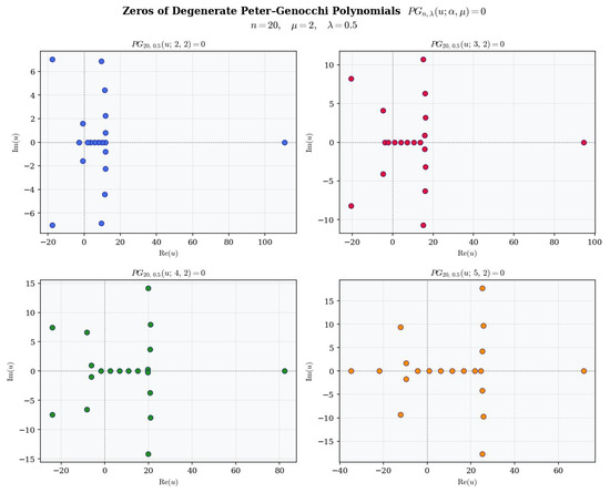
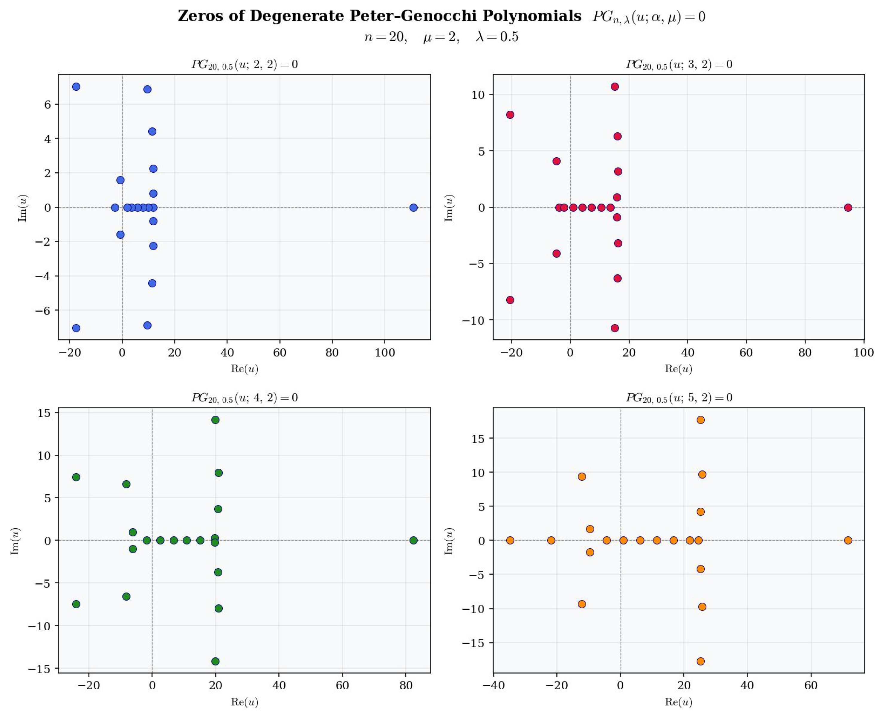
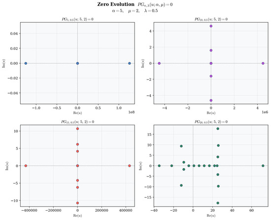
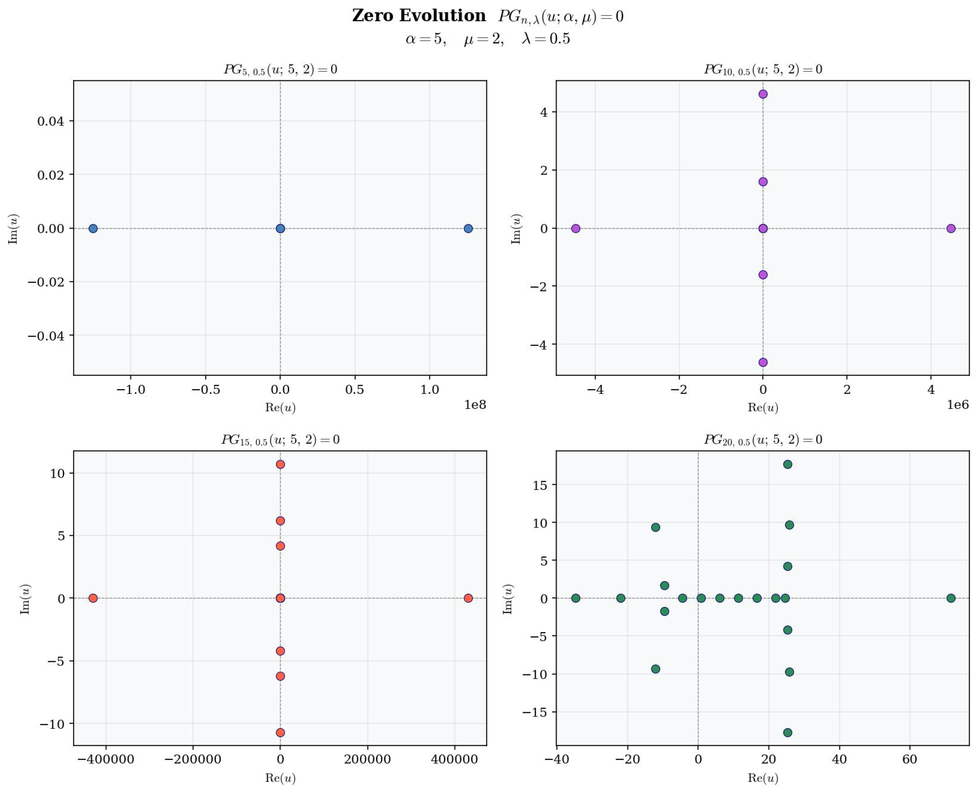
Computational methodology. The zeros listed in Table 1 and displayed in Figure 1, Figure 2, Figure 3 and Figure 4 were computed numerically as follows. For each fixed set of parameters $(\alpha ,\mu ,\lambda )$, we first evaluate the coefficients of $P{G}_{n,\lambda }(u;\alpha ,\mu )$ as a polynomial in u using the recurrence implied by the generating Function (12). The zeros are then obtained via the companion matrix (eigenvalue) method for polynomial root-finding, which reduces the problem to computing eigenvalues of the companion matrix associated with the polynomial. All computations were performed in Python (version 3.11.9) with NumPy (version 1.26.4) using numpy.polynomial and numpy.roots, and the plots were generated using matplotlib (version 3.8.4).

Figure 1. Zeros of $P{G}_{n,\lambda }(u;\alpha ,\mu )=0$, $n=20$, $\mu =2$, $\lambda =0.5$, $\alpha =2,3,4,5$.

Figure 2. Zero evolution, $\alpha =5$, $\mu =2$, $\lambda =0.5$, $n=5,10,15,20$.

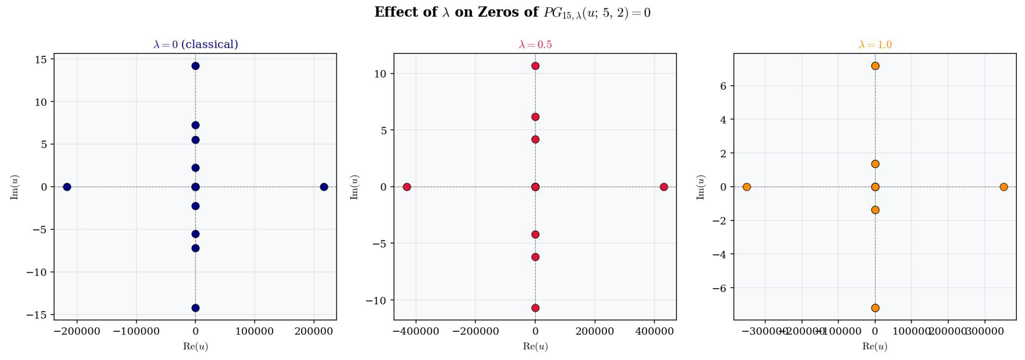
Figure 3. Effect of $\lambda$ on zeros of $P{G}_{15,\lambda }(u;5,2)=0$: $\lambda =0$ (classical), $\lambda =0.5$, $\lambda =1.0$.

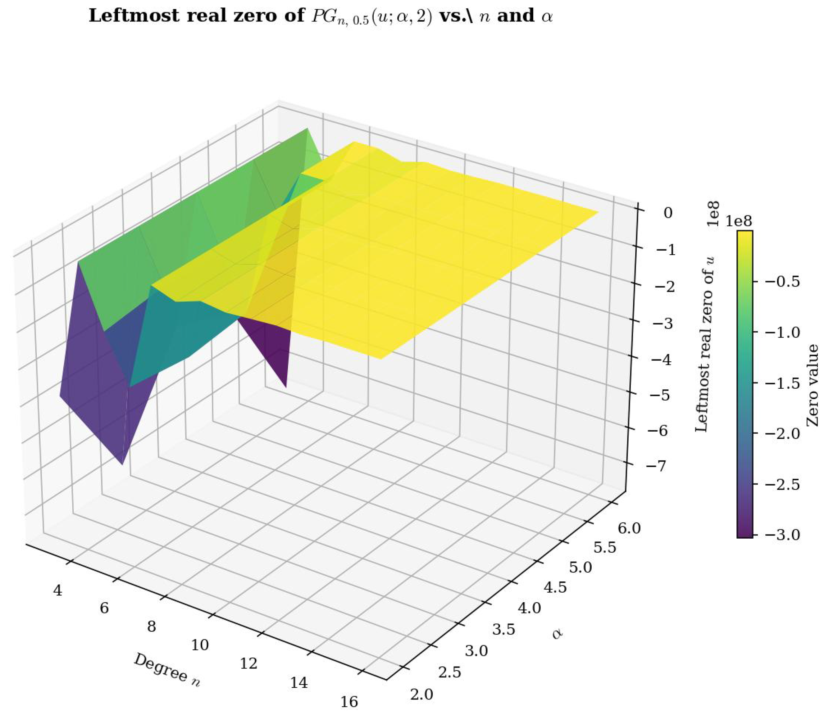
Figure 4. Leftmost real zero of $P{G}_{n,0.5}(u;\alpha ,2)$ as a function of n and $\alpha$.

Remark on the number of zeros in Table 1. For the parameter choice $\mu =2$, $\lambda =0.5$, the first two degenerate Peter–Genocchi polynomials vanish identically: $P{G}_{0,\lambda }(u;\alpha ,2)=0$ and $P{G}_{1,\lambda }(u;\alpha ,2)=0$ (as seen from the explicit list above, and confirmed by the generating Function (12): since ${\left({log}_{\lambda }(1+\tau )\right)}^{\mu }$ contributes a factor of order ${\tau }^{\mu }={\tau }^2$ at leading order when $\mu =2$, the coefficients of ${\tau }^0/0!$ and ${\tau }^1/1!$ in the generating series are identically zero). Consequently, for degree n with $\mu =2$, the polynomial $P{G}_{n,\lambda }(u;\alpha ,2)$ has effective degree $n-2$ in u (the two lowest-order terms are absent), and therefore has exactly $n-2$ zeros counted with multiplicity in $\mathbb{C}$, by the fundamental theorem of algebra. This explains why Table 1 lists $n-2$ approximate zeros for each row of degree n: the companion matrix method is applied to the reduced degree-$(n-2)$ polynomial and returns exactly $n-2$ eigenvalues. More generally, for parameter $\mu$, the first $\mu$ polynomials $P{G}_{0,\lambda },\dots ,P{G}_{\mu -1,\lambda }$ vanish identically, so the effective degree is $n-\mu$ and the method yields exactly $n-\mu$ roots.

Figure 1, Figure 2, Figure 3 and Figure 4 present the zero distributions graphically; Table 1 lists approximate zeros.

Description of Figure 1. Figure 1 displays the zeros of $P{G}_{20,0.5}(u;\alpha ,2)$ in the complex u-plane for four values of $\alpha$. As $\alpha$ increases, the real parts of the zeros spread over a wider interval and the complex conjugate pairs move further from the real axis. For each $\alpha$, the zeros exhibit an approximate symmetry about a central real value, reflecting the quasi-symmetric structure of the polynomial coefficients.

Description of Figure 2. Figure 2 shows the evolution of zeros as the degree n increases from 5 to 20, with $\alpha =5$, $\mu =2$, $\lambda =0.5$. At low degrees ($n=5$), all zeros are real. As n increases, complex conjugate pairs emerge; these pairs migrate further from the real axis with increasing n, while new real zeros continue to appear. This transition from purely real to mixed real–complex zero configurations is a characteristic feature of the degenerate Peter–Genocchi polynomials.

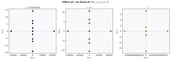
Description of Figure 3. Figure 3 compares the zeros of $P{G}_{15,\lambda }(u;5,2)$ for three values of $\lambda$: the classical case $\lambda =0$ and the degenerate cases $\lambda =0.5$ and $\lambda =1.0$. As $\lambda$ increases from 0, the zeros undergo a continuous deformation: real zeros shift along the real axis, and the imaginary parts of complex conjugate pairs change. This illustrates how the degeneration parameter $\lambda$ controls the deviation from the classical Peter–Genocchi polynomial zeros.

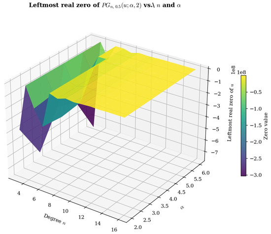
Description of Figure 4. Figure 4 presents a 3D surface plot showing how the leftmost real zero of $P{G}_{n,0.5}(u;\alpha ,2)$ varies as a function of the degree n (horizontal axis) and the parameter $\alpha$ (depth axis). The vertical axis and colour scale both represent the value of the leftmost real zero. The surface reveals that the leftmost real zero decreases (becomes more negative) as n increases and as $\alpha$ increases, exhibiting a monotonic trend in both variables. This suggests that the zero distribution expands along the negative real axis as the polynomial degree and the parameter $\alpha$ grow.

6. Conclusions

In this paper, we introduced the degenerate Peter–Genocchi polynomials $P{G}_{n,\lambda }(u;\alpha ,\mu )$, a new class of special polynomials defined via the generating Function (12) that unifies two independent lines of research: the theory of Peter (higher-order Boole) polynomials and the degenerate polynomial framework. The main contributions of this work are as follows.

We established a comprehensive set of algebraic identities: a summation formula expressing the polynomials in terms of their associated numbers and degenerate falling factorials (Theorem 1); addition formulas that decompose the polynomial argument using degenerate Stirling numbers of the first kind (Theorem 2); an implicit summation formula providing a bivariate convolution identity with the correct degenerate falling factorial ${(u-w)}_{n+m,\lambda }$ (Theorem 3); and two symmetric identities (Theorems 4 and 5).

We derived explicit relations connecting the degenerate Peter–Genocchi polynomials with several important degenerate polynomial families: the degenerate Stirling numbers of the first kind (Theorem 6), the higher-order degenerate Genocchi polynomials via degenerate Stirling numbers of both kinds (Theorems 7 and 8), and the higher-order degenerate Daehee polynomials (Theorem 9).

We investigated derivative properties, obtaining an exact degenerate derivative formula with the correct ${\lambda }^{k-1}$ factor (Theorem 10(i)), a raising-order formula (Theorem 10(ii)), and a differential operator formula using the degenerate differential operator (Theorem 12). The $\alpha$-derivative formula (Theorem 11) was shown to hold exactly in the classical case $\lambda =0$ and approximately for $\lambda \ne 0$, with the precise characterisation of the correction terms left as an open problem.

Finally, we presented a graphical analysis of the zero distributions in the complex plane, illustrating the effects of the degree n, the parameter $\alpha$, and the degeneration parameter $\lambda$ on the structure and migration of zeros.

Several directions for future research emerge naturally from this work: (i) establishing q-analogues of the degenerate Peter–Genocchi polynomials; (ii) investigating p-adic integrals and their connections with this polynomial family; (iii) exploring orthogonality properties and recurrence relations; (iv) providing a complete rigorous proof (or precise correction formula) for Theorem 11 in the case $\lambda \ne 0$; and (v) developing applications in combinatorics and mathematical physics.

References

- Araci, S. Novel identities involving Genocchi numbers and polynomials arising from applications of umbral calculus. Appl. Math. Comput. 2014, 233, 599–607. [Google Scholar] [CrossRef] [Scilit]
- Horadam, A.F. Genocchi polynomials. In Proceedings of the Fourth International Conference on Fibonacci Numbers and Their Applications; Kluwer: Dordrecht, The Netherlands, 1991; pp. 145–166. [Google Scholar]
- Kim, B.M.; Jeong, J.; Rim, S.H. Some explicit identities on Changhee-Genocchi polynomials and numbers. Adv. Differ. Equ. 2016, 2016, 202. [Google Scholar] [CrossRef] [Scilit]
- Kim, B.M.; Jang, L.C.; Kim, W.; Kwon, H.-I. Degenerate Changhee-Genocchi numbers and polynomials. J. Inequal. Appl. 2017, 2017, 294. [Google Scholar] [CrossRef] [Scilit]
- Liu, L.; Wuyungaowa. A note on higher order degenerate Changhee-Genocchi numbers and polynomials of the second kind. Symmetry 2023, 15, 56. [Google Scholar] [CrossRef] [Scilit]
- Wani, S.A.; Patil, S.; Ramírez, W.; Hernández, J. Some families of differential equations for multivariate hybrid special polynomials associated with Frobenius-Genocchi polynomials. Eur. J. Pure Appl. Math. 2025, 18, 5575. [Google Scholar] [CrossRef] [Scilit]
- Wani, S.A.; Shah, T.U.R.; Ramírez, W.; Cesarano, C. Exploring the properties of multivariable Hermite polynomials in relation to Apostol-type Frobenius-Genocchi polynomials. Georgian Math. J. 2025, 32, 515–528. [Google Scholar]
- Duran, U.; Kızılateş, C.; Ramírez, W.; Cesarano, C. A new class of degenerate unified Bernoulli–Euler Hermite polynomials of Apostol type. AIMS Math. 2025, 10, 16117–16138. [Google Scholar] [CrossRef] [Scilit]
- Cesarano, C.; Kızılateş, C.; Hernández, J.; Quiñones, Y.; Ramírez, W. On mixed-type generalized degenerate Lucas–Bernoulli/Euler polynomials. Dolomites Res. Notes Approx. 2026, 19, 82–96. [Google Scholar] [CrossRef]
- Wani, S.A.; Riyasat, M. Integral transforms and extended Hermite-Apostol type Frobenius-Genocchi polynomials. Kragujev. J. Math. 2024, 48, 41–53. [Google Scholar]
- Cesarano, C.; Quintana, Y.; Ramírez, W. Degenerate versions of hypergeometric Bernoulli–Euler polynomials. Lobachevskii J. Math. 2024, 45, 3509–3521. [Google Scholar] [CrossRef] [Scilit]
- Zayed, M.; Wani, S.A.; Oros, G.I.; Ramírez, W. Unraveling multivariable Hermite-Apostol-type Frobenius-Genocchi polynomials via fractional operators. AIMS Math. 2024, 9, 17291–17304. [Google Scholar] [CrossRef] [Scilit]
- Duran, U. Boole Genocchi polynomials. In Proceedings of the 1st BILSEL International Çatalhöyük Scientific Research Congress, Konya, Türkiye, 28–29 October 2023; pp. 306–316. [Google Scholar]
- Duran, U.; Acikgoz, M. The Boole polynomials associated with the p-adic gamma function. Publ. Inst. Math. 2019, 106, 105–112. [Google Scholar] [CrossRef] [Scilit]
- Kim, D.S.; Kim, T. A note on Boole polynomials. Integral Transform. Spec. Funct. 2014, 25, 627–633. [Google Scholar] [CrossRef] [Scilit]
- Kim, D.S.; Kim, T. Generalized Boole numbers and polynomials. Rev. Real Acad. Cienc. Exactas Fís. Nat. Serie A Mat. 2016, 110, 823–839. [Google Scholar] [CrossRef] [Scilit]
- Li, Y.-W.; Dağlı, M.C.; Qi, F. Two explicit formulas for degenerate Peters numbers and polynomials. Discret. Math. Lett. 2022, 8, 1–5. [Google Scholar]
- Simsek, Y.; So, J.S. On generating functions for Boole type polynomials and numbers of higher order and their applications. Symmetry 2019, 11, 352. [Google Scholar] [CrossRef] [Scilit]
- Simsek, Y. A new family of combinatorial numbers and polynomials associated with Peters numbers and polynomials. Appl. Anal. Discret. Math. 2020, 4, 627–640. [Google Scholar] [CrossRef] [Scilit]
- Duran, U.; Acikgoz, M.; Khan, W.A.; Ryoo, C.S. Some properties of the Peter-Genocchi polynomials with location of their zeros. Konuralp J. Math. 2026, 14, 142–154. [Google Scholar]
- Carlitz, L. Degenerate Stirling, Bernoulli and Eulerian numbers. Util. Math. 1979, 15, 51–88. [Google Scholar]
- Kim, T. q-Volkenborn integration. Russ. J. Math. Phys. 2002, 9, 288–299. [Google Scholar]
- Kim, T.; Kim, D.S. Degenerate Laplace transform and degenerate gamma function. Russ. J. Math. Phys. 2017, 24, 241–248. [Google Scholar] [CrossRef] [Scilit]
- Kim, D.S.; Kim, T.; Seo, J.J.; Lee, S.-H. Higher-order Changhee numbers and polynomials. Adv. Stud. Theor. Phys. 2014, 8, 365–373. [Google Scholar] [CrossRef] [Scilit]
- Wang, N.L.; Li, H. Some identities on the higher-order Daehee and Changhee numbers. Pure Appl. Math. J. 2015, 4, 33–37. [Google Scholar]
- Fadel, M. Degenerate generalized Hermite polynomials: Operational and monomiality properties. Adv. Stud. Contemp. Math. 2026, 36, 119–135. [Google Scholar]
- Rudin, W. Principles of Mathematical Analysis, 3rd ed.; McGraw-Hill: New York, NY, USA, 1976. [Google Scholar]
- Kim, T.; Kim, D.S. On some degenerate differential and degenerate difference operators. Russ. J. Math. Phys. 2022, 29, 37–46. [Google Scholar] [CrossRef] [Scilit]
Disclaimer/Publisher’s Note: The statements, opinions and data contained in all publications are solely those of the individual author(s) and contributor(s) and not of MDPI and/or the editor(s). MDPI and/or the editor(s) disclaim responsibility for any injury to people or property resulting from any ideas, methods, instructions or products referred to in the content. |
© 2026 by the authors. Licensee MDPI, Basel, Switzerland. This article is an open access article distributed under the terms and conditions of the Creative Commons Attribution (CC BY) license.