


Abstract
This paper develops a geometric framework for analyzing the ideal structure of the bipolar semigroup under coordinate-wise addition. Subsets of B are interpreted as planar regions, allowing ideals to be described in terms of boundary behavior. In particular, we prove that the complement of a simply connected region is an ideal of the commutative additive semigroup if and only if its boundary contains no strictly decreasing segment. This provides a direct and visually verifiable criterion for ideality, linking algebraic structure to geometric shape. Each ideal can be written as a union of translates of the form , with minimal generating sets determined by boundary structure. Potential applications to modeling bipolar system states, including cybersecurity contexts, are also discussed. These results uncover an intrinsic symmetry between algebraic closure and geometric monotonicity, offering a new perspective on semigroup ideals through spatial structure. In contrast to our previous work on the semiring , where ideals necessarily exhibit symmetry with respect to the line , we show that removing the multiplicative operation leads to a fundamentally different geometric behavior: ideals in the semigroup no longer possess symmetric shapes. This demonstrates that the multiplicative structure is the key mechanism enforcing geometric symmetry.
1. Introduction
Ideal theory is a fundamental part of algebra and plays an essential role in the study of semigroup structure, including decomposition, regularity, and classification. In classical semigroup theory, ideals are widely used to describe internal algebraic properties. A key contribution in this direction was made by A.H. Clifford [1], who studied semigroups without nilpotent ideals. His work established the conditions under which ideal structures change and confirmed that ideals are central objects in abstract semigroup theory. Later studies expanded these classical ideas to specific types of semigroups. For example, M.A. Reynolds and R.P. Sullivan [2] investigated ideals in transformation semigroups generated by idempotents. Similarly, P. Honyam and J. Sanwong [3,4] analyzed ideal structures in transformation semigroups with invariant and fixed sets. These researchers showed how ideals interact with generators and Green’s relations, proving that algebraic and combinatorial methods are effective tools for describing these structures.
In recent years, various generalized notions of ideals have been introduced to provide simpler or more flexible characterizations [5,6]. This includes the introduction of new concepts such as -ideals and -quasi-ideals [7]. With the growth of fuzzy algebra, ideal theory has also been extended to fuzzy semigroups. This has led to the development of fuzzy ideals, quasi-ideals, and bi-ideals as generalizations of classical concepts. Detailed overviews of this transition from classical to fuzzy semigroups can be found in [8]. Additionally, the study of fuzzy and soft semigroups has produced variants such as soft ideals [9,10], while rough set theory has introduced rough interior and rough quasi-ideals [11]. Finally, generalized fuzzy ideals in ordered semigroups were explored in [12]. This research demonstrated that such ideals are useful for examining the properties of ordered semigroups and can even be applied to decision-making models.
Alongside these developments, new generalizations of ideal theory have been proposed within more flexible frameworks. A different perspective is found in bipolar quantum linear algebra (BQLA). The bipolar set, defined as
was introduced by W.R. Zhang to address concepts in quantum theory and was later expanded into a bipolar quantum linear algebra framework [13,14]. Bipolar fuzzy set theory has emerged as an extension of classical fuzzy logic that allows the simultaneous representation of both positive and negative information, and has been applied to various algebraic structures. For example, the notion of bipolar fuzzy commutative ideals in BCK-algebras was developed by A. Almuhaimeed and H. Alshehri [15], offering a mathematical framework that simultaneously captures positive membership and negative non-membership information. Their study established key theoretical properties and demonstrated that bipolar fuzzy commutative ideals form a proper subclass of bipolar fuzzy ideals, with equality holding only in commutative BCK-algebras. This algebraic framework offers promising applications in decision-making and soft computing, especially where processing bidirectional uncertainty is required. Beyond algebraic settings, recent research has extended bipolar fuzzy set theory to topological frameworks. Researchers introduced bipolar fuzzy supra topologies along with neighborhood and Q-neighborhood systems [16]. Their approach extends traditional topological concepts by incorporating positive and negative membership degrees, enabling more nuanced handling of uncertainty and imprecision. Its practical effectiveness was further demonstrated through a data mining reduction algorithm that successfully processes datasets with missing attribute values, as validated by numerical examples.
Although these developments greatly expand the use of ideal theory, existing research has mostly focused on internal algebraic properties. Most current approaches do not include a geometric interpretation of the underlying structures. In particular, the role of boundary behavior and geometric properties in characterizing ideals has not yet been systematically studied.
The bipolar semigroup , using coordinate-wise addition, is a commutative and cancellative semigroup that can be viewed as part of the Euclidean plane. This observation suggests that ideal theory in may follow geometric principles rather than just algebraic ones. The main goal of this paper is to investigate the ideal structure of the bipolar semigroup from a geometric perspective and to answer the following question:
This paper fills this gap by developing a geometric characterization of ideals in the bipolar semigroup . Our main result, Theorem 8, shows that the complement of a simply connected region in B is an ideal if and only if its boundary contains no strictly decreasing segments. The advantage of this framework is that it reformulates ideal theory in a geometric way. By defining ideality through the boundary behavior of planar regions, we provide an intuitive alternative to traditional algebraic proofs. Our results show that the absence of strictly decreasing boundary segments is a clear and complete condition for ideality. This allows for a quick geometric inspection: any strictly decreasing part of a boundary immediately means the region is not an ideal. However, certain limitations exist. While the theory effectively characterizes ideals generated by regions and rectangles, visualizing boundaries for highly irregular or arbitrary generating sets can be technically demanding. In these cases, applying the geometric criterion may be more technically challenging. Despite these limitations, this paradigm offers a strong foundation for understanding invariant structures in bipolar systems through a visual, coordinate-based approach.“Under what geometric conditions does a subset of the bipolar semigroup form an ideal in ?”
Building on the geometric interpretation of ideality in the bipolar semigroup, this paper considers the shift from a semiring structure to a purely additive semigroup, that is, the absence of multiplicative interaction. The results show that this structural reduction does not only lead to technical modifications, but also produces significantly different geometric behavior, proof methods, and conceptual objectives when compared with our earlier work on bipolar semirings [17]. These differences can be summarized into three main aspects, as described below.
- Geometric Structure: In the previous work, ideals are constrained to specific symmetric patterns, typically characterized as V-shaped relative to . In contrast, this paper reveals that ideals in bipolar semigroups do not have a fixed global shape. Instead, we propose a geometric characterization based on their core components, identified as translated regions .
- Methodological Tools: Our previous methodology relied on infimum properties to show that semiring ideals are generated by a single point. However, this paper demonstrates that a semigroup ideal I must be represented as an arbitrary union of translated regions. To achieve this, we utilize the intermediate value theorem as a core analytical tool to prove the existence of an index set M within the boundary of I. This represents a significant methodological departure, as such tools were not applicable in the prior semiring study.
- From Classification to Construction: For the semiring B, we provided necessary and sufficient conditions for the ideals of B generated by A, which can be classified into only three types: linear , V-shaped, or the whole space. Because the semigroup structure lacks multiplication, the resulting ideal forms are far more diverse. Consequently, this paper shifts from simple classification to a rigorous construction proof for a minimal index set M, providing a more comprehensive understanding of these complex substructures.
This paper is organized as follows. Section 1 introduces the problem and motivation of the study. Section 2 presents the preliminary definitions and terminology. Section 3 develops the main results concerning the geometric properties of ideals in the semigroup . Section 4 concludes the paper, and Section 5 outlines directions for future research.
2. Preliminaries
To answer the question raised in the introduction, we first review the basic definitions of semigroup theory. For a more detailed explanation of these concepts, we refer the reader to the standard text [18] and the research in [19].
Let X and Y be nonempty subsets of a semigroup S. We define the subset of S as:
Definition 1
([18]). Let I be a nonempty subset of a semigroup S.
- 1.
- I is called a left ideal of S if .
- 2.
- I is called a right ideal of S if .
- 3.
- I is called a two-sided ideal (or simply an ideal) of S if it is both a left and a right ideal.
In the case where S is commutative, the concepts of left ideals, right ideals, and two-sided ideals coincide.
Next, we introduce the definitions relevant to our study, specifically those related to bipolar structures. These definitions are adapted from the work of Zhang [20].
Definition 2.
The bipolar set B is defined as the set of pairs:
where denotes the set of non-negative real numbers.
The interior of B is
Definition 3.
Consequently, is a commutative semigroup with the identity element . Because it is commutative, the definitions of left, right, and two-sided ideals are identical. Furthermore, is a cancellative semigroup, although it is not a group because its elements do not have inverses.Let . Then the addition is a binary operation on B and is defined as
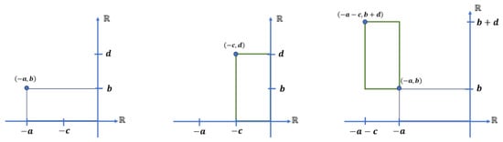
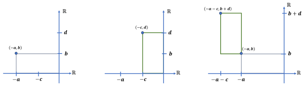
with as an identity element, see Figure 1. The addition has commutative, associative, and cancellation properties.
Figure 1.
The addition of two elements in B, where .
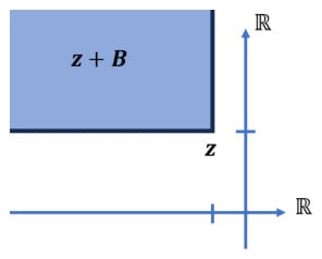
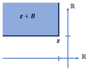
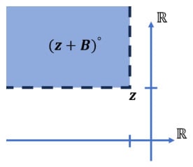
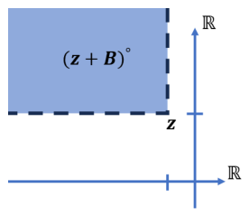
Based on the addition of and , the result represents a point that can be visualized as the upper-left corner of a rectangle, as shown in Figure 1 (right). In other words, the position of is exactly c units to the left and d units above the point . For any element in B, the translate plays a fundamental role in the ideal structure of the semigroup . Subsets of this form create a natural class of ideals that are easy to understand geometrically. Figure 2 illustrates this structure.
Figure 2.
The region , representing a translation of the semigroup B by the element z. Geometrically, it forms an upper-left translated region unbounded to the left and upward.
Representing B in the Euclidean plane creates a natural link between algebra and geometry. In this view, subsets of B are regarded as regions in the plane, and their algebraic behavior is closely related to the shape of their boundaries. This geometric viewpoint provides a basis for studying ideals in through boundary behavior.
The remainder of this section is devoted to a geometric interpretation behind the ideal characterization developed below. This interpretation follows naturally from the definition of an ideal in Definition 1 together with the definition of addition in Definition 3, illustrated in Figure 1.
Let I be an ideal of B. Since , for any and , it follows that
Geometrically, the point lies a units to the left and b units above the point . The following boundary cases illustrate the geometric nature of this closure property. If , then
which gives an unbounded upward ray contained in I. Similarly, if , then
which gives an unbounded leftward ray contained in I. More generally, for every ,
Hence, by the nature of the addition operation (see Figure 1), each point of an ideal generates an upper-left translated region, unbounded to the left and upward, that is contained in the ideal. This observation shows that the ideal structure of B is governed by the boundary behavior of such regions.
3. Main Results
3.1. Structural Characterizations of and
We begin by investigating the structure of ideals within the bipolar set B under the operation of addition.
Theorem 1.
For each , the following statements hold:
- 1.
- The set is a closed ideal of B.
- 2.
- The set is an open ideal of B.
Proof.
- 1.
- Clearly, is a closed subset of B. Let and define . To show that , let and , where and . By the definition of addition (see Figure 1), the point lies a units to the left and b units above . Since , it follows that and . Therefore, and , which implies that .
- 2.
- Clearly, is an open subset of B. Let and define . The proof that is analogous to (1.), using strict inequalities instead. Indeed, if and , then and , which imply that and . Hence, .
□
Remark 1.
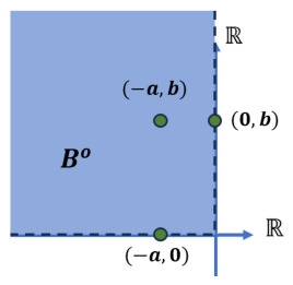
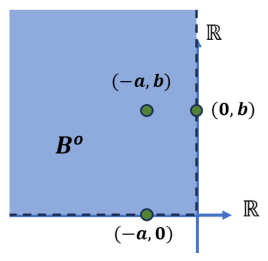
The geometric meaning of this result is that each translate corresponds to a copy of the bipolar set B shifted so that its vertex is located at z. Similarly, corresponds to the same shifted region with its boundary removed; see Figure 2 and Figure 3.
Figure 3.
Geometric representation of the set of all interior points of , denoted by .
According to Theorem 1 and the properties of ideals, arbitrary unions of sets of the form or are ideals of B.
Theorem 2.
Let I be a subset of the semigroup . Then the following statements hold:
- 1.
- I is an ideal of B if and only if there exists a subset such thatMoreover, one may choose .
- 2.
- If there exists a finite subset such that , then I is closed ideal of B.
- 3.
- If there exists a subset such that , then I is an open ideal of B.
Proof.
- 1.
- Only the sufficiency requires proof. Let I be an ideal of and set . Since ,Conversely, as ,Therefore, .
- 2.
- The conclusion follows from the fact that a finite union of closed sets is closed.
- 3.
- The conclusion follows from the fact that an arbitrary union of open sets is open.
□
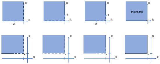
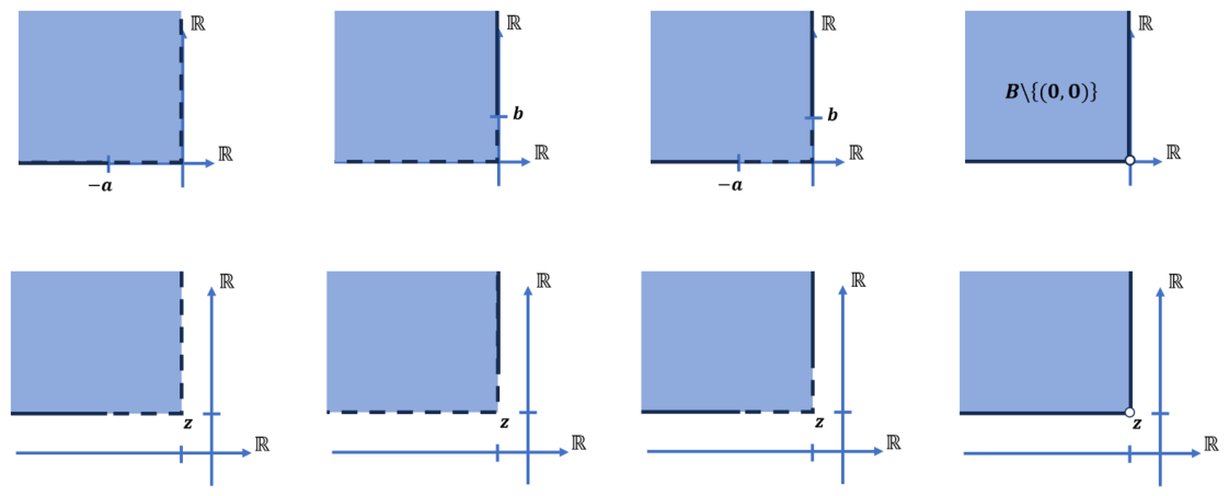
By summarizing the structure of ideals in the semigroup B. According to Theorem 2, every ideal can be expressed as an arbitrary union of the sets illustrated in Figure 4. Their classification into open and closed sets is summarized in Table 1.
Figure 4.
Trivial patterns of ideals in the semigroup B. Any ideal in B can be represented as a union of these fundamental forms.
Table 1.
Open and closed sets in the semigroup B.
Remark 2.
By Theorem 1, the set
is an ideal of B. Moreover, if there exists such that
or there exists such that
then the ideal is neither open nor closed.
Figure 5.
The ideal .
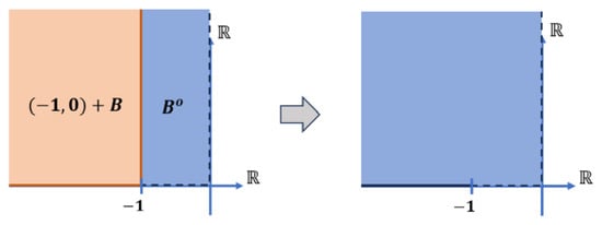
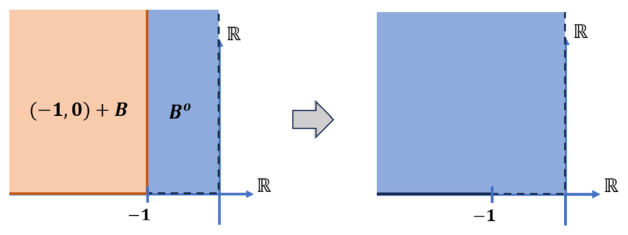
Similarly, the ideal corresponds to the right-hand panel in Figure 6.
Figure 6.
The ideal .
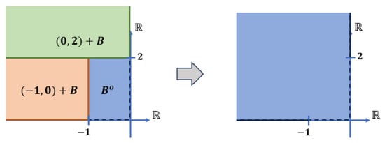
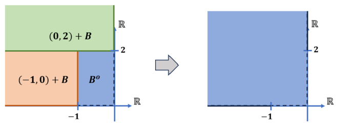
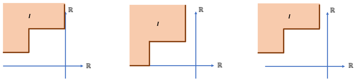
The same construction yields eight elementary patterns of ideals in the semigroup B that are neither open nor closed, as illustrated in Figure 7. They are described as follows.
Figure 7.
Elementary ideal patterns in the semigroup B that are neither open nor closed.
Definition 4
([21]). A space X is said to be simply connected if it is path-connected and if is the trivial group for some , and hence for every .
In planar topology, a simply connected region contains no holes and consists of a single connected piece [22], p. 1078.
In general, an arbitrary union of simply connected sets need not be simply connected. However, the particular geometric structure of each set guarantees that the union is always simply connected. Consequently, Theorem 2 implies that every ideal of B is simply connected.
Theorem 3.
If I is an ideal of B, then I is simply connected.
Proof.
Let I be an ideal of B, and let with . Without loss of generality, assume that and . Let be the line segment joining to , and let be the line segment joining to . Then
Since , it follows that . Hence, defines a path in I connecting and . Therefore, I is path-connected, and consequently a connected set.
By Theorem 2, every ideal I can be represented as an arbitrary union of sets of the form , where . Each region is an upper-left translated region, unbounded to the left and upward, and contains no holes (see Figure 2). Consequently, the union also contains no holes. Therefore, I is simply. □
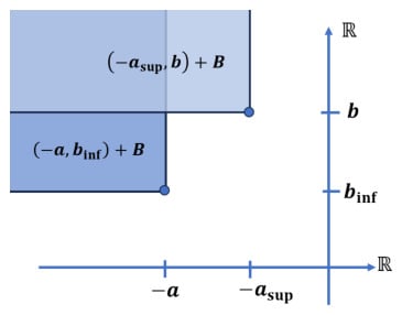
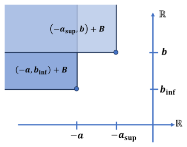
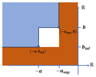
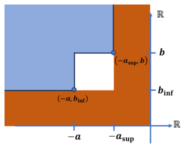
The representation in Theorem 2 is generally not unique; see Example 1. A more precise description of ideals can be obtained by choosing a suitable generating subset . In this work, the set M is related to a certain part of the boundary of I, denoted by L. Furthermore, we show that I cannot be an ideal if L satisfies certain geometric conditions. Henceforth, let R be an open and simply connected region bounded by a curve L, the x-axis, and the y-axis. The geometric properties of L are determined by the boundary of R within B; visual representations of these behaviors are provided in Figure 8, Figure 9, Figure 10, Figure 11, Figure 13 and Figure 14. Specifically, we explore how the complement may form an ideal depending on the structural characteristics of L.
3.2. Ideals of the Form
Theorem 4.
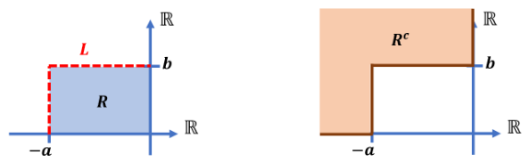
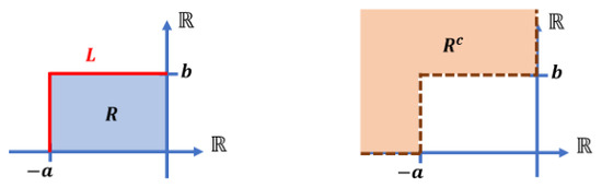
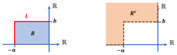
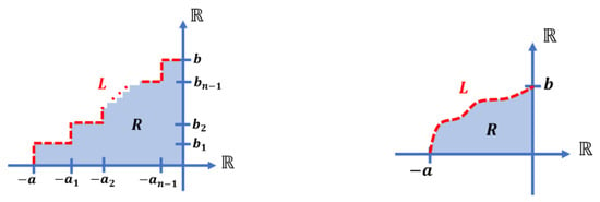
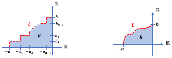
If L is the set , then is an ideal of the semigroup . Moreover, , where ; see Figure 8.
Figure 8.
The region defined in Theorem 4: (left) R, (right) .
Proof.
Therefore, .
Hence, . Consequently, is an ideal of .
Let and . We consider two cases.
- Case 1.
- . Since , it follows that , and hence
- Case 2.
- . Then . Since , we have , which implies
Choose . We will show that . Since
and
we get . Conversely, let , and we consider two cases of b.
- Case 1.
- . Then and then
- Case 2.
- . We have and then
□
Remark 3.
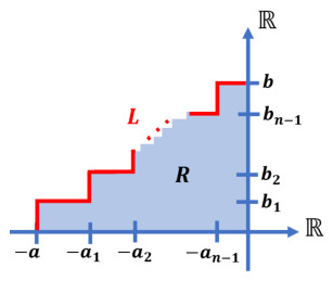
According to Theorem 4, suppose the boundary curve L is defined by the union . Here, each is given by
where , , , and ; see Figure 9.
Figure 9.
The region R as defined in Remark 3.
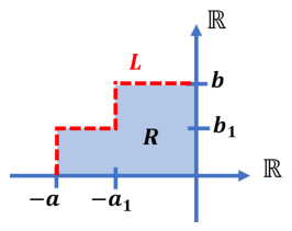
In this case, we may select the generating set . Furthermore, by applying the same reasoning used in the proof of Theorem 4, it follows that . This set constitutes an ideal of the semigroup .
These observations provide the motivation for the following result.
Theorem 5.
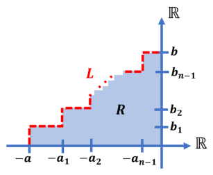
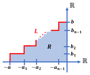
Let
where
with , , , and ; see Figure 10. Then there exists a set M such that is an ideal of . Moreover, one may choose
Figure 10.
The region R as described in Theorem 5.
Theorem 6.
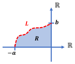
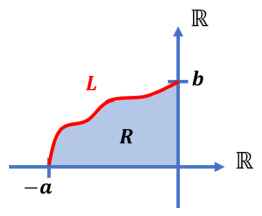
Let L be the graph of a strictly increasing and continuous function such that and ; see Figure 11. Then is an ideal of a semigroup .
Figure 11.
The region R as described in Theorem 6.
Proof.
Assume, therefore, that . Since , we have .
By the boundary condition and the strict monotonicity of L, we have for all . It remains to prove the reverse inclusion. Let .
- Case 1.
- Suppose that . Since and , we have
- Case 2.
- Suppose that . Since and , we have
- Case 3.
- Suppose that and . If , then
For , define
Since , we obtain
By the intermediate value theorem, there exists such that . Hence
and therefore
Since , we have
□
Remark 4.
If the strictness condition for the curve L is omitted in Theorem 6, we can apply Theorem 5 to show that constitutes an ideal of B, where .
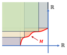
From Theorem 4 to Theorem 6, without assuming minimality, the set M coincides with the set of convex corners of L; see Figure 12.
Figure 12.
M is the set of convex corners of L.
Corollary 1.
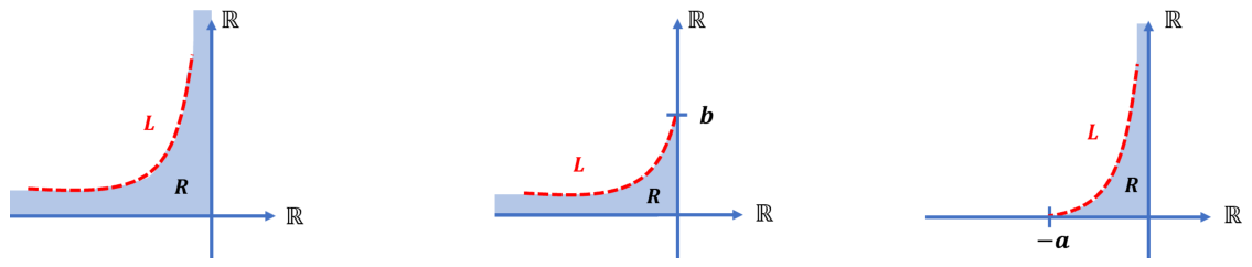
Let L be the graph of an increasing and continuous function . Then is an ideal of a semigroup provided that one of the following conditions holds (see Figure 13 for illustrations):
- 1.
- and .
- 2.
- , , and .
- 3.
- , , and .
Proof.
- 1.
- By the same argument used in Case 3 of the proof of Theorem 6.
- 2.
- By the same argument used in Cases 2 and 3 of the proof of Theorem 6.
- 3.
- By the same argument used in Cases 1 and 3 of the proof of Theorem 6.
□
Figure 13.
The region R as described in Corollary 1.
Based on Theorems 5 and 6, the case where f is non-decreasing has been characterized. We now consider the structure of the ideal I when f is not non-decreasing.
The following definition introduces terminology that plays an important role in the main results.
Definition 5.
Let be a boundary curve. We say that L contains a strictly decreasing segment if a segment of L can be represented by for , and there exist such that .
Theorem 7.
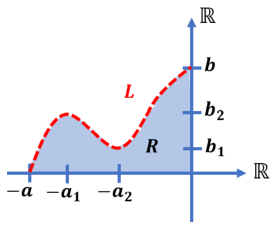
Let L be a boundary curve containing a strictly decreasing segment, and let be the region bounded by L and the coordinate axes; see Figure 14. Then is not an ideal of .
Figure 14.
The region R as described in Theorem 7.
Proof.
Since L contains a strictly decreasing segment, there exist such that . Choose a point satisfying . Then , since it lies above the boundary at . On the other hand, the point lies below the boundary at , and hence .
Set . Then , and
where . Thus, , and . Therefore, , and so is not an ideal. □
According to Theorems 4–7, and particularly Theorems 5 and 6, the index sets are not unique; however, each such set is minimal. These observations lead to the following theorem:
Theorem 8.
There exists a minimal set such that is an ideal of the semigroup if and only if the boundary curve L contains no strictly decreasing segment.
Remark 5.
This result indicates that strictly decreasing boundary segments are the only obstruction to the ideality of . Specifically, if L is non-decreasing, then is an ideal; otherwise, it is not.
The following example provides further insight into Theorem 8.
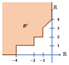
Example 1.
Moreover, , where
By Theorem 2, one may also choose . Alternatively, M may be taken as the set of convex corners of L.
From Theorem 8 and Figure 15, is an ideal since its boundary curve contains no strictly decreasing segment.
Figure 15.
An illustration of Example 1.
Beyond this geometric characterization, we may examine the internal structure of such sets through their representations. For any nonempty subset , if X can be expressed as an arbitrary union of sets of the form , then X corresponds to a generating subset . This raises the question: if X is not an ideal, is the set M still related to the elements of X? We investigate this by considering the ideal of the bipolar set B generated by X, as seen in Theorem 9.
For convenience, we let A denote the set , where A is assumed to be nonempty, closed, and connected. Let and be the projections of A onto the x-axis and y-axis, respectively; that is,
Since 0 is an upper bound for and a lower bound for , we define and . Consequently, there exist such that and are elements of , where denotes the set of all boundary points of A.
To gain a deeper understanding of the situation and to further clarify how the following set M is constructed, we analyze the points and in with reference to Theorem 1.
As illustrated in Figure 16 and Figure 17, consider the properties of and . Either
covers A, or some part of A is not covered by In this case, define
Then , and there is no point such that
Consequently, two cases are possible:
or
These conditions lead us to define the set M as follows:
Figure 16.
Geometric representation of the set in the bipolar semigroup B.
Figure 17.
The region .
We are now prepared to investigate the ideal of a bipolar semigroup generated by an arbitrary nonempty set. The formal definition and the corresponding theorem are presented below.
Definition 6
([18]). For each nonempty subset X of a semigroup S, the smallest ideal of S containing X is called the ideal of S generated by X, denoted by .
Theorem 9.
Let A be any nonempty closed and connected subset of the semigroup . Then , where M is defined in Equation (1).
Proof.
and
Let . If , then because is contained within the union of the translates generated by and , both of which are elements of M. For the case where , let L be the horizontal line . This line must intersect the set at some point , which implies . Consequently,
- Case 1.
- . Let as defined in Equation (1). Since and is an ideal, it follows that for each . Thus, . Consequently, we obtain .
- Case 2.
- . We choose . By a similar argument as in Case 1, we have . It remains to show that . Let , where
□
The following example provides further insight into Theorem 9.
Example 2.
Let A denote the region bounded by the ellipse
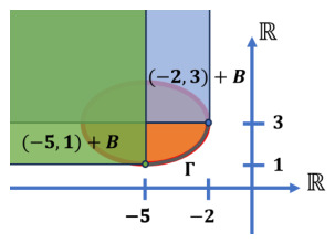
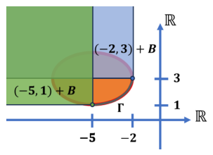
Then A is a nonempty closed and connected set of the semigroup B. From the geometry of the ellipse and its axes, it follows that and . Since
by Theorem 9, we have , where Γ denotes the lower-right arc of the ellipse formed by its major and minor axes; see Figure 18.
Figure 18.
An illustration of Theorem 9 for an elliptical region.
3.3. Ideals of the Form
In this subsection, we let R denote a closed and simply connected region bounded by the curve L, the x-axis, and the y-axis.
Theorem 10.
If L is the set , then is an ideal of the semigroup , where ; see Figure 19.
Figure 19.
The region R as defined in Theorem 10.
Proof.
Since , we have
Hence,
By Theorem 1 (2), each set is an ideal of B. Therefore, is an ideal. □
The following theorem generalizes Theorem 10.
Theorem 11.
Figure 20.
The region R as defined in Theorem 11.
Theorem 12.
Let L be the graph of a strictly increasing and continuous function such that and ; see Figure 21. Then is an ideal of a semigroup .
Figure 21.
The region R as defined in Theorem 12.
Proof.
By the boundary condition and the strict monotonicity of L, we have for all . It remains to prove the reverse inclusion. Let . Then and .
- Case 1.
- Suppose that . Since and , we obtain
- Case 2.
- Suppose that . This follows analogously to Case 2 in Theorem 6, with strict inequalities.
- Case 3.
- Suppose that and . Since is open and , we have . The argument is therefore the same as in Case 3 of Theorem 6. Hence, . □
Theorems 10–12 indicate that removing the boundary of only replaces by . Since the proofs follow the same arguments as those of Theorems 4–6, the following theorem gives the main result for the case of .
Theorem 13.
There exists a minimal set such that is an ideal of the semigroup if and only if the boundary curve L contains no strictly decreasing segment.
3.4. Maximal, Principal, and Prime Ideals of B
In this subsection, we demonstrate that is the unique maximal ideal of and that every proper principal ideal of B has the form , where . Furthermore, no proper ideal of B is both prime and open or closed.
Definition 7
([23]). A proper ideal M of a semigroup S is called maximal if for any ideal I of S implies either or .
Definition 8
([23]). An ideal P of a semigroup S is called prime if implies that or for any ideals of S.
Definition 9
([23]). An ideal P of a semigroup S is called completely prime if implies that or for any elements a and b of S.
While every completely prime ideal is prime, the converse does not necessarily hold. However, these two concepts coincide when the semigroup S is commutative. Although some authors allow the entire semigroup to be considered prime, we restrict our focus to proper prime ideals to establish a nontrivial structural theory.
Definition 10
([18]). An ideal I of a semigroup S is called principal if there exists an element such that , or more simply, , where . Here, denotes the semigroup S with an identity element 1 adjoined if necessary:
From Theorem 1 and Definition 10, it follows that is a principal ideal of B. Moreover, since is a commutative semigroup with identity , and
for every . These observations lead to the following theorem.
Theorem 14.
For each , the set is the unique form of a principal ideal. Consequently, every principal ideal is a closed set.
Theorem 15.
The set is the unique maximal ideal of the semigroup . Moreover, no proper ideal of B is both maximal and open or closed.
Proof.
By Definition 7, the set is a maximal ideal.
Let I be an ideal such that . Then there exists with . Since is an ideal, define
It follows that . Hence, I is not a maximal ideal.
This conclusion applies to every open or closed proper ideal I of B, since such ideals satisfy . Therefore, no open or closed proper ideal of B is maximal. □
The following theorem provides examples of prime ideals that are neither closed nor open.
Theorem 16.
The following sets are prime ideals:
- 1.
- .
- 2.
- .
Proof.
- 1.
- Since I is an arbitrary union of for all , see Figure 7, we get I is an ideal. To show that I is a prime ideal, let such that . Suppose that . Then , and henceIt follows that , and therefore .
- 2.
- The proof is analogous to that of .
□
Theorem 17.
Let I be a closed subset of a semigroup . If I is a proper ideal of B, then I is not a prime ideal.
Proof.
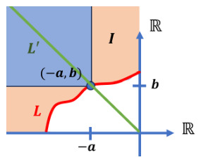
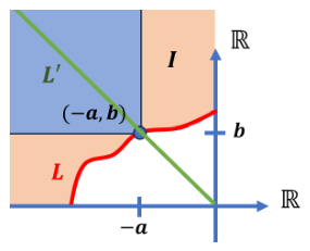
Assume that a proper ideal I is a closed subset of B, and let L be the boundary of I given in Theorem 8. Since is open, it cannot be reduced to a singleton set or to a subset of the x-axis or y-axis. Therefore, contains interior points in the second quadrant away from the coordinate axes. Thus, choose a point with and . Consider the straight line in the bipolar set B. By Theorem 2, we have ; see Figure 22. Hence,
Consequently,
which is nonempty. Therefore, for every . In particular, taking , we obtain . However,
Thus, I is not a prime ideal. □
Figure 22.
An illustration for the proof of Theorem 17.
Theorem 18.
Let I be an open subset of a semigroup . If I is a proper ideal of B, then I is not a prime ideal.
Proof.
If , then I is not a prime ideal, since for any , neither nor belongs to ; see Figure 23. If , then I is an arbitrary union of by Theorem 13. The argument in the proof of Theorem 17 adapts to the case , and hence I is not a prime ideal. □
Figure 23.
An illustration for the proof of Theorem 18.
3.5. Quasi-Ideals and Bi-Ideals of B
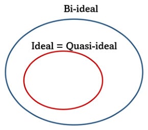
In semigroup theory, various perspectives can be considered. Since is commutative, every quasi-ideal is an ideal. However, we provide explicit examples of bi-ideals that are not quasi-ideals, demonstrating that the class of bi-ideals is strictly larger. We now present the following results, which can be derived in a straightforward manner; for further details, refer to Propositions 2 and 3.
Definition 11
([19]). Let I be a nonempty subset of a semigroup S. Then
- 1.
- I is called a quasi-ideal if .
- 2.
- I is called a bi-ideal if .
Every left ideal and every right ideal of a semigroup is a quasi-ideal.
Definition 12
([18]). A semigroup S is called left [right] simple if S is its only left [respectively, right] ideal. Moreover, S is called simple if it has no proper ideal.
Definition 13
([18]). Let S be a semigroup and . Then
- 1.
- a is called a zero if for every x in S.
- 2.
- a is called regular if for some x in S.
- 3.
- a is called idempotent if .
A semigroup S is called regular if every element of S is regular.
Proposition 1
([19]). Every quasi-ideal of a semigroup is a bi-ideal. Moreover, in a regular semigroup, every bi-ideal is also a quasi-ideal.
Theorem 19
([18]). Let S be a semigroup with identity element e.
- 1.
- The set of all units of S, i.e., is a subgroup of S. We call the group of units of S.
- 2.
- Every subgroup of S containing e is contained in .
Since is a commutative semigroup with identity , the preceding definitions lead to the following properties.
Proposition 2.
The following properties hold for the bipolar semigroup :
- 1.
- The semigroup B has no zero element. The element is the only regular element and the only idempotent in B. Hence, B is not a regular semigroup.
- 2.
- The group of units of B is . Furthermore, the largest subgroup of B containing is the trivial group .
- 3.
- B is not a simple semigroup.
- 4.
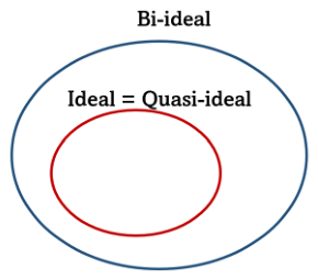
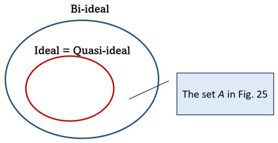
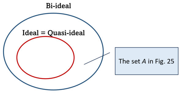
- Every quasi-ideal in B is an ideal (see Figure 24).Figure 24. The relationship between ideals, quasi-ideals, and bi-ideals in .
Proof.
- 1.
- This follows directly from Definition 13. The semigroup B is not regular, since only satisfies ; for each , such an x must be negative, which is not possible.
- 2.
- This is established by Theorem 19.
- 3.
- This is a consequence of Definition 12.
- 4.
- This follows from Definition 11 and the commutativity of .
□
Given Proposition 1 and Proposition 2 (4), it is natural to investigate which subsets of B are bi-ideals but not quasi-ideals.
Proposition 3.
Bi-ideals and quasi-ideals do not coincide in the semigroup .
Proof.
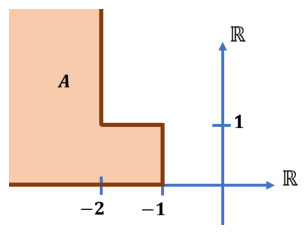
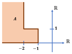
We show that the set A depicted in Figure 25 is a bi-ideal but not a quasi-ideal. Since
is an ideal, by Theorem 1 (see Figure 26 (left)), and , it follows that
Hence, A is not a quasi-ideal.
Figure 25.
An example of a set A that is a bi-ideal but not a quasi-ideal in B.
Figure 26.
Geometric representations: (left) , (middle) , and (right) .
On the other hand, by the commutativity of addition in , the order of summation does not affect the result. Consequently,
(see Figure 26 (middle) and (right)). Therefore, A is a bi-ideal. □
3.6. Algebraic Modeling of Vulnerability and Defense: A Bipolar Semigroup Approach
The geometric characterization of ideals in the bipolar semigroup provides a rigorous algebraic framework for representing system states in complex, adversarial environments, including cyber–physical systems (CPSs) and the Internet of Medical Things (IoMT). Within such domains, security cannot be adequately described as a binary condition (secure vs. insecure); rather, it emerges as a dynamic and continuously evolving property shaped by the interplay between vulnerability exposure and defensive adaptation. Prior work in IoMT cybersecurity highlights the need for structured and expressive representations to capture the multifaceted and evolving nature of threats and protections [24]. Building upon this perspective, we propose an algebraic formalization in which security states are embedded within a bipolar structure that explicitly models this duality.
Leveraging Zhang’s bipolar quantum linear algebra (BQLA) framework [25], we define the semigroup , which serves as a unified state space for adversarial systems. Each element encodes a system state through two orthogonal yet interdependent dimensions: the negative component represents accumulated or latent vulnerability (reactive risk), while the positive component b captures defensive capacity (proactive resilience). This bipolar representation enables a natural interpretation of system evolution as trajectories within B, where security is governed not by absolute states but by relative positioning and directional change. In this setting, ideals of the semigroup admit a geometric interpretation as stability regions or invariant substructures, offering a powerful tool for analyzing thresholds, dominance relations, and containment of adversarial influence.
Mapping critical infrastructure to this BQLA coordinate plane allows for the reconceptualization of the attack surface—traditionally a discrete set of entry and exit points [26]—as a boundary-theoretic object. In this view, incremental shifts in coordinates quantify marginal variations in systemic resilience, enabling a geometric reading of a system’s security posture and its evolution over time. This approach establishes a formal basis for evaluating how specific security interventions alter the global state, treating information warfare and structural robustness as coupled forces.
Theorem 8 provides a principled mechanism for verifying the logical coherence of security policies within this space. It demonstrates that a region defined by a security policy constitutes a mathematical ideal only if its boundary is non-decreasing. Conceptually, a resilient policy implies that increasing defensive sophistication (b) must not produce a strictly worse exposure profile (a) along the policy frontier. Conversely, a non-monotonic boundary signals a logical vulnerability, revealing architectural inconsistencies in the layering or interaction of defenses. This monotonicity constraint aligns with the systems-security engineering principles in NIST SP 800-160, which emphasize maintaining invariants of protection as systems scale or undergo incremental configuration changes [27].
Furthermore, the representation of ideals as unions of translates (Theorem 2) provides a natural algebraic model for digital forensics and incident response. If a compromised ideal is defined as the subspace generated by specific breach points, then the minimal generating set M represents the canonical intrusion vectors. Identifying M enables investigators to reconstruct minimal attack trajectories across interconnected network nodes, tracing how individual compromises propagate through the global bipolar state space. This abstract semigroup construction facilitates the modeling of cascading failures in complex networks by mathematically tracing the sequences of transitions induced by a single breach.
It is important to emphasize, however, that applying BQLA to cybersecurity remains at this stage a theoretical bridge rather than an empirically validated operational methodology. BQLA currently functions as an exploratory mathematical construct—a formal sketch of how boundary geometry and ideal theory might one day inform rigorous verification of security protocols [25]. While the proofs concerning boundary monotonicity and ideal structure are sound within semigroup theory, their translation into practical cyber defense strategies calls for sustained, multidisciplinary research spanning mathematics, security engineering, and infrastructure modeling [24,26,27]. Nonetheless, this line of inquiry opens an intriguing connection between the abstract world of bipolar quantum algebra and the applied challenge of maintaining resilient, trustworthy systems in an increasingly contested digital environment.
To advance beyond analogy to operational applicability, it is necessary to formalize the correspondence between the algebraic structures developed here and measurable cybersecurity primitives. Specifically, the bipolar elements may be interpreted through a mapping
where a denotes aggregated vulnerability exposure. This is typically from metrics such as CVSS scores, misconfigurations, and/or unpatched dependencies. Furthermore, b denotes defensive capacity in the context of monitoring depth, redundancy, or adaptive recovery rate. Under this interpretation, the attack surface becomes a bounded geometric region within the bipolar state space. The extent of the region represents systemic exposure, and its boundary complexity captures resilience dynamics. By defining an exposure functional
this framework translates security states into measurable geometries, allowing verification, thresholding, and comparison of configurations via the same monotonicity and ideality principles established in Theorems 2 and 8. This formulation enables security properties to be quantified as geometric invariants, thus creating an operational bridge between bipolar semigroup theory and verifiable cyber-resilience analysis. Together, these results establish a unified algebraic framework in which system states are embedded in a bipolar space, attack surfaces emerge as measurable geometric regions, policy correctness is verified through boundary monotonicity (Theorem 8), and compromised states are decomposed into minimal causal attack sets via union representations (Theorem 2).
To make the cybersecurity interpretation more concrete, consider a simplified system state represented by a bipolar element , where a denotes vulnerability exposure and b denotes defensive capacity. More generally, one may consider temporally evolving bipolar states of the form
where vulnerability exposure and defensive capacity vary dynamically under system evolution, defensive adaptation, or adversarial activity. In the present discussion, however, we restrict attention to the static setting in order to isolate the underlying algebraic structure. Let
By Theorem 2, I is an ideal of . In this simplified interpretation, I represents a class of system states whose vulnerability exposure has reached at least level 3 while defensive capacity remains at or above level 2. Thus, I may be viewed as an abstract policy region associated with sustained monitoring or defensive response. For instance, the state belongs to I, since . If an additional system effect is represented by , then . This illustrates the ideal property within the bipolar semigroup model: once a state lies within the region I, composition with additional bipolar effects preserves membership in the same region. In this sense, ideals provide a mathematically stable structure for reasoning about classes of system states under semigroup composition.
This example also admits a simple boundary interpretation. The region is generated by the point , and its boundary contains no strictly decreasing segment. Hence, the monotonicity condition of Theorem 8 is consistent with the interpretation that the associated policy region remains structurally stable under the semigroup operation. This should be understood as an algebraic notion of stability rather than a direct operational guarantee of cybersecurity resilience.
A basic quantitative comparison may also be introduced through the exposure functional , where . For example, if and , then
while
Within this simplified abstraction, the first state therefore exhibits lower net exposure than the second state. Under a temporal interpretation, the corresponding quantity
may be viewed as a time-dependent exposure profile describing the evolving balance between accumulated vulnerability and defensive adaptation. Such an interpretation suggests a possible connection between bipolar semigroup geometry and dynamical models of cyber resilience, although no explicit dynamical theory is developed here.
This example is not intended to define a complete operational cybersecurity metric. Rather, it illustrates how algebraic and geometric structures associated with bipolar semigroups and ideals may be used to formulate cybersecurity-inspired state representations in a mathematically tractable manner. Accordingly, the present framework should be regarded as a foundational algebraic abstraction rather than a comprehensive operational cybersecurity model. Future work may incorporate temporal dynamics, adversarial adaptation, probabilistic uncertainty, and network topology into the bipolar semigroup formulation in order to better reflect realistic cyber-defense environments. Such extensions may ultimately connect bipolar semigroup methods with dynamical systems, stochastic security processes, or adversarial control frameworks.
4. Conclusions
A key conceptual contribution of this work lies in contrasting the semigroup with the semiring studied in our previous work, [17]. While the presence of multiplication enforces a symmetric geometric structure of ideals, typically aligned with the line , the purely additive setting reveals that such symmetry is not intrinsic to the bipolar space itself. Instead, it is the multiplicative interaction that governs geometric symmetry. This distinction highlights the structural role of algebraic operations in shaping the geometry of ideals.
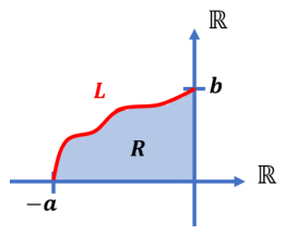
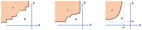
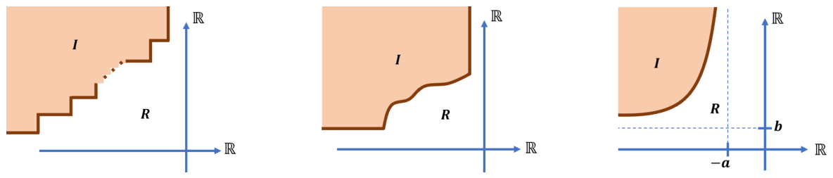
The central result of this study is Theorem 8, which demonstrates that the complement of a simply connected region forms an ideal of if and only if its boundary contains no strictly decreasing segments. This geometric criterion provides a clear and effective description of ideals, leading naturally to the classification of maximal, principal, and prime ideals in . Furthermore, every ideal in is shown to admit a representation as a union of translates of the bipolar set of the form . Such representations possess minimal generating sets M, although these generating sets need not be unique. The geometric nature of these ideals is further illustrated in Figure 27, which visually supports the findings presented in Theorems 5 and 6.
Figure 27.
Illustrations of the theorems: (left) Theorem 5, (right) Theorem 6.
We also establish that for any and any ideal , the translate is itself an ideal. Consequently, all regions identified in Theorem 4 through Corollary 1 remain ideals when translated by a vector , as shown in Figure 28 and Figure 29. In addition, Theorem 7 provides a sufficient condition for a region not to be an ideal, while Theorem 9 extends the characterization of ideals generated by arbitrary nonempty subsets . These results are further generalized to open ideals by considering the structure of the interior .
Figure 28.
The region I, obtained by a translation of the area shown in Figure 9.
Finally, we clarify the distinctions between ideals, quasi-ideals, and bi-ideals. In the commutative setting of , ideals and quasi-ideals are identical, while bi-ideals form a strictly larger class (see Figure 30). These relationships, illustrated through geometric examples, highlight the fundamental importance of a geometric approach in understanding the algebraic behavior of the bipolar semigroup.
Figure 30.
Illustrations of the results established in Proposition 2 (4) and Proposition 3.
Theorem 8, which defines ideality in terms of boundary monotonicity, extends naturally to the verification of policy consistency in cyber defense architectures. If the boundary of a defended region is non-decreasing, the corresponding security policy ensures that any increase in defensive capability never induces higher vulnerability exposure along its operational frontier. Conversely, the presence of a decreasing segment represents risk inversion, a situation where added protection paradoxically enlarges the attack surface. When interpreted operationally, this theorem becomes a formal validation rule for complex defense configurations: a structure is policy coherent if and only if its defense–vulnerability surface satisfies the monotonicity condition. This provides a mathematical analogue to configuration audits for layered systems, allowing automated detection of security regressions caused by conflicting controls or misaligned redundancies. From a practical standpoint, the implementations of these theorems could yield a class of analytic tools that transform semigroup structure into quantitative cybersecurity diagnostics. By embedding real network states into the bipolar plane, an organization could measure exposure as a geometric region, validate policies by testing for monotonic boundaries, and reconstruct forensic trajectories using the union of translates principle from Theorem 2. Together, these results provide a unified operational framework for reasoning about exposure, resilience, and compromise propagation—turning geometric invariance into a mechanism for auditing and enhancing adaptive security postures in real systems.
5. Discussions
The results obtained in this paper demonstrate the effectiveness of a geometric perspective in studying ideals within the semigroup . Instead of existing algebraic methods, we characterize ideality through boundary behavior rather than direct algebraic computation. This perspective is particularly useful for bipolar systems, as it relates geometric admissibility—characterized by the presence or absence of strictly decreasing boundary segments—as the principle governing invariant substructures. Consequently, this approach offers an intuitive, visual alternative to complex algebraic verification and paves the way for further exploration into the synergy between geometry and semigroup theory in fields such as ordered semigroups and module theory.
The geometric characterization developed in this paper suggests some natural directions for future work. One possible direction is to study ordered variants of the bipolar semigroup. The relation
defines a natural partial order on . This gives a setting in which ideals may be studied together with order-theoretic properties. For example, one may investigate order ideals and examine whether the boundary conditions obtained in this paper remain valid under this additional order structure.
Another possible direction is to consider fuzzy variants of bipolar ideals. In such a setting, an ideal-like subset may be replaced by a membership function
where represents the degree to which x belongs to the corresponding ideal-like region. A natural problem is to determine whether the boundary characterization in this paper has an analogue for such fuzzy ideals. These directions remain open and may provide further links between the algebraic structure of and its geometric representation.
One may also ask whether similar geometric ideas can be developed for related algebraic structures, such as semigroup actions or module-like constructions. Although these directions require additional definitions and lie beyond the scope of the present paper, the results obtained here indicate that boundary geometry may serve as a useful tool for characterizing invariant regions and admissible forms of algebraic expansion in more general algebraic settings.
Among the three proposed cybersecurity domains, attack surface quantification, policy consistency, and digital forensics, the bipolar semigroup model most directly enhances policy consistency through the application of Theorem 8. Because each policy can be represented as a boundary function , the monotonicity condition on f ensures that defensive investments preserve or improve overall protection. This transforms a quantitative geometric property into a compliance benchmark for secure design. Visualizing policy invariance as a topological constraint not only simplifies verification but also enables the detection of non obvious misconfigurations where added countermeasures unintentionally increase exposure. In this sense, the bipolar model provides a rigorous foundation for validating layered defense architectures via mathematical invariants rather than ad hoc checks. Nevertheless, attack surface formalization (via mapping to the bipolar state space) also exhibits strong potential for embodied metrics. Under the mapping , every network configuration can be represented as a point in the bipolar plane, and the ensemble of such points defines the effective attack surface . The introduction of the exposure functional yields a tractable scalar quantity for ranking configurations or thresholding acceptable risk. Incorporating this geometric view into existing frameworks such as attack tree metrics or vulnerability scoring [28] could bridge structural algebra with probabilistic risk modelling. This would align this theory with ongoing efforts to generalize security metrics in compositional and quantum inspired settings. Additionally, future research can expand on digital forensic applications by operationalizing Theorem 2. Representing the compromised region as allows each to be interpreted as a minimal intrusion vector, while the connecting paths trace the causal chain of lateral movement and escalation. Integrating this with current advances [29] would permit algebraic trace back analysis that is provably consistent with unclonable or quantum secured evidentiary models. Ultimately, uniting these directions could yield a multilevel framework where system states evolve geometrically, security policies are verified by boundary monotonicity, and forensic reconstructions emerge from minimal generating sets, thereby grounding cyber resilience, verification, and attribution within a single bipolar geometric formalism.
Finally, we distinguish this work from previous studies, such as [17], which primarily adopt an algebraic viewpoint. While [17] investigates ideal classes in bipolar semirings using internal algebraic operations and elementary real analysis (particularly the infimum), the present paper introduces a geometric framework based on boundary monotonicity. This provides an external geometric criterion for identifying invariant substructures beyond purely algebraic constraints. These conceptual and structural differences, summarized in Table 2, indicate that the present study offers a complementary geometric perspective with its own methodological characteristics and analytical tools.
Table 2.
A summary of differences between the present work and [17].
In summary, this work demonstrates that ideal structure in bipolar algebra can be effectively characterized through geometric boundary behavior, and that algebraic operations fundamentally influence geometric asymmetry. This perspective not only unifies algebraic and geometric viewpoints but also opens a pathway toward applying abstract semigroup theory in complex system modeling.
Remark 6.
so these vectors lie on the line . Also, , and similarly the corresponding vectors lie on . Hence, the lines and form the boundaries of a V-shape associated with the ideal generated by . Moreover, for any , we get
which is a sum of vectors on and . Therefore, every such product lies inside the V-shape region bounded by these two lines, see more details in [17].
We further explain the origin of the V-shaped pattern, which describes the shape of the ideal I in the semiring .
- Let . For any ,
Author Contributions
Conceptualization, K.L. and P.K.; methodology, K.L. and P.K.; writing—original draft preparation, K.L. and P.K.; writing—review and editing, K.L., R.M., D.M.C. and P.K. All authors have read and agreed to the published version of the manuscript.
Funding
This research received no external funding.
Data Availability Statement
No new data were created or analyzed in this study. Data sharing is not applicable to this article.
Acknowledgments
The authors would like to express their deepest gratitude to the reviewers for their careful reading, thoughtful comments, and valuable suggestions. Their insightful observations significantly improved the clarity, rigor, and overall quality of this manuscript. The authors also gratefully acknowledge Attawut Wongpradit and Thawit Hanvattanakul for their support.
Conflicts of Interest
The authors declare no conflicts of interest.
References
- Clifford, A.H. Semigroups without nilpotent ideals. Am. J. Math. 1949, 71, 834–844. [Google Scholar] [CrossRef] [Scilit]
- Reynolds, M.A.; Sullivan, R.P. The ideal structure of idempotent-generated transformation semigroups. Proc. Edinb. Math. Soc. 1985, 28, 319–331. [Google Scholar] [CrossRef] [Scilit]
- Honyam, P.; Sanwong, J. Semigroups of transformations with invariant set. J. Korean Math. Soc. 2011, 48, 289–300. [Google Scholar] [CrossRef] [Scilit]
- Honyam, P.; Sanwong, J. Semigroups of transformations with fixed sets. Quaest. Math. 2013, 36, 79–92. [Google Scholar] [CrossRef] [Scilit]
- Khachorncharoenkul, P.; Laipaporn, K.; Wananiyakul, S. Left almost seminearrings. Lobachevskii J. Math. 2020, 41, 349–361. [Google Scholar] [CrossRef] [Scilit]
- Senapati, T.; Jun, Y.B.; Iampan, A.; Chinram, R. Cubic intuitionistic structure applied to commutative ideals of BCK-algebras. Thai J. Math. 2022, 20, 877–887. Available online: https://thaijmath.com/index.php/thaijmath/article/view/1367 (accessed on 14 April 2024).
- Bussaban, L.; Changphas, T. On (m,n)-ideals and (m,n)-regular ordered semigroups. Songklanakarin J. Sci. Technol. 2016, 38, 199–206. [Google Scholar] [CrossRef] [Scilit]
- Awolola, J.A.; Ibrahim, M.A. A survey on fuzzy semigroups. Ratio Math. 2021, 40, 7–25. [Google Scholar] [CrossRef] [Scilit]
- Song, S.Z.; Kim, H.S.; Jun, Y.B. Ideal theory in semigroups based on intersectional soft sets. Sci. World J. 2014, 2014, 136424. [Google Scholar] [CrossRef] [Scilit]
- Vanishree, M.; Rajesh, N.; Rafi, N.; Bandaru, R. Ideal theory of semigroups based on (3,2)-fuzzy sets. J. Math. Comput. Sci. 2023, 28, 182–191. [Google Scholar] [CrossRef] [Scilit]
- Prasertpong, R.; Buada, S. Rough interior ideals and rough quasi-ideals in approximation spaces of semigroups under preorder and compatible relations. Suan Sunandha Sci. Technol. J. 2022, 8, 21–26. Available online: https://li02.tci-thaijo.org/index.php/ssstj/article/view/381 (accessed on 14 April 2024).
- Lekkoksung, S.; Davvaz, B.; Lekkoksung, N. An application of generalized fuzzy ideals in ordered semigroups. Eur. J. Pure Appl. Math. 2024, 17, 2962–2984. [Google Scholar] [CrossRef] [Scilit]
- Zhang, W.R. YinYang Bipolar Relativity: A Unifying Theory of Nature, Agents and Causality with Applications in Quantum Computing, Cognitive Informatics and Life Sciences; IGI Global Publishing: Hershey, PA, USA, 2011. [Google Scholar] [CrossRef] [Scilit]
- Zhang, W.R. Global realism with bipolar strings: From bell test to real-world causal-logical quantum gravity and brain-universe similarity for entangled machine thinking and imagination. Information 2024, 15, 456. [Google Scholar] [CrossRef] [Scilit]
- Almuhaimeed, A.; Alshehri, H. Bipolar fuzzy commutative ideals in BCK-algebras. Eur. J. Pure Appl. Math. 2024, 17, 1831–1841. [Google Scholar] [CrossRef] [Scilit]
- Varol, B.P.; Malkoc, H. Bipolar fuzzy supra topology via (Q-)neighborhood and its application in data mining process. Symmetry 2024, 16, 216. [Google Scholar] [CrossRef] [Scilit]
- Laipaporn, K.; Khachorncharoenkul, P. Ideals in the bipolar quantum linear algebra. Symmetry 2024, 16, 924. [Google Scholar] [CrossRef] [Scilit]
- Clifford, A.; Preston, G. The Algebraic Theory of Semigroups, Number 7, Part I; American Mathematical Society: Providence, RI, USA, 1961. [Google Scholar]
- Kapp, K.M. On bi-ideals and quasi-ideals in semigroups. Publ. Math. Debr. 1969, 16, 179–185. [Google Scholar] [CrossRef] [Scilit]
- Zhang, W.R. YinYang bipolar atom-An eastern road toward quantum gravity. J. Mod. Phys. 2012, 3, 1261–1271. [Google Scholar] [CrossRef]
- Munkres, J.R. Topology, 2nd ed.; Prentice Hall, Inc.: Hoboken, NJ, USA, 2000. [Google Scholar]
- Stewart, J. Calculus: Early Transcendentals, 7th ed.; Brooks/Cole, Cengage Learning: Boston, MA, USA, 2012. [Google Scholar]
- Schwarz, S. Prime ideals and maximal ideals in semigroups. Czechoslov. Math. J. 1969, 1, 72–79. Available online: http://dml.cz/dmlcz/100877 (accessed on 14 April 2024). [CrossRef] [Scilit]
- Bughio, K.; Cook, D.; Shah, A. Developing a novel ontology for cybersecurity in internet of medical things-enabled remote patient monitoring. Sensors 2024, 24, 2804. [Google Scholar] [CrossRef] [Scilit]
- Zhang, W.R. Bipolar quantum logic gates and quantum cellular combinatorics—A logical extension to quantum entanglement. J. Quantum Inf. Sci. 2013, 3, 93–105. [Google Scholar] [CrossRef]
- Manadhata, P.K.; Wing, J.M. An attack surface metric. IEEE Trans. Softw. Eng. 2011, 37, 371–386. [Google Scholar] [CrossRef] [Scilit]
- NIST. Engineering Trustworthy Secure Systems; Technical Report; NIST SP 800-160; U.S. Department of Commerce: Washington, DC, USA, 2016; Volume 1.
- Peterseim, B.; Lopuhaä-Zwakenberg, M. A unified compositional view of attack tree metrics. arXiv 2025, arXiv:2511.14717. [Google Scholar] [CrossRef] [Scilit]
- Goyal, V.; Raizes, J. Proofs of no intrusion. arXiv 2025, arXiv:2510.06432. [Google Scholar] [CrossRef] [Scilit]





Disclaimer/Publisher’s Note: The statements, opinions and data contained in all publications are solely those of the individual author(s) and contributor(s) and not of MDPI and/or the editor(s). MDPI and/or the editor(s) disclaim responsibility for any injury to people or property resulting from any ideas, methods, instructions or products referred to in the content. |
© 2026 by the authors. Licensee MDPI, Basel, Switzerland. This article is an open access article distributed under the terms and conditions of the Creative Commons Attribution (CC BY) license.