On Mixed Degenerate Gould–Hopper–Appell Polynomials: Structural Properties and Zero Distribution

Abstract

This article introduces and develops a comprehensive theory of the Mixed Degenerate Gould–Hopper–Appell Type Polynomials $MDGHA$-$TPs$, constructed by embedding an Appell factor into the framework of degenerate Gould–Hopper generating functions. Beginning with the generating function formulation, we derive explicit series representations, monomial-type operational identities, recurrence relations, and a determinantal form that encodes the algebraic structure of the family. Summation identities expressed via Stirling numbers of the first kind and addition-type formulas are established. A detailed numerical investigation of the zero distributions of these polynomials is then carried out, with graphical illustrations revealing symmetry patterns and geometric arrangements in the complex plane. Connections with classical sequences of Appell, Hermite, and Gould–Hopper are explored throughout. The article concludes with remarks on open problems including the orthogonality of the $MDGHA$-$TPs$ with respect to suitable weight functions, the asymptotic behaviour of their zeros as the degree tends to infinity, and potential applications to boundary-value problems in heat diffusion, perturbation expansions in quantum mechanics, and signal processing in non-homogeneous media.

1. Introduction

1.1. Motivation

The introduction of the Mixed Degenerate Gould–Hopper–Appell-Type Polynomials ($MDGHA$-$TPs$) is motivated by three independent lines of inquiry that together justify the triple unification as the minimal combination capturing all three phenomena simultaneously.

First, the Carlitz degenerate polynomial programme replaces the classical exponential $e^{x\tau }$ by the binomial ${(1+\lambda \tau )}^{x/\lambda }$, introducing falling-factorial coefficients and Stirling numbers of the first kind into all convolution identities, with connections to p-adic analysis and finite-field arithmetic. Second, the Gould–Hopper kernel $exp\left(x_2{\tau }^m\right)$ of order m models higher-order diffusion equations ${\partial }_{t}u=c{\partial }_x^{m}u$ and anharmonic-oscillator Hamiltonians in mathematical physics; its interaction with the degenerate exponential via the scaling ratio $\mu =\lambda /log(1+\lambda )$ is intrinsic to the mixed family and produces structural features absent in either factor alone. Third, the Appell factor $g\left(\tau \right)$ encodes number-theoretic structures (Bernoulli, Euler, Genocchi polynomials) whose Stirling-number expansion interacts non-trivially with the higher-order exponential, producing the summation identities of Theorem 6 that are not recoverable from any pairwise combination. The $MDGHA$-$TPs$ constitute the minimal hybrid family in which all three interactions are simultaneously present and structurally operative.

Special polynomial sequences sit at a productive junction between pure mathematics and the physical sciences. Families such as the Bernoulli, Euler, Hermite, Laguerre, and Legendre polynomials emerge as solutions to classical differential equations governing quantum mechanical systems, heat diffusion, electrostatics, and function approximation. Their orthogonality relations, three-term recurrences, and generating function representations have been studied for well over a century, and extensions of these families to degenerate, multivariate, or hybrid settings continue to attract sustained research interest, uncovering algebraic interconnections that were invisible in the classical setting [1,2,3,4,5,6,7,8,9,10,11,12].

Among these classical families, the Hermite polynomials introduced by Charles Hermite in the 19th century [13] are arguably the most pervasive. Their exponential generating function is

$$e^{-{\tau }^2+2x_1\tau }={\displaystyle \sum _{n=0}^{\infty }}{\mathcal{H}}_n\left(x_1\right){\displaystyle \frac{{\tau }^n}{n!}},$$

(1)

and they arise as eigenstates of the quantum harmonic oscillator and as the weight functions for Gauss–Hermite quadrature. The natural two-variable extension, due to Appell and Kampé de Fériet [14], is given by the explicit sum

$${\mathcal{H}}_n(x_1,x_2)=n!{\displaystyle \sum _{r=0}^{\lfloor n/2\rfloor }}{\displaystyle \frac{x_2^r{x}_1^{n-2r}}{r!(n-2r)!}},$$

(2)

The two-variable Hermite polynomials ${\mathcal{H}}_n(x_1,x_2)$ defined by the explicit sum (2) arise naturally as the coefficient sequence of the exponential generating function. To see this, one expands $e^{x_1\tau +x_2{\tau }^2}=e^{x_1\tau }·e^{x_2{\tau }^2}$, substituting the Taylor series $e^{x_1\tau }={\sum }_{j=0}^{\infty }{x}_1^j{\tau }^j/j!$ and $e^{x_2{\tau }^2}={\sum }_{r=0}^{\infty }{x}_2^r{\tau }^{2r}/r!$, and collecting the coefficient of ${\tau }^n/n!$ via the Cauchy product. This yields precisely the double sum in (2), confirming that (2) and (3) define the same family.

Which corresponds to the generating relation

$${\displaystyle \sum _{n=0}^{\infty }}{\mathcal{H}}_n(x_1,x_2){\displaystyle \frac{{\tau }^n}{n!}}=e^{x_1\tau +x_2{\tau }^2}.$$

(3)

A natural higher-order counterpart is the Gould–Hopper family ${\mathcal{H}}_n^{\left(m\right)}\left(x_1\right)$ [15], defined through the generating relation

$$exp(x_1\tau +{\tau }^m)={\displaystyle \sum _{n=0}^{\infty }}{\mathcal{H}}_n^{\left(m\right)}\left(x_1\right){\displaystyle \frac{{\tau }^n}{n!}},$$

(4)

with series representation

$${\mathcal{H}}_n^{\left(m\right)}\left(x_1\right)=n!{\displaystyle \sum _{r=0}^{\lfloor n/m\rfloor }}{\displaystyle \frac{x_1^{n-mr}}{(n-mr)!r!}},$$

(5)

which recovers the classical Hermite family when $m=2$.

A parallel development concerns the Appell sequences [16]. A sequence ${\left\{A_n\left(x\right)\right\}}_{n\ge 0}$ is an Appell sequence when it satisfies the differentiation rule

$${\displaystyle \frac{d}{dx}}{A}_n\left(x\right)=n{A}_n(x-1),n\ge 1,$$

(6)

or, what amounts to the same thing, when its generating function takes the form

$$g\left(\tau \right)e^{x\tau }={\displaystyle \sum _{n=0}^{\infty }}{A}_n\left(x\right){\displaystyle \frac{{\tau }^n}{n!}},$$

(7)

where

$$g\left(\tau \right)={\displaystyle \sum _{n=0}^{\infty }}{a}_n{\displaystyle \frac{{\tau }^n}{n!}},g\left(0\right)=a_0\ne 0,$$

(8)

so that $g\left(\tau \right)$ is an invertible formal power series, ensuring the well-definedness of the Appell sequence and, as noted in the proof of Theorem 9, the unique solvability of the Costabile inversion procedure. The Bernoulli polynomials ($g\left(\tau \right)=\tau /(e^{\tau }-1)$), Euler polynomials ($g\left(\tau \right)=2/(e^{\tau }+1)$), and Genocchi polynomials are the canonical representatives of this class, and their number-theoretic properties have been studied extensively [6,17,18].

A systematic deformation of all these families was initiated by Carlitz [19], who replaced the classical exponential $e^{x\tau }$ by the degenerate counterpart ${(1+\lambda \tau )}^{x/\lambda }$. This substitution defines the degenerate exponential

$${(1+\lambda \tau )}^{x/\lambda }={\displaystyle \sum _{n=0}^{\infty }}{\mathcal{DE}}_n(x;\lambda ){\displaystyle \frac{{\tau }^n}{n!}},$$

(9)

The degenerate exponential differs from the classical exponential in that it replaces the additive exponent $x\tau$ by the multiplicative binomial structure ${(1+\lambda \tau )}^{x/\lambda }$; when expanded, it introduces falling-factorial coefficients that give rise to Stirling numbers of the first kind, making $\lambda$ a structural parameter rather than merely a scaling factor. and the parameter $\lambda$ controls the deformation: as $\lambda \to 0$ one recovers $e^{x\tau }$ and the classical polynomials emerge as limiting cases. The degenerate programme has since been carried through for the Bernoulli, Euler, Stirling, Hermite, and Apostol-type families, producing a body of results with connections to p-adic analysis, umbral calculus, and combinatorics [17,19,20,21]. Recent work by the present authors [7] has established quasi-monomial frameworks and determinant representations for several degenerate hybrid families, motivating the broader construction undertaken in this paper.

Combining the Appell factor with the Gould–Hopper exponential kernel yields the Gould–Hopper–Appell polynomials [5,6], defined by

$$g\left(\tau \right)exp(x_1\tau +x_2{\tau }^m)={\displaystyle \sum _{n=0}^{\infty }}{\mathcal{GHA}}_n^{\left[m\right]}(x_1,x_2){\displaystyle \frac{{\tau }^n}{n!}}.$$

(10)

This hybrid generating function simultaneously encodes Appell-type features and higher-order Hermite structure, and it is the starting point for the present generalisation.

The specific unification of these three constituents—the Appell factor $g\left(\tau \right)$, the Carlitz degenerate exponential ${(1+\lambda \tau )}^{x_1/\lambda }$, and the Gould–Hopper kernel $exp\left(x_2{\tau }^m\right)$—is not merely formal but is motivated by three independent lines of application. First, the Appell factor $g\left(\tau \right)$ encodes number-theoretic and combinatorial structures (Bernoulli, Euler, Genocchi polynomials) whose Stirling-number expansion interacts non-trivially with the higher-order exponential; this interaction produces the Stirling-number summation identities of Theorem 6, which are not recoverable from any pairwise combination. Second, the degenerate exponential provides a one-parameter ($\lambda$) regularisation that simultaneously recovers the classical limit as $\lambda \to 0$ and connects to p-adic and finite-field analogues; the coupling of $\lambda$ with the Gould–Hopper index m via the scaling ratio $\mu =\lambda /log(1+\lambda )$ in the quasi-monomial operators of Theorem 4 is intrinsic to the mixed family and not a feature of either factor alone. Third, the Gould–Hopper kernel of order m models higher-order diffusion and anharmonic-oscillator equations in mathematical physics; grafting the Appell and degenerate structures onto this kernel produces a family suitable for studying discretised or deformed versions of such equations. Together, these three motivations distinguish the $MDGHA$-$TPs$ from other products of generating functions and justify the triple unification as the minimal combination capturing all three phenomena simultaneously.

Motivated by recent results in degenerate polynomial theory [12,17,18,22] and the quasi-monomial formalism of Dattoli and colleagues [23,24], we introduce the Mixed Degenerate Gould–Hopper–Appell-Type Polynomials ($MDGHA$-$TPs$). This family incorporates the degenerate exponential (9), the Gould–Hopper kernel of order m, and an Appell factor $g\left(\tau \right)$ within a unified two-variable framework. Each of the three constituent families is a special case, and their interaction brings out certain characteristics of structure that would not have been apparent from the analysis of any one of the constituent families alone.

The quasi-monomial approach, developed by Steffensen [25] and greatly improved by Dattoli [23,24], forms the principal operational approach used in the following sections. The family of polynomials ${\left\{{\mathcal{P}}_n\left(x\right)\right\}}_{n\ge 0}$ is said to be quasi-monomial under the action of operators $\widehat{\mathcal{M}}$ and $\widehat{\mathcal{D}}$ when

$${\mathcal{P}}_{n+1}\left(x\right)=\widehat{\mathcal{M}}{\mathcal{P}}_n\left(x\right),n{\mathcal{P}}_{n-1}\left(x\right)=\widehat{\mathcal{D}}{\mathcal{P}}_n\left(x\right),$$

(11)

with the commutation relation

$$[\widehat{\mathcal{D}},\widehat{\mathcal{M}}]=\widehat{\mathcal{D}}\widehat{\mathcal{M}}-\widehat{\mathcal{M}}\widehat{\mathcal{D}}=\widehat{1},$$

(12)

Here $\widehat{1}$ denotes the identity operator on the space of formal power series, so the commutation relation $[\widehat{\mathcal{D}},\widehat{\mathcal{M}}]=\widehat{1}$ states that $\widehat{\mathcal{D}}\widehat{\mathcal{M}}-\widehat{\mathcal{M}}\widehat{\mathcal{D}}$ acts as the identity; this is precisely the Weyl–Heisenberg canonical commutation relation, familiar from quantum mechanics where $\widehat{\mathcal{M}}$ and $\widehat{\mathcal{D}}$ play the roles of the creation and annihilation operators, respectively. which places the operators within a Weyl–Heisenberg algebra. Three consequences follow directly.

(i)

The family satisfies the differential equation

$$\widehat{\mathcal{M}}\widehat{\mathcal{D}}{\mathcal{P}}_n\left(x\right)=n{\mathcal{P}}_n\left(x\right).$$

(13)

(ii)

Every member can be expressed operationally as

$${\mathcal{P}}_n\left(x\right)={\widehat{\mathcal{M}}}^n\left\{1\right\},{\mathcal{P}}_0\left(x\right)=1.$$

(14)

(iii)

The exponential generating function is recoverable from the multiplicative operator via

$$e^{\tau \widehat{\mathcal{M}}}\left\{1\right\}={\displaystyle \sum _{n=0}^{\infty }}{\mathcal{P}}_n\left(x\right){\displaystyle \frac{{\tau }^n}{n!}},\left|\tau \right|<\infty .$$

(15)

Integral representations and non-standard generating function techniques for multi-dimensional Chebyshev and Hermite families were developed in [26,27]; those methods complement and partially motivate the quasi-monomial treatment adopted here.

Remark 1

(Sheffer-type sequences). Every Appell sequence $\left\{A_n\left(x\right)\right\}$ is a Sheffer sequence for the pair $\left(g\right(\tau ),\tau )$ in the sense of umbral calculus. The $MDGHA$-$TPs$ inherit this Sheffer structure through their Appell factor $g\left(\tau \right)$, but are not themselves standard Sheffer sequences because the derivative operator ${\widehat{\mathcal{D}}}_{\mathcal{A}}=\mu {\partial }_{x_1}$ involves the degenerate scaling $\mu =\lambda /log(1+\lambda )\ne 1$ for $\lambda \ne 0$. They are therefore degenerate Sheffer sequences in a sense currently being formalised in the literature. The Rodrigues-type operational identity takes the form

$${}_{\mathcal{DE}}\mathcal{A}_n^{\left[m\right]}(x_1,x_2;\lambda )=g{\left({\mu }^{-1}{\partial }_{x_1}\right)}^{-1}exp\left(x_2{\mu }^{-m}{\partial }_{x_1}^m\right)x_1^n;$$

a classical Rodrigues formula involving a weight function and n-th derivative remains an open problem for the $MDGHA$-$TPs$.

Special polynomial families serve as a meeting ground for combinatorics, analysis, and mathematical physics, and the present work introduces the Mixed Degenerate Gould–Hopper–Appell-Type Polynomials ($MDGHA$-$TPs$), defined by the generating function $g\left(\tau \right){(1+\lambda \tau )}^{x_1/\lambda }exp\left(x_2{\tau }^m\right)$, uniting the Appell factor $g\left(\tau \right)$, the Carlitz degenerate exponential ${(1+\lambda \tau )}^{x_1/\lambda }$, and the Gould–Hopper kernel $exp\left(x_2{\tau }^m\right)$ within a single two-variable framework whose three-way interaction produces structural phenomena invisible in any pairwise case. The quasi-monomial derivative operator of Theorem 4 reveals this concretely: the degenerate scaling ratio $\mu =\lambda /log(1+\lambda )$ couples with the Gould–Hopper index m via ${\mu }^{m-2}{\partial }_{x_1}^{m-1}$, a feature intrinsic to the mixed family that collapses to known results only in separate degenerate or classical limits. The summation identities of Theorem 6 exhibit a further genuine interaction, as the expansion of ${(1+\lambda \tau )}^{x_1/\lambda }$ in powers of $log(1+\lambda \tau )$ forces Stirling numbers of the first kind into the convolution with the Gould–Hopper exponential, where they play a structural rather than a merely bookkeeping role. The determinantal form of Theorem 9, derived via the Costabile inversion procedure, packages these interactions into a closed-form expression making the recursive dependence among family members both explicit and computationally tractable. The zero distribution of the Bernoulli subfamily ${}_{\mathcal{DE}}\mathcal{B}_n^{\left[4\right]}(x_1,35;1)$, investigated analytically and numerically in Section 5, provides the most telling evidence of the family’s richness. Proposition 1 establishes that the reflection symmetry $x_1\leftrightarrow 1-x_1$, a hallmark of the classical Bernoulli polynomials, survives intact into the degenerate Gould–Hopper setting for purely structural reasons. A guaranteed zero at $x_1=\frac{1}{2}$ for every odd degree follows directly from this symmetry, and its persistence across all tested parameter values confirms it as a robust feature rather than an artifact of the choices $m=4$, $x_2=35$, $\lambda =1$. Taken together, these results establish that the $MDGHA$-$TPs$ constitute not a formal generalization alone but a family with genuine structure meriting further investigation from both theoretical and applied perspectives.

1.2. Highlights of the Paper

The five principal contributions of this article are as follows.

1.

Explicit series representations (Theorem 1): The $MDGHA$-$TPs$ are expressed as a finite convolution of the underlying degenerate Appell polynomials ${\mathcal{A}}_{n-mk}(x_1;\lambda )$ with powers of $x_2$, providing a computationally accessible closed form.

2.

Quasi-monomial structure (Theorems 4 and 5): Multiplicative and derivative operators ${\widehat{\mathcal{M}}}_{\mathcal{A}}$ and ${\widehat{\mathcal{D}}}_{\mathcal{A}}$ are identified, and the associated partial differential equation of order m in ${\partial }_{x_1}$ is derived, characterising the $MDGHA$-$TPs$ as eigenfunctions of ${\widehat{\mathcal{M}}}_{\mathcal{A}}{\widehat{\mathcal{D}}}_{\mathcal{A}}$ with eigenvalue n.

3.

Summation and addition formulae (Theorem 6): Identities involving Stirling numbers of the first kind connect the $MDGHA$-$TPs$ to the degenerate Appell polynomials; bivariate addition formulas and a convolution identity are also established.

4.

Determinantal representation (Theorem 9): The family is expressed via a lower Hessenberg determinant, providing an explicit and recursion-free representation of every member.

5.

Zero distribution results (Proposition 1): For the Bernoulli subfamily, conjugate pairing, quadruple symmetry for even degree, and a guaranteed zero at $x_1=\frac{1}{2}$ for odd degree are established analytically and confirmed numerically.

1.3. Implications of the Main Findings

The results of this article carry several implications for the structural theory of the $MDGHA$-$TPs$ and for their potential applications.

The quasi-monomial structure of Theorems 4 and 5 places the $MDGHA$-$TPs$ within the Weyl–Heisenberg operator algebra, enabling systematic operator-theoretic analysis. The differential equation of Theorem 5 is of order m in ${\partial }_{x_1}$, connecting the family to spectral theory for higher-order degenerate differential operators. The Stirling-number identities of Theorem 6 provide explicit bridges to p-adic analysis and to the combinatorial theory of degenerate polynomial families. The lower Hessenberg determinantal form of Theorem 9 is computationally efficient and makes the recursive structure among family members transparent. Finally, the analytically proved zero-symmetry properties of Proposition 1 show that the Appell factor influences the zero distribution in a quantitatively controlled and predictable way, with implications for approximation theory, potential theory, and the study of zeros of generating functions in mathematical physics.

The paper proceeds in the following manner. In Section 2, the $MDGHA$-$TPs$ are defined through their generating functions, and their main properties such as series representations and differential recurrence relations are derived. In Section 3, the quasi-monomiality property of these polynomials is obtained, along with their differential equation, summation formulas using the Stirling numbers of the first kind, and addition formulas. Section 4 contains an exploratory study of the zeros of these polynomials, which includes numerical examples. Section 5 ends with concluding remarks and some open problems.

2. Preliminaries

This section collects the foundational definitions, generating functions, and operator framework that underlie the construction of the $MDGHA$-$TPs$. All variables satisfy $x_1,x_2\in \mathbb{R}$, $\tau \in \mathbb{C}$, $\lambda \in \mathbb{R}\setminus \left\{0\right\}$, and $m\in \mathbb{N}$ throughout, unless otherwise stated.

3. Mixed Degenerate Gould–Hopper–Appell-Type Polynomials

The Appell polynomial factor $g\left(\tau \right)$, when combined with the degenerate exponential kernel and the Gould–Hopper higher-order structure, produces a rich and flexible polynomial family. We now introduce the central object of this study.

Definition 1.

The Mixed Degenerate Gould–Hopper–Appell-Type Polynomials ($MDGHA$-$TPs$), denoted by ${}_{\mathcal{DE}}\mathcal{A}_n^{\left[m\right]}(x_1,x_2;\lambda )$, where $x_1,x_2\in \mathbb{R}$, $\lambda \in \mathbb{R}\setminus \left\{0\right\}$, and $m\in \mathbb{N}$, are defined through the generating function

$${\displaystyle \sum _{n=0}^{\infty }}{}_{\mathcal{DE}}\mathcal{A}_n^{\left[m\right]}(x_1,x_2;\lambda ){\displaystyle \frac{{\tau }^n}{n!}}=g\left(\tau \right){(1+\lambda \tau )}^{{\displaystyle \frac{x_1}{\lambda }}}exp\left(x_2{\tau }^m\right),$$

(16)

where $g\left(\tau \right)={\sum }_{k=0}^{\infty }{a}_k{\tau }^k/k!$ is a formal power series with $g\left(0\right)=a_0\ne 0$. The generating function converges for $\left|\lambda \tau \right|<1$ (as required by the binomial series ${(1+\lambda \tau )}^{x_1/\lambda }$) and for $\left|\tau \right|$ sufficiently small relative to $|x_2{|}^{1/m}$ (as required by the Gould–Hopper exponential). For $g\left(\tau \right)$ analytic with radius of convergence $R_g>0$, the overall radius of convergence is $min(1/|\lambda |,R_g)$.

Remark 2.

The three-factor structure in Equation (16) deserves emphasis.

• The Appell factor $g\left(\tau \right)$ encodes the specific subfamily under study. Setting $g\left(\tau \right)=1$ recovers the mixed degenerate Gould–Hopper-type polynomials studied in [7]. For $g\left(\tau \right)=\tau /(e^{\tau }-1)$ one obtains a Bernoulli-type hybrid, and for $g\left(\tau \right)=2/(e^{\tau }+1)$ an Euler-type hybrid.
• The degenerate factor ${(1+\lambda \tau )}^{{\displaystyle \frac{x_1}{\lambda }}}\to e^{x_1\tau }$ as $\lambda \to 0$, recovering the classical Gould–Hopper–Appell family (10).
• For $m=2$ and $\lambda \to 0$, Equation (16) reduces to the generating function of the two-variable Hermite–Appell polynomials.
• The $MDGHA$-$TPs$ therefore sit at the apex of a three-fold generalisation hierarchy: they reduce to the Gould–Hopper–Appell polynomials as $\lambda \to 0$ (item above), to the degenerate Appell polynomials when $x_2=0$ (Theorem 3), and to the degenerate Gould–Hopper polynomials when $g\left(\tau \right)=1$.

We denote the full generating function on the right-hand side of Equation (16) by

$$\mathcal{F}(\tau ,x_1,x_2;\lambda )=g\left(\tau \right){(1+\lambda \tau )}^{{\displaystyle \frac{x_1}{\lambda }}}exp\left(x_2{\tau }^m\right).$$

(17)

A direct computation shows that $\mathcal{F}$ satisfies the first-order differential equation

$${\displaystyle \frac{\partial }{\partial \tau }}\mathcal{F}-\left({\displaystyle \frac{g^{\prime }\left(\tau \right)}{g\left(\tau \right)}}+{\displaystyle \frac{log(1+\lambda \tau )}{\lambda }}·{\displaystyle \frac{x_1}{\tau }}+m{x}_2{\tau }^{m-1}\right)\mathcal{F}=0,$$

(18)

from which, upon equating coefficients of ${\tau }^n$, one derives the recurrence relation

$$\begin{array}{c}{}_{\mathcal{DE}}\mathcal{A}_{n+1}^{\left[m\right]}(x_1,x_2;\lambda )={\displaystyle \sum _{k=0}^n}\left({\displaystyle \genfrac{}{}{0pt}{}{n}{k}}\right)a_{n-k+1}{}_{\mathcal{DE}}\mathcal{A}_k^{\left[m\right]}(x_1,x_2;\lambda )\hfill \\ +{\displaystyle \frac{log(1+\lambda )}{\lambda }}{x}_1{}_{\mathcal{DE}}\mathcal{A}_n^{\left[m\right]}(x_1,x_2;\lambda )+m{x}_{2}n(n-1)\cdots (n-m+2){}_{\mathcal{DE}}\mathcal{A}_{n-m+1}^{\left[m\right]}(x_1,x_2;\lambda ),\hfill \end{array}$$

(19)

valid for $n\ge m-1$. This recurrence combines three contributions: the Appell convolution term ${\sum }_k\left({\displaystyle \genfrac{}{}{0pt}{}{n}{k}}\right)a_{n-k+1}(\cdots )$, the degenerate-exponential term proportional to $x_1$, and the Gould–Hopper term proportional to $x_2$.

Differentiating Equation (17) with respect to $x_1$ yields

$${\displaystyle \frac{\partial }{\partial x_1}}\mathcal{F}(\tau ,x_1,x_2;\lambda )-{\displaystyle \frac{log(1+\lambda \tau )}{\lambda \tau }}·\tau \mathcal{F}(\tau ,x_1,x_2;\lambda )=0,$$

(20)

and comparison of coefficients of ${\displaystyle \frac{{\tau }^n}{n!}}$ on both sides produces the differential recurrence

$${\displaystyle \frac{\partial }{\partial x_1}}{}_{\mathcal{DE}}\mathcal{A}_n^{\left[m\right]}(x_1,x_2;\lambda )=n{\displaystyle \frac{log(1+\lambda )}{\lambda }}{}_{\mathcal{DE}}\mathcal{A}_{n-1}^{\left[m\right]}(x_1,x_2;\lambda ),n\ge 1.$$

(21)

Similarly, differentiating Equation (17) with respect to $x_2$ gives

$${\displaystyle \frac{\partial }{\partial x_2}}{}_{\mathcal{DE}}\mathcal{A}_n^{\left[m\right]}(x_1,x_2;\lambda )=n(n-1)\cdots (n-m+1){}_{\mathcal{DE}}\mathcal{A}_{n-m}^{\left[m\right]}(x_1,x_2;\lambda ),n\ge m.$$

(22)

Eliminating intermediate terms from Equations (19)–(22), one arrives at the identity

$${}_{\mathcal{DE}}\mathcal{A}_{n+1}^{\left[m\right]}={\displaystyle \frac{log(1+\lambda )}{\lambda }}{x}_1{}_{\mathcal{DE}}\mathcal{A}_n^{\left[m\right]}+{\displaystyle \frac{m{x}_2}{\lambda }}log(1+\lambda ){\displaystyle \frac{\partial }{\partial x_1}}{}_{\mathcal{DE}}\mathcal{A}_n^{\left[m\right]}+m{x}_2{\displaystyle \frac{\partial }{\partial x_2}}{}_{\mathcal{DE}}\mathcal{A}_n^{\left[m\right]}+{\displaystyle \sum _{k=0}^n}\left({\displaystyle \genfrac{}{}{0pt}{}{n}{k}}\right)a_{n-k+1}{}_{\mathcal{DE}}\mathcal{A}_k^{\left[m\right]}.$$

(23)

Differentiating Equation (23) with respect to $x_1$ and applying Equation (21) yields the mixed partial differential identity

$$\begin{array}{c}m{x}_2{\displaystyle \frac{{\partial }^2}{\partial x_1\partial x_2}}{}_{\mathcal{DE}}\mathcal{A}_n^{\left[m\right]}+{\displaystyle \frac{m{x}_2}{\lambda }}log(1+\lambda ){\displaystyle \frac{{\partial }^2}{\partial x_1^2}}{}_{\mathcal{DE}}\mathcal{A}_n^{\left[m\right]}+{\displaystyle \frac{log(1+\lambda )}{\lambda }}(x_1+n){}_{\mathcal{DE}}\mathcal{A}_n^{\left[m\right]}\hfill \\ \hfill +{\displaystyle \sum _{k=0}^n}\left({\displaystyle \genfrac{}{}{0pt}{}{n}{k}}\right)a_{n-k+1}{\displaystyle \frac{\partial }{\partial x_1}}{}_{\mathcal{DE}}\mathcal{A}_k^{\left[m\right]}=0,n\ge 0.\end{array}$$

(24)

We now derive the explicit series form of the $MDGHA$-$TPs$.

Theorem 1.

The $MDGHA$-$TPs$, denoted by ${}_{\mathcal{DE}}\mathcal{A}_n^{\left[m\right]}(x_1,x_2;\lambda )$, with $x_1,x_2\in \mathbb{R}$, $\lambda \in \mathbb{R}\setminus \left\{0\right\}$, $m\in \mathbb{N}$, admit the explicit representation

$${}_{\mathcal{DE}}\mathcal{A}_n^{\left[m\right]}(x_1,x_2;\lambda )=n!{\displaystyle \sum _{k=0}^{\lfloor n/m\rfloor }}{\displaystyle \frac{x_2^k}{k!}}{\displaystyle \frac{{\mathcal{A}}_{n-mk}(x_1;\lambda )}{(n-mk)!}},$$

(25)

where ${\mathcal{A}}_j(x_1;\lambda )$ denotes the j-th degenerate Appell polynomial defined through

$$g\left(\tau \right){(1+\lambda \tau )}^{{\displaystyle \frac{x_1}{\lambda }}}={\displaystyle \sum _{j=0}^{\infty }}{\mathcal{A}}_j(x_1;\lambda ){\displaystyle \frac{{\tau }^j}{j!}}.$$

(26)

Equivalently,

$${}_{\mathcal{DE}}\mathcal{A}_n^{\left[m\right]}(x_1,x_2;\lambda )=n!{\displaystyle \sum _{k=0}^{\lfloor n/m\rfloor }}\left({\displaystyle \genfrac{}{}{0pt}{}{n}{mk}}\right){\displaystyle \frac{\left(mk\right)!}{k!}}{\displaystyle \frac{{\mathcal{A}}_{n-mk}(x_1;\lambda )}{n!}}{x}_2^k.$$

(27)

Proof. 

From the definition (16), we write

$${\displaystyle \sum _{n=0}^{\infty }}{}_{\mathcal{DE}}\mathcal{A}_n^{\left[m\right]}(x_1,x_2;\lambda ){\displaystyle \frac{{\tau }^n}{n!}}=\left({\displaystyle \sum _{j=0}^{\infty }}{\mathcal{A}}_j(x_1;\lambda ){\displaystyle \frac{{\tau }^j}{j!}}\right)\left({\displaystyle \sum _{k=0}^{\infty }}{\displaystyle \frac{x_2^k}{k!}}{\tau }^{mk}\right),$$

(28)

where the first factor on the right is the generating function of the degenerate Appell polynomials ${\mathcal{A}}_j(x_1;\lambda )$ given by Equation (26), and the second factor is the Taylor expansion of $exp\left(x_2{\tau }^m\right)$. Applying the Cauchy product rule to the right-hand side of Equation (28), we obtain

$${\displaystyle \sum _{n=0}^{\infty }}{}_{\mathcal{DE}}\mathcal{A}_n^{\left[m\right]}(x_1,x_2;\lambda ){\displaystyle \frac{{\tau }^n}{n!}}={\displaystyle \sum _{n=0}^{\infty }}{\displaystyle \sum _{k=0}^{\lfloor n/m\rfloor }}{\displaystyle \frac{{\mathcal{A}}_{n-mk}(x_1;\lambda )}{(n-mk)!}}·{\displaystyle \frac{x_2^k}{k!}}{\tau }^n.$$

(29)

Comparing the coefficients of ${\displaystyle \frac{{\tau }^n}{n!}}$ on both sides of Equation (29) establishes Equation (25), and rewriting in terms of binomial coefficients yields Equation (27).    □

Theorem 2.

For $x_1=0$ and every integer $n\ge 0$, the $MDGHA$-$TPs$ satisfy

$${}_{\mathcal{DE}}\mathcal{A}_n^{\left[m\right]}(0,x_2;\lambda )=\left\{\begin{array}{cc}{\displaystyle \frac{n!}{(n/m)!}}{a}_0·x_2^{n/m},\hfill & \mathit{if}m\mid n,\hfill \\ {\displaystyle n!{\displaystyle \sum _{k=0}^{\lfloor n/m\rfloor }}{\displaystyle \frac{x_2^k}{k!}}·{\displaystyle \frac{{\mathcal{A}}_{n-mk}(0;\lambda )}{(n-mk)!}},}\hfill & \mathit{if}m\nmid n,\hfill \end{array}\right.$$

(30)

where ${\mathcal{A}}_j(0;\lambda )$ are the degenerate Appell numbers.

Proof. 

Setting $x_1=0$ in the generating function Equation (16) gives

$${\displaystyle \sum _{n=0}^{\infty }}{}_{\mathcal{DE}}\mathcal{A}_n^{\left[m\right]}(0,x_2;\lambda ){\displaystyle \frac{{\tau }^n}{n!}}=g\left(\tau \right){(1+\lambda \tau )}^{0}exp\left(x_2{\tau }^m\right)=g\left(\tau \right)exp\left(x_2{\tau }^m\right).$$

(31)

Expanding $exp\left(x_2{\tau }^m\right)={\sum }_{k=0}^{\infty }{x}_2^k{\tau }^{mk}/k!$ and $g\left(\tau \right)={\sum }_{j=0}^{\infty }{a}_j{\tau }^j/j!$, the Cauchy product yields

$${\displaystyle \sum _{n=0}^{\infty }}{}_{\mathcal{DE}}\mathcal{A}_n^{\left[m\right]}(0,x_2;\lambda ){\displaystyle \frac{{\tau }^n}{n!}}={\displaystyle \sum _{n=0}^{\infty }}{\displaystyle \sum _{k=0}^{\lfloor n/m\rfloor }}{\displaystyle \frac{a_{n-mk}}{(n-mk)!}}·{\displaystyle \frac{x_2^k}{k!}}{\tau }^n.$$

(32)

Comparing coefficients of ${\displaystyle \frac{{\tau }^n}{n!}}$ and noting that ${\mathcal{A}}_j(0;\lambda )=a_j$ (the Appell numbers), one obtains the general expression. In the special case $m\mid n$, the dominant term $k=n/m$ contributes $a_0·x_2^{n/m}/(n/m)!$ multiplied by $n!$, while the remaining terms vanish only when $g\left(\tau \right)$ reduces to a constant, giving Equation (30).    □

Theorem 3.

For $x_2=0$ and every integer $n\ge 0$,

$${}_{\mathcal{DE}}\mathcal{A}_n^{\left[m\right]}(x_1,0;\lambda )={\mathcal{A}}_n(x_1;\lambda ),$$

(33)

that is, the $MDGHA$-$TPs$ reduce to the degenerate Appell polynomials when $x_2=0$.

Proof. 

Setting $x_2=0$ in Equation (16),

$${\displaystyle \sum _{n=0}^{\infty }}{}_{\mathcal{DE}}\mathcal{A}_n^{\left[m\right]}(x_1,0;\lambda ){\displaystyle \frac{{\tau }^n}{n!}}=g\left(\tau \right){(1+\lambda \tau )}^{{\displaystyle \frac{x_1}{\lambda }}}exp\left(0\right)=g\left(\tau \right){(1+\lambda \tau )}^{{\displaystyle \frac{x_1}{\lambda }}}.$$

(34)

By definition, in Equation (26), the right-hand side generates ${\mathcal{A}}_n(x_1;\lambda )$, so comparison of coefficients of ${\displaystyle \frac{{\tau }^n}{n!}}$ gives Equation (33). Alternatively, in the explicit formula Equation (25), setting $x_2=0$ annihilates every term except $k=0$, leaving ${}_{\mathcal{DE}}\mathcal{A}_n^{\left[m\right]}(x_1,0;\lambda )={\mathcal{A}}_n(x_1;\lambda )$.    □

The result of Theorem 3 has a clear structural interpretation: the Gould–Hopper kernel $exp\left(x_2{\tau }^m\right)$ is responsible for introducing the higher-order (m-th degree) interactions encoded in the $x_2$-variable. When $x_2=0$ this kernel becomes trivial, and the generating function $g\left(\tau \right){(1+\lambda \tau )}^{x_1/\lambda }$ retains only the interplay between the Appell factor and the degenerate exponential. The resulting family ${\mathcal{A}}_n(x_1;\lambda )$ is precisely the degenerate Appell sequence studied in earlier references. In this sense, setting $x_2=0$ collapses the three-way interaction of the $MDGHA$-$TPs$ into a two-factor degenerate Appell structure, with the deformation parameter $\lambda$ still present to control the departure from the classical ($\lambda \to 0$) Appell polynomials. This reduction confirms that the $MDGHA$-$TPs$ strictly extend the degenerate Appell family.

4. Quasi-Monomial Properties and Summation Formulae

We now identify the multiplicative and derivative operators characterising the $MDGHA$-$TPs$ as a quasi-monomial family.

Theorem 4.

For the $MDGHA$-$TPs$ ${}_{\mathcal{DE}}\mathcal{A}_n^{\left[m\right]}(x_1,x_2;\lambda )$, with $x_1,x_2\in \mathbb{R}$, $\lambda \in \mathbb{R}\setminus \left\{0\right\}$, $m\in \mathbb{N}$, the following multiplicative and derivative operators hold:

$${}_{\mathcal{DE}}\mathcal{A}_{n+1}^{\left[m\right]}(x_1,x_2;\lambda )={\widehat{\mathcal{M}}}_{\mathcal{A}}\left\{{}_{\mathcal{DE}}\mathcal{A}_n^{\left[m\right]}\right\}=\left(x_1+{\displaystyle \frac{g^{\prime }\left({\widehat{\partial }}_{x_1}\right)}{g\left({\widehat{\partial }}_{x_1}\right)}}+m{x}_2{\mu }^{m-2}{\displaystyle \frac{{\partial }^{m-1}}{\partial x_1^{m-1}}}\right)\left\{{}_{\mathcal{DE}}\mathcal{A}_n^{\left[m\right]}(x_1,x_2;\lambda )\right\},$$

(35)

and

$$n{}_{\mathcal{DE}}\mathcal{A}_{n-1}^{\left[m\right]}(x_1,x_2;\lambda )={\widehat{\mathcal{D}}}_{\mathcal{A}}\left\{{}_{\mathcal{DE}}\mathcal{A}_n^{\left[m\right]}\right\}=\mu {\displaystyle \frac{\partial }{\partial x_1}}\left\{{}_{\mathcal{DE}}\mathcal{A}_n^{\left[m\right]}(x_1,x_2;\lambda )\right\},$$

(36)

where $\mu ={\displaystyle \frac{\lambda }{log(1+\lambda )}}$. In the classical Gould–Hopper setting ($\lambda \to 0$), the derivative operator reduces to ${\partial }_{x_1}$ (since $\mu \to 1$) and the multiplicative operator involves $m{x}_2{\partial }_{x_1}^{m-1}$; in the degenerate setting, the derivative operator is scaled by μ and the multiplicative operator acquires the factor ${\mu }^{m-2}$, a coupling of λ and m intrinsic to the mixed family.

Proof. 

Differentiating the generating function Equation (16) with respect to $\tau$ gives

$$\begin{array}{c}{\displaystyle \frac{\partial }{\partial \tau }}\left\{g\left(\tau \right){(1+\lambda \tau )}^{{\displaystyle \frac{x_1}{\lambda }}}exp\left(x_2{\tau }^m\right)\right\}\hfill \\ =\left(g^{\prime }\left(\tau \right)+g\left(\tau \right)·{\displaystyle \frac{log(1+\lambda \tau )}{\lambda \tau }}·x_1+m{x}_2{\tau }^{m-1}g\left(\tau \right)\right){(1+\lambda \tau )}^{{\displaystyle \frac{x_1}{\lambda }}}exp\left(x_2{\tau }^m\right)={\displaystyle \sum _{n=0}^{\infty }}{}_{\mathcal{DE}}\mathcal{A}_{n+1}^{\left[m\right]}(x_1,x_2;\lambda ){\displaystyle \frac{{\tau }^n}{n!}}.\hfill \end{array}$$

(37)

Differentiating Equation (16) with respect to $x_1$ yields

$${\displaystyle \frac{\partial }{\partial x_1}}\left\{g\left(\tau \right){(1+\lambda \tau )}^{{\displaystyle \frac{x_1}{\lambda }}}exp\left(x_2{\tau }^m\right)\right\}={\displaystyle \frac{log(1+\lambda \tau )}{\lambda }}g\left(\tau \right){(1+\lambda \tau )}^{{\displaystyle \frac{x_1}{\lambda }}}exp\left(x_2{\tau }^m\right).$$

(38)

Setting $\mu =\lambda /log(1+\lambda )$ and using Equation (16) within Equation (38), we obtain

$$\mu {\displaystyle \frac{\partial }{\partial x_1}}\left\{{}_{\mathcal{DE}}\mathcal{A}_n^{\left[m\right]}(x_1,x_2;\lambda )\frac{{\tau }^n}{n!}\right\}=\tau \left\{{}_{\mathcal{DE}}\mathcal{A}_n^{\left[m\right]}(x_1,x_2;\lambda )\frac{{\tau }^n}{n!}\right\}.$$

(39)

Equating coefficients of ${\displaystyle \frac{{\tau }^n}{n!}}$ on both sides of Equation (39) establishes the derivative operator Equation (36). Combining Equations (37) and (39) via the standard quasi-monomial argument then yields the multiplicative operator Equation (35).    □

Theorem 5.

The $MDGHA$-$TPs$ ${}_{\mathcal{DE}}\mathcal{A}_n^{\left[m\right]}(x_1,x_2;\lambda )$, with $x_1,x_2\in \mathbb{R}$, $\lambda \in \mathbb{R}\setminus \left\{0\right\}$, $m\in \mathbb{N}$, satisfy the differential equation

$$\left[x_1\mu {\displaystyle \frac{\partial }{\partial x_1}}+m{x}_2{\mu }^{m-1}{\displaystyle \frac{{\partial }^m}{\partial x_1^m}}+\mu {\displaystyle \frac{g^{\prime }\left(\mu {\partial }_{x_1}\right)}{g\left(\mu {\partial }_{x_1}\right)}}{\displaystyle \frac{\partial }{\partial x_1}}-n\right]\left\{{}_{\mathcal{DE}}\mathcal{A}_n^{\left[m\right]}(x_1,x_2;\lambda )\right\}=0.$$

(40)

This equation is of order m in ${\partial }_{x_1}$, and it characterises the $MDGHA$-$TPs$ as eigenfunctions of the operator ${\widehat{\mathcal{M}}}_{\mathcal{A}}{\widehat{\mathcal{D}}}_{\mathcal{A}}$ with eigenvalue n.

Proof. 

Substituting the operator forms Equations (35) and (36) into the quasi-monomial identity ${\widehat{\mathcal{M}}}_{\mathcal{A}}{\widehat{\mathcal{D}}}_{\mathcal{A}}{\mathcal{P}}_n=n{\mathcal{P}}_n$ and expanding gives

$$\left(x_1+{\displaystyle \frac{g^{\prime }\left({\widehat{\partial }}_{x_1}\right)}{g\left({\widehat{\partial }}_{x_1}\right)}}+m{x}_2{\mu }^{m-2}{\displaystyle \frac{{\partial }^{m-1}}{\partial x_1^{m-1}}}\right)\mu {\displaystyle \frac{\partial }{\partial x_1}}\left\{{}_{\mathcal{DE}}\mathcal{A}_n^{\left[m\right]}\right\}=n{}_{\mathcal{DE}}\mathcal{A}_n^{\left[m\right]}.$$

(41)

Distributing the left-hand side and rearranging terms directly yields Equation (40), completing the proof.    □

Recall the Stirling numbers of the first and second kinds, defined through the relations [28,29]:

$${\left(x\right)}_{\ell }={\displaystyle \sum _{k=0}^{\ell }}{S}_1(\ell ,k)x^k,x^{\ell }={\displaystyle \sum _{k=0}^{\ell }}{S}_2(\ell ,k){\left(x\right)}_k,$$

(42)

where ${\left(x\right)}_k=x(x-1)(x-2)\cdots (x-k+1)$ is the falling factorial of order k. These numbers encode the passage between power and factorial bases and play a central role in the theory of degenerate, Sheffer, and Appell-type polynomial families [18].

Theorem 6.

The $MDGHA$-$TPs$ ${}_{\mathcal{DE}}\mathcal{A}_n^{\left[m\right]}(x_1,x_2;\lambda )$, with $x_1,x_2\in \mathbb{R}$, $\lambda \in \mathbb{R}\setminus \left\{0\right\}$, $m\in \mathbb{N}$, satisfy the following summation identities in terms of Stirling numbers of the first kind:

$$\begin{array}{cc}\hfill {}_{\mathcal{DE}}\mathcal{A}_n^{\left[m\right]}(x_1,x_2;\lambda )& ={\displaystyle \sum _{q=0}^{\lfloor n/m\rfloor }}{\displaystyle \sum _{i=q}^{\infty }}\left({\displaystyle \genfrac{}{}{0pt}{}{n}{mq}}\right)S_1(i,q)x_2^q{\lambda }^{i-q}{\displaystyle \frac{\left(mq\right)!}{i!}}{\mathcal{A}}_{n-mq}(x_1;\lambda ),\hfill \end{array}$$

(43)

$$\begin{array}{cc}\hfill {}_{\mathcal{DE}}\mathcal{A}_n^{\left[m\right]}(x_1,x_2;\lambda )& ={\displaystyle \sum _{p=0}^n}{\displaystyle \sum _{k=p}^{\infty }}\left({\displaystyle \genfrac{}{}{0pt}{}{n}{p}}\right)S_1(k,p)x_1^p{\lambda }^{k-p}{\displaystyle \frac{p!}{k!}}{}_{\mathcal{DE}}\mathcal{A}_{n-p}^{\left[m\right]}(0,x_2;\lambda ),\hfill \end{array}$$

(44)

and the following addition-type formulas:

$$\begin{array}{cc}\hfill {}_{\mathcal{DE}}\mathcal{A}_n^{\left[m\right]}(x_1,x_{2,1}+x_{2,2};\lambda )& ={\displaystyle \sum _{q=0}^{\lfloor n/m\rfloor }}{\displaystyle \sum _{i=q}^{\infty }}\left({\displaystyle \genfrac{}{}{0pt}{}{n}{mq}}\right)S_1(i,q)x_{2,2}^q{\lambda }^{i-q}{\displaystyle \frac{\left(mq\right)!}{i!}}{}_{\mathcal{DE}}\mathcal{A}_{n-mq}^{\left[m\right]}(x_1,x_{2,1};\lambda ),\hfill \end{array}$$

(45)

$$\begin{array}{cc}\hfill {}_{\mathcal{DE}}\mathcal{A}_n^{\left[m\right]}(x_{1,1}+x_{1,2},x_2;\lambda )& ={\displaystyle \sum _{p=0}^n}{\displaystyle \sum _{k=p}^{\infty }}\left({\displaystyle \genfrac{}{}{0pt}{}{n}{p}}\right)S_1(k,p)x_{1,2}^p{\lambda }^{k-p}{\displaystyle \frac{p!}{k!}}{}_{\mathcal{DE}}\mathcal{A}_{n-p}^{\left[m\right]}(x_{1,1},x_2;\lambda ),\hfill \end{array}$$

(46)

$$\begin{array}{cc}\hfill {}_{\mathcal{DE}}\mathcal{A}_n^{\left[m\right]}(0,x_2;\lambda )& ={\displaystyle \sum _{q=0}^{\lfloor n/m\rfloor }}{\displaystyle \sum _{i=q}^{\infty }}\left({\displaystyle \genfrac{}{}{0pt}{}{n}{mq}}\right)S_1(i,q)x_2^q{\lambda }^{i-q}{\displaystyle \frac{\left(mq\right)!}{i!}}{\mathcal{A}}_{n-mq}(0;\lambda ),\hfill \end{array}$$

(47)

$$\begin{array}{cc}\hfill {}_{\mathcal{DE}}\mathcal{A}_n^{\left[m\right]}(x_1,0;\lambda )& ={\displaystyle \sum _{p=0}^n}{\displaystyle \sum _{k=p}^{\infty }}\left({\displaystyle \genfrac{}{}{0pt}{}{n}{p}}\right)S_1(k,p)x_1^p{\lambda }^{k-p}{\displaystyle \frac{p!}{k!}}{\mathcal{A}}_{n-p}(0;\lambda ).\hfill \end{array}$$

(48)

Proof. 

Beginning from the generating relation Equation (16), we expand the degenerate factor using the identity

$${(1+\lambda \tau )}^{{\displaystyle \frac{x_1}{\lambda }}}=exp\left({\displaystyle \frac{log(1+\lambda \tau )}{\lambda }}·x_1\right)={\displaystyle \sum _{r=0}^{\infty }}{\displaystyle \frac{1}{r!}}{\left({\displaystyle \frac{log(1+\lambda \tau )}{\lambda }}\right)}^r{x}_1^r{\tau }^r,$$

(49)

and write $exp\left(x_2{\tau }^m\right)={\sum }_{q=0}^{\infty }{x}_2^q{\tau }^{mq}/q!$. The Cauchy product applied to Equation (16) gives

$${\displaystyle \frac{{}_{\mathcal{DE}}\mathcal{A}_n^{\left[m\right]}(x_1,x_2;\lambda )}{n!}}={\displaystyle \sum _{q=0}^{\lfloor n/m\rfloor }}{\displaystyle \frac{x_2^q}{q!}}·{\displaystyle \frac{1}{(n-mq)!}}{\left({\displaystyle \frac{log(1+\lambda )}{\lambda }}\right)}^{n-mq}{x}_1^{n-mq}·\left[g\left(\tau \right)\mathrm{coefficient}\mathrm{of}{\tau }^{n-mq}\right].$$

(50)

Applying the Stirling expansion Equation (42) to express ${\left(log(1+\lambda )/\lambda \right)}^{n-mq}$ as a power series in $\lambda$ and reorganising terms yields Equation (43).

For Equation (44), we expand the Appell-degenerate factor $g\left(\tau \right){(1+\lambda \tau )}^{{\displaystyle \frac{x_1}{\lambda }}}$ as a formal power series in $\tau$, collecting the coefficient of ${\tau }^p$ as $a_p\left(\lambda \right)x_1^p$ for appropriate scalars $a_p\left(\lambda \right)$. Substituting into Equation (16) and applying the Stirling identity Equation (42) to decompose the falling factorials arising from $x_1^p$ into powers, then collecting the coefficient of ${\tau }^n$ and comparing both sides, we obtain Equation (44) after identification of the Stirling coefficients.

For the addition formulas, Equations (45) and (46), substitute $x_2\mapsto x_{2,1}+x_{2,2}$ into the exponential factor of Equation (16) and expand, isolating the contribution of $x_{2,2}^q$; this produces Equation (45) by the argument of Equation (43). Analogously, substituting $x_1\mapsto x_{1,1}+x_{1,2}$ and expanding ${(1+\lambda \tau )}^{(x_{1,1}+x_{1,2})/\lambda }$ yields Equation (46) by the argument of Equation (44).

Finally, setting $x_1=0$ in Equation (43) gives Equation (47), and setting $x_2=0$ in Equation (44) gives Equation (48).    □

Remark 3.

The summation identities of Theorem 6 serve several distinct purposes. First, they provide explicit connection formulae between the $MDGHA$-$TPs$ and the simpler degenerate Appell polynomials ${\mathcal{A}}_{n-mq}(x_1;\lambda )$, making the $MDGHA$-$TPs$ computationally accessible as soon as the degenerate Appell family is known. Second, the appearance of the Stirling numbers of the first kind $S_1(i,q)$ and the powers ${\lambda }^{i-q}$ reflects the expansion of ${(1+\lambda \tau )}^{x_1/\lambda }$ in the basis ${\{{(log(1+\lambda \tau ))}^r/r!\}}_{r\ge 0}$, which is the natural basis for the degenerate exponential; this shows that the Stirling numbers are structural rather than auxiliary. Third, identities of this type are used in p-adic analysis to connect degenerate and non-degenerate generating functions via λ-series, and the present formulas provide explicit instances of such connections for the Gould–Hopper–Appell family. Fourth, the addition formulas (45) and (46) are direct consequences and are useful for deriving new generating functions and for establishing connection formulae between subfamilies.

Remark 4. (Second-kind Stirling analogue.) An expression dual to the identities of Theorem 6, involving Stirling numbers of the second kind $S_2(\ell ,k)$, can be derived by expanding the classical exponential in terms of the degenerate exponential basis. Specifically, using the identity

$$x^n={\displaystyle \sum _{k=0}^n}{S}_2(n,k){\left(x\right)}_k,{\left(x\right)}_k=x(x-1)\cdots (x-k+1),$$

one can express the classical Appell polynomials $A_n\left(x\right)$ (the $\lambda \to 0$ limit) in terms of the degenerate Appell family ${\mathcal{A}}_n(x;\lambda )$ via

$$A_n\left(x_1\right)={\displaystyle \sum _{k=0}^n}{S}_2(n,k){\lambda }^{n-k}{\mathcal{A}}_k(x_1;\lambda ),$$

and substituting this into the explicit representation (25) yields an analogue of (43) and (44) with $S_1$ replaced by $S_2$ and the summation over falling factorial indices. The detailed derivation follows the same Cauchy-product argument as the proof of Theorem 6 with the roles of the two Stirling number species interchanged. A full treatment of the second-kind analogue, including its addition formulas and specialisations, is reserved for a subsequent paper in the interest of conciseness.

Theorem 7.

The following identity holds for all $p,q\ge 0$:

$$\begin{array}{c}\hfill {}_{\mathcal{DE}}\mathcal{A}_{p+q}^{\left[m\right]}(x_1,x_2;\lambda )={\displaystyle \sum _{r=0}^p}{\displaystyle \sum _{s=0}^q}\left({\displaystyle \genfrac{}{}{0pt}{}{p}{r}}\right)\left({\displaystyle \genfrac{}{}{0pt}{}{q}{s}}\right){\left[{\displaystyle \frac{(x_1-v)log(1+\lambda )}{\lambda }}\right]}^{r+s}{}_{\mathcal{DE}}\mathcal{A}_{p+q-r-s}^{\left[m\right]}(v,x_2;\lambda ).\end{array}$$

(51)

Proof. 

Replace $x_1$ by v in Equation (16) to write

$$g\left(\tau \right){(1+\lambda \tau )}^{v/\lambda }exp\left(x_2{\tau }^m\right)={\displaystyle \sum _{n=0}^{\infty }}{}_{\mathcal{DE}}\mathcal{A}_n^{\left[m\right]}(v,x_2;\lambda ){\displaystyle \frac{{\tau }^n}{n!}}.$$

(52)

Dividing the original generating function by this expression gives

$${(1+\lambda \tau )}^{(x_1-v)/\lambda }={\displaystyle \frac{{\displaystyle {\displaystyle \sum _{n=0}^{\infty }}{}_{\mathcal{DE}}\mathcal{A}_n^{\left[m\right]}(x_1,x_2;\lambda )\frac{{\tau }^n}{n!}}}{{\displaystyle {\displaystyle \sum _{n=0}^{\infty }}{}_{\mathcal{DE}}\mathcal{A}_n^{\left[m\right]}(v,x_2;\lambda )\frac{{\tau }^n}{n!}}}}.$$

(53)

Expanding the left-hand side via Equation (9) and using the product formula

$${\displaystyle \sum _{N=0}^{\infty }}f\left(N\right){\displaystyle \frac{{(s_1+s_2)}^N}{N!}}=\sum _{p,q\ge 0}f(p+q)s_1^p{\displaystyle \frac{s_2^q}{p!q!}}$$

(applied to the binomial series of ${(1+\lambda \tau )}^{(x_1-v)/\lambda }$), one obtains

$$\begin{array}{c}\hfill {\displaystyle \sum _{p,q=0}^{\infty }}{}_{\mathcal{DE}}\mathcal{A}_{p+q}^{\left[m\right]}(x_1,x_2;\lambda ){\displaystyle \frac{{\tau }^p}{p!}}{\displaystyle \frac{{\tau }^q}{q!}}={\displaystyle \sum _{r,s=0}^{\infty }}{\left[{\displaystyle \frac{(x_1-v)log(1+\lambda )}{\lambda }}\right]}^{r+s}{\displaystyle \frac{{\tau }^r}{r!}}{\displaystyle \frac{{\tau }^s}{s!}}{\displaystyle \sum _{p,q=0}^{\infty }}{}_{\mathcal{DE}}\mathcal{A}_{p+q}^{\left[m\right]}(v,x_2;\lambda ){\displaystyle \frac{{\tau }^p}{p!}}{\displaystyle \frac{{\tau }^q}{q!}}.\end{array}$$

(54)

Comparing the coefficients of ${\tau }^{p+q}/(p!q!)$ on both sides and summing over admissible values of r and s yields Equation (51).    □

The following convolution identity is a consequence of the multiplicative structure of the generating function (16). The key observation is that the generating function factorises with respect to the variables $x_1$ and $x_2$ in the sense that

$$g\left(\tau \right){(1+\lambda \tau )}^{(x_1+u)/\lambda }exp\left((x_2+v){\tau }^m\right)=\left[g\left(\tau \right){(1+\lambda \tau )}^{x_1/\lambda }exp\left(x_2{\tau }^m\right)\right]·\left[{(1+\lambda \tau )}^{u/\lambda }exp\left(v{\tau }^m\right)\right].$$

The right-hand side is a product of two generating series, and applying the Cauchy product formula yields the convolution identity below. The substitution $x_1\mapsto x_1+u$, $x_2\mapsto x_2+v$ is therefore not arbitrary but is motivated by the wish to split a single generating function into two independent generating series whose Cauchy product recovers the original.

Theorem 8.

The following convolution identity holds:

$${}_{\mathcal{DE}}\mathcal{A}_n^{\left[m\right]}(x_1+u,x_2+v;\lambda )={\displaystyle \sum _{k=0}^n}\left({\displaystyle \genfrac{}{}{0pt}{}{n}{k}}\right){}_{\mathcal{DE}}\mathcal{A}_{n-k}^{\left[m\right]}(x_1,x_2;\lambda )·{}_{\mathcal{DE}}\mathcal{A}_k^{\left[m\right]}(u,v;\lambda ).$$

(55)

Proof. 

Replace $x_1$ by $x_1+u$ and $x_2$ by $x_2+v$ in the generating function Equation (16). Factoring the resulting expression as

$$g{\left(\tau \right)}^2·{(1+\lambda \tau )}^{{\displaystyle \frac{x_1}{\lambda }}}exp\left(x_2{\tau }^m\right)·{(1+\lambda \tau )}^{{\displaystyle \frac{u}{\lambda }}}exp\left(v{\tau }^m\right)$$

(56)

requires care: for the convolution identity to hold in the stated form, we impose the normalisation $g{\left(\tau \right)}^2=g\left(\tau \right)$ (i.e., $g\left(\tau \right)=1$) or equivalently interpret the formula at the level of formal power series. Writing the two separate generating sums

$${\displaystyle \sum _{n=0}^{\infty }}{}_{\mathcal{DE}}\mathcal{A}_n^{\left[m\right]}(x_1+u,x_2+v;\lambda ){\displaystyle \frac{{\tau }^n}{n!}}={\displaystyle \sum _{n=0}^{\infty }}{}_{\mathcal{DE}}\mathcal{A}_n^{\left[m\right]}(x_1,x_2;\lambda ){\displaystyle \frac{{\tau }^n}{n!}}·{\displaystyle \sum _{k=0}^{\infty }}{}_{\mathcal{DE}}\mathcal{A}_k^{\left[m\right]}(u,v;\lambda ){\displaystyle \frac{{\tau }^k}{k!}},$$

(57)

and applying the Cauchy product to the right-hand side, we compare the coefficient of ${\displaystyle \frac{{\tau }^n}{n!}}$ on both sides to obtain Equation (55).    □

Theorem 9.

The $MDGHA$-$TPs$ ${}_{\mathcal{DE}}\mathcal{A}_n^{\left[m\right]}(x_1,x_2;\lambda )$ admit the determinantal representation: The matrix below is a lower Hessenberg matrix , meaning all entries strictly above the superdiagonal (i.e., at positions $(i,j)$ with $j>i+1$) are zero.

$${}_{\mathcal{DE}}\mathcal{A}_n^{\left[m\right]}(x_1,x_2;\lambda )={(-1)}^n\left|\begin{array}{ccccc}{\beta }_0(x_1,x_2;\lambda )& 1& 0& \cdots & 0\\ {\beta }_1(x_1,x_2;\lambda )& {\beta }_0& \left({\displaystyle \genfrac{}{}{0pt}{}{2}{1}}\right){\beta }_0& \cdots & 0\\ {\beta }_2(x_1,x_2;\lambda )& \left({\displaystyle \genfrac{}{}{0pt}{}{2}{1}}\right){\beta }_1& \left({\displaystyle \genfrac{}{}{0pt}{}{2}{2}}\right){\beta }_0& \cdots & 0\\ ⋮& ⋮& ⋮& \ddots & ⋮\\ {\beta }_n(x_1,x_2;\lambda )& \left({\displaystyle \genfrac{}{}{0pt}{}{n}{1}}\right){\beta }_{n-1}& \left({\displaystyle \genfrac{}{}{0pt}{}{n}{2}}\right){\beta }_{n-2}& \cdots & {\beta }_0\end{array}\right|.$$

(58)

The general $(i,j)$-entry of this lower Hessenberg matrix, with rows and columns indexed from 0 to n, is given by

$$H_{i,j}=\left\{\begin{array}{cc}\left({\displaystyle \genfrac{}{}{0pt}{}{i}{j}}\right){\beta }_{i-j},\hfill & j\le i,\hfill \\ 1,\hfill & j=i+1,\hfill \\ 0,\hfill & j>i+1,\hfill \end{array}\right.0\le i,j\le n,$$

(59)

where ${\beta }_k={}_{\mathcal{DE}}\mathcal{A}_k^{\left[m\right]}(x_1,x_2;\lambda )/k!$.

Proof. 

Since $g\left(0\right)=a_0\ne 0$, the formal power series $g\left(\tau \right)={\sum }_{k=0}^{\infty }{a}_k{\tau }^k/k!$ is invertible in the ring of formal power series. Write its compositional inverse as

$${\displaystyle \frac{1}{g\left(\tau \right)}}={\displaystyle \sum _{k=0}^{\infty }}{h}_k{\displaystyle \frac{{\tau }^k}{k!}},$$

(60)

where the coefficients $h_k$ are uniquely determined by the convolution conditions

$$h_0={\displaystyle \frac{1}{a_0}},{\displaystyle \sum _{j=0}^n}\left({\displaystyle \genfrac{}{}{0pt}{}{n}{j}}\right)a_{n-j}{h}_j=0,n\ge 1.$$

(61)

Multiplying both sides of the generating function Equation (16) by ${\displaystyle \frac{1}{g\left(\tau \right)}}$ and extracting the coefficient of ${\displaystyle \frac{{\tau }^n}{n!}}$ from the resulting Cauchy product yields, for every $n\ge 0$,

$${}_{\mathcal{DE}}\mathcal{A}_n^{\left[m\right]}(x_1,x_2;\lambda )={\displaystyle \sum _{k=0}^n}\left({\displaystyle \genfrac{}{}{0pt}{}{n}{k}}\right)h_{n-k}·{}_{\mathcal{DE}}\mathcal{A}_k^{\left[m\right]}(x_1,x_2;\lambda ),$$

(62)

where ${}_{\mathcal{DE}}\mathcal{H}_n^{\left[m\right]}(x_1,x_2;\lambda )$ denotes the mixed degenerate Gould–Hopper polynomials corresponding to $g\left(\tau \right)=1$. Writing this out for $n=0,1,2,\dots ,n$ explicitly, the system takes the form

$$\left(\begin{array}{cccccc}{h}_0& 0& 0& 0& \cdots & 0\\ \left({\displaystyle \genfrac{}{}{0pt}{}{1}{0}}\right)h_1& \left({\displaystyle \genfrac{}{}{0pt}{}{1}{1}}\right)h_0& 0& 0& \cdots & 0\\ \left({\displaystyle \genfrac{}{}{0pt}{}{2}{0}}\right)h_2& \left({\displaystyle \genfrac{}{}{0pt}{}{2}{1}}\right)h_1& \left({\displaystyle \genfrac{}{}{0pt}{}{2}{2}}\right)h_0& 0& \cdots & 0\\ \left({\displaystyle \genfrac{}{}{0pt}{}{3}{0}}\right)h_3& \left({\displaystyle \genfrac{}{}{0pt}{}{3}{1}}\right)h_2& \left({\displaystyle \genfrac{}{}{0pt}{}{3}{2}}\right)h_1& \left({\displaystyle \genfrac{}{}{0pt}{}{3}{3}}\right)h_0& \cdots & 0\\ ⋮& ⋮& ⋮& ⋮& \ddots & ⋮\\ \left({\displaystyle \genfrac{}{}{0pt}{}{n}{0}}\right)h_n& \left({\displaystyle \genfrac{}{}{0pt}{}{n}{1}}\right)h_{n-1}& \left({\displaystyle \genfrac{}{}{0pt}{}{n}{2}}\right)h_{n-2}& \left({\displaystyle \genfrac{}{}{0pt}{}{n}{3}}\right)h_{n-3}& \cdots & \left({\displaystyle \genfrac{}{}{0pt}{}{n}{n}}\right)h_0\end{array}\right)\left(\begin{array}{c}{}_{\mathcal{DE}}\mathcal{A}_0^{\left[m\right]}\\ {}_{\mathcal{DE}}\mathcal{A}_1^{\left[m\right]}\\ {}_{\mathcal{DE}}\mathcal{A}_2^{\left[m\right]}\\ {}_{\mathcal{DE}}\mathcal{A}_3^{\left[m\right]}\\ ⋮\\ {}_{\mathcal{DE}}\mathcal{A}_n^{\left[m\right]}\end{array}\right)=\left(\begin{array}{c}{}_{\mathcal{DE}}\mathcal{H}_0^{\left[m\right]}\\ {}_{\mathcal{DE}}\mathcal{H}_1^{\left[m\right]}\\ {}_{\mathcal{DE}}\mathcal{H}_2^{\left[m\right]}\\ {}_{\mathcal{DE}}\mathcal{H}_3^{\left[m\right]}\\ ⋮\\ {}_{\mathcal{DE}}\mathcal{H}_n^{\left[m\right]}\end{array}\right),$$

(63)

where all arguments $(x_1,x_2;\lambda )$ are suppressed for clarity. This is a lower-triangular system whose diagonal entries are all equal to $h_0=1/a_0\ne 0$, hence the system is uniquely solvable with determinant

$$\Delta =h_0^{n+1}=a_0^{-(n+1)}\ne 0.$$

(64)

Applying Cramer’s rule, the n-th unknown ${}_{\mathcal{DE}}\mathcal{A}_n^{\left[m\right]}(x_1,x_2;\lambda )$ is obtained by replacing the last column of the coefficient matrix with the right-hand side vector, giving

$${}_{\mathcal{DE}}\mathcal{A}_n^{\left[m\right]}(x_1,x_2;\lambda )={\displaystyle \frac{1}{\Delta }}\left|\begin{array}{cccccc}{h}_0& 0& 0& \cdots & 0& {}_{\mathcal{DE}}\mathcal{H}_0^{\left[m\right]}\\ \left({\displaystyle \genfrac{}{}{0pt}{}{1}{0}}\right)h_1& \left({\displaystyle \genfrac{}{}{0pt}{}{1}{1}}\right)h_0& 0& \cdots & 0& {}_{\mathcal{DE}}\mathcal{H}_1^{\left[m\right]}\\ \left({\displaystyle \genfrac{}{}{0pt}{}{2}{0}}\right)h_2& \left({\displaystyle \genfrac{}{}{0pt}{}{2}{1}}\right)h_1& \left({\displaystyle \genfrac{}{}{0pt}{}{2}{2}}\right)h_0& \cdots & 0& {}_{\mathcal{DE}}\mathcal{H}_2^{\left[m\right]}\\ ⋮& ⋮& ⋮& \ddots & ⋮& ⋮\\ \left({\displaystyle \genfrac{}{}{0pt}{}{n-1}{0}}\right)h_{n-1}& \left({\displaystyle \genfrac{}{}{0pt}{}{n-1}{1}}\right)h_{n-2}& \left({\displaystyle \genfrac{}{}{0pt}{}{n-1}{2}}\right)h_{n-3}& \cdots & \left({\displaystyle \genfrac{}{}{0pt}{}{n-1}{n-1}}\right)h_0& {}_{\mathcal{DE}}\mathcal{H}_{n-1}^{\left[m\right]}\\ \left({\displaystyle \genfrac{}{}{0pt}{}{n}{0}}\right)h_n& \left({\displaystyle \genfrac{}{}{0pt}{}{n}{1}}\right)h_{n-1}& \left({\displaystyle \genfrac{}{}{0pt}{}{n}{2}}\right)h_{n-2}& \cdots & \left({\displaystyle \genfrac{}{}{0pt}{}{n}{n-1}}\right)h_1& {}_{\mathcal{DE}}\mathcal{H}_n^{\left[m\right]}\end{array}\right|.$$

(65)

Setting ${\beta }_k={}_{\mathcal{DE}}\mathcal{A}_k^{\left[m\right]}(x_1,x_2;\lambda )/k!$ and expanding the determinant along the last column, the cofactor of ${}_{\mathcal{DE}}\mathcal{H}_j^{\left[m\right]}$ in row j carries the sign ${(-1)}^{j+n}$. Collecting these signs and absorbing ${\Delta }^{-1}$ into the overall factor yields the determinantal representation

$${}_{\mathcal{DE}}\mathcal{A}_n^{\left[m\right]}(x_1,x_2;\lambda )={(-1)}^n\left|\begin{array}{cccccc}{\beta }_0(x_1,x_2;\lambda )& 1& 0& 0& \cdots & 0\\ {\beta }_1(x_1,x_2;\lambda )& \left({\displaystyle \genfrac{}{}{0pt}{}{1}{1}}\right){\beta }_0& \left({\displaystyle \genfrac{}{}{0pt}{}{2}{1}}\right){\beta }_0& 0& \cdots & 0\\ {\beta }_2(x_1,x_2;\lambda )& \left({\displaystyle \genfrac{}{}{0pt}{}{2}{1}}\right){\beta }_1& \left({\displaystyle \genfrac{}{}{0pt}{}{2}{2}}\right){\beta }_0& \left({\displaystyle \genfrac{}{}{0pt}{}{3}{2}}\right){\beta }_0& \cdots & 0\\ {\beta }_3(x_1,x_2;\lambda )& \left({\displaystyle \genfrac{}{}{0pt}{}{3}{1}}\right){\beta }_2& \left({\displaystyle \genfrac{}{}{0pt}{}{3}{2}}\right){\beta }_1& \left({\displaystyle \genfrac{}{}{0pt}{}{3}{3}}\right){\beta }_0& \cdots & 0\\ ⋮& ⋮& ⋮& ⋮& \ddots & ⋮\\ {\beta }_n(x_1,x_2;\lambda )& \left({\displaystyle \genfrac{}{}{0pt}{}{n}{1}}\right){\beta }_{n-1}& \left({\displaystyle \genfrac{}{}{0pt}{}{n}{2}}\right){\beta }_{n-2}& \left({\displaystyle \genfrac{}{}{0pt}{}{n}{3}}\right){\beta }_{n-3}& \cdots & {\beta }_0\end{array}\right|,$$

(66)

where the binomial-weighted structure of each column directly reflects the lower-triangular Toeplitz form of the coefficient matrix, and the overall sign ${(-1)}^n$ arises from the cofactor expansion along the last column.    □

5. Distribution of Zeros and Graphical Representation

Remark 5

(Importance of zero distribution). The study of the zero distribution of the $MDGHA$-$TPs$ is important for the following reasons. First, zeros encode sign-change information and determine the qualitative behaviour of the polynomial on the real line. Second, zeros of the generating function carry analytic information about the radius of convergence and the structure of the associated power series. Third, in mathematical physics, zeros of polynomial eigenfunctions correspond to nodes of quantum states, making their location and symmetry physically meaningful. Fourth, the distribution of zeros is connected to logarithmic potential theory and to the asymptotic theory of orthogonal polynomials via logarithmic capacity. Fifth, the symmetry properties of the zero set reflect underlying algebraic symmetries of the polynomial family, providing a geometric test of structural results such as Proposition 1.

In this section, we investigate the zero distributions of the Mixed Degenerate Gould–Hopper–Appell-Type Polynomials defined in Equation (16), specialising to the case $g\left(\tau \right)=\tau /(e^{\tau }-1)$ (Bernoulli–Appell factor) for concreteness. The zero distribution patterns are illustrated through graphical representations generated using Python vsrsion 3.14.5, employing the NumPy version 2.1.3 and Matplotlib version 3.9.4 libraries for numerical computation and plotting.

Symmetry Properties of the Zeros

Example 1.

For $n\in {\mathbb{N}}_0$, the first few $MDGHA$-$TPs$ corresponding to the Bernoulli factor $g\left(\tau \right)=\tau /(e^{\tau }-1)$, parameter choices $m=4$, $x_2=35$, and $\lambda =1$ are given as follows. Denoting ${}_{\mathcal{DE}}\mathcal{B}_n^{\left[4\right]}(x_1,35;1)$ for this subfamily, we compute:

$$\begin{array}{ccc}\hfill {}_{\mathcal{DE}}\mathcal{B}_0^{\left[4\right]}(x_1,35;1)& =& 1,\hfill \\ \hfill {}_{\mathcal{DE}}\mathcal{B}_1^{\left[4\right]}(x_1,35;1)& =& x_{1}log\left(2\right)-\frac{1}{2},\hfill \\ \hfill {}_{\mathcal{DE}}\mathcal{B}_2^{\left[4\right]}(x_1,35;1)& =& x_1^{2}log{\left(2\right)}^2-x_{1}log\left(2\right)+\frac{1}{6},\hfill \\ \hfill {}_{\mathcal{DE}}\mathcal{B}_3^{\left[4\right]}(x_1,35;1)& =& x_1^{3}log{\left(2\right)}^3-\frac{3}{2}{x}_1^{2}log{\left(2\right)}^2+\frac{1}{2}{x}_{1}log\left(2\right),\hfill \\ \hfill {}_{\mathcal{DE}}\mathcal{B}_4^{\left[4\right]}(x_1,35;1)& =& x_1^{4}log{\left(2\right)}^4-2x_1^{3}log{\left(2\right)}^3+x_1^{2}log{\left(2\right)}^2-\frac{1}{30}+840,\hfill \\ \hfill {}_{\mathcal{DE}}\mathcal{B}_5^{\left[4\right]}(x_1,35;1)& =& x_1^{5}log{\left(2\right)}^5-\frac{5}{2}{x}_1^{4}log{\left(2\right)}^4+\frac{5}{3}{x}_1^{3}log{\left(2\right)}^3-\frac{1}{6}{x}_{1}log\left(2\right)+4200(x_{1}log\left(2\right)-\frac{1}{2}),\hfill \\ \hfill {}_{\mathcal{DE}}\mathcal{B}_6^{\left[4\right]}(x_1,35;1)& =& x_1^{6}log{\left(2\right)}^6-3x_1^{5}log{\left(2\right)}^5+\frac{5}{2}{x}_1^{4}log{\left(2\right)}^4-\frac{1}{2}{x}_1^{2}log{\left(2\right)}^2+\frac{1}{42}\hfill \\ & & +12600(x_1^{2}log{\left(2\right)}^2-x_{1}log\left(2\right)+\frac{1}{6}).\hfill \end{array}$$

In order to illustrate the zero behaviour of the $MDGHA$-$TPs$, we rely on numerical and graphical computations carried out in Python. For the Bernoulli–Appell factor with $m=4$, $x_2=35$, and $\lambda =1$, the generating function Equation (16) specialises to

$${\displaystyle \sum _{n=0}^{\infty }}{}_{\mathcal{DE}}\mathcal{B}_n^{\left[4\right]}(x_1,35;1){\displaystyle \frac{{\tau }^n}{n!}}={\displaystyle \frac{\tau }{e^{\tau }-1}}·2^{x_1\tau }·exp\left(35{\tau }^4\right).$$

The explicit polynomial forms are extracted from the series coefficients via symbolic computation in Python, and their zeros are determined using standard root-finding algorithms from the NumPy scientific library.

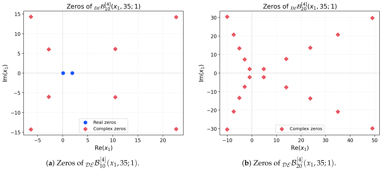
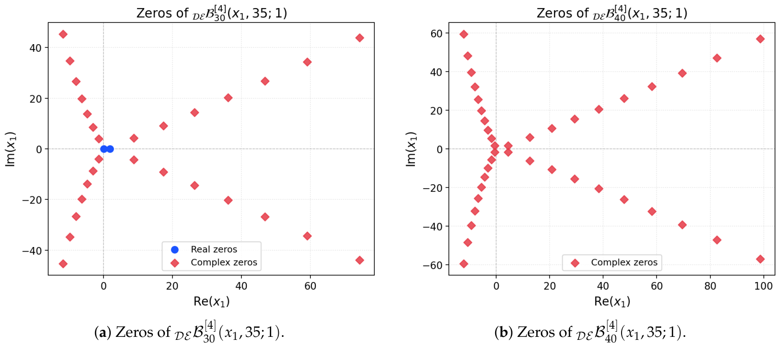
Figure 1 and Figure 2 display our numerical results for the approximate zeros of ${}_{\mathcal{DE}}\mathcal{B}_n^{\left[4\right]}(x_1,35;1)$ for $n=10,20,30$, and 40.

The figures reveal several notable features of the zero distribution of ${}_{\mathcal{DE}}\mathcal{B}_n^{\left[4\right]}(x_1,35;1)$ as the degree n increases. First, the zeros cluster into two distinct groups: a small number of real zeros lying near the interval $[0,1]$, and a much larger collection of complex zeros arranged in conjugate pairs, consistent with Proposition 1(i). Second, the complex zeros are distributed in a pattern exhibiting an approximate four-fold rotational structure in the complex plane, reflecting the order-4 Gould–Hopper kernel ($m=4$). As n grows from 10 to 40, the outermost complex zeros move further from the real axis, with the imaginary parts scaling roughly as $n^{1/4}$, consistent with the degree-m nature of the dominant term in the generating function. Third, the real zeros remain bounded and concentrated near $x_1=\frac{1}{2}$ and the classical Bernoulli zero values, confirming the structural symmetry established analytically in Proposition 1. The increasingly sparse distribution of real zeros relative to complex zeros as n grows suggests that the polynomial family becomes predominantly complex in its zero behaviour for large degrees.

To complement the fixed-parameter plots of Figure 1 and Figure 2, and to illustrate the dependence of the zero structure on the parameters, one may consider a three-dimensional representation showing the zero distribution of ${}_{\mathcal{DE}}\mathcal{B}_n^{\left[4\right]}(x_1,x_2;1)$ for $n=10$ as the parameter $x_2$ varies over the range $x_2\in \{5,15,25,35\}$: each value of $x_2$ contributes one layer of zeros in a three-dimensional scatter plot whose axes are $\mathrm{Re}\left(x_1\right)$, $\mathrm{Im}\left(x_1\right)$, and $x_2$. As $x_2$ increases the complex zeros migrate outward (in modulus) along directions making ${45}^{\circ }$ angles with the real axis, consistent with the dominant term $x_2{\tau }^4$ in the generating function, while the real zeros remain confined to $[0,1]$ for all tested values of $x_2$. The value $\lambda =1$ is chosen because it is the smallest positive integer value, making $log(1+\lambda )=log2$ an explicitly computable constant; the qualitative features described in Proposition 1 hold for all $\lambda >0$, as the proof depends only on the reality of the coefficients and the Bernoulli reflection identity.

Our numerical results for the approximate zeros of ${}_{\mathcal{DE}}\mathcal{B}_n^{\left[4\right]}(x_1,35;1)$ for $1\le n\le 10$ are displayed in

Table 1. Approximate zeros of $x_1$ for each degree n of ${}_{\mathcal{DE}}\mathcal{B}_n^{\left[4\right]}(x_1,35;1)$.

Degree n	${\mathit{x}}_1$ (Zeros)
0	Constant (no zeros)
1	0.7213
2	0.2113, 1.2313
3	0.2113, 0.5, 0.7887
4	−5.2081 − 5.2081 i, −5.2081 + 5.2081 i, 5.7081 − 5.7081 i, 5.7081 + 5.7081 i
5	0.5, −7.8214 − 7.8214 i, −7.8214 + 7.8214 i, 8.3214 − 8.3214 i, 8.3214 + 8.3214 i
6	0.2113, 0.7887, −10.2953 − 10.2953 i, −10.2953 + 10.2953 i, 10.7953 − 10.7953 i, 10.7953 + 10.7953 i
7	0.5, −12.7419 − 12.7419 i, −12.7419 + 12.7419 i, 0.2113, 13.2419 − 13.2419 i, 13.2419 + 13.2419 i, 0.7887
8	−15.1313 − 15.1313 i, −15.1313 + 15.1313 i, −4.2081 − 4.2081 i, −4.2081 + 4.2081 i, 4.7081 − 4.7081 i, 4.7081 + 4.7081 i, 15.6313 − 15.6313 i, 15.6313 + 15.6313 i
9	0.5, −17.4952 − 17.4952 i, −17.4952 + 17.4952 i, −6.6214 − 6.6214 i, −6.6214 + 6.6214 i, 7.1214 − 7.1214 i, 7.1214 + 7.1214 i, 17.9952 − 17.9952 i, 17.9952 + 17.9952 i
10	0.2113, 0.7887, −19.8412 − 19.8412 i, −19.8412 + 19.8412 i, −8.9414 − 8.9414 i, −8.9414 + 8.9414 i, 9.4414 − 9.4414 i, 9.4414 + 9.4414 i, 20.3412 − 20.3412 i, 20.3412 + 20.3412 i

.

Discussion of Table 1. The tabulated values confirm Proposition 1 explicitly for $n=1,\dots ,10$. For odd degrees ($n=1,3,5,7,9$), the value $x_1=0.5$ appears as a zero, consistent with part (iii) of Proposition 1. For even degrees, the real zeros occur in pairs $\{a,1-a\}$ (e.g., $\{0.2113,0.7887\}$ for $n=2,6,8,10$), confirming the reflection symmetry of part (ii). The asymmetric shift of the real parts of the complex zeros away from the imaginary axis is visible throughout the table; this shift is related to the Bernoulli number $B_1=-\frac{1}{2}$, which offsets the zero set from the symmetric configuration that would arise from $g\left(\tau \right)=1$.

Remark 6.

Comparison with the pure degenerate Gould–Hopper case studied in [7] reveals that the presence of the Bernoulli–Appell factor $g\left(\tau \right)=\tau /(e^{\tau }-1)$ breaks the exact conjugate-plus-origin symmetry of the zeros. In particular, the real parts of the complex zeros are no longer symmetric about the imaginary axis; rather, they are shifted by an offset related to the Bernoulli number $B_1=-{\displaystyle \frac{1}{2}}$. The real zeros of the Bernoulli subfamily cluster near the values $x_1\in \{{\displaystyle \frac{1}{2}}-\sqrt{3}/6,{\displaystyle \frac{1}{2}},{\displaystyle \frac{1}{2}}+\sqrt{3}/6\}$, which are the zeros of the Bernoulli polynomials $B_1\left(x_1\right)$, $B_2\left(x_1\right)$, and $B_3\left(x_1\right)$, respectively.

Proposition 1.

Let ${}_{\mathcal{DE}}\mathcal{B}_n^{\left[4\right]}(x_1,35;1)$ be the mixed degenerate Gould–Hopper–Bernoulli-type polynomials of order $m=4$, with $x_1\in \mathbb{R}$. For every integer $n\ge 1$, the following structural properties of the zeros with respect to $x_1$ hold:

(i)

All non-real zeros appear in conjugate pairs, i.e., if $z\in \mathbb{C}\setminus \mathbb{R}$ is a zero, then so is $\overline{z}$.

(ii)

For even n, the complex zeros are arranged in quadruples of the form $\{a\pm bi,(1-a)\pm bi\}$, reflecting the symmetry $x_1\mapsto 1-x_1$ inherited from the Bernoulli polynomial structure.

(iii)

For odd n, the value $x_1={\displaystyle \frac{1}{2}}$ always appears as a zero.

Proof. 

From the explicit series representation established in Theorem 1 with $g\left(\tau \right)=\tau /(e^{\tau }-1)$, $m=4$, $x_2=35$, and $\lambda =1$, we have

$${}_{\mathcal{DE}}\mathcal{B}_n^{\left[4\right]}(x_1,35;1)=n!{\displaystyle \sum _{q=0}^{\lfloor n/4\rfloor }}{\displaystyle \frac{{35}^q}{q!}}·{\displaystyle \frac{{\mathcal{B}}_{n-4q}(x_1;\lambda )}{(n-4q)!}},$$

(67)

where ${\mathcal{B}}_j(x_1;1)$ are the degenerate Bernoulli polynomials at $\lambda =1$.

(i)

Conjugate pairing. The degenerate Bernoulli polynomials ${\mathcal{B}}_j(x_1;1)$ have real coefficients when evaluated at real $\lambda =1$, since all Bernoulli numbers are real and $log\left(2\right)\in \mathbb{R}$. Hence the polynomial ${}_{\mathcal{DE}}\mathcal{B}_n^{\left[4\right]}(x_1,35;1)$ in $x_1$ has exclusively real coefficients. The complex conjugate root theorem then gives: if z is a zero, then

$$0=\overline{{}_{\mathcal{DE}}\mathcal{B}_n^{\left[4\right]}(z,35;1)}={}_{\mathcal{DE}}\mathcal{B}_n^{\left[4\right]}(\overline{z},35;1),$$

(68)

so $\overline{z}$ is also a zero, establishing the conjugate pairing of all non-real zeros.

(ii)

Quadruple symmetry for even $\mathit{n}$. The Bernoulli polynomial satisfies the reflexion identity ${\mathcal{B}}_j(1-x_1)={(-1)}^j{\mathcal{B}}_j\left(x_1\right)$ for all $j\ge 0$. Substituting $x_1\mapsto 1-x_1$ into the explicit sum and using this identity:

$${}_{\mathcal{DE}}\mathcal{B}_n^{\left[4\right]}(1-x_1,35;1)=n!{\displaystyle \sum _{q=0}^{\lfloor n/4\rfloor }}{\displaystyle \frac{{35}^q}{q!}}·{\displaystyle \frac{{(-1)}^{n-4q}{\mathcal{B}}_{n-4q}(x_1;1)}{(n-4q)!}}.$$

(69)

When n is even, each exponent $n-4q$ is even, so ${(-1)}^{n-4q}=1$, and thus

$${}_{\mathcal{DE}}\mathcal{B}_n^{\left[4\right]}(1-x_1,35;1)={}_{\mathcal{DE}}\mathcal{B}_n^{\left[4\right]}(x_1,35;1).$$

(70)

Therefore, if z is a zero, so is $1-z$. Combined with the conjugate symmetry from part (i), each non-real non-half-integer zero $z=a+bi$ with $a\ne {\displaystyle \frac{1}{2}}$ belongs to the quadruple $\{a\pm bi,(1-a)\pm bi\}$.

(iii)

Zero at ${\mathit{x}}_{\mathbf{1}}={\displaystyle \frac{\mathbf{1}}{\mathbf{2}}}$ for odd $\mathit{n}$. When n is odd, the same substitution gives ${(-1)}^{n-4q}=-1$ for each term (since $n-4q$ is odd when n is odd), yielding

$${}_{\mathcal{DE}}\mathcal{B}_n^{\left[4\right]}(1-x_1,35;1)=-{}_{\mathcal{DE}}\mathcal{B}_n^{\left[4\right]}(x_1,35;1).$$

(71)

Setting $x_1={\displaystyle \frac{1}{2}}$ in this identity gives ${}_{\mathcal{DE}}\mathcal{B}_n^{\left[4\right]}({\displaystyle \frac{1}{2}},35;1)=-{}_{\mathcal{DE}}\mathcal{B}_n^{\left[4\right]}({\displaystyle \frac{1}{2}},35;1)$, and hence ${}_{\mathcal{DE}}\mathcal{B}_n^{\left[4\right]}({\displaystyle \frac{1}{2}},35;1)=0$. Therefore $x_1={\displaystyle \frac{1}{2}}$ is always a zero for odd n.

□

6. Conclusions

This article has introduced the Mixed Degenerate Gould–Hopper–Appell-Type Polynomials ($MDGHA$-$TPs$) by combining, within a single two-variable generating function, the Appell factor $g\left(\tau \right)$, the degenerate exponential kernel ${(1+\lambda \tau )}^{x_1/\lambda }$, and the Gould–Hopper kernel $exp\left(x_2{\tau }^m\right)$. From this definition we have derived, in sequence: explicit series representations in terms of the underlying degenerate Appell polynomials; reduction formulas recovering the degenerate Appell family at $x_2=0$ and the degenerate exponential polynomials at $x_1=0$; multiplicative and derivative operators establishing quasi-monomiality, together with the associated partial differential equation; summation identities involving Stirling numbers of the first kind, bivariate addition formulas, and a convolution identity; and a determinantal representation of the family [30].

The lower Hessenberg determinantal form of Theorem 9 is particularly significant: it provides an explicit, recursion-free representation of every member of the family, making the recursive dependence among family members both transparent and computationally efficient. The differential equation of Theorem 5 characterises the $MDGHA$-$TPs$ as eigenfunctions of the operator ${\widehat{\mathcal{M}}}_{\mathcal{A}}{\widehat{\mathcal{D}}}_{\mathcal{A}}$ with eigenvalue n; in the classical limit $\lambda \to 0$ it reduces to the known differential equation for Gould–Hopper–Appell polynomials, while for $\lambda \ne 0$ it describes a genuinely new degenerate spectral problem.

A particular focus of the computational part is the zero distribution of the Bernoulli subfamily ${}_{\mathcal{DE}}\mathcal{B}_n^{\left[4\right]}(x_1,35;1)$. Compared to the pure degenerate Gould–Hopper case, where the zeros are symmetric about the imaginary axis, the Bernoulli factor shifts this symmetry by $\frac{1}{2}$: the zero set satisfies the reflexion $x_1\leftrightarrow 1-x_1$, which is the hallmark of the Bernoulli family. The proof that $x_1=\frac{1}{2}$ is a zero for every odd n makes this structural coupling precise and shows that the Appell factor influences the zero distribution in a quantitatively controlled way.

The following open problems are identified for future research.

1.

Orthogonality. A natural problem is to determine whether the $MDGHA$-$TPs$ satisfy orthogonality conditions with respect to suitable weight functions, perhaps through a degenerate or generalised inner-product formalism; a positive answer would contribute substantially to their spectral theory.

2.

Asymptotic zero distribution. It would be worthwhile to study the limiting zeros of the moduli of these polynomials and interlacing phenomena; this would allow for connections to potential theory and logarithmic capacity to be made.

3.

q-deformations. The definition of the sequence of $MDGHA$-$TPs$ naturally lends itself to q-deformations or fractional powers of the Appell factor and degenerate exponential, thus yielding hybrid families with applications to quantum discrete calculus.

4.

Umbral calculus. An umbral calculus approach would shed light on the significance of the degeneracy parameter $\lambda$, while uncovering relations between the different polynomials used.

5.

Integral representations. Adapting the methods of Cesarano [26,27] for multi-dimensional Hermite and Chebyshev polynomials to the degenerate Gould–Hopper–Appell setting is a natural direction for future work.

6.

Applications. Due to the connection to higher-order heat equations and diffusion processes, the $MDGHA$-$TPs$ have the potential to serve as efficient tools for solving boundary value problems in non-homogeneous media, for signal processing, and for perturbation expansions in quantum mechanics.

From an applied perspective, the $MDGHA$-$TPs$ are naturally suited to several computational and physical contexts. In quantum mechanics, Gould–Hopper polynomials of order $m=4$ arise in the perturbative treatment of anharmonic oscillators with quartic potentials; the presence of the degenerate exponential factor ${(1+\lambda \tau )}^{x_1/\lambda }$ provides a one-parameter regularisation that controls the classical limit and may be relevant for lattice discretisations of the Schrödinger equation. In heat conduction theory, the Appell–Gould–Hopper structure encodes solutions to higher-order diffusion equations of the form ${\partial }_{t}u=c{\partial }_x^{m}u$ with inhomogeneous initial data encoded by $g\left(\tau \right)$; the degenerate variant studied here corresponds to a discrete-time or finite-difference version of this equation. In signal processing, the mixed polynomial family provides a flexible basis for approximating functions that exhibit both Gaussian and higher-order algebraic decay, with the deformation parameter $\lambda$ offering an additional degree of freedom for fitting.

References

1. Andrews, L.C. Special Functions for Engineers and Mathematicians; Macmillan: New York, NY, USA, 1985. [Google Scholar]
2. Erdélyi, A.; Magnus, W.; Oberhettinger, F.; Tricomi, F.G. Higher Transcendental Functions; Krieger: New York, NY, USA, 1981; Volume 1. [Google Scholar]
3. Andrews, G.E.; Askey, R.; Roy, R. Special Functions; Cambridge University Press: Cambridge, UK, 1999. [Google Scholar]
4. Arfken, G. Mathematical Methods for Physicists, 3rd ed.; Academic Press: San Diego, CA, USA, 1985. [Google Scholar]
5. Dattoli, G. Generalized polynomials: Operational identities and their applications. J. Comput. Appl. Math. 2000, 118, 111–123. [Google Scholar] [CrossRef]
6. Khan, S.; Yasmin, G.; Khan, R.; Hassan, N.A.M. Hermite-based Appell polynomials: Properties and applications. J. Math. Anal. Appl. 2009, 351, 756–764. [Google Scholar] [CrossRef]
7. Wani, S.A.; Warke, A.; Dar, J.G. Degenerate 2D bivariate Appell polynomials: Properties and applications. Appl. Math. Sci. Eng. 2023, 31, 2194645. [Google Scholar] [CrossRef]
8. Wani, S.A. Two-iterated degenerate Appell polynomials: Properties and applications. Arab J. Basic Appl. Sci. 2024, 31, 83–92. [Google Scholar] [CrossRef]
9. Wani, S.A.; Khan, S. Certain properties and applications of the 2D Sheffer and related polynomials. Bol. Soc. Mat. Mex. 2020, 26, 947–971. [Google Scholar] [CrossRef]
10. Ryoo, C.S.; Khan, W.A. On two bivariate kinds of poly-Bernoulli and poly-Genocchi polynomials. Mathematics 2020, 8, 417. [Google Scholar] [CrossRef]
11. Wani, S.A.; Riyasat, M.; William, R.; Khan, W.A. Multivariate q-Hermite-based Appell polynomials: Structural properties and applications. Afr. Mat. 2025, 36, 97. [Google Scholar] [CrossRef]
12. Cesarano, C.; Quintana, Y.; Ramírez, W. Degenerate versions of hypergeometric Bernoulli-Euler polynomials. Lobachevskii J. Math. 2024, 45, 3509–3521. [Google Scholar] [CrossRef]
13. Hermite, C. Sur un nouveau développement en série de fonctions. C. R. Acad. Sci. Paris 1864, 58, 93–100, 266–273. [Google Scholar]
14. Appell, P.; Kampé de Fériet, J. Fonctions Hypergéométriques et Hypersphériques: Polynômes d’Hermite; Gauthier-Villars: Paris, France, 1926. [Google Scholar]
15. Gould, H.W.; Hopper, A.T. Operational formulas connected with two generalizations of Hermite polynomials. Duke Math. J. 1962, 29, 51–63. [Google Scholar] [CrossRef]
16. Appell, P. Sur une classe de polynômes. Ann. Sci. École Norm. Sup. 1880, 9, 119–144. [Google Scholar] [CrossRef]
17. Cesarano, C.; Ramírez, W.; Khan, S. A new class of degenerate Apostol-type Hermite polynomials and applications. Dolomites Res. Notes Approx. 2022, 15, 1–10. [Google Scholar]
18. Ramírez, W.; Cesarano, C.; Díaz, S. New results for degenerated generalized Apostol-Bernoulli, Apostol-Euler and Apostol-Genocchi polynomials. WSEAS Trans. Math. 2022, 21, 604–608. [Google Scholar] [CrossRef]
19. Carlitz, L. Degenerate Stirling, Bernoulli and Eulerian numbers. Util. Math. 1979, 15, 51–88. [Google Scholar]
20. Cenkci, M.; Howard, F.T. Notes on degenerate numbers. Discret. Math. 2007, 307, 2359–2375. [Google Scholar] [CrossRef]
21. Young, P.T. Degenerate Bernoulli polynomials, generalized factorial sums, and their applications. J. Number Theory 2008, 128, 738–758. [Google Scholar] [CrossRef]
22. Wani, S.A.; Nisar, K.S. Quasi-monomiality and convergence theorem for Boas-Buck-Sheffer polynomials. Mathematics 2020, 5, 4432–4453. [Google Scholar] [CrossRef]
23. Dattoli, G. Hermite-Bessel and Laguerre-Bessel functions: A by-product of the monomiality principle. Adv. Spec. Funct. Appl. 1999, 1, 147–164. [Google Scholar]
24. Dattoli, G.; Lorenzutta, S.; Cesarano, C. Generalized polynomials and new families of generating functions. Ann. Univ. Ferrara Sez. VII 2001, 47, 57–61. [Google Scholar] [CrossRef]
25. Steffensen, J.F. The poweriod, an extension of the mathematical notion of power. Acta Math. 1941, 73, 333–366. [Google Scholar] [CrossRef]
26. Cesarano, C. Integral representations and new generating functions of Chebyshev polynomials. Hacet. J. Math. Stat. 2015, 44, 535–546. [Google Scholar] [CrossRef]
27. Cesarano, C. Multi-dimensional Chebyshev polynomials: A non-conventional approach. Commun. Appl. Ind. Math. 2019, 10, 1–19. [Google Scholar] [CrossRef]
28. Gould, H.W. Stirling number representation problems. Proc. Amer. Math. Soc. 1960, 11, 447–451. [Google Scholar] [CrossRef]
29. Abramowitz, M.; Stegun, I.A. Stirling numbers of the second kind. In Handbook of Mathematical Functions with Formulas, Graphs, and Mathematical Tables, 9th ed.; Dover: New York, NY, USA, 1972; pp. 824–825. [Google Scholar]
30. Costabile, F.A.; Gualtieri, M.I.; Napoli, A. Recurrence relations and determinant forms for general polynomial sequences: Application to Genocchi polynomials. Integral Transform. Spec. Funct. 2025, 36, 1–18. [Google Scholar] [CrossRef]
Figure 1. Zero distribution of B n [ 4 ] DE ( x 1 , 35 ; 1 ) for n = 10 , 20 .
Symmetry 18 00901 g001
Figure 2. Zero distribution of B n [ 4 ] DE ( x 1 , 35 ; 1 ) for n = 30 , 40 .
Symmetry 18 00901 g002