


Abstract
The chiral quark soliton model (CQSM) is an effective quark model of baryons maximally taking account of the most important feature of low-energy QCD, i.e., the spontaneous chiral symmetry breaking of the QCD vacuum and the associated appearance of Nambu–Goldstone pions. It shares many common features with the famous Skyrme model in that the baryons are viewed as rotating hedgehog objects in both models. Despite many similarities, it turned out that the CQSM can give more realistic predictions on most baryon observables. Above all, a decisive advantage of the CQSM over the Skyrme-like models is that it can handle non-local quark–quark correlations in baryons, which is absolutely impossible within the framework of effective meson theories. This feature is decisively important for making theoretical predictions on the quark distribution functions inside the nucleon, which are defined as nucleon matrix elements of bilinear quark operators with light-cone separation. In the present paper, we try to elucidate why and how the CQSM can give successful predictions for a variety of types of nucleon quark distribution functions, especially for the flavor asymmetry of the unpolarized and longitudinally polarized sea-quark (anti-quark) distribution functions in the nucleon.
1. Introduction
It is widely believed that the most important properties of the quantum chromodynamics (QCD) are the color confinement and the asymptotic freedom. However, from the perspective of the low-energy phenomenology of hadron physics, there is an even more important property of QCD. It is the spontaneous chiral symmetry breaking of the QCD vacuum and the associated appearance of the Nambu–Goldstone bosons. The chiral quark soliton model (CQSM) is an effective theory of QCD, which efficiently incorporates this important dynamical symmetry of QCD into the physics of baryon structures [1]. (Earlier reviews of the model can, for example, be found in [2,3]; see also [4].) In short, the theoretical framework of the CQSM is a relativistic mean field theory for quark fields. The quarks in the nucleon or any baryons are supposed to move in a mean field of hedgehog shape with nontrivial topology. (Remember that the classical pion field configuration of the hedgehog shape is the core of the Skyrme model as an effective meson theory of baryons [5].) By taking account of nonperturbative deformation (or vacuum polarization) of the negative-energy Dirac-sea quark orbitals under the influence of the hedgehog mean field, the CQSM automatically and effectively incorporates pionic quark–antiquark excitation modes inside the baryons. In fact, the model turned out to reproduce a lot of baryon observables fairly well with almost no free parameters.
Probably, the most successful application of the CQSM lies in excellent reproduction of the parton distribution functions (PDFs) in the nucleon [6,7,8,9,10,11,12,13]. Among others, predicted flavor asymmetries of the sea-quark (or anti-quark) distributions for both the unpolarized PDFs and the longitudinally polarized PDFs are surprisingly consistent with the observational data accumulated to date, which in turn proves the importance of the chiral symmetry embedded in the physics of nucleon parton distribution functions [12,13]. In the present paper, we shall review how and why the CQSM can explain many characteristic features of the parton distribution functions of the nucleon, mainly focusing on our own contributions.
The paper is organized as follows. First, in Section 2, we briefly explain what the CQSM is like. Also shown are several noteworthy features of the theoretical predictions of the CQSM for nucleon observables. In Section 3, we explain how we can calculate the quark and anti-quark distribution functions in the nucleon. The distribution functions given at the low-energy model scale, which is thought to be around , are then evolved to high energy scale, where the experimental data obtained from the deep-inelastic scattering measurements exist. Next, in Section 4, the flavor SU(3) extension of the CQSM is explained. The greatest advantage of this extension is that it enables us to make nontrivial predictions about the asymmetry of the strange and anti-strange quark distributions in the nucleon. In Section 5, short remarks are made on our current understanding of the gauge-invariant decomposition problem of the nucleon spin. Next, in Section 6, we discuss the generalized form factors and Ji’s angular momentum sum rule of the nucleon [14,15]. In Section 7, based on Ji’s sum rule explained in the previous section, we shall carry out a semi-empirical analysis of the nucleon spin contents, especially by paying attention to their scale dependencies. Finally, in Section 8, we make some comments on the future prospects, based on the discussion in the present paper.
2. Brief Introduction to Chiral Quark Soliton Model
The chiral quark soliton model (CQSM) is a low-energy effective model of baryons first proposed by Diakonov, Petrov, and Pobilitsa based on the instanton-liquid picture of the QCD vacuum [1]. The basic Lagrangian of the CQSM is very simple and given as
with . Here, stands for the isospin-triplet pion fields. (In the flavor SU(3) version of the CQSM, the pion fields here should be replaced by the octet meson fields.) The Lagrangian above describes the effective quark fields nonlinearly coupled to the Nambu–Goldsto pion fields . Here is one important point to note. The pions in this model Lagrangian are not independent fields of quarks, as indicated by the fact that there is no kinetic term of the pion fields in the above Lagrangian. The kinetic terms of the pions are thought to be generated as a quantum effect. In fact, if one constructs an effective meson action from the flavor SU(3) version of the above effective quark Lagrangian by integrating out the quark fields with the use of the derivative expansion method, it is known to reproduce the famous Skyrmion action with the Wess–Zumino term, but together with soliton destabilizing 4th derivative terms [5]. Actually, we do not use such an approximate bosonization formalism.
The central idea of the CQSM is a soliton construction without recourse to approximate a bosonization procedure. We start with a classical pion field configuration with a hedgehog shape as follows, which plays the role of a mean field for quarks:
Here, the profile function is supposed to satisfy the following boundary condition,
with being the so-called winding number of the effective pion field configuration. Under the presence of this unique shape of mean field, the quark field obeys the following Dirac equation,
with
Here, M is supposed to stand for the dynamical quark mass (or the constituent quark mass) generated by the spontaneous chiral symmetry breaking of the QCD vacuum. A characteristic feature of the above Dirac equation is that one deep bound state emerges from the positive-energy Dirac continuum (see Figure 1). Hereafter, we call this quark orbit the valence quark level. Then, a baryon-number-one object with respect to the physical vacuum is obtained by putting -quarks into this valence orbital as well as all the negative-energy Dirac-sea orbitals.
Figure 1.
Characteristic behavior of the single-quark energy levels under the hedgehog mean field.
Accordingly, the total energy of this baryon-number-one object is given as a sum of the energy of valence quarks and the energy of deformed (vacuum-polarized) Dirac-sea quarks as
Here, represents the single-particle energy of the valence quark orbital, while the vacuum polarization contribution corresponds to the Casimir energy resulting from the polarization (deformation) of the Dirac-sea quark orbitals. The latter is given as
That is, the Casimir energy is given as a sum of all the energies of quarks in the negative-energy Dirac-sea orbitals. The 2nd term here represents the subtraction of the Dirac-sea energy of the physical vacuum, which is obtained by letting . The most probable pion field configuration is then determined from the stationary requirement for the total energy functional ,
This requirement combined with the above Dirac equation is reduced to a self-consistent Hartree problem which can be solved by the numerical method of Kahana, Ripka, and Soni [16,17]. (See [18] for more details about the actual calculation method.) After self-consistency is fulfilled, the hedgehog pion field, which was originally introduced as an external mean field for quarks, becomes an implicit functional of the quark fields.
Actually, the vacuum polarization energy given by Equation (7) contains ultraviolet divergence (logarithmic divergence). Often, this ultraviolet divergence is removed with the use of the Pauli–Villars regularization, which means the following replacement of the effective action [6,7]
where is a Pauli–Villars cutoff mass. For a given dynamical quark mass M, the Pauli–Villars mass is fixed from the following condition
with being the pion weak-decay constant. This condition follows from the requirement that the above regularized action reproduces the correct pion kinetic term after bosonization. For some special quantities, like the vacuum quark condensate as well as the nucleon scalar charge, however, the above single-term Pauli–Villars subtraction is not enough, because those quantities contain quadratic divergence. For handling those special quantities, we must use more sophisticated double-term Pauli–Villars subtraction, as discussed in [19], which requires the following replacement of the effective action:
Four subtraction parameters are determined so as to remove quadratic and logarithmic divergence of the effective action and to reproduce the empirical value of vacuum condensate and correct pion kinetic energy term in the effective pion action [19]. Once these parameters are fixed, the model does not contain any other free parameters.
The quark hedgehog state constructed on the basis of the hedgehog mean field breaking the rotational symmetry in the coordinate space as well as in the isospin space, so that it is not a good spin–isospin eigen-state. This comes from the degeneracy of the static energy under the rotation in the coordinate and isospin spaces. (Remember the analogous situation that happens for the baryon-number-one object in the Skyrme model [20,21].) This naturally generates a spontaneous (zero-mode) rotation of the hedgehog mean field, which can be parametrized as
where is a time-dependent matrix describing the rotation of the hedgehog mean field in the coordinate and isospin spaces. Now the spin–isospin projection of the rotating hedgehog is carried out by using the cranking method familiar in nuclear physics [22], which consists of the following procedures:
- •
- Cranked iso-rotation of hedgehog mean field induces Coriolis coupling acting on the quarks in the rotating frame given by
- •
- Evaluate changes of the intrinsic quark wave function and the associate changes of observables by treating the above Coriolis coupling as an external perturbation.
- •
- Canonically quantize the iso-rotational motion.
Although the detail is skipped here, the final formula for evaluating baryon observables is given in the following form, i.e., in the form that the effective operator as a function of the collective coordinates A is sandwiched by the wave functions describing the collective rotational motion of hedgehog mean field as [1,18]
Here, is the wave function describing the collective rotational motion of the baryon states and is given as
where is the familiar Wigner rotation matrix. The effective operator consists of the zeroth and the first-order terms in the collective angular velocity as
The lowest order term just corresponds to the answer in the mean field theory, and it is given as a diagonal sum over the occupied states consisting of the valence quark orbital with the energy and all the negative-energy Dirac-sea orbitals with as
with
In the above equation, stands for the sum over the occupied quark orbitals n. On the other hand, the term or the correction term is given as a double sum over the occupied orbitals n and the non-occupied orbitals m as follows:
which describes virtual transitions from the occupied states to the non-occupied states by the action of the external field and the Coriolis force and vice versa.
Here we summarize several noteworthy features of the predictions of the CQSM for nucleon observables.
- (1)
- Good reproduction of the neutron charge distribution as a clear evidence of efficiently incorporating the pion cloud effect.
- (2)
- Resolution of the famous underestimation problem of the isovector axial-vector coupling constant of the nucleon in the Skyrme model.
- (3)
- Reproduce a large sigma term consistent with the empirical information as well as highly nontrivial behavior of the scalar quark density of the nucleon in coordinate space and momentum space.
- (4)
- Good reproduction of the small quark spin fraction of the nucleon consistent with the high-energy deep-inelastic-scattering data by the EMC group.
- Following are supplementary explanations concerning the above-mentioned remarkable features of the model predictions.
- (1)
- We first explain the reason why good reproduction of the neutron charge distribution is a noteworthy matter [23]. Shown in Figure 2 is the prediction of the CQSM for the neutron charge distribution. The dashed curve represents the contribution of the valence quarks to the neutron charge density. Note that the contribution from the valence quarks is positive in most spatial regions and its magnitude rapidly decreases as the distance r from the neutron center becomes large. The dash-dotted curve in the same figure shows the contribution from the negative-energy Dirac-sea quarks. As one sees, this contribution is negative in all the region but it has a long-range tail as r becomes large as compared with the contribution of the valence quarks. Probably, the above feature can be understood based on the well-known meson theory of Yukawa. In this theory, the physical neutron is thought to virtually dissociate into the superposition state of the proton and the as . Since the is much lighter than the proton (and the neutron), it virtually travels far away from the center of the neutron. This results in a centrally concentrated positive charge distribution by the virtual proton and a negative charge distribution by the virtual that dominates in the outer region. (The charge conservation naturally ensures that the net charge of the neutron is zero.) We think that the contribution of the three valence quarks in the CQSM simulates the positive charge distribution due to the virtual proton, while the contribution from the Dirac-sea quark simulates the negative charge distribution due to the cloud of . Undoubtedly, the neutron charge distribution is thought to provide the simplest clear evidence showing the importance of the chiral symmetry of QCD, which is efficiently taken into account into the framework of the CQSM.Figure 2. The CQSM prediction for the neutron charge density multiplied by . The dashed and dash-dotted curves respectively stand for the contribution of the valence quarks and the negative-energy Dirac-sea quarks, while the solid curve represents their sum.
- (2)
- Although it was not necessarily taken seriously, there was a sizable underestimation problem of the isovector axial-vector coupling constant of the nucleon in the Skyrme model [20,21]. As compared with the empirically known value , the prediction of the Skyrme model is known to be around . One might think that this is a minor problem concerning a tiny flaw of a model. However, this problem was not solved within the Skyrme model, and it turned out to persist in any soliton models based on the hedgehog configuration within effective Lagrangians of mesons [24,25,26]. As already pointed out, there are many common features between the Skyrme model and the CQSM. Somewhat unexpectedly, however, we noticed that, within the framework of the CQSM, there is an important 1st-order rotational correction in the collective angular velocity (it is also thought of as a novel correction), which is completely missing in the framework of the Skyrme model [27,28]. In fact, it turned out that these two models give the following prediction on :It was argued that there is a deep reason for this critical difference between the prediction of the CQSM as an effective fermion theory and that of the Skyrme model as an effective meson theory [29,30]. From more fundamental standpoint based on an effective theory at the quark level, we can say that the ultimate origin of the problem in the Skyrme model comes from the non-commutativity of the bosonization procedure and the collective quantization procedure. (For more detail, we refer to the literature above [29,30].) In short, an important piece of information of the original fermion theory is lost in the process of the bosonization procedure. Aside from this fundamental difference, we emphasize that the CQSM generally gives more realistic physical predictions on most baryon observables than the Skyrme model. Besides, as we shall discuss in the following, the most important advantage of the CQSM as compared with the Skyrme model is that the former can handle the non-local quark–quark correlation inside the nucleon, which is necessary to evaluate the quark distribution functions of the nucleon, while there is no way to handle such non-local quark–quark correlation within the theoretical framework of effective meson theories of baryons, including the Skyrme model.
- (3)
- Probably, a highly unique feature of the CQSM is that it simultaneously reproduces nontrivial local chiral structure of the nucleon and the QCD vacuum structure with nonzero quark condensate [19,31]. It can be seen from Figure 3, which shows the model prediction of the nucleon scalar charge density in the QCD vacuum. The dashed curve and the dash-dotted curve here respectively denote the contribution of the valence quarks and that of the Dirac-sea quarks to the nucleon scalar quark density, while their sum is shown by the solid curves. One can see that the contribution of the valence quarks smoothly attenuates to zero as the distance from the nucleon center becomes large, as is the case with the predictions of almost all models of the nucleon. Remarkably, however, the contribution of the negative-energy Dirac-sea quarks does not attenuate to zero, but it rather approaches a negative value, which is nothing but the value of the QCD vacuum quark condensate. This means that the CQSM can explain the vacuum quark condensate and the nontrivial local structure of the nucleon scalar charge density simultaneously. One may naturally anticipate that this extraordinary structure of the nucleon scalar charge density would show itself in some observables. It was shown to appear as a delta-function type singularity in the twist-3 chiral-odd quark distribution function of the nucleon [32,33,34]. Since this topic was intensively discussed in a recent review paper [35], we do not discuss it further in the present paper.Figure 3. The CQSM prediction of the nucleon scalar charge density. The dashed and dash-dotted curves respectively stand for the contributions from the valence quarks and the Dirac-sea quarks, while the solid curve represents the total contribution.
- (4)
- Another prominent feature of the CQSM is that it predicts fairly small quark spin fraction of the nucleon as [11]at the energy scale of the model, which is thought to be around . Since the CQSM is an effective theory of quarks, which does not explicitly contain the gluon degrees of freedom, it satisfies the following sum rule of the nucleon spin [18]where represents the contribution of the intrinsic quark spin, while represents the contribution of the quark orbital angular momentum to the net nucleon spin. The smallness of the quark spin fraction therefore implies the largeness of the contribution of the orbital angular momentum of quarks. Undoubtedly, the largeness of the orbital angular momentum contribution is inseparably connected with the basic dynamical assumption of the CQSM, i.e., its nucleon picture as a rotating hedgehog object.
So far, we have demonstrated that the CQSM model is able to explain important characteristics of several nucleon observables, in which the dynamical chiral symmetry of QCD plays a critically important role. Still, most low-energy baryon observables are insensitive to the differences between low-energy effective models like the MIT bag model and the non-relativistic quark model, etc. In the following sections, we shall show that the potential ability of the CQSM manifests most clearly in its predictions about the internal partonic structure of the nucleon.
3. CQSM and Nucleon Parton Distribution Functions
For obtaining the distribution functions of quarks, we need to evaluate nucleon matrix elements of quark bilinear operators with the light-cone separation given as
with the definition of the standard light-cone coordinates . Here, represents the nucleon state with momentum P. (It is the Lorentz-boost invariance of the quark distribution function along the -axis, i.e., the direction of the momentum of the parent nucleon, that allows us to evaluate the above matrix elements in the nucleon rest frame.) We set and for the isoscalar unpolarized distribution function and the isovector unpolarized distribution function . On the other hand, we take and for the isoscalar longitudinally polarized distribution function and the isovector longitudinally polarized distribution function . On account of the charge conjugation properties of relevant operators, we can formally extend the defining region of quark distribution functions to the interval as
(For readers who are not familiar with the above relations, we shall explain its theoretical basis in Appendix A.)
In the above four equations, the variable x is supposed to lie in the physical range . These relations mean that the quark distributions in the negative x region can actually be interpreted as the corresponding anti-quark distributions after taking care of differences in signs. We also point out that the following novel (∼) dependencies follow from the theoretical structure of the model, i.e., the mean field of hedgehog shape and the subsequent perturbative treatment of the collective rotational motion [6,7]:
Here, and respectively stand for the unpolarized distribution functions of the u-quark and the d-quark, while and represent the longitudinally polarized distribution functions of the u-quark and the d-quark.
Just for reference, we write down the theoretical expressions for the above four basic distribution functions of the nucleon. They are given as [6,7,8,9,10,11]
with the definition . Since the expression of the contribution to is fairly complicated, it is omitted here.
Shown in Figure 4 are the CQSM predictions for the basic twist-2 quark distribution function of the nucleon. The four panels (a), (b), (c), and (d) respectively stand for the isoscalar unpolarized distribution , the isovector unpolarized distribution , the isoscalar longitudinally polarized distribution , and the isovector longitudinally polarized distributions . These figures already show highly nontrivial structure of the quark distribution functions predicted by the CQSM in the small x region and in the negative x region. Remember that the quark distributions in the negative x region can be interpreted as anti-quark distributions aside from signs. In particular, these nontrivial predictions for the anti-quark distributions are inseparably connected with the basic feature of the CQSM, which enables us to take account of nonperturbative vacuum-polarization of the negative-energy Dirac-sea quarks in the hedgehog mean field.
Figure 4.
The CQSM prediction for the twist-2 quark distribution functions of the nucleon. (a) Isoscalar unpolarized distribution, (b) isovector unpolarized distribution, (c) isoscalar longitudinally polarized distribution, (d) isovector longitudinally polarized distribution. In these figures, the dashed curve, the dash-dotted, and the solid curves respectively represent the contributions from the valence quarks, the Dirac-sea quarks, and the sum of them.
One can see that, in any of these four distribution functions, the Dirac-sea quarks give important and characteristic contributions. Worthy of special mention at this stage is the isoscalar unpolarized distribution . The contribution of the valence quarks to this distribution has a peak around the value of , but it has a tail with a positive sign extending to the negative region of x. We emphasize that basically the same behavior is also predicted by most three-quark models of the nucleon, like the non-relativistic quark model and also that of the MIT bag model. However, these predictions are unacceptable, if we remember the relation with , which means that in the negative x region is identified with the anti-quark distribution for a physical value of , but with an extra minus sign. Accordingly, once we discard the contribution of the Dirac-sea contribution, the positivity of the valence quark contribution in the negative x region breaks the positivity of the anti-quark distribution for the physical value of x. Amazingly, however, if the Dirac-sea contribution is properly taken into account, the net contribution to in the negative x region is definitely negative, which means that the prediction of the CQSM legitimately satisfies the required positivity requirement for the anti-quark distribution (See Figure 5). This feature is one of the great advantages of the CQSM as a field-theoretical model of the nucleon [6].
Figure 5.
On the noteworthy feature of the CQSM prediction for the distribution , which ensures the positivity of the anti-quark distribution functions with a physical value of x.
Unfortunately, the above interesting predictions of the CQSM cannot be immediately compared with the empirically known distribution functions, which are obtained from the analyses of the high energy deep-inelastic-scattering (DIS) data. The reason is that the quark distribution functions are in general renormalization-scale (or energy-scale)-dependent quantities. In fact, the above predictions of the CQSM for the quark distribution functions of the nucleon are interpreted to correspond to the distribution functions at the energy scale around 600 MeV, or , which is to be identified with the energy scale of the effective model. On the other hand, the quark distribution function extracted from the high-energy deep-inelastic-scattering (DIS) experiments are known to correspond to a high energy scale, say at least above . A frequently used strategy is to connect the model predictions given at the low energy scale and the empirically known distribution functions through the Dokshitzer–Gribov–Lipatov–Altarelli–Parisi (DGLAP) evolution equation, which is basically the perturbative renormalization group (RG) equation. An immediate question here is whether it is legitimate to use such a perturbative RG equation at a low energy scale, especially because the QCD running coupling constant is known to show diverging behavior as within the perturbative treatment of QCD.
Shown in Figure 6 is the QCD running constant at the next-to-leading order (NLO) as a function of . One sees that, at the low energy scale around 600 MeV, the perturbative QCD treatment looks barely applicable. (This should be contrasted with the fact that the initial scale of evolution in most low-energy models of QCD like the MIT bag model or the cloudy bag model is around . The running coupling constant at this energy is seen to be close to unity, which cannot be thought of as a small parameter in perturbation theory.) This would enable us to use the DGLAP equation at NLO to relate the predictions of the CQSM for PDFs with the empirical PDFs corresponding to high energy scales.
Figure 6.
The QCD running coupling constant at the next-to-leading order (NLO) as a function of the renormalization scale .
The CQSM predictions for the basic twist-2 PDFs are evolved to high energy scales by using the fortran programs provided in the references [36,37]. A difficult problem here is that, to solve the evolution equations in the flavor singlet channel, we also need the gluon distribution functions at the starting low energy scale, but a nonperturbative evaluation of the gluon distribution is impossible in any low-energy effective model of baryons, including the CQSM. The frequently used strategy is to assume that the gluon distributions at the low energy scale are negligibly small and to set zero. Based on our experience so far, there is a noteworthy difference between the two types of gluon distributions, i.e., the unpolarized gluon distribution and the longitudinally polarized gluon distribution. First, consider the net gluon spin as the 1st moment or the integral of the longitudinally polarized gluon distribution . An interesting trial analysis would be as follows. Suppose that, starting from the empirical information for given at the high energy scales, for example, the information given by DSSV fit at , we solved the evolution equation at the next-to-leading order to estimate the value of at the lower energy scales. (This means somewhat unconventional downward evolution or disevolution of the parton distribution functions.) Then, we observe that, as decreases, the magnitude of gradually reduces, and it eventually becomes zero approximately around the energy scale . This indicates that, just around the model energy scale of the CQSM, the contribution of the gluon to the net nucleon spin is fairly small, which in turn indicates the smallness of the longitudinally polarized gluon distribution. In fact, that this consideration is not off the mark can also be confirmed by the following observation. In our treatment, the predictions of the flavor singlet piece of the longitudinally polarized quark distributions at a high energy scale are obtained by solving the coupled evolution equations for the quarks and gluon. The initial quark distributions at the low energy scale are taken from the theoretical predictions of the CQSM, while the longitudinally polarized gluon distribution at this low energy scale is assumed to be zero. Curiously, we found that such a strategy works fairly well, at least to reproduce the empirically known behavior of the longitudinally polarized quark distributions at the high energy scales.
The situation is a little different for the unpolarized quark and gluon distribution functions. Starting from the empirical information for the quark and gluon momentum fractions, and , suppose that we carry out a similar downward evolution to estimate the magnitudes of the quark and gluon momentum fractions at the lower energy scales. Then, we found that, even at the low energy scale around , the gluon still maintains non-negligible momentum fraction. This naturally indicates that the unpolarized gluon distribution is likely to have a sizable magnitude even at such low energy scales. This would also make the CQSM prediction for the flavor singlet combination of the unpolarized quark distributions less reliable as compared with the corresponding predictions for the flavor–nonsinglet combination of the unpolarized quark distributions as well as with the longitudinally polarized quark distributions. As is widely believed, nonperturbative evaluation of the gluon distribution is feasible only within the framework of lattice QCD. However, it may take some time to be able to make really trustworthy predictions, especially for the quark and gluon distribution functions in the flavor–singlet channel. Keeping these cautions in mind, let us move forward.
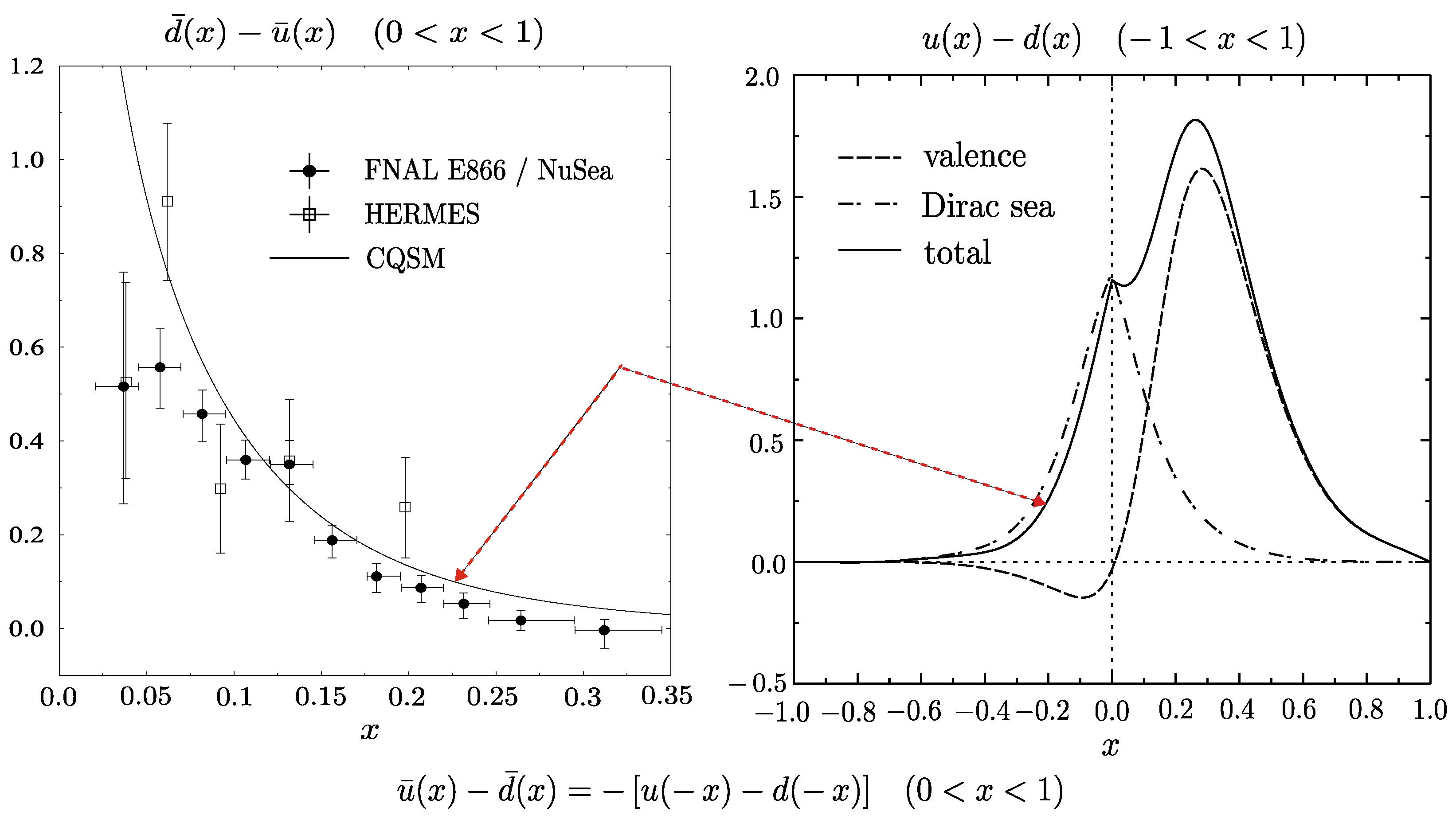
Now we are in a position to compare the basic predictions of the CQSM for the twist-2 PDFs evolved to a high energy scale with the corresponding experimental data. Shown in Figure 7 are the experimental data by the HERMES group [38] and the FNAL E866/NuSea group [39], which clearly show the flavor asymmetry of anti-quark distribution in the proton. Undoubtedly, the -quark distribution dominates over the -quark distribution in the proton. It is known that this flavor asymmetry of the sea-quark distributions can be explained as a combined effect of the meson clouds and the asymmetry of the numbers of the u-quark and d-quark inside the proton. (See review [40] for a more detailed explanation.) In fact, the following virtual dissociation processes are expected to occur in the proton:
Taking account of the quark contents of the pions as
one first realizes that the emission of the neutral pion generates the same numbers of and pairs so that it does not contribute to the asymmetry of the numbers of and quarks. On the other hand, the processes and can generate the difference between the numbers of and pairs. Since the numbers of the parent u-quark and d-quark in the proton as the seeds of this virtual dissociation processes are two and one, this naturally explains the dominance of the -quark distribution over the -quark distribution, at least qualitatively. As one sees on the left panel of Figure 7, the CQSM reproduces fairly well the observed difference of the -quark and -quark distributions without introducing any adjustable parameters. This is not surprising, because the pion cloud effects or the pionic quark–antiquark excitation modes are automatically included into the model. Undoubtedly, such a mechanism is already incorporated in the model prediction for the distribution given at the low energy model scale. In order to confirm it, the CQSM prediction at the model energy scale is shown again on the right panel of Figure 7. As can be demonstrated from this figure, the contribution of the negative-energy Dirac-sea quarks have a positive peak with sizable magnitude. In particular, the positivity of in the negative x region means that for is negative, which in turn reconfirms that dominates over in conformity with the observation. We can say that the seed of the flavor asymmetry of the anti-quark distribution is already contained in the prediction of the CQSM given at the low energy scale.
Figure 7.
Flavor asymmetry of the unpolarized sea-quark (anti-quark) distributions in the proton. The left panel shows the prediction of the CQSM for in comparison with the experimental data by the HERMES collaboration [38] and the FNAL E866/NuSea collaboration [39]. The prediction of the CQSM here is obtained after evolving it to the energy scale of the corresponding experimental data. For the sake of comparison, the CQSM prediction at the model energy scale is re-posted on the right panel.
Next, we turn our attention to the isoscalar combination of the longitudinally polarized distribution, i.e., . Shown on the left panel of Figure 8 are the empirical data for the isoscalar longitudinally polarized quark distribution of the nucleon extracted by the COMPASS group [41,42]. This distribution function is extracted under the assumption that the deuteron is a weakly bound object of the proton and the neutron on account of the D-state probability in the deuteron wave function. Under this approximation, the function can be identified as the isoscalar unpolarized distribution function of the nucleon. The corresponding prediction of the CQSM is shown by the solid curve. One of the interesting observations is that or appears to become negative as x approaches zero, and this behavior is remarkably consistent with the theoretical prediction of the CQSM. Interestingly, this behavior is already anticipated from the prediction of the CQSM at the low energy model scale shown on the right panel of Figure 9. As one sees from this figure, the contribution of the Dirac-sea quarks to this distribution function is relatively small. Rather, the contribution of the valence quarks determines the general tendency of this distribution such that in the small x region. To avoid misunderstanding, we point out that the valence quark orbital also receives strong deformation under the influence of the hedgehog mean field. We conjecture that the above-mentioned peculiar behavior of the valence quark contribution is related to this strong deformation of the valence quark orbit.
Figure 8.
The left panel shows the longitudinally polaized distribution function of the deuteron extracted by the COMPASS group [41,42] in comparison with the prediction of the CQSM for the isoscalar longitudinally polarized distribution function of the nucleon evolved to the corresponding energy scale. Here, represents the D-state probability of the deuteron wave function. For reference, the CQSM prediction for at the low energy model scale is re-posted on the right panel.
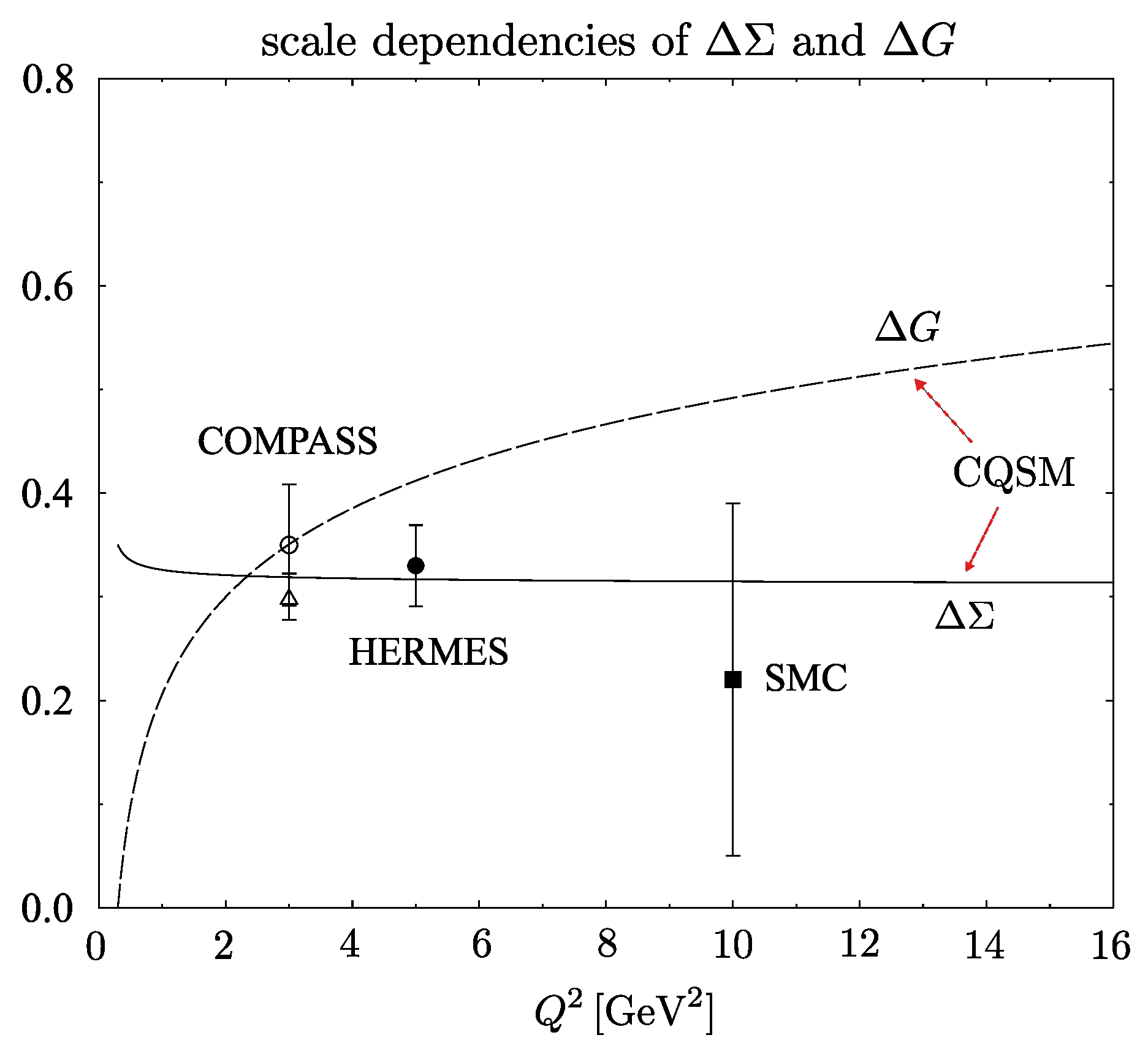
The argument above confirms that the prediction of the CQSM for the isoscalar combination of the longitudinally polarized quark distribution in the nucleon is consistent with the empirical information extracted by the COMPASS group [41,42] at least qualitatively. Incidentally, the first moment of is identified with the net quark spin fraction in the nucleon (it can be identified with the isoscalar axial-vector coupling constant of the nucleon in the gauge-invariant regularization scheme) as
Here, we explicitly show the dependencies of the quantities as well as and , which are all scale-dependent quantities. As already mentioned, the CQSM prediction for at the model energy scale gives . We try to estimate the dependence of by solving the coupled evolution equation for and at the next-to-leading order. For simplicity, the gluon spin contents at the low-energy model scale is assumed to be negligibly small and it is set to zero. Shown in Figure 9 are the scale dependencies of and . As one can see, the generally has weak scale dependence at very low energy scales. Above , it is nearly scale-independent. Interestingly, the prediction of the CQSM for [43,44] looks consistent with all the available empirical data, i.e., the old SMC data, and the newer data by the HERMES group [45] and COMPASS group [41,42]. The evolution equation predicts that, different from , the gluon spin fraction has a fairly strong scale dependence and it grows logarithmically as a function of .
Figure 9.
Energy scale dependencies of the quark spin fraction and the gluon spin fraction predicted by the CQSM [43,44], in comparison with the old fit by the SMC group [46] and the newer fits by the COMPASS group [41,42] and HERMES group [45].
Also interesting is the prediction of the CQSM for the isovector longitudinally polarized quark distribution shown in panel of Figure 4. Remembering the fact that the distribution in the negative x region can be identified with the anti-quark distribution with , we see that the CQSM predicts for the physical value of x with . Table 1 shows the integrals of the distribution functions , , , and predicted by the CQSM within the range of x designated in the upper-most row of the table. From this table, the first moments or the integrals of and within the range can be estimated as
which means that
At any rate, the CQSM predicts that the flavor symmetry of the sea-quark distributions is broken not only for the unpolarized distribution but also for the longitudinally polarized distribution in the proton.
Table 1.
The integrals of the longitudinally polarized distribution functions specified in the left-most column within the range of x designated in the upper-most row.
Before ending this section, let us briefly touch upon the CQSM prediction for the transverse momentum-dependent (TMD) distribution function of the nucleon [47]. Shown in Figure 10 is the contour plot for the isoscalar unpolarized TMD quark distribution function. The left panel stands for the quark distribution , while the right panel does the corresponding anti-quark distribution . Although it is not very easy to see only from these figures, the above predictions of the CQSM indicate that the frequently assumed factorized form with the Gaussian distribution in given as
is not necessarily justified.
Figure 10.
Contour plot of the isoscalar unpolarized transverse momentum-dependent (TMD) quark distribution functions predicted by the CQSM. The left panel represents the TMD quark distribution , while the right panel does the TMD anti-quark distribution .
To confirm the above statement more clearly, we evaluate from the theoretical distribution the average transverse momentum of quarks and anti-quarks as functions of x, which is defined by
The resultant is shown by filled squares in Figure 11. The solid curve here is a smooth fit to the above numerical results by an 8th-order polynomial. One clearly sees that the average transverse momentum square is strongly dependent on the longitudinal momentum fraction x of quarks and anti-quarks, which confirms that the frequently used assumption of factorization in the variables x and is significantly broken. Also worthy of special mention here is very unique prediction of the CQSM, which indicates that the magnitude is much larger in the negative x region corresponding to the anti-quarks. It can be demonstrated more clearly by comparing the two quantities defined below:
which represents the average transverse momentum square for quarks and anti-quarks, respectively. Numerically, we find that
which shows that the average transverse momentum of anti-quarks is sizably larger than that of quarks. We emphasize that what makes this nontrivial prediction possible is the prominent nature of the CQSM in which one is able to take account of nonperturbative deformation of the negative-energy Dirac-sea orbitals in the hedgehog mean field.
Figure 11.
The CQSM prediction for the average transverse momentum square of quarks () and of antiquarks () as a function of the longitudinal momentum fraction x.
4. Flavor SU(3) CQSM and Strange-Sea Asymmetry in the Nucleon
It is believed that the quantum nucleon state has, in general, nonzero strange quark components. To take such possibilities into account, we need a flavor SU(3) extension of the CQSM. The flavor SU(3) version of the CQSM is characterized by the following effective Lagrangian [3,48]
where
Here, stands for the octet meson fields. The last term in the parenthesis on the r.h.s of Equation (51) represents the SU(3) breaking term, which is given as
with being the mass difference between the strange quark and the non-strange quarks. In the following, we set ∼.
The basic dynamical assumptions of the flavor SU(3) CQSM are as follows:
- (1)
- The lowest energy classical solution is obtained by embedding the SU(2) hedgehog solution to the SU(3) matrix as follows:
- (2)
- Quantization of soliton rotational motion in the SU(3) collective coordinate space
- (3)
- Perturbative treatment of the SU(3) breaking term given by
The comparison with the high-energy data is carried out similarly with the case of SU(2) CQSM. We use the predictions of the CQSM for [12,13]
as initial-scale quark and anti-quark distributions given at the model energy scale . The gluon distribution functions at this low energy scale is simply set to be zero as before,
(There is some phenomenological indication, which implies that the above assumption for the longitudinally polarized gluon distribution at the above low energy scale is not so bad but the unpolarized gluon distribution at the same energy scale is not necessarily negligible.)
The greatest advantage of the SU(3) CQSM is that it can give nontrivial prediction for the asymmetry of the strange and anti-strange quark distributions in the proton. Since the net strange quark number in the proton is zero, there is a rigorous sum rule between the unpolarized strange quark distribution function and the corresponding anti-strange quark distribution :
However, this does not necessarily dictate that the distributions and are identical. In fact, in the physical picture of the meson–baryon fluctuation model due to [49,50], the following virtual dissociation process of the proton is expected to occur,
We recall here the quark contents of and , which are given as and . Note that on the r.h.s. of (57), the s-quark is contained in (baryon), while the -quark is contained in (meson). This already indicates that the distribution functions for the s-quark and the -quark need not be the same. That is, the s-quark is expected to have valence-like harder component as compared with the -quark contained in the soft meson. (To have a harder component means that it prevails in a larger x region.) This in turn indicates that the enhancement of the difference distribution at larger x.
We show in Figure 12 the prediction of the SU(3) CQSM for the distribution in comparison with the global fit by the NNPDF collaboration [51,52]. The model prediction, i.e., the enhancement of over in the larger x region, appears to be consistent with the newer fit NMPDF2.0 (and NNPDF2.1), at least qualitatively.
Figure 12.
The prediction of the SU(3) CQSM for the unpolarized distribution inside the nucleon in comparison with the global fit by the NNPDF collaboration [51,52].
A question is whether one can expect asymmetry also for the longitudinally polarized strange and anti-strange quark distributions. Many years ago, Brodsky and Ma [53] predicted the asymmetry of the distribution functions and based on the kaon cloud model of the nucleon. They argued that the strange sea in the proton is thought to be generated through the virtual dissociation process of the proton into and , . Note that here is an apparent asymmetry of the s-quark and -quark in this process. The s-quark is contained in the spin one-half baryon, i.e., , while -quark is contained in the spin zero meson, i.e., . Since the polarization of -quark in the spin zero is zero on the average, they conjectured that the polarization of -quark would be smaller than that of s-quark inside the parent proton. Shown in Figure 13 is the prediction of the SU(3) CQSM for the distributions , , and evolved to the energy scale of . The corresponding phenomenological fit for by the LSS group is also shown for reference [54,55]. One sees that the prediction of the SU(3) CQSM confirms the conjecture by Brodsky and Ma. The magnitude of the distribution is seen to be much smaller than that of . This confirms that effects of kaon cloud is taken into account automatically and effectively in the framework of SU(3) CQSM.
Figure 13.
The prediction of the SU(3) CQSM for the differences between the longitudinally polarized strange and anti-strange distributions inside the nucleon in comparison with the LSS fit for the average distribution [54,55].
Owing to the difference of the dynamical assumptions, the SU(3) CQSM gives somewhat different predictions from the SU(2) CQSM, even for some of the non-strange u-quark and d-quark distributions.
We show in Figure 14 the comparison of the predictions of the SU(3) CQSM and the SU(2) CQSM for the difference distribution in the nucleon. Also shown in this figure is the DSSV fit [56] for the same distribution given at the energy scale of . One sees that both of the SU(2) CQSM and the SU(3) CQSM predict sizable flavor asymmetry of the longitudinally polarized -quark and -quark distributions. However, the magnitude of the flavor asymmetry in the SU(3) CQSM is seen to be sizably suppressed as compared with the prediction of the SU(2) CQSM. The reason may be interpreted as follows. We recall that one of the basic theoretical postulates in the SU(3) CQSM is the collecive rotation of the hedgehog object in the flavor SU(3) space. This collective rotation is expected to drive away some of the pion clouds into the kaon clouds. This is equivalent to saying that some of the u- and d-quark components are driven away to the strange quark sector. It is thought to explain the possible reason of the reduction of the in the SU(3) CQSM as compared with that in the SU(2) CQSM, as illustrated in Figure 14. At any rate, it is interesting to see that the prediction of the SU(3) CQSM for the size of the difference distribution looks qualitatively consistent with that of the DSSV global fit [56].
Figure 14.
The comparison of the predictions of the SU(3) CQSM and the SU(2) CQSM for the differences between the longitudinally polarized -quark and -quark distributions inside the proton in comparison with the DSSV fit [56] given at the energy scale of .
Finally, we show in Figure 15 the predictions of the SU(3) CQSM for the difference and the ratio of the unpolarized -quark and -quark distributions in the proton in comparison with the latest SeaQuest fit [57] together with the past E866/NuSea fit [39]. The main difference between the newest SeaQuest data and the old E866/NuSea data for the difference distribution is its behavior in larger x region. The old E866/NuSea fit shows that the distribution changes its sign around . On the other hand, according to the new SeaQuest fit, remains positive up to the larger x range. The latter behavior was the feature expected from most effective models of the nucleon including the CQSM. In any case, the prediction of the SU(3) CQSM looks fairly consistent with the new SeaQuest fit.
Figure 15.
The prediction of the SU(3) CQSM for the difference and the ratio of the unpolarized -quark and -quark distributions inside the proton in comparison with the latest SeaQuest fit [57] and the past E866/NuSea fit [39].
A far more delicate quantity is the ratio of the - and -quark distributions in the larger x region. This is because, in the ratio at larger x, the denominator and the numerator are both very small quantities. This makes the experimental extraction of the ratio at larger x very hard. On the right panel of Figure 15, new SeaQuest fit [57] and the old E866/NuSea fit [39] for the ratio are shown together with the corresponding prediction of the SU(3) CQSM. As anticipated from the sign change of the difference distribution around , the old E866/NuSea fit indicates that the ratio becomes smaller than unity around the same value of x. On the other hand, the new SeaQuest fit shows that this ratio remains larger than unity or even becomes much larger than unity as x increases. It seems to us that this drastic discrepancy between the new and old extraction of the ratio indicates the hardness of reliable extraction of this quantity. At the present stage, we can just say that the prediction of the SU(3) CQSM lies between the new and old experimental extractions.
5. On the Gauge-Invariant Decomposition Problem of the Nucleon Spin
It has been long known that there exist two different decompositions of the nucleon spin. The one is the Ji decomposition [14], while the other is the Jaffe–Manohar decomposition [58]. The Ji decomposition is symbolically expressed as
where
Here, represents the standard covariant derivative, while and with respectively represent the contributions of the intrinsic spin and the orbital angular momentum (OAM) of quark fields. Note that the quark OAM appearing in this decomposition is the manifestly gauge-invariant mechanical quark OAMas emphasized in [59,60]. According to Ji, the total gluon angular momentum of the gluon cannot be gauge-invariantly decomposed into the contributions of the intrinsic spin and orbital angular momentum parts [14].
On the other hand, the Jaffe–Manohar decomposition is given as
where
where represents the color quantum numbers. The quark OAM appearing in this decomposition is the so-called canonical quark OAM, i.e., . It had been long believed that, in this Jaffe–Manohar decomposition of the nucleon spin, only the intrinsic quark spin part is gauge-invariant, while other three pieces are all gauge-dependent quantities. However, after Chen et al.’s paper appeared [61,62], several authors proposed the concept of gauge-invariant extension of the canonical OAM [63,64], and the belief that the canonical OAM extended in that way can be regarded as a gauge-invariant quantity became popular. (See the reviews [65,66] for the lively debate at that time.) The theoretical basis of this idea is the decomposition of the vector potential into its physical and pure-gauge component, [61,62]. An apparent problem of such an idea is that the way of decomposition of the vector potential into the two components is not unique, so there are plural possibilities of extension. Upon noticing such frustrating circumstances, Ji, Xu, and Zhao advocated the viewpoint [67] that the Chen decomposition is a gauge-invariant extension of the Jaffe–Manohar decomposition based on the Coulomb gauge [61,62], while the Bashinsky–Jaffe decomposition is a gauge-invariant extension of the Jaffe–Manohar decomposition based on the light-cone gauge [68]. According to them, since the ways of gauge-invariant extension are not unique, there is no need for the two decompositions to yield the same physical predictions. This makes Ji revive his longstanding claim that the gluon spin (or ) has a meaning only in the light-cone gauge, and it is not a gauge-invariant quantity in a true or traditional sense. Probably, this is a statement that captures the core of the problem. If that claim is true, however, the terminology gauge-invariant extension does not reflect the truth, because the so-extended canonical OAM and/or gluon spin are actually gauge-variant quantities. Undoubtedly, it is better to use the term gauge-covariant extension instead of the term gauge-invariant extension. The critical difference between these two terminologies will be clarified shortly.
In fact, to satisfactorily judge whether some quantity is gauge-invariant or not is a fairly hard challenge in QCD. The reason is that, to show the gauge invariance of some quantity, one must evaluate and compare the expectation values of the corresponding operator between the system eigen-states in different gauges. Unfortunately, we have no analytical tool in QCD to obtain the exact nucleon eigen-states. To gain some clear insight into this difficult problem, we proposed to consider an intimately connected but much simpler problem in quantum mechanics [69,70], that is the familiar Landau problem, which handles the quantum mechanical motion of an electron in a uniform magnetic field. The key in this investigation is the quantity called the pseudo angular momentum in the Landau electron system [71,72]. It is known that, under the presence of the uniform magnetic field directed to the z-direction, there exist three types of orbital angular momenta. In the cylindrical coordinate system with and , they are expressed as
Here, and are the familiar canonical and mechanical angular momentum operators, while is called the pseudo angular momentum operator [71,72] or the conserved angular momentum operator in the terminology of [69]. Suppose that is a gauge transformation matrix which generates the transformation of the vector potential from to . Under this gauge transformation, the mechanical OAM operator transforms gauge-covariantly, i.e.,
Interestingly enough, the pseudo OAM operator also transforms gauge-covariantly as
It can be easily demonstrated as follows. First, note that the pseudo OAM operator above can be expressed as . Here, transforms gauge-covariantly, while term is obviously intact under a gauge transformation. This means that also transforms gauge-covariantly. Also noteworthy is the following fact. In the so-called symmetric gauge choice of the vector potential , the pseudo OAM operator just reduces to the ordinary canonical OAM operator,
This implies that the pseudo OAM operator can be interpreted as a gauge-covariant extension of the canonical OAM operator based on the symmetric gauge. From the gauge-covariant transformation property of and , one might be tempted to conclude that both correspond to gauge-invariant observables. This is not true, however. There actually exists a vital difference between the mechanical and pseudo OAMs. To see it, we first recall that there are two other typical choices of gauge in the Landau problem, which are called the 1st and 2nd Landau gauges. The corresponding gauge potentials in the three gauge choices are characterized as
The eigen-states in the symmetric gauge are usually denoted as , where n is the familiar Landau quantum number, while m is the eigen-value of the canonical OAM operator or the pseudo OAM operator . On the other hand, the eigen-states in the 1st Landau gauge are represented as , where n is the Landau quantum number again, while is the eigen-value of the canonical momentum operator or the pseudo momentum operator . (We do not repeat the analogous explanation of the 2nd Landau gauge eigen-states.) The above eigen-states in the 1st Landau gauge are not normalizable states, since the corresponding wave functions in the x-direction are non-normalizable plane-wave states. However, if we replace these plane-wave states by normalizable wave-packet states, we can convert the 1st Landau gauge eigen-states into normalizable states [69]. In the following, the states are supposed to represent such normalizable states. Now, we are prepared to compare the expectation values of the mechanical OAM operator and those of the pseudo OAM operator in three different gauges. It was shown in [69] that
whereas
As anticipated, the expectation values of the mechanical OAM operator is absolutely independent of the gauge choices. In sharp contrast, the expectation values of the pseudo OAM operators turn out to depend on the choices of gauge. An important lesson learned from this analysis is that the gauge-covariant transformation property of some operator does not necessarily mean the gauge invariance of the corresponding quantity. The same can be said for the gauge-covariant extension of the canonical quark OAM operator in QCD. Despite its gauge-covariance, they are not gauge-invariant quantities in a true or traditional sense in perfect accordance with the insight shown by Ji, Xu, and Zhao [67].
Exactly the same can be said for the gluon spin operator. It is long known that there is no gauge-invariant local expression of the gluon spin operator. To resolve the inconsistency between the gauge-invariance issue and its observability, Ji reopened his longstanding claim that the gluon spin has a meaning only in the light-cone gauge, and it is not a gauge-invariant quantity in a true or traditional sense, although it is measurable in deep-inelastic-scattering processes. One might feel a small self-contradiction in this statement. This is because we know that the famous gauge principle dictates that gauge non-invariant quantities do not correspond to observables. Although most experts tend to avoid touching upon such an academic issue, we nevertheless think it is unavoidable to form a common recognition, because it concerns our final shared consensus on the gauge-invariant nucleon spin decomposition problem. A likely answer implicitly accepted by several experts of perturbative QCD would be the following. That is, the gluon spin is not a genuine observable, but it is a quasi- observable, or to put it more clearly, a theoretical-scheme-dependent observable. This is not so unconventional statement if one remembers the fact that the genuine observables in the DIS processes are the structure functions not the parton (quark and gluon) distribution functions. The latter are recognized as the quantities which depend on the choice of the regularization or factorization scheme within the framework of perturbative QCD. To avoid misunderstanding, we emphasize that, different from the gluon spin , the quark spin fraction corresponds to a direct or genuine observable. This is because it can be identified with the flavor–singlet axial charge of the nucleon in the gauge-invariant factorization scheme, and because the flavor–singlet axial charge of the nucleon can, in principle, be observed through the neutrino scatterings on the nucleon. It is not the case for the gluon spin, however. The ultimate reason is that there exist no external electroweak currents, which directly couple to the flavor–blind gluon fields.
6. Nucleon Generalized Form Factors and Ji’s Angular Momentum Sum Rule
As is well-known, the electromagnetic form factors of the nucleon are defined as a non-forward nucleon matrix element of the electromagnetic current as
where , and and , usually denoted as and , correspond to the familiar Dirac and Pauli form factors of the nucleon. These electromagnetic form factors can be extracted through elastic scatterings of the electron from the target nucleon. On the other hand, the so-called generalized form factors of the nucleon are defined as a non-forward nucleon matrix element of the 2nd rank energy–momentum tensor as
(Note that the energy–momentum tensor couples to both of quarks and gluons, while the electromagnetic current couples only to quarks since gluons are electrically neutral.) Here, and are called the gravitational form factors of the nucleon. As a matter of course, it is impractical to get information about these form factors directly through the graviton–nucleon scattering process, because the gravitational interaction is far weaker than the electroweak interactions. Fortunately, these generalized form factors of nucleons are known to be related to the quantities called the generalized parton distribution functions, which can in principle be extracted through the high-energy scattering processes called the deeply virtual Compton scatterings.
The deeply virtual Compton scattering (DVCS) is the high-energy scattering process in which the initial photon is not a real photon but a virtual photon exchanged between the projectile lepton and the target nucleon. In the Bjorken limit, the DVCS scattering amplitudes are known to depend on four generalized parton distributions (GPDs), , , and , and , which contain the information about the nonperturbative quark–gluon structure of the nucleon. Here, the first two are called the unpolarized GPDs, while the last two are called the longitudinally polarized GPDs. These GPDs all depend on three kinematic variables, x, , and t. The meaning of these kinematic variables is as follows. First, t is 4-momentum transfer square of the nucleon. Second, x is the average longitudinal momentum fraction of the struck quark in the initial and final states, which is sometimes called the generalized Bjorken variable. Finally, is the difference of the longitudinal momentum fractions of the initial and final partons. It is usually called the skewness parameter.
Of our main interest here is the unpolarized GPDs and , defined as
where stands for the familiar light-like 4-vector. Here, the so-called gauge link, which is necessary for the above expression to be gauge-invariant, is omitted for simplicity. It is known that the decomposition of the nucleon spin is most conveniently made in the Breit frame. In this reference frame, the following combination of GPDs H and E naturally appear in the cross-section formulas, which we denote as and :
This decomposition precisely corresponds to the standard Sachs decomposition of the nucleon electromagnetic form factors given as
We first recall that the sum of H and E satisfy the 1st moment sum rule given as
Here, and represent the contributions of a quark with flavor q to the familiar Dirac and Pauli form factors of the nucleon. In the forward limit , their sum just gives the contribution of a quark with flavor q to the total nucleon magnetic moment (it is the sum of canonical part and the anomalous magnetic part).
More interesting to us is the 2nd moment sum rules of H and E. They are given as
Here, and respectively correspond to the momentum fraction carried by quarks with flavor q and gluons inside the nucleon as
On the other hand, and are interpreted as quark and gluon contributions to the nucleon anomalous gravito-magnetic moment (AGM). Different from and , there is no experimental information available for and at present. Nonetheless, any information for them is strongly desired. The reason is that they are the quantities which appear in the famous nucleon spin sum rule proposed by Ji [14,73], which is represented as
where
with the constraint
Here, Q denotes the sum of all active quark flavors, i.e., . ( for the two flavor case, and for the three flavor case). Then, represents the net momentum fraction carried by all the quarks in the nucleon. On the other hand, represents the momentum fraction carried by the gluon in the nucleon. The equation is nothing but the familiar longitudinal momentum sum rule of the nucleon, while the relation gives the consistency condition for the Ji’s sum rule to hold. Since the momentum fractions and are empirically well-determined by now, we realized that is only one unknown parameter in Ji’s nucleon spin sum rule.
Because of the hardness of the experimental GPD analyses, we do not have any reliable empirical information about or yet. However, there are some theoretical challenges in estimating their magnitudes, based on the lattice QCD simulations and also based on the CQSM. It is very interesting to compare the predictions of these two theoretical analyses. Unfortunately, the estimates within the Lattice QCD are given only for fairly large (fictitious) pion mass and the chiral extrapolation to the physical pion mass seems to have fairly large uncertainties. In view of these circumstances, we tried to modify the effective Lagrangian of the CQSM to include the arbitrary pion mass parameter in the following manner [43,44]:
where
The strategy is that, after obtaining self-consistent soliton solutions with several values of , we subsequently evaluate desired nucleon observables with the use of these solutions.
The left panel of Figure 16 shows the pion mass dependence of predicted by the SU(2) CQSM [43,44]. Remember that the value of is related to the anomalous magnetic moments of the nucleon as , where and stand for the anomalous magnetic moments of the u-quark and the d-quark, while and represent the anomalous magnetic moment of the proton and the neutron, respectively. It is known that this isoscalar combination of the nucleon anomalous magnetic moment takes a small negative value as . The predictions of the CQSM seem qualitatively consistent with this observation. On the other hand, the right panel of the same figure shows the pion mass dependence of predicted by the LHPC and QCDSF lattice QCD groups [74,75] in comparison with the predictions of the CQSM. The CQSM predicts that is identically zero independently of the pion mass. It is only natural, since there is a general constraint such that and the CQSM contains no explicit gluon degrees of freedom, thereby indicating that is identically zero in this effective quark model. Note, however, that the lattice QCD simulations carried out at larger pion masses also predict a fairly small value of , although it is uncertain at the present stage whether this tendency persists even down to the physical pion mass around . In any case, it should be kept in mind that, once the value of or is known, one can decompose the net nucleon spin of one-half into the sum of the total quark angular momentum and the total gluon angular momentum . Besides, one important piece of information obtained from the analysis in the present section is that the magnitude of or is likely to be fairly small. In the following section, further decomposition of the net nucleon spin will be tried by making use of this observation, together with some other empirical information.
Figure 16.
The left panel shows the pion mass dependence of predicted by the CQSM [43,44]. On the other hand, the right panel shows the pion mass dependence of predicted by the LHPC and QCDSF lattice simulations carried out with virtually large pion masses [74,75]. Also shown there is the prediction of the CQSM for the same quantity.
7. Semi-Empirical Analysis of Nucleon Spin Contents and Their Scale Dependencies
We again start with the nucleon spin sum rule of Ji given as [14,73]
where
with the constraint and . As is well-known, momentum fractions and are both scale-dependent quantities. An interesting observation made by Ji is that and obey exactly the same evolution equations as and do. According to him, this follows from the fact that the operation which makes the angular momentum operator different from the energy momentum operator does not change the short distance singularity of the operator. (See [14] for more detail.) The solution of this (coupled) evolution equation for or is extremely simple at the leading order (LO) of the perturbative renormalization group scheme. It is given as
with being the number of active quark flavor. In our actual analysis below, we take account of the scale dependencies of the relevant quantities by using more involved evolution equations for the momentum fractions at the next-to-leading order (NLO) by making use of the previously mentioned fact that (and also obey the same evolution equations. As initial data of evolution, we use the MRST fit for the quark and gluon momentum fractions [76] given at ,
Since the lattice QCD indicated that is likely to be small, let us simply assume that
This is a drastic postulate, but we nevertheless think it useful to gain valuable insights into the scale dependencies of the nucleon spin contents. In order to further decompose the total angular momentum of quarks and gluon into the contributions of intrinsic spins and orbital angular momenta, we adopt the frequently used definitions of the quark and gluon orbital angular momentum (OAM) given by
It is very important to recognize that the net quark OAM defined as above is the mechanical OAM not the canonical OAM. Also important to recognize is the fact that the gluon OAM defined as above is not the canonical gluon OAM appearing in the Jaffe–Manohar decomposition but it is the sum of the canonical gluon OAM and what we call the potential angular momentum [59,60]. We emphasize that the potential angular momentum is present only for gluons bound in the nucleon.
Now let us estimate the nucleon spin contents, especially their scale dependencies based on the strategy as follows. First, we recall that, as for the quark and gluon momentum fractions, and , MRST2004 fit [76] and CTEQ5 QCD fit [77] give almost the same numbers in the range between and . For example, their fits give
To get full decomposition of the nucleon spin, we also need the information for the quark and gluon spin fractions, and , at . We already know that is almost scale-independent at these energy scales and that is around 0.3. The value of around is not still reliably determined. There are some global fits at . For example, the DSSV collaboration gives [56]. On the other hand, the recent lattice calculation at the physical pion mass by the CLQCD collaboration predicts at [78]. As a trial choice for the present qualitative analysis, we choose
Now, under the approximation that and , the values of and , as well as and , are nonetheless prepared at . We also know the coupled NLO evolution equation for and also for . After solving these evolution equations, we are able to know the values of these four quantities at arbitrary . This also enables us to get the values of the net quark and gluon OAMs at any from the relations
(One should keep in mind the caution given below in Equations (101) and (102) as to the physical meaning of these OAMs.)
We show in Figure 17 the scale dependencies of the nucleon spin contents. The left panel shows the scale dependencies of the four pieces of the net nucleon spin multiplied by two, i.e., , , , and . One sees that both the gluon spin and the gluon OAM have fairly strong scale dependencies even at high energy scales. This means that to talk about the decomposition without specifying the energy scale tends to cause confusion. On the other hand, on the right panel of the same figure, the net gluon angular momentum is shown without decomposing it to its spin and OAM parts. In that case, we see that the scale dependence of the three quantities , , and are moderately weak, at least above . As pointed out in Section 5, in the original nucleon spin decomposition of Ji, he stated that the net gluon angular momentum cannot be gauge-invariantly decomposed into its intrinsic spin part and the OAM part. Whether this fact has some relation or not with the novel observation obtained through the comparison of the left and right panels of Figure 17 is a puzzling question.
Figure 17.
The left panel shows the scale dependencies of the four pieces of the nucleon spin multiplied by two, i.e., , , , and . On the other hand, on the right panel, the net gluon orbital angular momentum is shown without decomposing it into the spin and OAM components.
8. Summary and Outlook
The CQSM is a unique model of baryons, which has an intimate connection with the Skyrme model probably with wider popularity. Although the former is an effective quark theory while the latter is an effective meson theory, they share a lot of common features. For instance, the classical pion field configuration of the hedgehog shape in the Skyrme model plays the role of a mean field for quarks in the CQSM. The collective quantization of a symmetry-restoring rotational motion of the hedgehog object is also a common basic ingredient in both models. Despite these strong similarities, a conspicuous difference between the two theories was discovered already in the study of familiar low-energy observables of the nucleon. It is a novel correction, or more concretely, the 1st-order rotational correction to some observables like the isovector axial-vector coupling constant of the nucleon, which was found to exist within the framework of the CQSM but is absolutely missing in the scheme of the Skyrme model. Undoubtedly, this correction is an important key factor that makes the predictions of the CQSM more quantitative than those of the Skyrme model.
The superiority or wider applicability of the CQSM over the Skyrme model becomes much clearer if the object of study is extended from the low-energy observables to the internal partonic structure of the nucleon or any baryons. Since the parton distribution functions reflect the non-local light-cone correlation between quarks (and gluons) inside the nucleon, there is no way to handle them within the framework of effective meson theories like the Skyrme model. In contrast, this is just the place where the potential power of the CQSM as an effective quark model of baryons manifests itself. In fact, we have demonstrated that the CQSM can explain almost all the characteristic features of the various types of quark distribution functions of the nucleon. Among others, worthy of special mention is the fact that the CQSM predictions for the flavor asymmetry of both the unpolarized and longitudinally polarized sea-quark (anti-quark) distributions are remarkably consistent with the empirical information obtained from the analyses of the high-energy deep-inelastic scatterings.
On the other hand, a weakness of the CQSM is that it does not contain explicit gluon degrees of freedom, which means that the model is unable to give any meaningful predictions for the gluon distribution functions aside from the components incorporated through the perturbative QCD evolution. To overcome this weakness of the effective quark model, the numerical simulations within the lattice QCD have long been hoped for as the most promising candidate. In the past, the parton distribution functions could not be handled within the framework of the lattice QCD, since the necessary light-cone quark–quark correlations cannot be handled within this framework. However, a breakthrough has been made by the advent of the so-called large momentum effective theory by Ji and collaborators [79,80]. In this framework, one first considers the quasi-parton distribution functions, the evaluation of which requires to handle the space-like quark–quark correlations instead of the light-cone correlations. After that, the desired genuine parton distribution functions are constracted from the quasi-parton distributions by means of the sophisticated matching procedure via the large momentum nucleon states. Based on this strategy, there already exist several challenges to evaluate not only the parton distribution functions but also the generalized parton distribution functions [81,82,83,84]. At the present stage, however, what is mostly calculated are the so-called quasi parton distribution functions, not the genuine parton distribution functions. To obtain the genuine parton distribution functions from the quasi-parton distribution functions, one is required to carry out the sophisticated matching procedure [79,80]. It is not necessarily clear whether this matching procedure has already been carried out at the fully satisfactory level or not. Besides, we are not completely sure whether the effects of pionic quark–antiquark excitation modes inside baryons are taken into account at the lattice QCD simulations carried out up to now, even though all such effects are in principle believed to be incorporated automatically into the simulations within the lattice QCD framework. In light of this situation, we believe that the flavor-asymmetries of the sea-quark distributions will be an important touchstone of whether the theoretical predictions of the lattice QCD have already reached a fully realistic level or not.
Funding
This research received no external funding.
Data Availability Statement
The original contributions presented in this study are included in the article. Further inquiries can be directed to the corresponding author.
Acknowledgments
The author would like to express his deepest gratitude to the members of KEK Theory Center, especially to Shunzo Kumano, for many useful discussions on the generalized parton distribution functions and many other subjects.
Conflicts of Interest
The author declares no conflicts of interest.
Appendix A. Remarks on the Formally Unified Expression of the Quark and Antiquark Distributions
The familiar quark and antiquark distribution functions are functions of the Bjorken variable x taking the range . It is sometimes convenient to formally extend the domain of the variable x into the range . To explain how it works, we start with the definition of the unpolarized quark distribution function given as the nucleon matrix element of the quark bilinear operator with light-cone-separation as follows:
with . Here, the variable x is supposed to take positive values in the range . On the other hand, the unpolarized antiquark distribution is defined as
which is also given in the domain . In the above equation, is the anti-particle field of given as
where C is the familiar charge conjugation matrix, while represents the transpose of . Using the properties of the charge conjugation matrix, one can prove the identity
This identity dictates that the unpolarized quark distribution with a negative value of x is identified with the unpolarized antiquark distribution at a positive value of x. This relation is frequently used, since it helps in evaluating and understanding the behavior of the , etc.
Similarly, the longitudinally polarized quark and antiquark distributions are defined as
in the range . In this case, on account of the extra matrix, we find that
Although the fact that the quark distributions with negative x is related to the antiquark distribution with positive x is a property common to the unpolarized and longitudinally polarized distribution, one must pay attention to the above sign difference.
References
- Diakonov, D.I.; Petrov, V.Y.; Pobylitsa, P.V. A chiral theory of nucleons. Nucl. Phys. B 1988, 306, 809. [Google Scholar] [CrossRef] [Scilit]
- Christov, C.V.; Blotz, A.; Kim, H.-C.; Pobylitsa, P.; Watabe, T.; Meissner, T.; Ruiz Arriola, E.; Goeke, K. Baryons as non-topological chiral solitons. Prog. Part. Nucl. Phys. 1996, 37, 91. [Google Scholar] [CrossRef] [Scilit]
- Alkofer, R.; Reinhardt, H.; Weigel, H. Baryons as chiral solitons in the Nambu-Jona-Lasinio model. Phys. Rep. 1996, 265, 139. [Google Scholar] [CrossRef] [Scilit]
- Weigel, H. Chiral Soliton Models for Baryons; Lecture Notes in Physics; Springer: Berlin/Heidelberg, Germany, 2008; Volume 743. [Google Scholar]
- Witten, E. Current algebra, baryons, and quark confinement. Nucl. Phys. B 1983, 223. [Google Scholar] [CrossRef] [Scilit]
- Diakonov, D.; Petrov, V.; Pobylitsa, P.; Polyakov, M.; Weiss, C. Nucleon parton distributions at low normalization point in the large Nc limit. Nucl. Phys. B 1996, 480, 341–378. [Google Scholar] [CrossRef] [Scilit]
- Diakonov, D.; Petrov, V.; Pobylitsa, P.; Polyakov, M.; Weiss, C. Unpolarized and polarized quark distributions in the large Nc limit. Phys. Rev. D 1997, 56, 4069–4083. [Google Scholar] [CrossRef] [Scilit]
- Weigel, H.; Gamberg, L.; Reinhardt, H. Nucleon structure functions from a chiral soliton. Phys. Lett. B 1997, 399, 287–296. [Google Scholar] [CrossRef] [Scilit]
- Weigel, H.; Gamberg, L.; Reinhardt, H. Polarized nucleon structure functions within a chiral soliton model. Phys. Rev. D 1997, 55, 6910–6923. [Google Scholar] [CrossRef] [Scilit]
- Wakamatsu, M.; Kubota, T. Chiral Symmetry and the nucleon structure functions. Phys. Rev. D 1998, 57, 5755. [Google Scholar] [CrossRef] [Scilit]
- Wakamatsu, M.; Kubota, T. Chiral Symmetry and the nucleon spin structure functions. Phys. Rev. D 1999, 60, 034020. [Google Scholar] [CrossRef] [Scilit]
- Wakamatsu, M. Light-flavor sea-quark distributions in the nucleon in the SU(3) chiral quark soliton model. I. Phenomenological predictions. Phys. Rev. D 2003, 67, 034005. [Google Scholar] [CrossRef] [Scilit]
- Wakamatsu, M. Light-flavor sea-quark distributions in the nucleon in the SU(3) chiral quark soliton model. II. Theoretical formalism. Phys. Rev. D 2003, 67, 034006. [Google Scholar] [CrossRef] [Scilit]
- Ji, X. Gauge-invariant decomposition of nucleon spin. Phys. Rev. Lett. 1997, 78, 610. [Google Scholar] [CrossRef] [Scilit]
- Brodsky, S.J.; Roberts, C.D.; Shrock, R.; Tandy, P.C. New perspective on the quark condensate. Phys. Rev. C 2010, 82, 022201. [Google Scholar] [CrossRef] [Scilit]
- Kahana, S.; Ripka, G. Baryon density of quarks coupled to a chiral field. Nucl. Phys. A 1984, 429, 462. [Google Scholar] [CrossRef] [Scilit]
- Kahana, S.; Ripka, G.; Soni, V. Soliton with valence quarks in the chiral invariant σ-model. Nucl. Phys. A 1984, 415, 351. [Google Scholar] [CrossRef] [Scilit]
- Wakamatsu, M.; Yoshiki, H. A Chiral Quark Model of the Nucleon. Nucl. Phys. A 1991, 524, 561–600. [Google Scholar] [CrossRef] [Scilit]
- Kubota, T.; Wakamatsu, M.; Watabe, T. Chiral quark soliton model with Pauli-Villars regularization. Phys. Rev. D 1999, 60, 014018. [Google Scholar] [CrossRef] [Scilit]
- Adkins, G.S.; Nappi, C.R.; Witten, E. Static properties of nucleons in the Skyrme model. Nucl. Phys. B 1983, 228, 552. [Google Scholar] [CrossRef] [Scilit]
- Adkins, G.S.; Nappi, C.R. Skyrme model with pion mass. Nucl. Phys. B 1984, 233, 109. [Google Scholar] [CrossRef] [Scilit]
- Ring, P.; Schuck, P. The Nuclear Many-Body Problem; Springer: New York, NY, USA; Berlin/Heidelberg, Germany, 1980. [Google Scholar]
- Wakamatsu, M. How Dirac-sea quarks affect the neutron charge distribution. Phys. Lett. B 1991, 269, 394. [Google Scholar] [CrossRef] [Scilit]
- Sakai, T.; Sugimoto, S. Low energy hadron physics in holographic QCD. Prog. Theor. Phys. 2005, 113, 843. [Google Scholar] [CrossRef] [Scilit]
- Sakai, T.; Sugimoto, S. More on a holographic dual of QCD. Prog. Theor. Phys. 2005, 114, 1083. [Google Scholar] [CrossRef] [Scilit]
- Hashimoto, K.; Sakai, T.; Sugimoto, S. Holographic baryons: Static properties and form factors from gauge/string duality. Prog. Theor. Phys. 2008, 120, 1093. [Google Scholar] [CrossRef] [Scilit]
- Wakamatsu, M.; Watabe, T. The gA problem in hedgehog soliton model revisited. Phys. Lett. B 1993, 312, 184. [Google Scholar] [CrossRef] [Scilit]
- Christov, C.V.; Blotz, A.; Goeke, K.; Pobilitsa, P.; Petrov, V.; Wakamatsu, M.; Watabe, T. 1/Nc rotational corrections to gA and isovector magnetic moment of the nucleon. Phys. Lett. B 1994, 325, 467. [Google Scholar] [CrossRef] [Scilit]
- Wakamatsu, M. The gA problem in the Skyrme model and fermion-boson non-correspondence. Prog. Theor. Phys. Suppl. 1995, 120, 313. [Google Scholar] [CrossRef] [Scilit]
- Wakamatsu, M. Tracing the origin of the gA problem in the Skyrme model. Prog. Theor. Phys. 1996, 95, 143. [Google Scholar] [CrossRef] [Scilit]
- Reinhardt, H.; Weigel, H. Vacuum nature of the QCD condensates. Phys. Rev. D 2012, 85, 074029. [Google Scholar] [CrossRef] [Scilit]
- Schweitzer, P. The chirally-odd twist-3 distribution function e(x) in the chiral quark-soliton model. Phys. Rev. D 2003, 67, 114010. [Google Scholar] [CrossRef] [Scilit]
- Wakamatsu, M.; Ohnishi, Y. Nonperturbative origin of the delta-function singularity in the chirally odd twist-3 distributio function e(x). Phys. Rev. D 2003, 67, 114011. [Google Scholar] [CrossRef] [Scilit]
- Ohnishi, Y.; Wakamatsu, M. πN sigma term and chiral-odd twist-3 distribution function e(x) of the nucleon in the chiral quark soliton model. Phys. Rev. D 2004, 69, 114002. [Google Scholar] [CrossRef] [Scilit]
- Wakamatsu, M. Extraordinary nature of the nucleon scalar charge and its densities as a signal of nontrivial vacuum structure of QCD. Symmetry 2024, 16, 1481. [Google Scholar] [CrossRef] [Scilit]
- Miyama, M.; Kumano, S. Numerical solution of Q2 evolution equations in a brute-force method. Comput. Phys. Commun. 1996, 94, 38. [Google Scholar] [CrossRef] [Scilit]
- Hirai, M.; Kumano, S.; Miyama, M. Numerical solution of Q2 evolution equations for polarized structure functions. Comput. Phys. Commun. 1998, 108, 38. [Google Scholar] [CrossRef] [Scilit]
- Ackerstaff, K.; Airapetian, A.; Akopov, N.; Akushevich, I.; Amarian, M.; Ashenauer, E.C.; Avakian, H.; Avakian, R.; Avetissian, A.; Bains, B.; et al. Flavor asymmetry of the light quark sea from semi-inclusive deep-inelastic scattering. Phys. Rev. Lett. 1998, 81, 5519. [Google Scholar] [CrossRef] [Scilit]
- Hawker, E.A.; Awes, T.C.; Beddo, M.E.; Brown, C.N.; Bush, J.D.; Carey, T.A.; Chang, T.H.; Cooper, W.E.; Gagliardi, C.A.; Garvey, G.T.; et al. Measurement of the light antiquark flavor asymmetry in the nucleon sea. Phys. Rev. Lett. 1998, 80, 3715. [Google Scholar] [CrossRef] [Scilit]
- Kumano, S. Flavor asymmetry of antiquark distributions in the nucleon. Phys. Rep. 1998, 303, 183. [Google Scholar] [CrossRef] [Scilit]
- COMPASS Collaboration; Ageev, E.S.; Alexakhin, V.Y.; Alexandrov, Y.; Alexeev, G.D.; Amoroso, A.; Badełek, B.; Balestra, F.; Ball, J.; Baum, G.; et al. Measurement of the spin structure of the deuteron in the DIS region. Phys. Lett. B 2005, 612, 54. [Google Scholar] [CrossRef] [Scilit]
- COMPASS Collaboration; Alexakhin, V.Y.; Alexandrov, Y.; Alexeev, G.D.; Alexeev, M.; Amoroso, A.; Badełek, B.; Balestra, F.; Ball, J.; Barth, J.; et al. The deuteron spin-dependent structure functoin and its first moment. Phys. Lett. B 2007, 647, 8–17. [Google Scholar] [CrossRef] [Scilit]
- Wakamatsu, M.; Nakakoji, Y. Generalized form factors, generalized parton distributions, and the spin contents of the nucleon. Phys. Rev. D 2006, 74, 054006. [Google Scholar] [CrossRef] [Scilit]
- Wakamatsu, M.; Nakakoji, Y. Phenomenological analysis of the nucleon spincontents and their scale dependence. Phys. Rev. D 2008, 77, 074011. [Google Scholar] [CrossRef] [Scilit]
- Airapetian, A.; Akopov, N.; Akopov, Z.; Andrus, A.; Aschenauer, E.C.; Augustyniak, W.; Avakian, R.; Avetissian, A.; Avetissian, E.; Belostotski, S.; et al. Precise determination of the spin structure function g1 of the proton, deuteron and neutron. Phys. Rev. D 2007, 75, 012007. [Google Scholar] [CrossRef] [Scilit]
- Adeva, B.; Akdogan, T.; Arik, E.; Arvidson, A.; Badelek, B.; Bardin, G.; Baum, G.; Berglund, P.; Betev, L.; Bird, I.G.; et al. Spin asymmetry A1 and structure functions g1 nof the proton and the deuteron from polarized high energy muon scattering. Phys. Rev. D 1998, 58, 112001. [Google Scholar] [CrossRef] [Scilit]
- Wakamatsu, M. Transverse momentum distributions of quarks in the nucleon. Phys. Rev. D 2009, 79, 094028. [Google Scholar] [CrossRef] [Scilit]
- Blotz, A.; Diakonov, D.; Goeke, K.; Park, N.W.; Petrov, V.; Pobylitsa, P.V. The SU(3) Nambu-Jona-Lasinio soliton in the collective quantization formulation. Nucl. Phys. A 1993, 555, 765. [Google Scholar] [CrossRef] [Scilit]
- Sullivan, J.D. One-pion exchange and deep-inelastic electron-nucleon scattering. Phys. Rev. D 1971, 5, 1732. [Google Scholar] [CrossRef] [Scilit]
- Signal, A.I.; Thomas, A.W. Possible strength of the non-perturbative strange sea of the nucleon. Phys. Lett. B 1987, 191, 205. [Google Scholar] [CrossRef] [Scilit]
- NNPDF Collaboration; Ball, R.D.; Del Debbio, L.; Forte, S.; Gufanti, A.; Latorre, J.I.; Rojo, J.; Ubiali, M. A first unbiased global NLO determination of parton distributions and their uncertainties. Nucl. Phys. B 2010, 832, 136. [Google Scholar] [CrossRef] [Scilit]
- NNPDF Collaboration; Ball, R.D.; Bertone, V.; Cerutti, F.; Del Debbio, L.; Forte, S.; Gufanti, A.; Latorre, J.I.; Rojo, J.; Ubiali, M. Unbiased global determination of parton distributions and their uncertainties at NNLO and at LO. Nucl. Phys. B 2012, 855, 153. [Google Scholar] [CrossRef] [Scilit]
- Brodsky, S.; Ma, B.-Q. The quark–antiquark asymmetry of the nucleon sea. Phys. Lett. B 1996, 381, 317. [Google Scholar] [CrossRef] [Scilit]
- Leader, E.; Sidorov, A.V.; Stamenov, D.B. Role of higher twist in polarized deep inelastic scattering. Phys. Rev. D 2003, 67, 074017. [Google Scholar] [CrossRef] [Scilit]
- Leader, E.; Sidorov, A.V.; Stamenov, D.B. Longitudinal polarized parton densities updated. Phys. Rev. D 2006, 73, 034023. [Google Scholar] [CrossRef] [Scilit]
- de Floian, D.; Sassot, R.; Strattmann, M.; Vogelsang, W. Extraction of spin-dependent parton densities and thir uncertainties. Phys. Rev. D 2009, 80, 034030. [Google Scholar] [CrossRef] [Scilit]
- Leung, C.H.; Dove, J.; Nagai, K.; Nakano, K.; Prasad, S.; Tadepalli, A.S.; Aidala, C.A.; Arrington, J.; Ayuso, C.; Barker, C.L.; et al. inal SeaQuest results on the flavor asymmetry of the proton light-quark sea with proton-induced Drell-Yan process. arXiv 2025, arXiv:2512.17564. [Google Scholar]
- Jaffe, R.L.; Manohar, A. The g1 problem: Deep inelastic electron scattering and the spin of the nucleon. Nucl. Phys. B 1990, 337, 509. [Google Scholar] [CrossRef] [Scilit]
- Wakamatsu, M. Gauge-invariant decomposition of nucleon spin. Phys. Rev. D 2010, 81, 114010. [Google Scholar] [CrossRef] [Scilit]
- Wakamatsu, M. Gauge- and frame-independent decomposition of nucleon spin. Phys. Rev. D 2011, 83, 014012. [Google Scholar] [CrossRef] [Scilit]
- Chen, X.S.; Lu, X.F.; Sun, W.M.; Wang, F.; Goldman, T. Spin and orbital angular momentum in gauge theories: Nucleon spin structure and multipole radiation revisited. Phys. Rev. Lett. 2008, 100, 232002. [Google Scholar] [CrossRef] [Scilit]
- Chen, X.S.; Sun, W.M.; Lu, X.F.; Wang, F.; Goldman, T. Do gluons carry half of the nucleon momentum? Phys. Rev. Lett. 2009, 103, 062001. [Google Scholar] [CrossRef] [Scilit] [PubMed]
- Hatta, Y. Gluon polarization in the nucleon demystified. Phys. Rev. D 2011, 84, 041701. [Google Scholar] [CrossRef] [Scilit]
- Lorce, C. Gauge-covariant canonical formalism revisited with application to the proton spin decomposition. Phys. Rev. D 2013, 88, 044037. [Google Scholar] [CrossRef] [Scilit]
- Leader, E.; Lorce, C. The angular momentum controversy?: What’s it all about and does it matter? Phys. Rep. 2014, 541, 163. [Google Scholar] [CrossRef] [Scilit]
- Wakamatsu, M. Is gauge-invariant complete decomposition of the nucleon spin possible? Int. J. Mod. Phys. A 2014, 29, 1430012. [Google Scholar] [CrossRef] [Scilit]
- Ji, X.; Xu, Y.; Zhao, Y. Gluon spin, canonical momentum, and gauge symmetry. J. High Energy Phys. 2012, 2012, 82. [Google Scholar] [CrossRef] [Scilit]
- Bashinsky, S.; Jaffe, A. Quark and gluon orbital angular momentum and spin in hard processes. Nucl. Phys. B 1998, 536, 303. [Google Scholar] [CrossRef] [Scilit]
- Wakamatsu, M.; Hayashi, A. Physical symmetries and gauge choices in the Landau problem. Eur. Phys. J. A 2022, 58, 121. [Google Scholar] [CrossRef] [Scilit]
- Wakamatsu, M.; Kitadono, Y.; Zhang, P.-M. The issue of gauge choice in the Landau problem and the physics of canonical and mechanical orbital angular momentum. Ann. Phys. 2018, 392, 287. [Google Scholar] [CrossRef] [Scilit]
- Konstantinou, G.; Moulopoulos, K. Generators of dynamical symmetries and the correct gauge transformation in the Landau level problem: Use of pseudomomentum and pseudo-angular momentum. Eur. J. Phys. 2016, 37, 065401. [Google Scholar] [CrossRef] [Scilit]
- Konstantinou, G.; Moulopoulos, K. The “forgotten” pseudomomenta and gauge changes in generalized Landau level problems: Spatially nonuniform magnetic and temporally varying electric fields. Int. J. Theor. Phys. 2017, 56, 1484. [Google Scholar] [CrossRef] [Scilit]
- Ji, X. Off-forward parton distributions. J. Phys. G Nucl. Part. Phys. 1998, 24, 1181. [Google Scholar] [CrossRef] [Scilit]
- Hägler, P.; Negele, J.W.; Renner, D.B.; Schroers, W.; Lippert, T.; Schilling, K. Helicity dependent and independent generalized parton distributions of the nucleon in lattice QCD. Eur. Phys. J. A 2005, 24, 29. [Google Scholar] [CrossRef] [Scilit]
- Göckeler, M.; Hemmert, T.R.; Horsley, R.; Pleiter, D.; Rakow, P.E.L.; Schäfer, A.; Schierholz, G.; Schroers, W. Nucleon electromagnetic form factors on the lattice and in chiral effective theory. Nucl. Phys. B Proc. Suppl. 2004, 128, 203. [Google Scholar] [CrossRef] [Scilit]
- Martin, A.D.; Roberts, R.G.; Stirling, W.J.; Thorne, R.S. Physical gluons anf high-ET jets. Phys. Lett. B 2004, 604, 61. [Google Scholar] [CrossRef] [Scilit]
- Lai, H.L.; Hustopn, J.; Kuhlmann, J.; Olness, F.; Pumplin, J.; Tung, W.K. Global QCD analysis of parton structure of the nucleon: CTEQ5 parton distributions. Eur. Phys. J. C 2000, 12, 375. [Google Scholar] [CrossRef] [Scilit]
- CLQCD Collaboration; Zhao, D.-J.; Chen, L.; Dong, H.; Ji, X.; Liu, L.; Pang, Z.; Sun, P.; Yang, Y.-B.; Zhang, J.-H.; et al. Total gluon helicity contributions to proton spin from lattice QCD. arXiv 2025, arXiv:2512.243. [Google Scholar]
- Ji, X. Parton Physics on a Euclidean Lattice. Phys. Rev. Lett. 2013, 110, 262002. [Google Scholar] [CrossRef] [Scilit]
- Ji, X.; Zhang, J.-H.; Zhao, Y. Physics of the Gluon-Helicity Contribution to Proton Spin. Phys. Rev. Lett. 2013, 111, 112002. [Google Scholar] [CrossRef] [Scilit]
- Alexandrou, C. Parton distribution functions from lattice QCD. Few-Body Syst. 2016, 56, 621. [Google Scholar] [CrossRef] [Scilit]
- Lin, H.-W. Parton distribution functions and lattice QCD. EPJ Web Conf. 2019, 206, 01003. [Google Scholar] [CrossRef] [Scilit]
- Alexandrou, C.; Cichy, K.; Constantinou, M.; Jansen, K.; Scapellato, A.; Steffens, F. Light-cone parton distribution functions from lattice QCD. Phys. Rev. Lett. 2018, 121, 112001. [Google Scholar] [CrossRef] [Scilit] [PubMed]
- Constantinou, M.; Courtoy, A.; Ebert, M.A.; Engelhardt, M.; Giani, T.; Hobbs, T.; Hou, T.J.; Kusina, A.; Kutak, K.; Liang, J.; et al. Parton distributions and lattice-QCD calculations: Toward 3D structure. Prog. Part. Nucl. Phys. 2021, 121, 103908. [Google Scholar] [CrossRef] [Scilit]
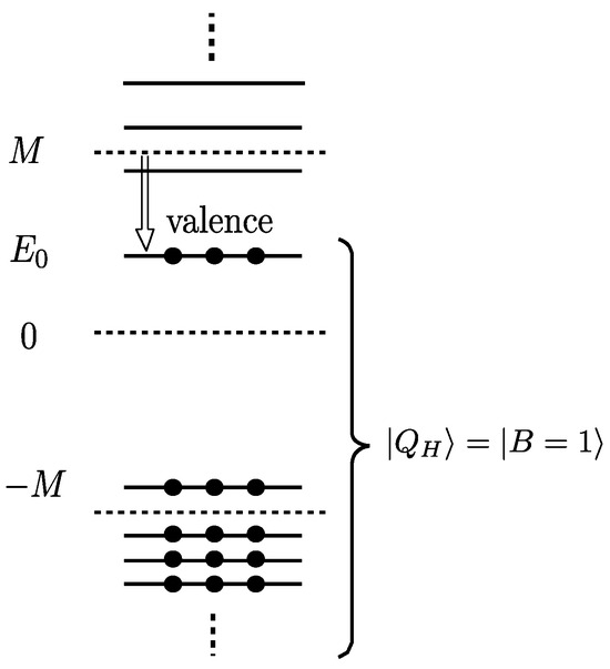
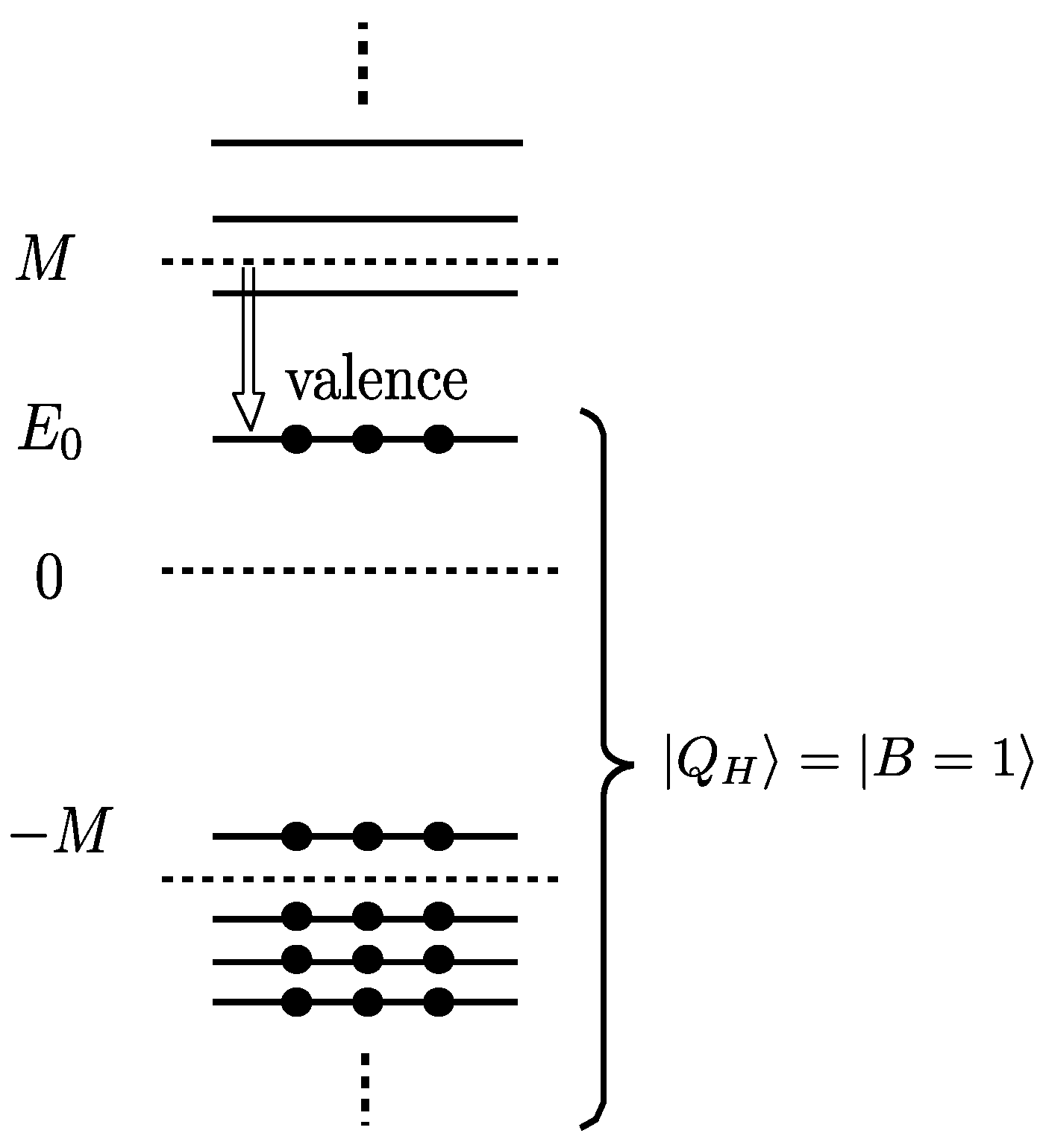
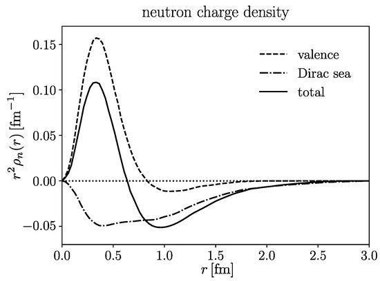
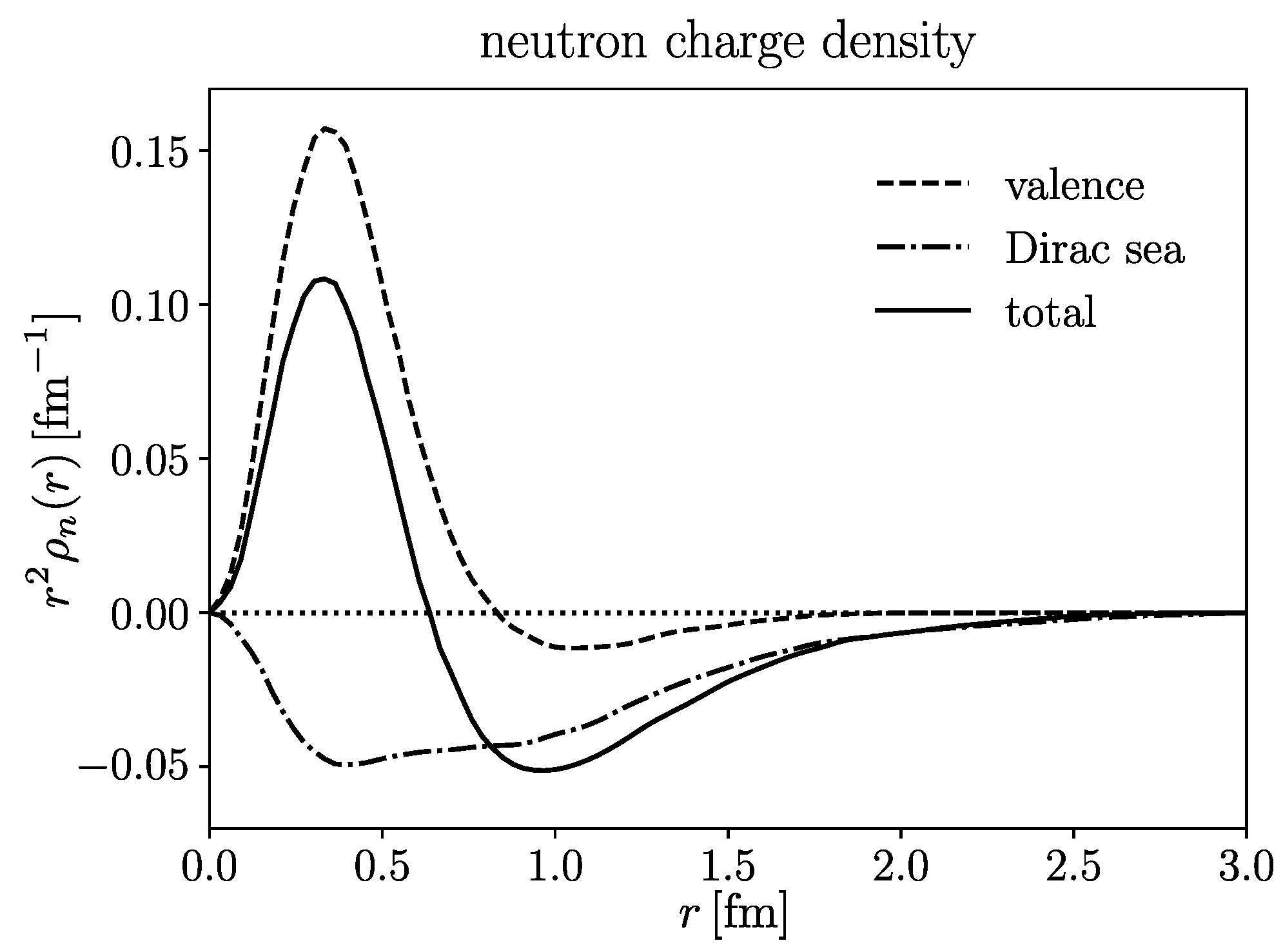
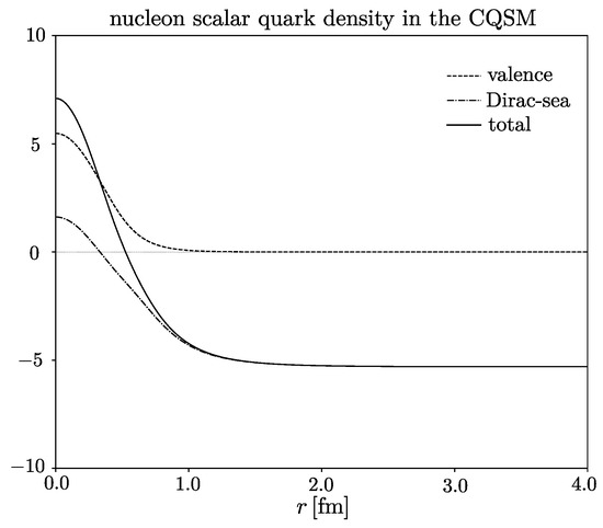
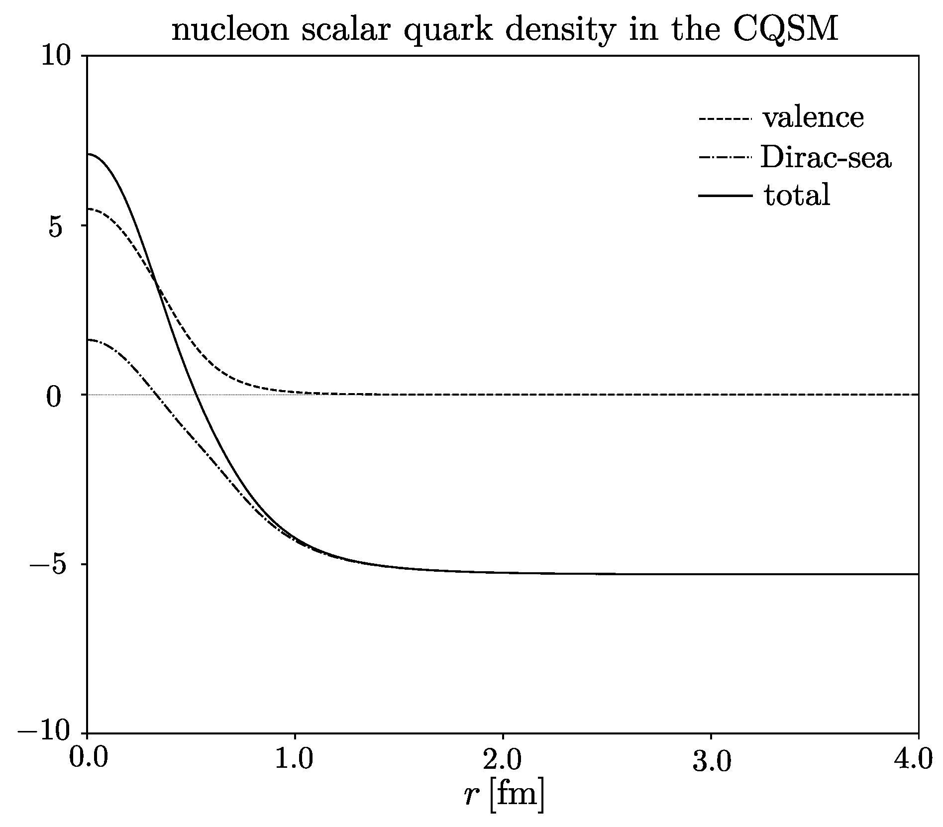
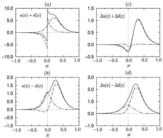
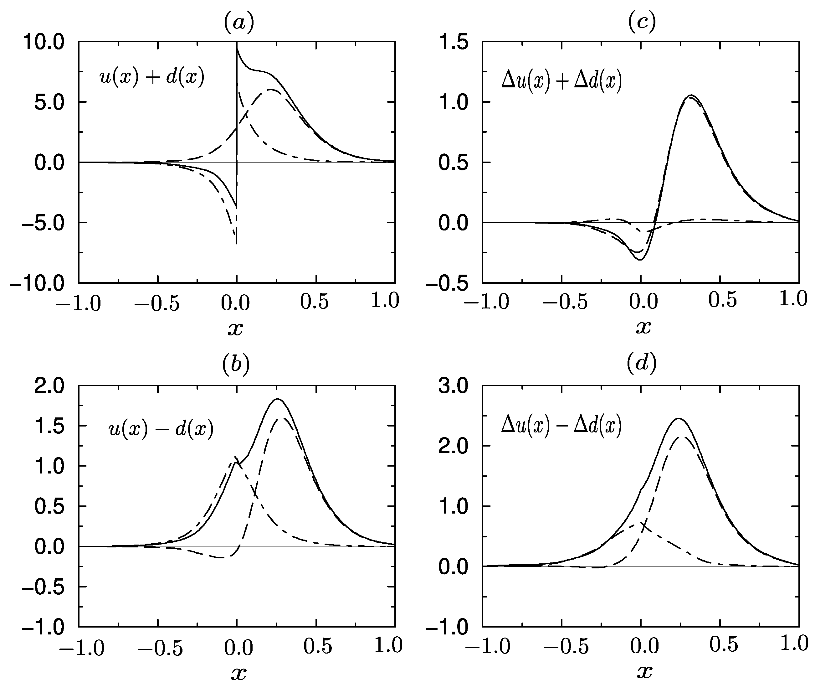
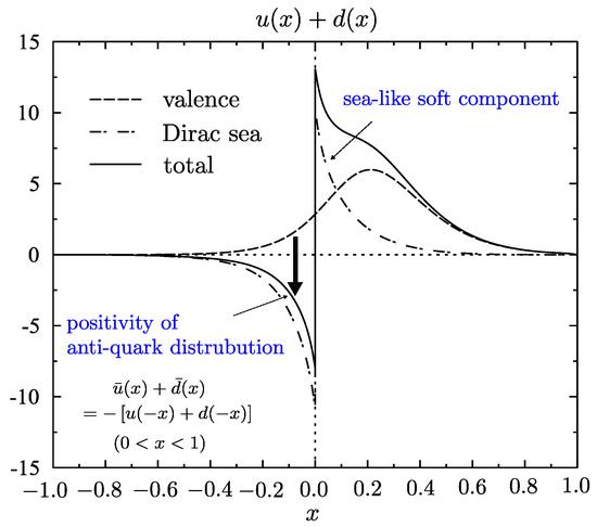
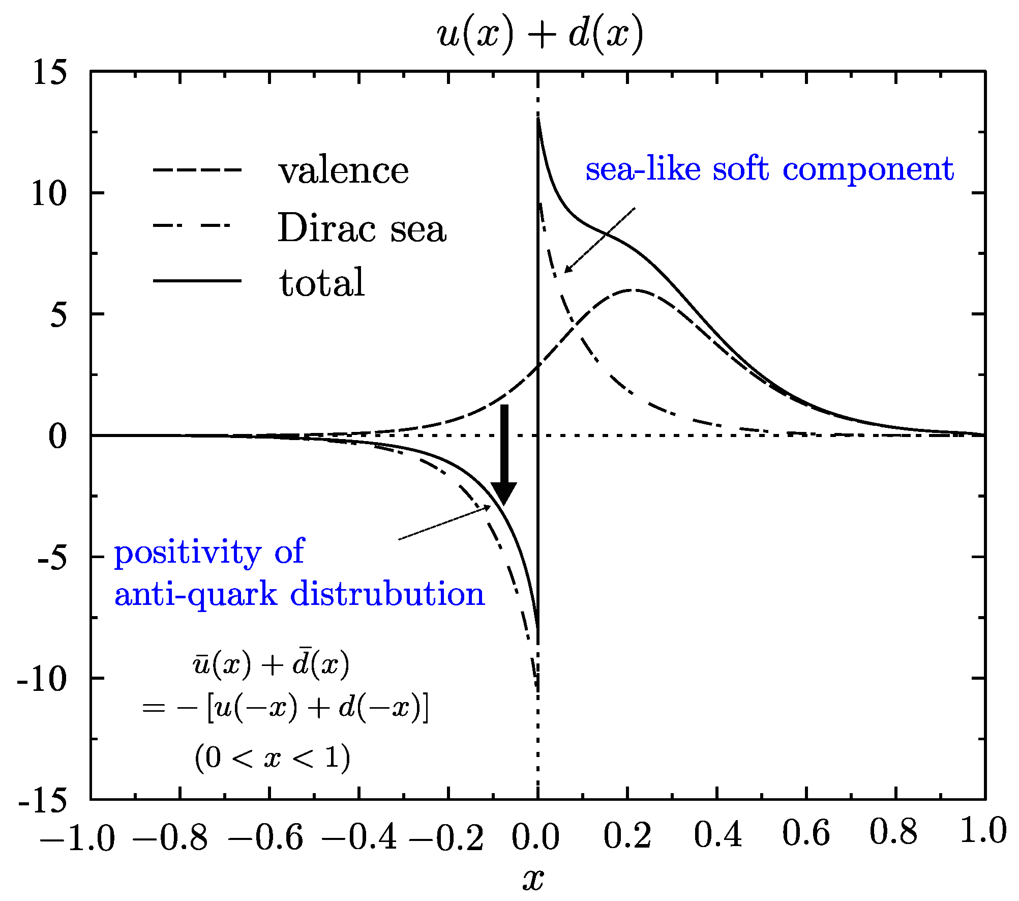
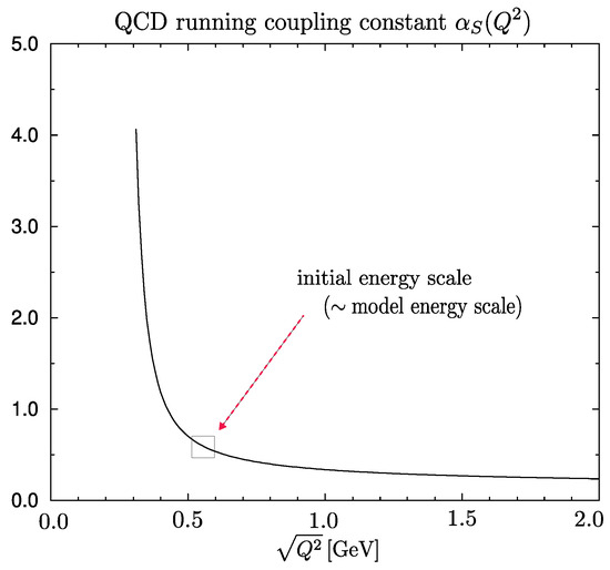
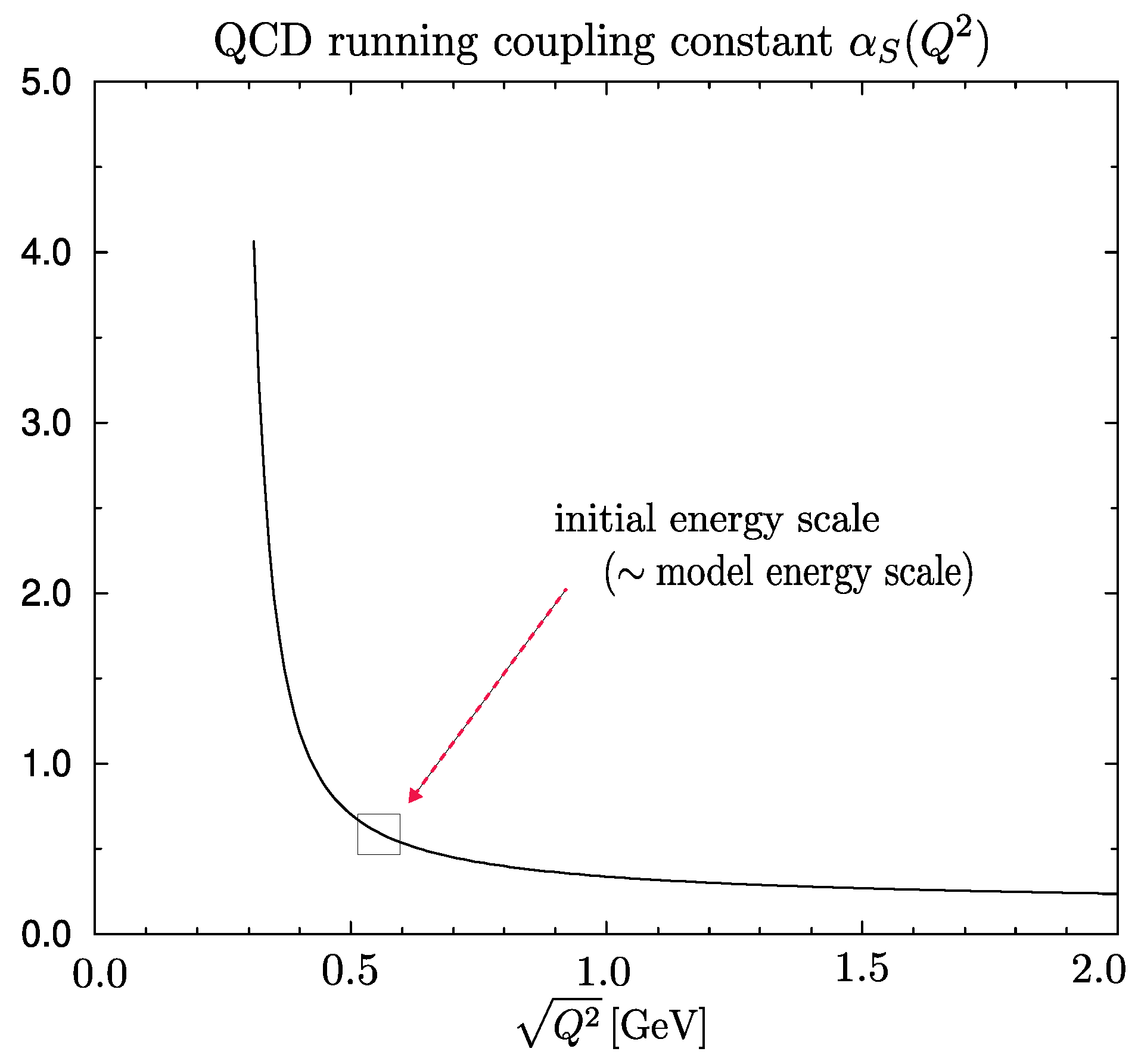
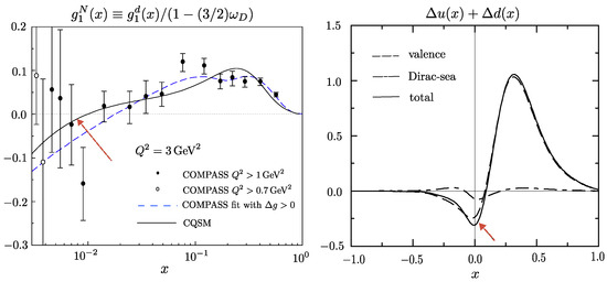
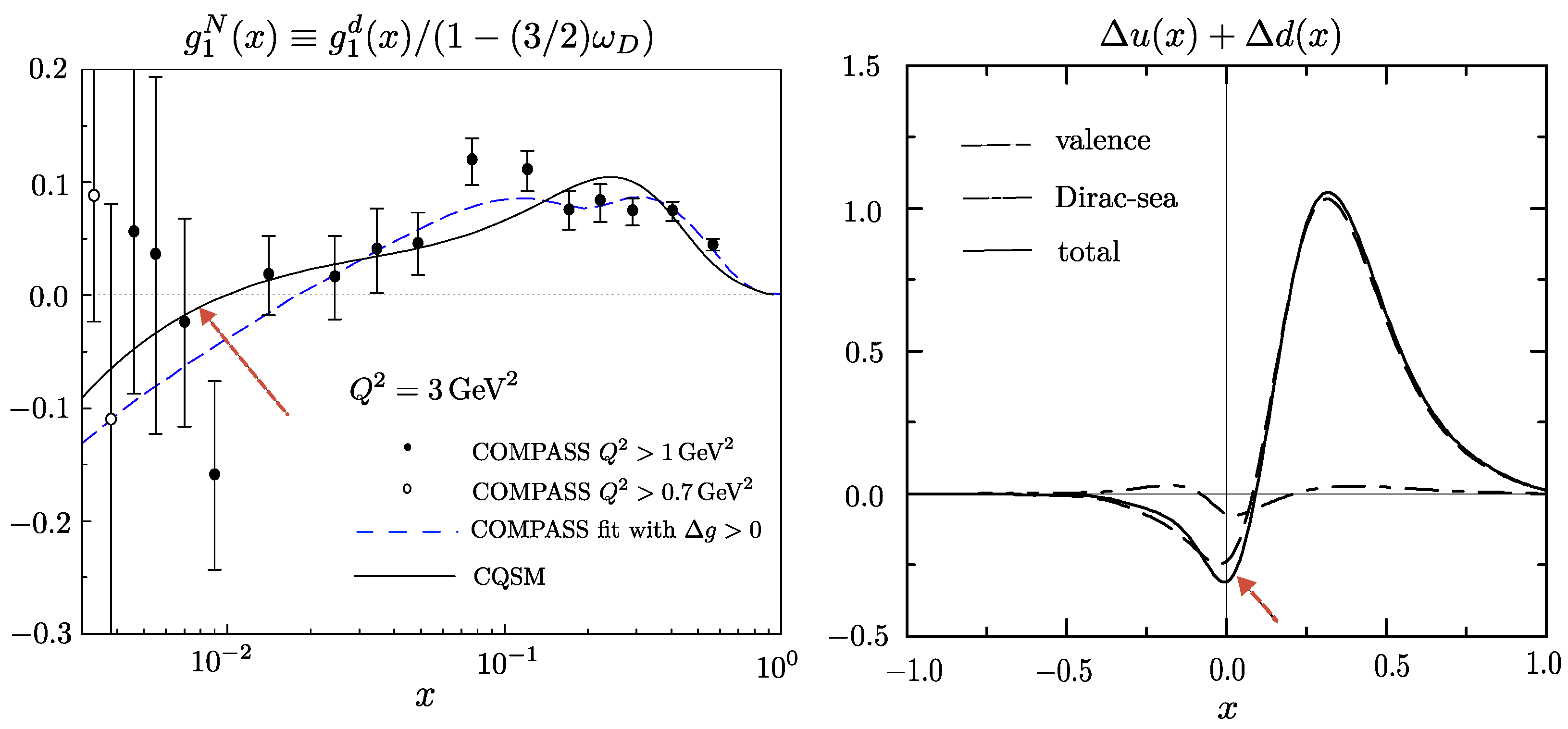
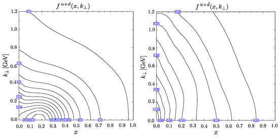
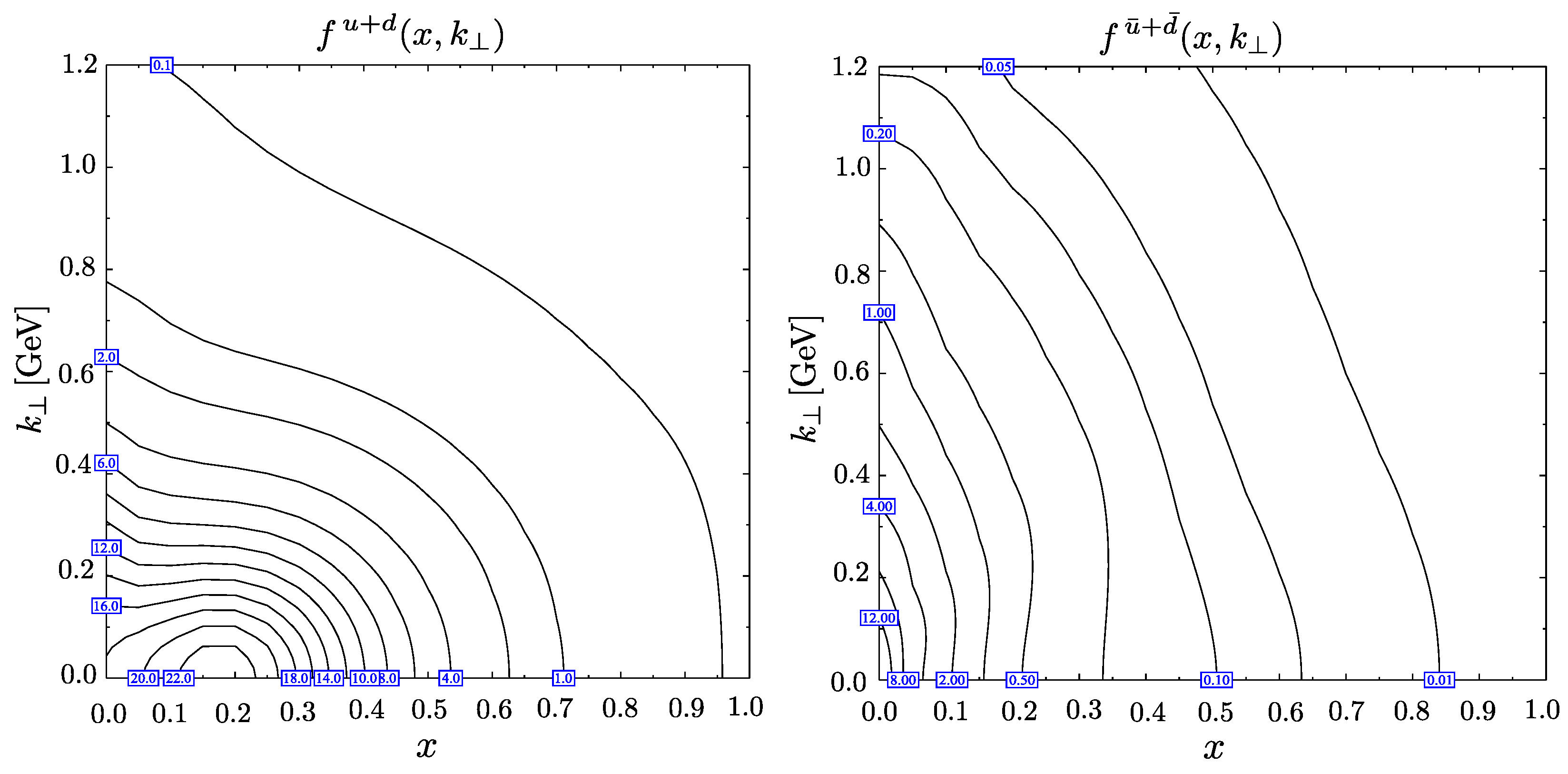
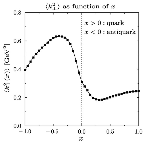
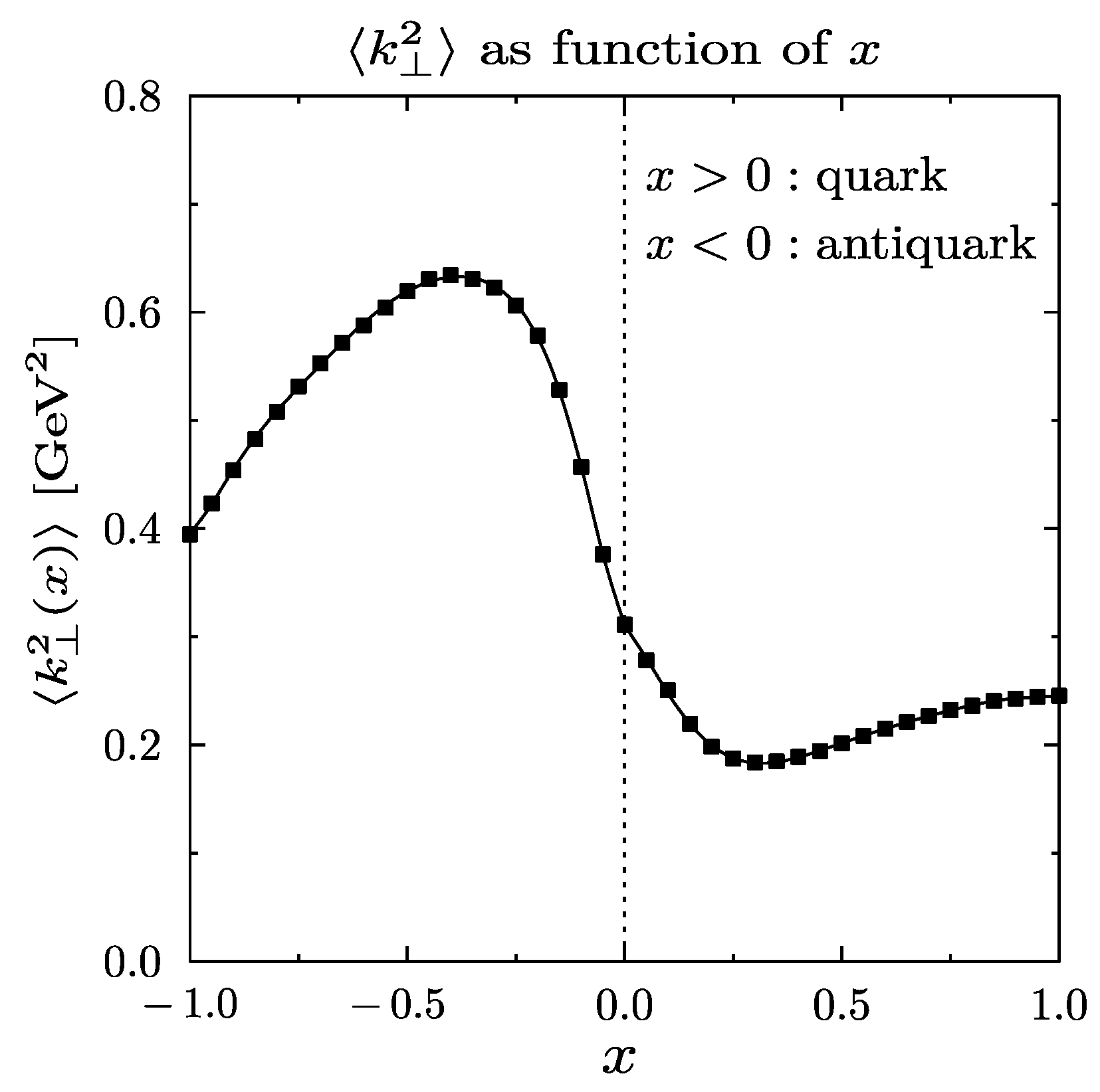
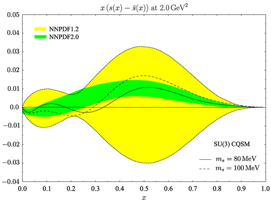
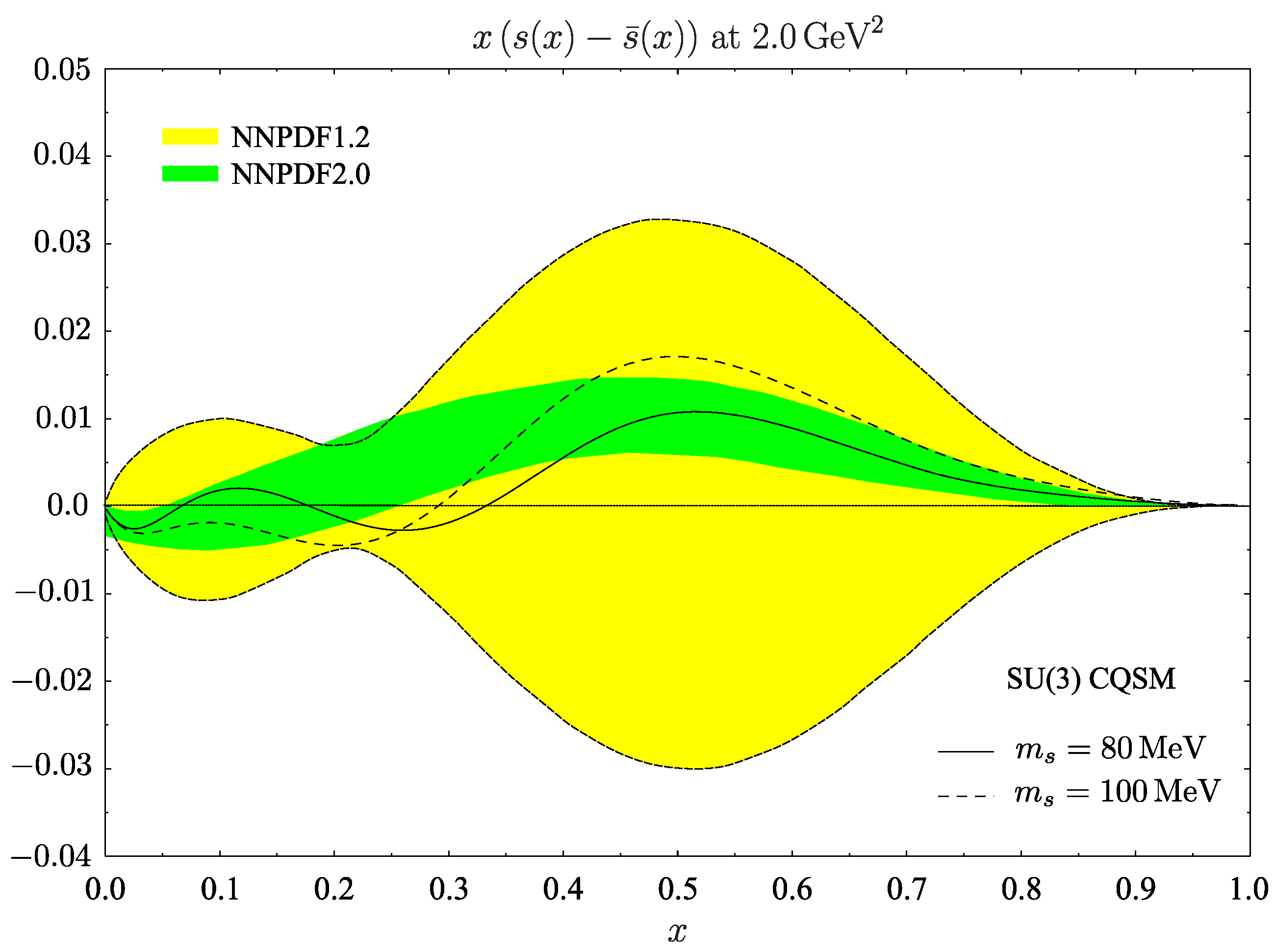
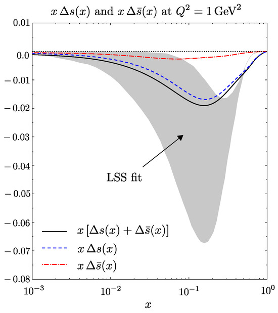
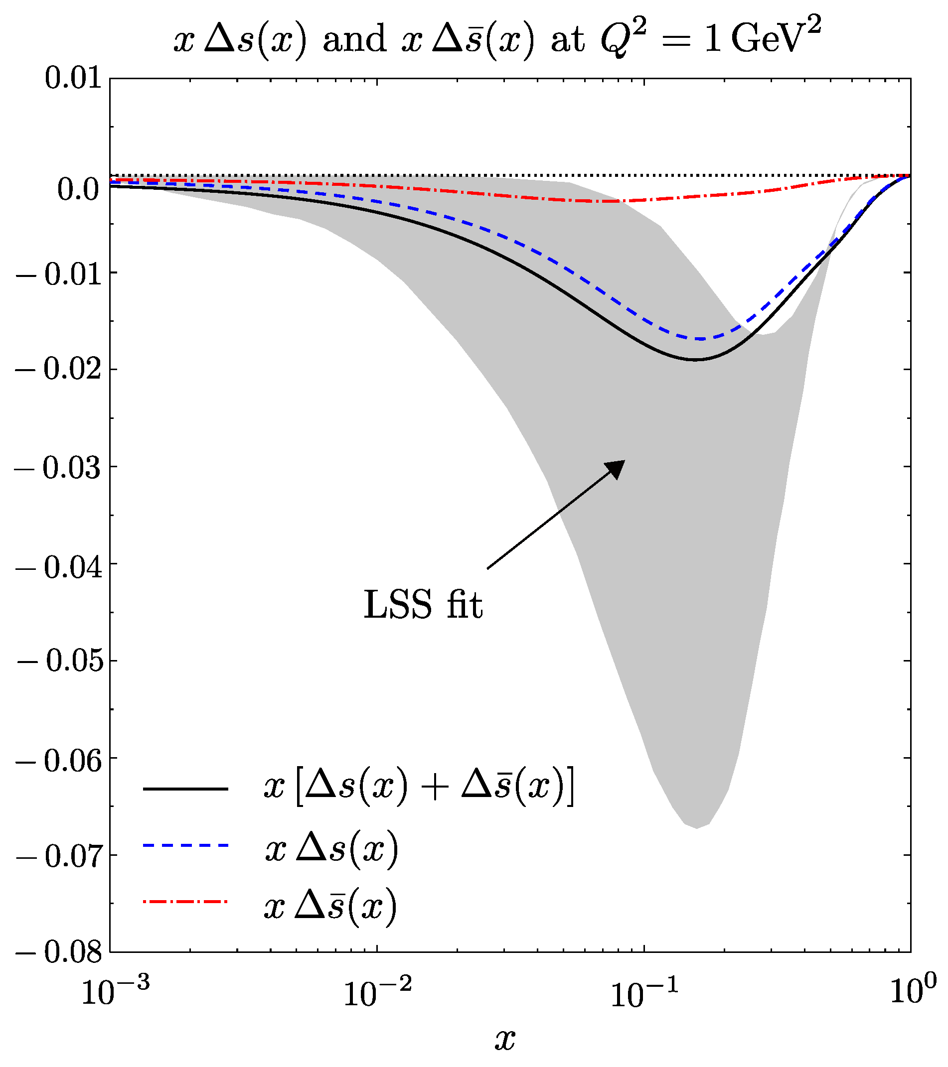
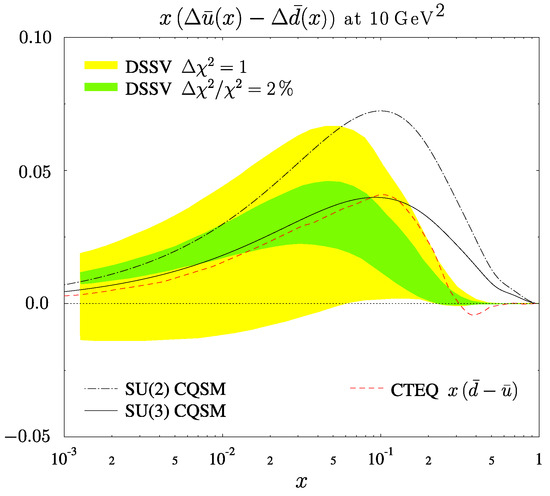
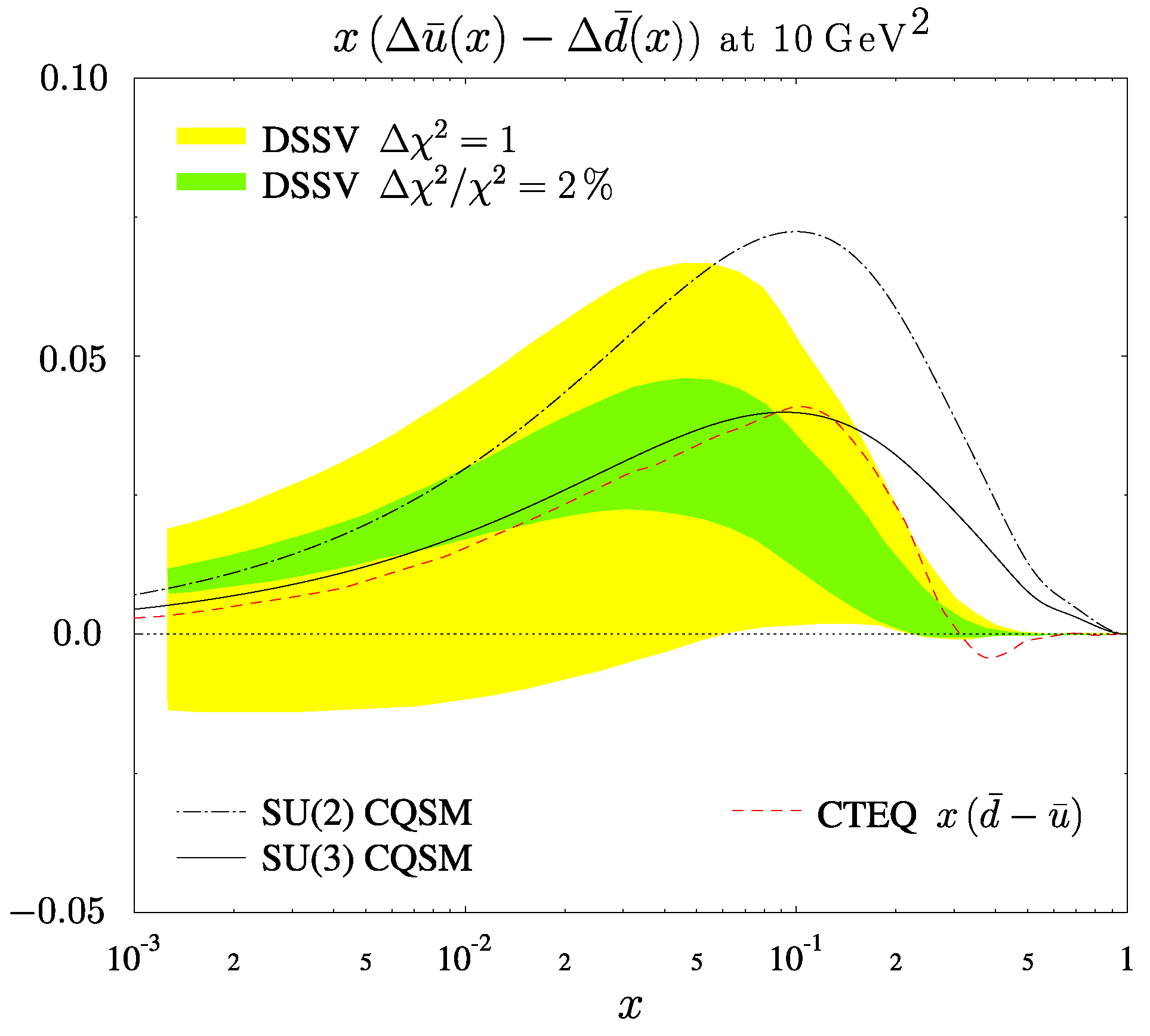
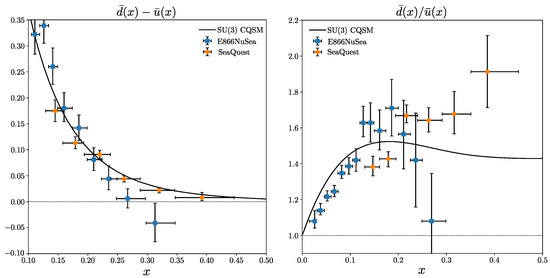
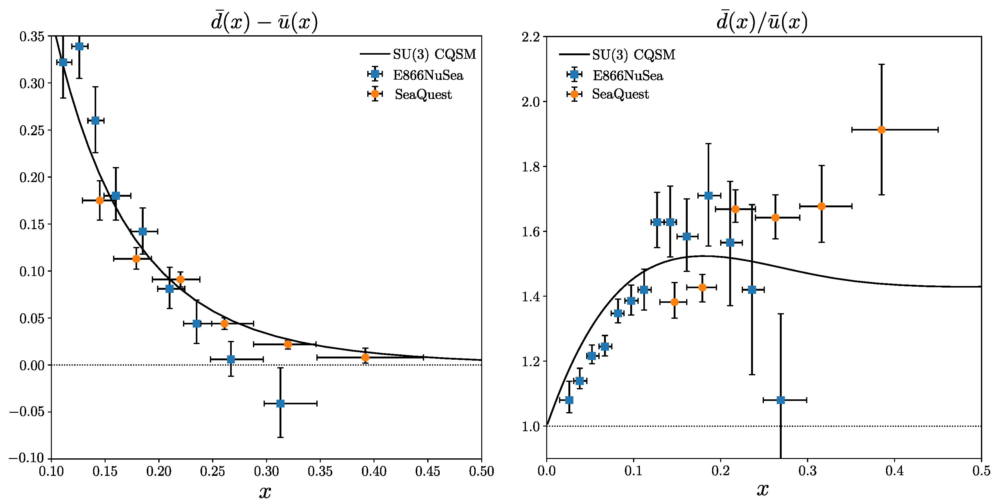
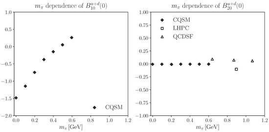
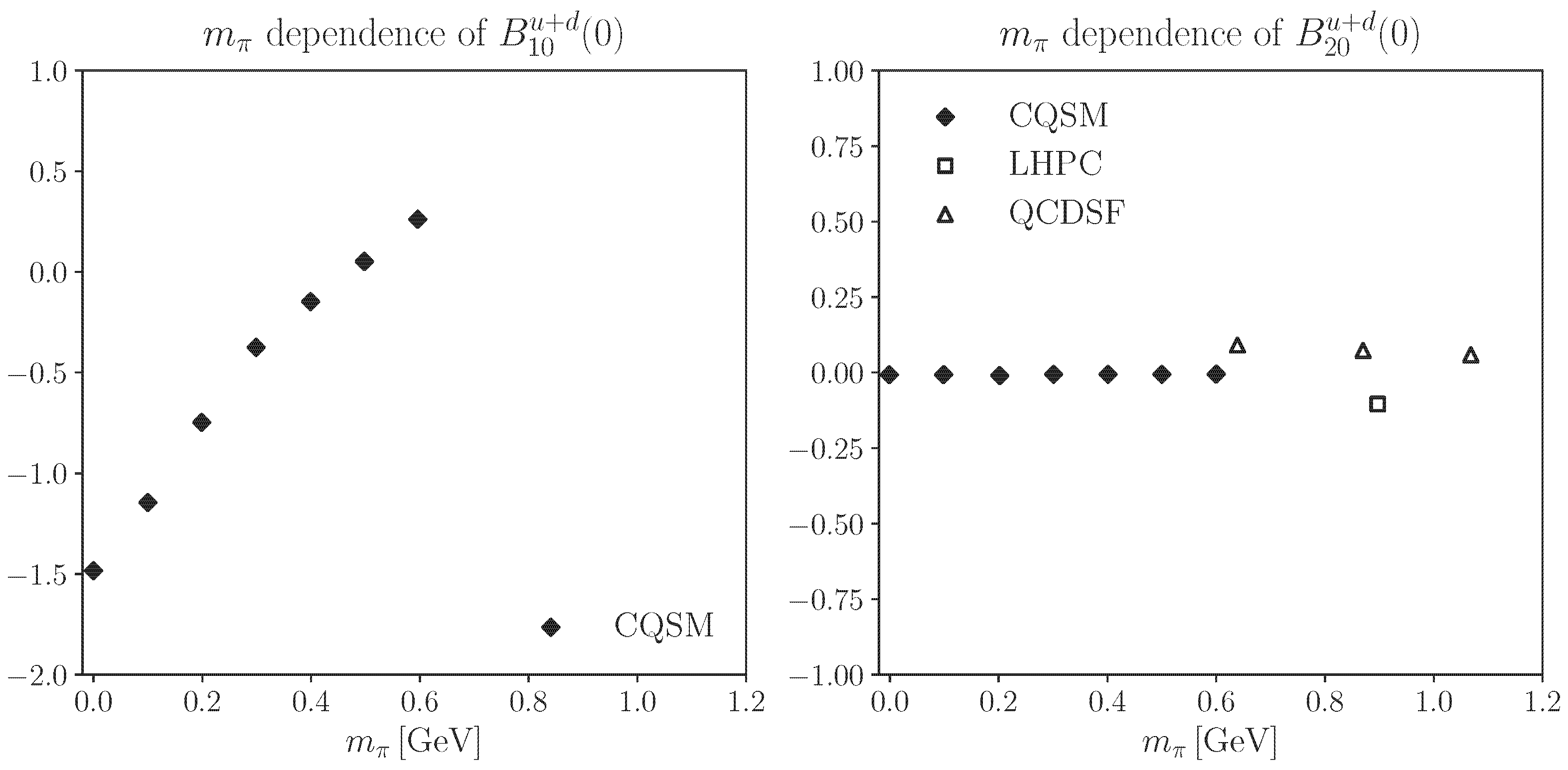
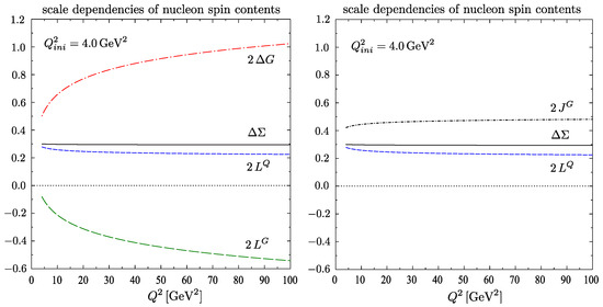
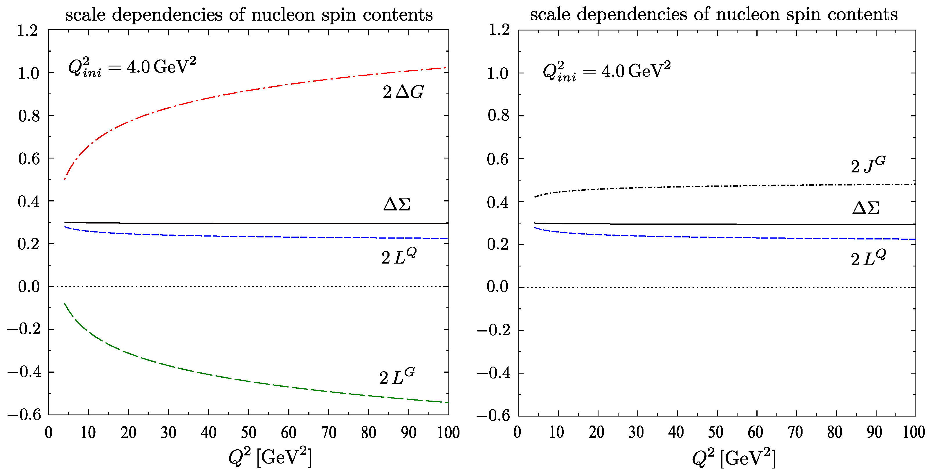

Disclaimer/Publisher’s Note: The statements, opinions and data contained in all publications are solely those of the individual author(s) and contributor(s) and not of MDPI and/or the editor(s). MDPI and/or the editor(s) disclaim responsibility for any injury to people or property resulting from any ideas, methods, instructions or products referred to in the content. |
© 2026 by the author. Licensee MDPI, Basel, Switzerland. This article is an open access article distributed under the terms and conditions of the Creative Commons Attribution (CC BY) license.