Disturbance Location-Aware Frequency Support in New Power Systems via Heterogeneous Nodal Frequency Response Modeling and Atlas-Based Gain Scheduling

Abstract

New power systems with penetration of inverter-based resources (IBRs) exhibit symmetry breaking in post-disturbance frequency, as nodal trajectories depend on disturbance location, network coupling, and heterogeneous frequency channels across synchronous generators (SGs), grid-forming (GFM) converters, and grid-following (GFL) converters with phase-locked loops (PLLs). As a consequence, relying only on aggregated center-of-inertia/center-of-frequency (COI) metrics can underestimate asymmetric local risks, including worst-node rate of change of frequency (RoCoF), worst-node nadir, and nodal frequency split. This paper proposes a disturbance location-aware coordination framework that explicitly models and balances heterogeneous active-power frequency support across the network using an electromechanical-scale state-space formulation. First, a heterogeneous nodal frequency response (HNFR) model yields an explicit state-space input–output mapping from location-specific active power disturbances to nodal frequency outputs for both electromechanical and PLL-estimated channels. Second, a reproducible signal processing protocol computes nodal RoCoF/nadir/split indices and enables large-scale location sweeping via atlas-ready matrices that are naturally parallelizable for high-performance computing. Third, a constrained allocation layer schedules heterogeneous fast frequency response subject to converter limits and finite energy constraints, supporting an atlas-based gain scheduling implementation. Case studies demonstrate that the proposed symmetry-aware design improves worst-node security and suppresses frequency split while maintaining comparable COI behavior. Under budget-matched conditions on the modified IEEE 39-bus system, the proposed allocation reduces worst-node RoCoF by 32.2% and maximum nodal frequency split by 17.8% relative to the COI-based benchmark.

1. Introduction

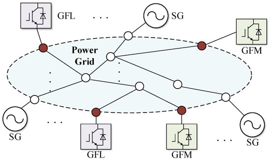
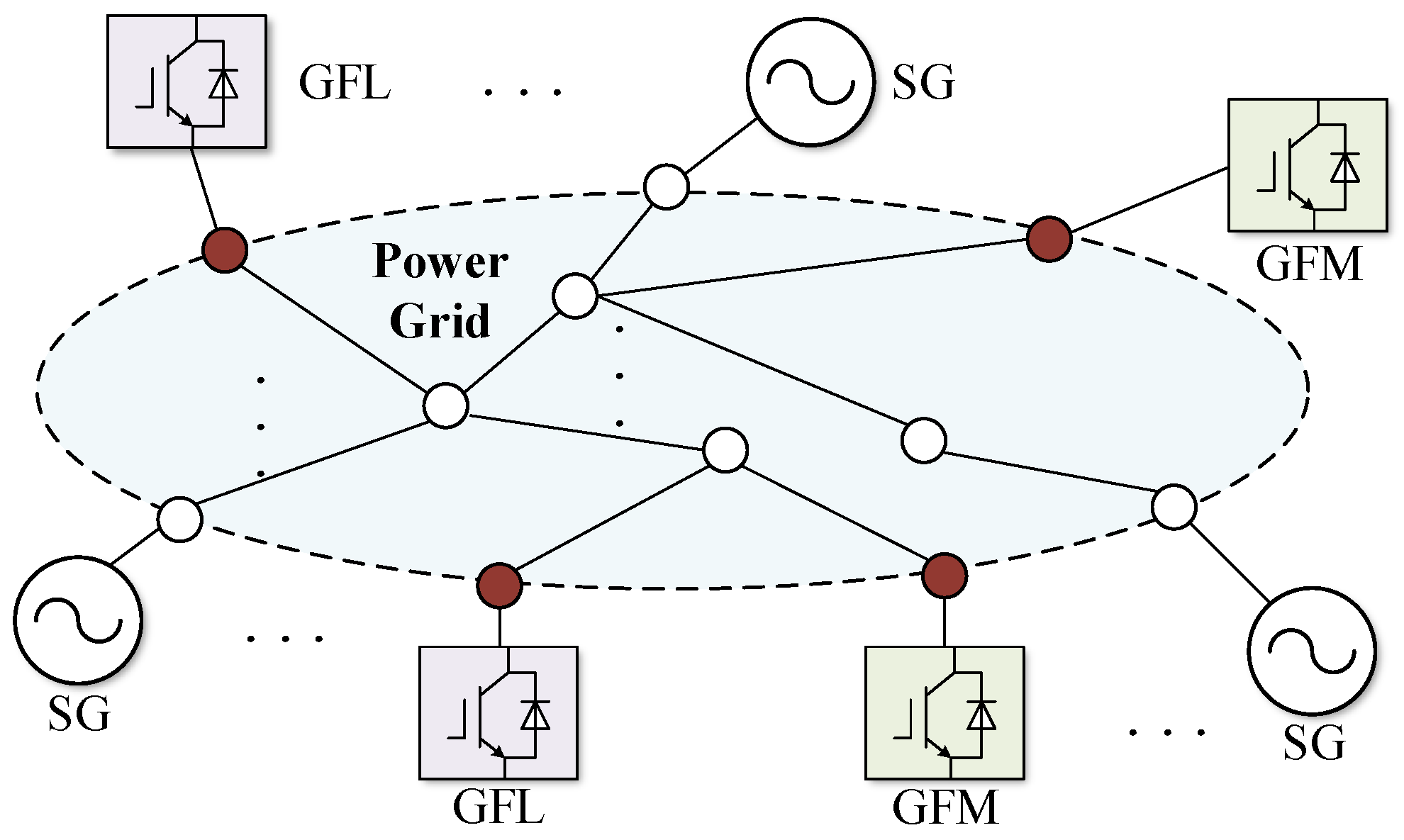
The rapid growth of inverter-based resources (IBRs) is reshaping the dynamical landscape of power systems. Under disturbances, frequency dynamics can exhibit pronounced symmetry breaking across the network. Additionally, as synchronous generators are displaced (see Figure 1), system inertia and governor-based damping decline while converter control and synchronization loops introduce new multi-timescale couplings among angle, frequency, and voltage dynamics [1,2,3,4,5]. As a result, post-disturbance frequency is no longer well-represented by a single global trajectory: nodal responses can depend strongly on disturbance location and network coupling, leading to spatially heterogeneous RoCoF/nadir and even nodal frequency splitting.

Figure 1. Diagram of an IBR-integrated power system. SG: synchronous generator; GFM: grid-forming converter; GFL: grid-following converter; IBR: inverter-based resource.

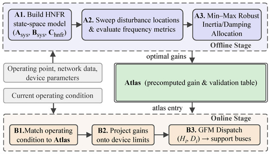
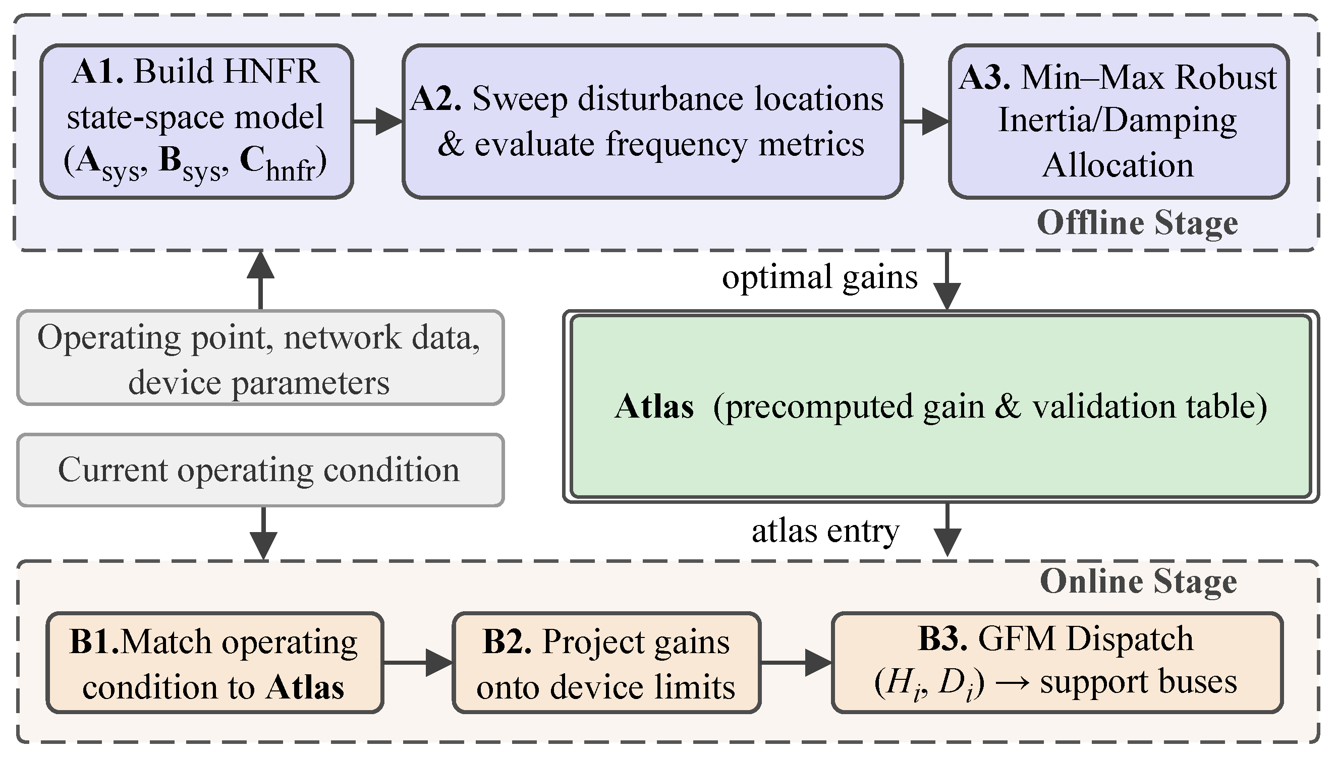
Figure 2 illustrates the end-to-end pipeline of the proposed framework. In the offline stage, the HNFR state-space model is assembled from the operating point, network data, and device parameters (step A1), the candidate disturbance location set is swept to evaluate nodal frequency security indices (step A2), and a min–max allocation layer populates an offline atlas with robust gain vectors (step A3). In the online stage, the prevailing operating condition is matched against the atlas (step B1), the stored gains are projected onto current device limits (step B2), and the resulting $(H_i,D_i)$ setpoints are dispatched to the GFM support buses (step B3). Because the atlas already hedges against all candidate disturbance locations, explicit online disturbance localization is not required.

Figure 2. Framework of the proposed atlas-based gain scheduling scheme.

Frequency security in low-inertia grids is commonly evaluated by the rate of change of frequency (RoCoF) and the frequency nadir, both of which are closely related to the available inertia and fast frequency response (FFR) capability [6,7]. In practice, operators are often concerned with worst-node risks rather than averaged behaviors, since local RoCoF and local nadir can drive protection actions and operational constraints. Moreover, in modern grids these metrics are strongly influenced by measurement and estimation chains (filtering, windowing, noise, and event detection), which motivates the use of reproducible protocols for RoCoF/nadir computation and fair comparison of control strategies [8,9,10].

A key limitation of many classical frequency studies is the reliance on aggregated indicators such as center-of-inertia/center-of-frequency (COI/COF), which includes the implicit assumption that frequency dynamics are sufficiently homogeneous across the network. Recent analytical and data-driven evidence shows that post-disturbance frequency responses can exhibit pronounced spatial disparities, with certain buses experiencing substantially larger RoCoF or deeper nadirs than those predicted by aggregated models [11,12,13,14,15,16]. Such spatial heterogeneity becomes more salient when inertia and damping are unevenly distributed and when frequency support actions are geographically concentrated.

Understanding and controlling spatial frequency behavior requires careful definitions of nodal frequency, especially when heterogeneous synchronization mechanisms coexist. While synchronous generators and grid-forming (GFM) converters are naturally associated with electromechanical frequency channels, grid-following (GFL) converters measure frequency through phase-locked loops (PLLs), for which the estimated frequency can deviate from electromechanical notions under weak-grid conditions [17,18]. This coexistence motivates unified yet channel-aware modeling frameworks that can map a location-specific active power disturbance to both mechanical frequency and PLL frequency outputs [19,20,21,22].

On the control side, the interplay between GFM and GFL inverters has attracted growing attention, particularly regarding how their parameter choices shape nodal RoCoF/nadir trajectories and stability margins. Analytical design and tuning rules have been proposed to coordinate GFM droop/inertia and GFL PLL bandwidth so as to meet frequency objectives at multiple buses rather than only at the COI [23]. Meanwhile, practical enhancements of GFL control for stiff and weak grids, comprehensive modeling comparisons for PLL-based inverters, and emerging circuit-model augmentations that better capture PLL-driven instabilities collectively highlight that weak-grid frequency behavior is inseparable from PLL dynamics and the associated modeling assumptions [24,25,26,27].

Beyond local device tuning, disturbance location-dependent frequency behavior has motivated spatiotemporal analysis tools and placement/design methodologies. Frequency distributions in systems with mixed GFM/GFL populations have been studied from both frequency domain and low-order modeling perspectives, emphasizing that frequency is not a single scalar but a field over buses and time [22,28]. This perspective aligns with spatiotemporal placement and evaluation frameworks for GFM inverters, which explicitly consider where converters are installed and how disturbances propagate through network coupling [29]. Variance-based global sensitivity analysis further provides a scalable route for quantifying locational impacts and screening influential factors under uncertainty [30].

The locational nature of frequency security also raises planning and resource allocation questions around where to place virtual inertia and FFR resources and how to tune them under device limits and finite-energy constraints. One line of work has established optimization-based placement of virtual/synthetic inertia and fast frequency response, including formulations that account for worst-case disturbance locations [31,32]. Storage-based virtual inertia placement and robust allocation of distributed energy storage systems further demonstrate that frequency security requirements can be explicitly locational and that robust methods are often needed to hedge against uncertain contingencies and operating conditions [33,34,35,36].

Complementing these planning formulations, hierarchical and distributed FFR coordination strategies prioritize electrically close resources and can reduce the reliance on centralized aggregated frequency signals, leading to improved responsiveness and scalability [37]. In addition, practical FFR designs for wind and converter-interfaced generation illustrate that fast active power support can be shaped to arrest the nadir and mitigate RoCoF, and in some settings may even offer a low-cost alternative to maintaining high synchronous inertia [38,39,40].

While the above advances provide important building blocks, two gaps remain critical for IBR-rich low-inertia grids: first, most tractable optimization and tuning approaches still rely on aggregated or homogeneous frequency models, which can underestimate worst-node risks and cannot directly quantify heterogeneous-channel incoherence; second, scalable engineering workflows that sweep disturbance locations, compute nodal RoCoF/nadir/split under a fixed protocol, and translate the resulting sensitivity patterns into deployable gain-scheduling rules remain limited [30]. These gaps motivate a disturbance location-aware framework that (i) builds an explicit heterogeneous nodal frequency response model (HNFR), (ii) evaluates nodal worst-case metrics reproducibly over disturbance location sets, and (iii) coordinates constrained heterogeneous frequency support with an atlas-based gain scheduling deployment in which the atlas serves as a pre-validated library of frequency support gain settings indexed by operating condition and designed to be retrieved online without solving a new optimization at each dispatch.

The main contributions are as follows:

• A heterogeneous nodal frequency response (HNFR) state-space model that unifies SG and GFM electromechanical frequency channels with GFL PLL-estimated frequency in a single output matrix, eliminates network algebraic variables through a reduced-order representation, and retains disturbance location as an explicit input dimension for scalable nodal frequency analysis.
• An input–output evaluation protocol that maps each candidate disturbance location to worst-node RoCoF, worst-node nadir, and nodal frequency split through a fixed signal processing chain, enabling reproducible comparison across allocation strategies.
• A robust min–max allocation formulation that schedules GFM virtual inertia and droop parameters across disturbance locations under device limits and a fixed total budget constraint, together with an atlas-based gain scheduling workflow that does not require explicit online disturbance location identification.

The remainder of the paper is organized as follows: Section 2 derives the HNFR model and the nodal frequency input–output mapping; Section 3 and Section 4 formulate the disturbance location-aware frequency support allocation problem and its tractable surrogates; Section 5 reports case studies; and Section 6 concludes the paper.

2. Heterogeneous Nodal Frequency Response Modeling for Spatiotemporal Frequency Dynamics

This section develops an HNFR framework for disturbance location-aware frequency analysis and tuning. The goal is to obtain a reproducible electromechanical-scale linearized state-space model with explicit inputs/outputs, enabling large-scale sensitivity computation and interpretable tuning rules.

Recent analytical frameworks have advanced the understanding of nodal frequency dynamics in bulk power systems. In [13], the developed natural decomposition of nodal frequency responses yielded closed-form solutions for both generation- and load-side disturbances. In [16], a reduced-order bus frequency response model was proposed to preserve spatial distribution characteristics through modal decomposition and a vibrational mechanics analogy, enabling rapid closed-form evaluation. While both frameworks provide valuable analytical insight, neither explicitly distinguishes among SG electromechanical, GFM virtual-swing, and GFL PLL-estimated frequency sources within the output space, and the latter aggregates disturbance location into an equivalent COI power perturbation. The HNFR model developed below addresses these aspects by unifying heterogeneous frequency channels within a single output matrix while retaining disturbance location as an explicit input dimension.

2.1. Modeling Scope, Frequency Definitions, and Notation

This work targets post-disturbance electromechanical frequency dynamics after fault clearing and other short-term active power disturbances under the quasi-stationary voltage assumption. Buses are partitioned into a support set $\mathcal{S}$ and following set $\mathcal{L}$ according to the dominant frequency channel; $\mathcal{S}$ includes SGs and GFM converters (voltage-source-like synchronization), while $\mathcal{L}$ aggregates GFL converters and frequency-relevant loads for which the measured frequency is dominated by PLL synchronization.

The system state vector $\mathbf{x}\in {\mathbb{R}}^{3N_S+3N_L}$ is defined as

$$\mathbf{x}=[\mathsf{\Delta }{\mathit{\delta }}_S^T,\mathsf{\Delta }{\mathit{\omega }}_S^T,\mathsf{\Delta }{\mathbf{P}}_{z,S}^T,\mathsf{\Delta }{\mathit{\theta }}_L^T,\mathsf{\Delta }{\mathit{\omega }}_{\mathrm{pll}}^T,\mathsf{\Delta }{\mathbf{P}}_{\mathrm{inv}}^T{]}^T.$$

(1)

The nodal-frequency output is $\mathsf{\Delta }{\mathit{\omega }}_S$ for $\mathcal{S}$ and $\mathsf{\Delta }{\mathit{\omega }}_{\mathrm{pll}}$ for $\mathcal{L}$, capturing heterogeneous measurement chains that may diverge in weak grids.

For notation, ${\omega }_0$ denotes the nominal angular frequency (rad/s), $\mathsf{\Delta }(·)$ denotes incremental deviations from the operating point, and vectors are stacked by bus ordering within $\mathcal{S}$ and $\mathcal{L}$. Throughout this section, $\mathsf{\Delta }\mathit{\omega }$ is in rad/s and RoCoF is in Hz/s, computed as $\mathrm{RoCoF}=\mathsf{\Delta }\dot{\omega }/\left(2\pi \right)$ after applying a fixed estimation protocol (filtering and sliding-window slope). To avoid notation conflicts across sections, $\mathcal{S}$ and $\mathcal{L}$ are reserved exclusively for the support/following bus sets in this section, while operating condition scenarios and contingency locations are denoted by $\mathcal{O}$ and $\mathcal{K}$, respectively, in the coordination sections.

2.2. Unified Low-Frequency Device Models for SGs, GFM Converters, and GFL Converters with PLLs

At the electromechanical time scale, SGs and GFM converters exhibit frequency support behavior that modulates active power as a function of frequency deviation. Omitting voltage magnitude dynamics, their unified dynamics are

$$\left\{\begin{array}{c}\mathsf{\Delta }{\dot{\mathit{\delta }}}_S=\mathsf{\Delta }{\mathit{\omega }}_S\hfill \\ {\mathbf{M}}_S\mathsf{\Delta }{\dot{\mathit{\omega }}}_S=-{\mathbf{D}}_S\mathsf{\Delta }{\mathit{\omega }}_S-\mathsf{\Delta }{\mathbf{P}}_{e,S}+\mathsf{\Delta }{\mathbf{P}}_{m,S}\hfill \\ {\mathbf{T}}_S\mathsf{\Delta }{\dot{\mathbf{P}}}_{m,S}=-\mathsf{\Delta }{\mathbf{P}}_{m,S}-{\mathbf{R}}_S^{-1}\mathsf{\Delta }{\mathit{\omega }}_S-{\mathbf{\Gamma }}_S\mathsf{\Delta }{\dot{\mathit{\omega }}}_S\hfill \end{array}\right..$$

(2)

To remove the dependence on $\mathsf{\Delta }{\dot{\mathit{\omega }}}_S$ on the right-hand side, an auxiliary state $\mathsf{\Delta }{\mathbf{P}}_{z,S}$ is introduced via

$$\left\{\begin{array}{c}\mathsf{\Delta }{\mathbf{P}}_{z,S}=\mathsf{\Delta }{\mathbf{P}}_{m,S}+{\mathbf{T}}_S^{-1}{\mathbf{\Gamma }}_S\mathsf{\Delta }{\mathit{\omega }}_S,\hfill \\ {\mathbf{N}}_S={\mathbf{M}}_S^{-1}{\mathbf{T}}_S^{-1}{\mathbf{\Gamma }}_S\hfill \end{array}\right..$$

(3)

With diagonal resource parameter matrices, the local state-space model for the support bus can be written as

$$\left[\begin{array}{c}\mathsf{\Delta }{\dot{\mathit{\delta }}}_S\\ \mathsf{\Delta }{\dot{\mathit{\omega }}}_S\\ \mathsf{\Delta }{\dot{\mathbf{P}}}_{z,S}\end{array}\right]={\mathbf{A}}_S^{\mathrm{loc}}{\mathbf{x}}_S+\left[\begin{array}{c}\mathbf{0}\\ -{\mathbf{M}}_S^{-1}\\ \mathbf{0}\end{array}\right]\mathsf{\Delta }{\mathbf{P}}_{e,S},$$

(4)

where the local state is ${\mathbf{x}}_S=[\mathsf{\Delta }{\mathit{\delta }}_S^T,\mathsf{\Delta }{\mathit{\omega }}_S^T,\mathsf{\Delta }{\mathbf{P}}_{z,S}^T{]}^T$ and ${\mathbf{A}}_S^{\mathrm{loc}}$ is determined by the component-wise dynamics. The key components are

$$\left\{\begin{array}{c}\mathsf{\Delta }{\dot{\mathit{\omega }}}_S=-{\mathbf{M}}_S^{-1}{\mathbf{D}}_S\mathsf{\Delta }{\mathit{\omega }}_S-{\mathbf{N}}_S\mathsf{\Delta }{\mathit{\omega }}_S-{\mathbf{M}}_S^{-1}\mathsf{\Delta }{\mathbf{P}}_{e,S}+{\mathbf{M}}_S^{-1}\mathsf{\Delta }{\mathbf{P}}_{z,S}\hfill \\ \mathsf{\Delta }{\dot{\mathbf{P}}}_{z,S}=-{\mathbf{T}}_S^{-1}\mathsf{\Delta }{\mathbf{P}}_{z,S}+({\mathbf{T}}_S^{-2}{\mathbf{\Gamma }}_S-{\mathbf{T}}_S^{-1}{\mathbf{R}}_S^{-1})\mathsf{\Delta }{\mathit{\omega }}_S\hfill \end{array}\right..$$

(5)

For following buses, a reduced Type-II proportional–integral (PI) PLL model is

$$\left\{\begin{array}{c}\mathsf{\Delta }{\dot{\mathit{\theta }}}_L=\mathsf{\Delta }{\mathit{\omega }}_{\mathrm{pll}}\hfill \\ \mathsf{\Delta }{\dot{\mathit{\omega }}}_{\mathrm{pll}}=-{\mathbf{K}}_{p,\mathrm{pll}}\mathsf{\Delta }{\mathit{\omega }}_{\mathrm{pll}}+{\mathbf{K}}_{I,\mathrm{pll}}(\mathsf{\Delta }{\mathit{\delta }}_L-\mathsf{\Delta }{\mathit{\theta }}_L)+{\mathbf{K}}_{p,\mathrm{pll}}\mathsf{\Delta }{\dot{\mathit{\delta }}}_L\hfill \end{array}\right..$$

(6)

In (6), $\mathsf{\Delta }{\mathit{\omega }}_{\mathrm{pll}}$ is in rad/s. The diagonal gains ${\mathbf{K}}_{p,\mathrm{pll}}$ and ${\mathbf{K}}_{I,\mathrm{pll}}$ represent an electromechanical-band reduction of a synchronous reference frame phase-locked loop (SRF-PLL) linearization; a common second-order parameterization is $K_{p,\mathrm{pll}}=2\zeta {\omega }_n$ and $K_{I,\mathrm{pll}}={\omega }_n^2$ (after normalization by the local voltage observation gain). The term $\mathsf{\Delta }{\mathit{\delta }}_L$ is the following-bus voltage angle induced by network coupling, and is made explicit by the elimination step in (11); when PLL saturation or strong voltage magnitude dynamics are dominant, this reduced channel should be validated against an RMS/DAE model. Under the quasi-stationary voltage assumption, the SRF-PLL tracks the terminal voltage-phase derivative at each following bus. After the network elimination in (11), $\mathsf{\Delta }{\mathit{\delta }}_L$ becomes a linear function of $\mathsf{\Delta }{\mathit{\delta }}_S$, so that both $\mathsf{\Delta }{\mathit{\omega }}_S$ (support-bus electromechanical frequency) and $\mathsf{\Delta }{\mathit{\omega }}_{\mathrm{pll}}$ (following-bus PLL-estimated frequency) are expressed as linear functionals of the same reduced state vector normalized to the same base frequency. This shared representation makes the two heterogeneous frequency channels directly comparable in the common output space defined by ${\mathbf{C}}_{\mathrm{hnfr}}$ in (25). For the active-power control loop with virtual inertia and droop,

$${\mathit{\tau }}_{\mathrm{inv}}\mathsf{\Delta }{\dot{\mathbf{P}}}_{\mathrm{inv}}=-\mathsf{\Delta }{\mathbf{P}}_{\mathrm{inv}}-{\mathbf{K}}_d\mathsf{\Delta }{\mathit{\omega }}_{\mathrm{pll}}-{\mathbf{K}}_J\mathsf{\Delta }{\dot{\mathit{\omega }}}_{\mathrm{pll}}.$$

(7)

Substituting (6) into (7) and eliminating $\mathsf{\Delta }{\dot{\mathit{\omega }}}_{\mathrm{pll}}$ yields

$$\begin{array}{cc}\hfill {\mathit{\tau }}_{\mathrm{inv}}\mathsf{\Delta }{\dot{\mathbf{P}}}_{\mathrm{inv}}& =-\mathsf{\Delta }{\mathbf{P}}_{\mathrm{inv}}+({\mathbf{K}}_J{\mathbf{K}}_{p,\mathrm{pll}}-{\mathbf{K}}_d)\mathsf{\Delta }{\mathit{\omega }}_{\mathrm{pll}}\hfill \\ \hfill & +{\mathbf{K}}_J{\mathbf{K}}_{I,\mathrm{pll}}(\mathsf{\Delta }{\mathit{\theta }}_L-\mathsf{\Delta }{\mathit{\delta }}_L)-{\mathbf{K}}_J{\mathbf{K}}_{p,\mathrm{pll}}\mathsf{\Delta }{\dot{\mathit{\delta }}}_L.\hfill \end{array}$$

(8)

2.3. Network Elimination and Reduced-Order State-Space Representation

Under the QSS network representation, the linearized active-power balance is

$$\left[\begin{array}{c}\mathsf{\Delta }{\mathbf{P}}_{\mathrm{inj},S}\\ \mathsf{\Delta }{\mathbf{P}}_{\mathrm{inj},L}\end{array}\right]=\left[\begin{array}{cc}{\mathbf{J}}_{SS}& {\mathbf{J}}_{SL}\\ {\mathbf{J}}_{LS}& {\mathbf{J}}_{LL}\end{array}\right]\left[\begin{array}{c}\mathsf{\Delta }{\mathit{\delta }}_S\\ \mathsf{\Delta }{\mathit{\delta }}_L\end{array}\right].$$

(9)

Reproducible construction. Starting from an alternating current (AC) power flow operating point, we form $\mathbf{J}$ under the angle-dominant approximation, select one reference angle per connected component (remove the associated row/column), and partition the reduced $\mathbf{J}$ into $(SS,SL,LS,LL)$ blocks by $(\mathcal{S},\mathcal{L})$ ordering. In computation, ${\mathbf{J}}_{LL}^{-1}$ is applied through a sparse linear solver (optionally with mild regularization when ${\mathbf{J}}_{LL}$ is ill-conditioned). For following buses, the incremental active power injection satisfies

$$\mathsf{\Delta }{\mathbf{P}}_{\mathrm{inj},L}=\mathsf{\Delta }{\mathbf{P}}_{\mathrm{inv}}-\mathsf{\Delta }{\mathbf{P}}_{\mathrm{load},L}.$$

(10)

Solving for $\mathsf{\Delta }{\mathit{\delta }}_L$ yields

$$\mathsf{\Delta }{\mathit{\delta }}_L=-{\mathbf{Z}}_{LL}{\mathbf{J}}_{LS}\mathsf{\Delta }{\mathit{\delta }}_S+{\mathbf{Z}}_{LL}\mathsf{\Delta }{\mathbf{P}}_{\mathrm{inv}}-{\mathbf{Z}}_{LL}\mathsf{\Delta }{\mathbf{P}}_{\mathrm{load},L},$$

(11)

where ${\mathbf{Z}}_{LL}\triangleq {\mathbf{J}}_{LL}^{-1}$ denotes the inverse (or equivalently, the linear-solve operator associated with ${\mathbf{J}}_{LL}$). In implementation, ${\mathbf{Z}}_{LL}\mathbf{b}$ is obtained by solving ${\mathbf{J}}_{LL}\mathbf{x}=\mathbf{b}$ with a sparse linear solver, and ${\mathbf{J}}_{LL}+ϵ\mathbf{I}$ can be used when regularization is required. Define ${\mathbf{K}}_{\mathrm{couple}}={\mathbf{Z}}_{LL}{\mathbf{J}}_{LS}$. Differentiating (11) yields

$$\mathsf{\Delta }{\dot{\mathit{\delta }}}_L=-{\mathbf{K}}_{\mathrm{couple}}\mathsf{\Delta }{\dot{\mathit{\delta }}}_S+{\mathbf{Z}}_{LL}\mathsf{\Delta }{\dot{\mathbf{P}}}_{\mathrm{inv}}-{\mathbf{Z}}_{LL}\mathsf{\Delta }{\dot{\mathbf{P}}}_{\mathrm{load},L}.$$

(12)

Using $\mathsf{\Delta }{\dot{\mathit{\delta }}}_S=\mathsf{\Delta }{\mathit{\omega }}_S$, an electromechanical-band approximation that avoids derivative-dependent algebraic loops is

$$\mathsf{\Delta }{\dot{\mathit{\delta }}}_L\approx -{\mathbf{K}}_{\mathrm{couple}}\mathsf{\Delta }{\mathit{\omega }}_S.$$

(13)

Within the short RoCoF window $[0,T_{\mathrm{roc}}]$, the remaining net-injection derivative term in (12) is treated as a bounded modeling residual. Define

$${\mathit{\epsilon }}_{\dot{\mathit{\delta }},L}\left(t\right)\triangleq \mathsf{\Delta }{\dot{\mathit{\delta }}}_L\left(t\right)+{\mathbf{K}}_{\mathrm{couple}}\mathsf{\Delta }{\mathit{\omega }}_S\left(t\right)={\mathbf{Z}}_{LL}\left(\mathsf{\Delta }{\dot{\mathbf{P}}}_{\mathrm{inv}}\left(t\right)-\mathsf{\Delta }{\dot{\mathbf{P}}}_{\mathrm{load},L}\left(t\right)\right).$$

(14)

In atlas construction (Section 4), $\parallel {\mathit{\epsilon }}_{\dot{\delta },L}{\left(t\right)\parallel }_{\infty }$ over $t\in [0,T_{\mathrm{roc}}]$ is recorded per entry to quantify the conservativeness needed in deployment. The support-side electrical power is

$$\mathsf{\Delta }{\mathbf{P}}_{e,S}=\mathsf{\Delta }{\mathbf{P}}_{\mathrm{inj},S}+\mathsf{\Delta }{\mathbf{P}}_{\mathrm{load},S}={\mathbf{J}}_{\mathrm{red}}\mathsf{\Delta }{\mathit{\delta }}_S+{\mathbf{C}}_{\mathrm{net}}\mathsf{\Delta }{\mathbf{P}}_{\mathrm{inv}}-{\mathbf{C}}_{\mathrm{net}}\mathsf{\Delta }{\mathbf{P}}_{\mathrm{load},L}+\mathsf{\Delta }{\mathbf{P}}_{\mathrm{load},S}.$$

(15)

For clarity, the reduced coupling matrices implied by (9)–(11) are ${\mathbf{J}}_{\mathrm{red}}\triangleq {\mathbf{J}}_{SS}-{\mathbf{J}}_{SL}{\mathbf{Z}}_{LL}{\mathbf{J}}_{LS}$, ${\mathbf{C}}_{\mathrm{net}}\triangleq {\mathbf{J}}_{SL}{\mathbf{Z}}_{LL}$, and ${\mathbf{K}}_{\mathrm{couple}}\triangleq {\mathbf{Z}}_{LL}{\mathbf{J}}_{LS}$, which can be formed explicitly or applied as linear operators using sparse solves with ${\mathbf{J}}_{LL}$. The overall system model is

$$\left\{\begin{array}{c}\dot{\mathbf{x}}={\mathbf{A}}_{\mathrm{sys}}\mathbf{x}+{\mathbf{B}}_{\mathrm{sys}}\mathbf{u},\hfill \\ \mathbf{u}=[\mathsf{\Delta }{\mathbf{P}}_{\mathrm{load},S}^T,\mathsf{\Delta }{\mathbf{P}}_{\mathrm{load},L}^T{]}^T.\hfill \end{array}\right.$$

(16)

Physically, the elimination procedure replaces the network algebraic equations with coupling matrices ${\mathbf{J}}_{\mathrm{red}}$, ${\mathbf{C}}_{\mathrm{net}}$, and ${\mathbf{K}}_{\mathrm{couple}}$, which encode how active-power disturbances propagate from the injection bus to each support and following bus through the network impedance structure. The resulting state-space form in (16) is a self-contained linear time-invariant (LTI) system, for which the input is the location-specific active-power disturbance and the output is the full set of heterogeneous nodal frequencies. The system matrix admits a block structure

$${\mathbf{A}}_{\mathrm{sys}}=\left[\begin{array}{cc}{\mathbf{A}}_{11}& {\mathbf{A}}_{12}\\ {\mathbf{A}}_{21}& {\mathbf{A}}_{22}\end{array}\right].$$

(17)

The submatrices are

$${\mathbf{A}}_{11}=\left[\begin{array}{ccc}\mathbf{0}& \mathbf{I}& \mathbf{0}\\ -{\mathbf{M}}_S^{-1}{\mathbf{J}}_{\mathrm{red}}& -{\mathbf{M}}_S^{-1}{\mathbf{D}}_S-{\mathbf{N}}_S& {\mathbf{M}}_S^{-1}\\ \mathbf{0}& {\mathbf{T}}_S^{-2}{\mathbf{\Gamma }}_S-{\mathbf{T}}_S^{-1}{\mathbf{R}}_S^{-1}& -{\mathbf{T}}_S^{-1}\end{array}\right],$$

(18)

$${\mathbf{A}}_{12}=\left[\begin{array}{ccc}\mathbf{0}& \mathbf{0}& \mathbf{0}\\ \mathbf{0}& \mathbf{0}& -{\mathbf{M}}_S^{-1}{\mathbf{C}}_{\mathrm{net}}\\ \mathbf{0}& \mathbf{0}& \mathbf{0}\end{array}\right],$$

(19)

$${\mathbf{A}}_{21}=\left[\begin{array}{ccc}\mathbf{0}& \mathbf{0}& \mathbf{0}\\ -{\mathbf{K}}_{I,\mathrm{pll}}{\mathbf{K}}_{\mathrm{couple}}& -{\mathbf{K}}_{p,\mathrm{pll}}{\mathbf{K}}_{\mathrm{couple}}& \mathbf{0}\\ {\mathbf{\Phi }}_{\delta }& {\mathbf{\Phi }}_{{\omega }_S}& \mathbf{0}\end{array}\right],$$

(20)

$${\mathbf{A}}_{22}=\left[\begin{array}{ccc}\mathbf{0}& \mathbf{I}& \mathbf{0}\\ -{\mathbf{K}}_{I,\mathrm{pll}}& -{\mathbf{K}}_{p,\mathrm{pll}}& {\mathbf{K}}_{I,\mathrm{pll}}{\mathbf{Z}}_{LL}\\ {\mathbf{\Phi }}_{\theta }& {\mathbf{\Phi }}_{\omega }& {\mathbf{\Phi }}_p\end{array}\right].$$

(21)

Let $\mathbf{\Lambda }={\mathit{\tau }}_{\mathrm{inv}}^{-1}$. The GFL power-loop related coefficients are

$$\left\{\begin{array}{c}{\mathbf{\Phi }}_{{\omega }_S}=\mathbf{\Lambda }{\mathbf{K}}_J{\mathbf{K}}_{p,\mathrm{pll}}{\mathbf{K}}_{\mathrm{couple}}\hfill \\ {\mathbf{\Phi }}_{\delta }=\mathbf{\Lambda }{\mathbf{K}}_J{\mathbf{K}}_{I,\mathrm{pll}}{\mathbf{K}}_{\mathrm{couple}}\hfill \\ {\mathbf{\Phi }}_{\theta }=\mathbf{\Lambda }{\mathbf{K}}_J{\mathbf{K}}_{I,\mathrm{pll}}\hfill \end{array}\right.$$

(22)

$$\left\{\begin{array}{c}{\mathbf{\Phi }}_{\omega }=\mathbf{\Lambda }({\mathbf{K}}_J{\mathbf{K}}_{p,\mathrm{pll}}-{\mathbf{K}}_d)\hfill \\ {\mathbf{\Phi }}_p=\mathbf{\Lambda }(-\mathbf{I}-{\mathbf{K}}_J{\mathbf{K}}_{I,\mathrm{pll}}{\mathbf{Z}}_{LL})\hfill \end{array}\right.$$

(23)

and the input matrix is

$${\mathbf{B}}_{\mathrm{sys}}=\left[\begin{array}{cc}\mathbf{0}& \mathbf{0}\\ -{\mathbf{M}}_S^{-1}& {\mathbf{M}}_S^{-1}{\mathbf{C}}_{\mathrm{net}}\\ \mathbf{0}& \mathbf{0}\\ \mathbf{0}& \mathbf{0}\\ \mathbf{0}& -{\mathbf{K}}_{I,\mathrm{pll}}{\mathbf{Z}}_{LL}\\ \mathbf{0}& \mathbf{\Lambda }{\mathbf{K}}_J{\mathbf{K}}_{I,\mathrm{pll}}{\mathbf{Z}}_{LL}\end{array}\right].$$

(24)

2.4. Disturbance-to-Nodal-Frequency Mapping and Location Sensitivity Computation

Define the system output as

$$\mathbf{y}\left(t\right)\triangleq \left[\begin{array}{c}\mathsf{\Delta }{\mathit{\omega }}_S\left(t\right)\\ \mathsf{\Delta }{\mathit{\omega }}_{\mathrm{pll}}\left(t\right)\end{array}\right]={\mathbf{C}}_{\mathrm{hnfr}}\mathbf{x}\left(t\right).$$

(25)

To keep the units consistent across modeling, optimization, and reporting, we use the Hz-domain nodal frequency output

$$\mathbf{f}\left(t\right)\triangleq {\displaystyle \frac{1}{2\pi }}\mathbf{y}\left(t\right)=\left[\begin{array}{c}\mathsf{\Delta }{\mathbf{f}}_S\left(t\right)\\ \mathsf{\Delta }{\mathbf{f}}_{\mathrm{pll}}\left(t\right)\end{array}\right].$$

(26)

For a step disturbance $\mathbf{u}\left(t\right)={\mathbf{u}}_{0}1\left(t\right)$ with $\mathbf{x}\left(0\right)=\mathbf{0}$, the initial RoCoF relation is

$$\dot{\mathbf{y}}\left(0^{+}\right)={\mathbf{C}}_{\mathrm{hnfr}}{\mathbf{B}}_{\mathrm{sys}}{\mathbf{u}}_0.$$

(27)

If the closed-loop model includes frequency restoration mechanisms such that ${\mathbf{A}}_{\mathrm{sys}}$ is Hurwitz, then the steady-state output satisfies

$${\mathbf{y}}_{\mathrm{ss}}=-{\mathbf{C}}_{\mathrm{hnfr}}{\mathbf{A}}_{\mathrm{sys}}^{-1}{\mathbf{B}}_{\mathrm{sys}}{\mathbf{u}}_0.$$

(28)

The nodal frequency split is

$$\mathsf{\Delta }{\omega }_{\mathrm{split}}\left(t\right)\triangleq \underset{i}{max}{y}_i\left(t\right)-\underset{i}{min}{y}_i\left(t\right),$$

(29)

$$\mathsf{\Delta }{f}_{\mathrm{split}}\left(t\right)\triangleq {\displaystyle \frac{1}{2\pi }}\mathsf{\Delta }{\omega }_{\mathrm{split}}\left(t\right)=\underset{i}{max}{f}_i\left(t\right)-\underset{i}{min}{f}_i\left(t\right).$$

(30)

3. Disturbance Location-Aware Frequency Support Allocation: Theory and Formulation

Section 3 and Section 4 form an integrated methodology for location-aware frequency support design. This section develops the system-level allocation model and a tractable formulation. Unlike approaches that optimize only aggregated quantities such as COI, the proposed allocation targets worst-node security and frequency coherence (split) while explicitly accounting for a set of disturbance locations and a set of operating conditions.

Parameter hierarchy and scope. To separate the plant model from the scheduling variables, we distinguish (i) fixed device/network dynamics used to build the HNFR model (Section 2) and (ii) a designated set of externally writable frequency support setpoints coordinated in Section 3 and Section 4. The HNFR matrices $({\mathbf{A}}_{\mathrm{sys}},{\mathbf{B}}_{\mathrm{dist}},{\mathbf{C}}_{\mathrm{hnfr}})$ represent the fixed small-signal plant at a given operating point, including internal inverter and PLL dynamics. The coordination layer tunes only setpoints that are available as implementation-level parameters (e.g., governor droop/FFR gains, GFM frequency–power droop/virtual inertia setpoints, storage/IBR fast frequency support gains, and controllable demand gains). These tunable parameters are stacked in $\mathbf{g}$ in (33) and enter the closed-loop model through an explicit feedback actuation path ${\mathbf{B}}_{\mathrm{act}}\mathbf{K}\left(\mathbf{g}\right){\mathbf{C}}_{\mathrm{meas}}$ in (34). Internal parameters in Section 2 (e.g., ${\mathbf{K}}_d,{\mathbf{K}}_J,{\mathit{\tau }}_{\mathrm{inv}}$, ${\mathbf{K}}_{p,\mathrm{pll}},{\mathbf{K}}_{I,\mathrm{pll}}$) are treated as fixed within each atlas bin unless the implementation explicitly supports parameter updates, in which case they are included in $\mathbf{g}$ via the same mapping.

Equivalent inertia/damping parameterization (used in case studies). While $\mathbf{g}$ is written as $({\mathbf{k}}_p,{\mathbf{k}}_J)$ in (32) and (33), the same closed-loop effect can be represented as an effective inertia/damping update on the swing-like support channel dynamics. Consider an (aggregated) support channel frequency equation $\mathbf{M}\mathsf{\Delta }\dot{\mathit{\omega }}=-\mathbf{D}\mathsf{\Delta }\mathit{\omega }+\mathsf{\Delta }{\mathbf{P}}_a+(\cdots )$ with $\mathsf{\Delta }{\mathbf{P}}_a=-{\mathbf{k}}_p\mathsf{\Delta }\mathbf{f}-{\mathbf{k}}_J\mathrm{RoCoF}$ and $\mathsf{\Delta }\mathbf{f}=\mathsf{\Delta }\mathit{\omega }/\left(2\pi \right)$. Then, $\mathsf{\Delta }{\mathbf{P}}_a$ is equivalent to updating

$${\mathbf{M}}_{\mathrm{eff}}=\mathbf{M}+{\displaystyle \frac{1}{2\pi }}{\mathbf{K}}_J,{\mathbf{D}}_{\mathrm{eff}}=\mathbf{D}+{\displaystyle \frac{1}{2\pi }}{\mathbf{K}}_p,$$

(31)

with ${\mathbf{K}}_p=\mathrm{diag}\left({\mathbf{k}}_p\right)$ and ${\mathbf{K}}_J=\mathrm{diag}\left({\mathbf{k}}_J\right)$ under diagonal actuator sharing. Therefore, provided that constraints are mapped consistently, optimizing $({\mathbf{k}}_p,{\mathbf{k}}_J)$ or optimizing an equivalent $({\mathbf{M}}_{\mathrm{eff}},{\mathbf{D}}_{\mathrm{eff}})$ represents a change of variables. In our numerical studies, we report the tuned settings in the interpretable $(H,D)$ form for GFM resources, where H is the virtual inertia constant associated with ${\mathbf{M}}_{\mathrm{eff}}$ and D is the effective damping coefficient. To avoid attributing improvements to “extra inertia”, we enforce budgeted tuning that preserves the total effective inertia/damping over the GFM set, i.e., $\sum H_{\mathrm{GFM}}$ and $\sum D_{\mathrm{GFM}}$ are held fixed and only redistributed within per-device bounds.

Because changing $H_i$ modifies the corresponding diagonal entry of ${\mathbf{M}}_S$, the closed-loop system matrix ${\mathbf{A}}_{\mathrm{sys}}\left(\mathbf{g}\right)$ is in general gain-dependent; nonetheless, each atlas entry in Section 4 is computed with the full $\mathbf{A}\left(\mathbf{g}\right)$-dependence at the optimized gain vector; the “fixed plant” label applies only during the online scaling step between dispatch updates, where the total-budget constraint limits the induced perturbation and keeps the approximation meaningful within the tested envelope.

3.1. Problem Setup: Actuation, Decision Variables, Constraints, and Risk Metrics

The object of allocation in this paper is a system-level configuration of frequency support parameters (gain allocation/scheduling) rather than unit-by-unit power-trajectory commands. We use a unified primary form

$$\mathsf{\Delta }{P}_a\left(t\right)=-k_{p,a}\mathsf{\Delta }{f}_{m,a}\left(t\right)-k_{J,a}{\mathrm{RoCoF}}_{m,a}\left(t\right)$$

(32)

and stack the tunable gains as

$$\mathbf{g}\triangleq {[{\mathbf{k}}_p^T,{\mathbf{k}}_J^T]}^T,{\mathbf{k}}_p={[k_{p,1},\dots ,k_{p,n_a}]}^T,{\mathbf{k}}_J={[k_{J,1},\dots ,k_{J,n_a}]}^T.$$

(33)

Implementation mapping and units. We index actuators by $a\in \mathcal{A}$ with $\left|\mathcal{A}\right|=n_a$. Throughout the paper, $\mathcal{A}$ denotes the actuator set, while $\mathfrak{A}$ (Section 4) denotes the atlas used to avoid symbol overload. Each actuator a is associated with a bus $b\left(a\right)$ and a frequency measurement channel $m\left(a\right)\in \{\mathrm{S},\mathrm{PLL}\}$: for SG/GFM-like support devices, $\mathsf{\Delta }{f}_{m,a}\left(t\right)\triangleq \mathsf{\Delta }{f}_{b\left(a\right)}\left(t\right)$ is the support-channel nodal frequency; for GFL devices with PLL-dominated measurement, $\mathsf{\Delta }{f}_{m,a}\left(t\right)\triangleq \mathsf{\Delta }{f}_{\mathrm{pll},b\left(a\right)}\left(t\right)$. Throughout Section 3 and Section 4, $\mathsf{\Delta }f$ is in Hz and $\mathrm{RoCoF}$ in Hz/s; therefore, $k_{p,a}$ has unit $[\mathrm{MW}/\mathrm{Hz}]$ (or $[\mathrm{p}.\mathrm{u}./\mathrm{Hz}]$ on the system base) and $k_{J,a}$ has unit $[\mathrm{MW}·\mathrm{s}/\mathrm{Hz}]$ (or $[\mathrm{p}.\mathrm{u}.·\mathrm{s}/\mathrm{Hz}]$ on the system base). Measurement-path realizability. We generate $\mathsf{\Delta }{f}_{m,a}\left(t\right)$ and ${\mathrm{RoCoF}}_{m,a}\left(t\right)$ using a fixed measurement chain rather than an assumed ideal. We adopt the protocol in (41) as the implemented chain, that is, a first-order low-pass $H\left(s\right)={\omega }_c/(s+{\omega }_c)$ applied to $\mathsf{\Delta }f$, followed by a RoCoF estimator. For reproducibility and linear time-invariant (LTI) modeling, the low pass is represented in state space by ${\dot{\mathbf{x}}}_f=-{\omega }_c{\mathbf{x}}_f+{\omega }_c\mathbf{f}$ and ${\mathbf{f}}_f={\mathbf{x}}_f$; a RoCoF estimate can be represented either (i) by the derivative ${\dot{\mathbf{f}}}_f$ (continuous-time realization) or (ii) by a fixed-window finite-impulse-response (FIR)/least-squares slope operator in discrete time, which admits an equivalent lifted LTI state-space realization. Accordingly, ${\mathbf{C}}_{\mathrm{meas}}$ in (34) is defined with respect to an augmented state that includes the filter/estimator realization used by implementation. The same chain is used for all baselines and the proposed method. In the purely feedback realization, $\mathsf{\Delta }{P}_a\left(t\right)$ is an active-power injection (or load reduction) applied at bus $b\left(a\right)$; hence, it enters the network-reduced model through the corresponding injection channel of $\mathsf{\Delta }{\mathbf{P}}_{\mathrm{inv}}$ (for inverter/storage actuators) or $\mathsf{\Delta }{\mathbf{P}}_{\mathrm{load}}$ (for responsive load). This yields a closed-loop form

$$\dot{\mathbf{x}}=\left({\mathbf{A}}_{\mathrm{sys}}+{\mathbf{B}}_{\mathrm{act}}\mathbf{K}\left(\mathbf{g}\right){\mathbf{C}}_{\mathrm{meas}}\right)\mathbf{x}+{\mathbf{B}}_{\mathrm{dist}}\mathbf{u},\mathbf{K}\left(\mathbf{g}\right)\triangleq \mathrm{blkdiag}{\left(\left[\begin{array}{cc}-k_{p,a}& -k_{J,a}\end{array}\right]\right)}_{a\in \mathcal{A}},$$

(34)

where ${\mathbf{C}}_{\mathrm{meas}}$ extracts the per-actuator $(\mathsf{\Delta }{f}_{m,a},{\mathrm{RoCoF}}_{m,a})$ from the state (including any fixed filters) and ${\mathbf{B}}_{\mathrm{act}}$ maps actuator injections to the corresponding network-reduced state channels. This block form makes explicit that tuning $\mathbf{g}$ primarily modifies ${\mathbf{A}}_{\mathrm{sys}}\left(\mathbf{g}\right)\triangleq {\mathbf{A}}_{\mathrm{sys}}+{\mathbf{B}}_{\mathrm{act}}\mathbf{K}\left(\mathbf{g}\right){\mathbf{C}}_{\mathrm{meas}}$, while the disturbance channel remains ${\mathbf{B}}_{\mathrm{dist}}$ in the pure feedback case. Here, ${\mathbf{B}}_{\mathrm{dist}}$ denotes the disturbance-to-state channel corresponding to the adopted disturbance encoding; in the open-loop HNFR model (16), one may take ${\mathbf{B}}_{\mathrm{dist}}\equiv {\mathbf{B}}_{\mathrm{sys}}$ when $\mathbf{u}$ stacks the active-power disturbances $(\mathsf{\Delta }{\mathbf{P}}_{\mathrm{load},S},\mathsf{\Delta }{\mathbf{P}}_{\mathrm{load},L})$. Explicit channel mapping. Let $n_{\mathrm{inj}}$ denote the dimension of the reduced-network injection vector used by the chosen actuation channels (e.g., inverter/storage injections and responsive-load injections) and define a sparse selector ${\mathbf{S}}_{\mathrm{act}}\in {\mathbb{R}}^{n_{\mathrm{inj}}\times n_a}$ that maps actuator commands $\mathsf{\Delta }{\mathbf{P}}_{\mathrm{act}}\triangleq {[\mathsf{\Delta }{P}_1,\dots ,\mathsf{\Delta }{P}_{n_a}]}^T$ to the corresponding injection entries. Let ${\mathbf{B}}_{\mathrm{inj}}\in {\mathbb{R}}^{n_x\times n_{\mathrm{inj}}}$ denote the fixed injection-to-state mapping implied by the HNFR reduction (with $n_x$ as the state dimension, including any measurement-chain states when augmented). We then have ${\mathbf{B}}_{\mathrm{act}}={\mathbf{B}}_{\mathrm{inj}}{\mathbf{S}}_{\mathrm{act}}$, and ${\mathbf{A}}_{\mathrm{sys}}\left(\mathbf{g}\right)$ becomes an explicit affine function of $\mathbf{g}$ once $({\mathbf{B}}_{\mathrm{inj}},{\mathbf{S}}_{\mathrm{act}},{\mathbf{C}}_{\mathrm{meas}})$ are fixed. Each disturbance is represented by a location index $k\in \mathcal{K}$ and deficit magnitude $\mathsf{\Delta }P>0$, encoded as a step input $\mathbf{u}\left(t\right)={\mathbf{u}}_{0}1\left(t\right)$ with

$${\mathbf{u}}_0(k,\mathsf{\Delta }P)\triangleq -\mathsf{\Delta }P{\mathbf{e}}_k.$$

(35)

To balance globality and deployability, we adopt a two-layer decision structure with a baseline gain vector ${\mathbf{g}}_0$ and a low-dimensional scaling $\mathbf{s}$:

$$\left\{\begin{array}{c}\mathbf{g}\left(\mathbf{s}\right)={\mathbf{g}}_0\odot \left(\mathbf{1}+\mathbf{E}\mathbf{s}\right),\hfill \\ \mathbf{1}+\mathbf{E}\mathbf{s}\ge \mathbf{0}\hfill \end{array}\right.$$

(36)

where $\mathbf{s}\in {\mathbb{R}}^{n_s}$ is the low-dimensional scheduling vector, $\mathbf{E}\in {\mathbb{R}}^{n_g\times n_s}$ is a fixed embedding/participation matrix that maps $\mathbf{s}$ to actuator-wise gain updates, and ⊙ denotes the Hadamard (element-wise) product. The non-negativity constraint in (36) prevents the scaling from flipping the sign of the baseline gains in ${\mathbf{g}}_0$. In a purely feedback realization of (32), actuation is driven by frequency signals generated by the system state; therefore, changing $\mathbf{g}$ primarily modifies the closed-loop dynamics ${\mathbf{A}}_{\mathrm{sys}}\left(\mathbf{g}\right)$ rather than the disturbance injection ${\mathbf{B}}_{\mathrm{sys}}$. In this common case, for step disturbances and zero post-event initial conditions, $\dot{\mathbf{y}}\left(0^{+}\right)={\mathbf{C}}_{\mathrm{hnfr}}{\mathbf{B}}_{\mathrm{sys}}{\mathbf{u}}_0$ is independent of $\mathbf{g}$ and early-time RoCoF can only be shaped over a short but nonzero window through ${\mathbf{A}}_{\mathrm{sys}}\left(\mathbf{g}\right)$. The dependence ${\mathbf{B}}_{\mathrm{sys}}\left(\mathbf{g}\right)$ is retained in order to cover implementations with an explicit feedforward/event-triggered actuation path (e.g., power injection proportional to an estimated $\mathsf{\Delta }P$ available from system monitoring), in which case gain changes affect the effective disturbance-to-state channel.

To keep the atlas computable and reduce the cost of repeated screening, we adopt an affine matrix parameterization around a reference tuning point ${\mathbf{g}}_{\mathrm{ref}}$, meaning that the linearized model varies to the first order with $\mathbf{g}$:

$$\left\{\begin{array}{c}{\mathbf{A}}_{\mathrm{sys}}\left(\mathbf{g}\right)={\mathbf{A}}_{\mathrm{sys}}\left({\mathbf{g}}_{\mathrm{ref}}\right)+{\sum }_{\ell =1}^{n_g}(g_{\ell }-g_{\ell ,ref}){\mathbf{A}}_{\ell },\hfill \\ {\mathbf{B}}_{\mathrm{sys}}\left(\mathbf{g}\right)={\mathbf{B}}_{\mathrm{sys}}\left({\mathbf{g}}_{\mathrm{ref}}\right)+{\sum }_{\ell =1}^{n_g}(g_{\ell }-g_{\ell ,ref}){\mathbf{B}}_{\ell }\hfill \end{array}\right.$$

(37)

where ${\mathbf{A}}_{\ell },{\mathbf{B}}_{\ell }$ follow from first-order expansions of the explicit device/network-reduced expressions in Section 2. Under diagonal or zone-based parameterizations, ${\mathbf{A}}_{\ell },{\mathbf{B}}_{\ell }$ are sparse and affect only the state and input channels associated with the corresponding resource/zone. Consistency with (37): (37) is used as a generic template that also covers implementations where gains affect the disturbance channel (feedforward/event-triggered paths) or where additional gain-dependent blocks are present. For the purely feedback realization (34) with fixed $({\mathbf{B}}_{\mathrm{act}},{\mathbf{C}}_{\mathrm{meas}})$, ${\mathbf{A}}_{\mathrm{sys}}\left(\mathbf{g}\right)$ is exactly affine in $\mathbf{g}$. If $g_{\ell }$ denotes one component of $\mathbf{g}$ (either a $k_{p,a}$ or a $k_{J,a}$), then a constant sparse selector ${\mathbf{K}}_{\ell }\triangleq {\displaystyle \frac{\partial \mathbf{K}\left(\mathbf{g}\right)}{\partial g_{\ell }}}$ is defined to pick the corresponding entry in $\mathbf{K}\left(\mathbf{g}\right)$. Then, the exact affine form is

$${\mathbf{A}}_{\mathrm{sys}}\left(\mathbf{g}\right)={\mathbf{A}}_{\mathrm{sys}}+\sum _{\ell =1}^{n_g}{g}_{\ell }{\mathbf{B}}_{\mathrm{act}}{\mathbf{K}}_{\ell }{\mathbf{C}}_{\mathrm{meas}},{\mathbf{A}}_{\ell }={\mathbf{B}}_{\mathrm{act}}{\mathbf{K}}_{\ell }{\mathbf{C}}_{\mathrm{meas}}.$$

(38)

In this case, the disturbance channel is gain-independent (${\mathbf{B}}_{\mathrm{sys}}\left(\mathbf{g}\right)\equiv {\mathbf{B}}_{\mathrm{dist}}$) unless an explicit feedforward/event-triggered actuation path is introduced, in which case ${\mathbf{B}}_{\ell }$ can be derived from the chosen structure and (37) applies directly.

To map physical limits to admissible gains in a reproducible way, consider $\mathsf{\Delta }P\left(t\right)\approx -k_p\mathsf{\Delta }f\left(t\right)-k_J\mathrm{RoCoF}\left(t\right)$. Given available power headroom ${\widehat{P}}_{max}$ and energy headroom ${\widehat{E}}_{max}$, conservative bounds can be written as follows:

$$\left\{\begin{array}{c}0\le k_p\le {\displaystyle \frac{{\widehat{P}}_{max}}{\mathsf{\Delta }{f}_{max}}},\hfill \\ 0\le k_J\le {\displaystyle \frac{{\widehat{P}}_{max}}{{\mathrm{RoCoF}}_{max}}}\hfill \end{array}\right.$$

(39)

$$\left\{\begin{array}{c}0\le k_p\le {\displaystyle \frac{{\widehat{E}}_{max}}{\mathsf{\Delta }{f}_{max}{T}_{\sup }}},\hfill \\ 0\le k_J\le {\displaystyle \frac{{\widehat{E}}_{max}}{{\mathrm{RoCoF}}_{max}{T}_{\sup }}}\hfill \end{array}\right.$$

(40)

where $(\mathsf{\Delta }{f}_{max},{\mathrm{RoCoF}}_{max},T_{\sup })$ are calibrated bounds/durations recorded in each atlas entry under a fixed evaluation protocol (filtering, RoCoF estimation, and evaluation horizons). In deployment, a tightening factor $0<\eta \le 1$ can be used to shrink $({\widehat{P}}_{max},{\widehat{E}}_{max})\mapsto (\eta {\widehat{P}}_{max},\eta {\widehat{E}}_{max})$ to absorb model mismatch and headroom estimation errors. The admissible gain set $\mathcal{G}$ uses the intersection of (39) and (40) together with any device-specific current and recovery constraints in Section 2. In particular, $\mathsf{\Delta }{f}_{max}$ and ${\mathrm{RoCoF}}_{max}$ are chosen to be consistent with the security limits $({\overline{m}}^{\mathrm{nad}},{\overline{m}}^{\mathrm{roc}})$ and the RoCoF/nadir evaluation windows $(T_{\mathrm{roc}},T_{\mathrm{eval}})$ used in (43)–(48), while $T_{\sup }$ is selected as the conservative support duration over which the headroom $({\widehat{P}}_{max},{\widehat{E}}_{max})$ must remain feasible under the adopted recovery policy.

To avoid sign ambiguity in under-frequency events, we define the nodal frequency deviation, RoCoF, and split as follows:

$$\left\{\begin{array}{c}\mathsf{\Delta }{f}_i\left(t\right)\triangleq {\displaystyle \frac{1}{2\pi }}\mathsf{\Delta }{\omega }_i\left(t\right),\hfill \\ {\mathrm{RoCoF}}_i\left(t\right)\triangleq {\displaystyle \frac{d}{dt}}\mathsf{\Delta }{f}_i\left(t\right),\hfill \\ \mathsf{\Delta }{f}_{\mathrm{split}}\left(t\right)\triangleq \underset{i}{max}\mathsf{\Delta }{f}_i\left(t\right)-\underset{i}{min}\mathsf{\Delta }{f}_i\left(t\right).\hfill \end{array}\right.$$

(41)

Fixed evaluation protocol (reproducible default). All frequency traces are sampled at $f_s=$200 Hz and pre-filtered by a first-order low-pass $H\left(s\right)={\omega }_c/(s+{\omega }_c)$ with $f_c={\omega }_c/\left(2\pi \right)=$5 Hz. RoCoF is computed by a sliding window least-squares slope over a window length $T_w=$200 ms applied to the filtered $\mathsf{\Delta }{f}_i\left(t\right)$. Unless otherwise stated, $T_{\mathrm{roc}}=$0.5 s and $T_{\mathrm{eval}}=$10 s are used to define the windows in (43)–(48), while ${\mathcal{T}}_{\mathrm{roc}}$ and $\mathcal{T}$ use uniform grids with $\mathsf{\Delta }t=$10 ms and $\mathsf{\Delta }t=$20 ms, respectively. These protocol parameters are recorded per atlas entry, and must be held fixed across all baselines for fair comparison. Time-grid conservativeness (reproducible bound). Because (43) and (44) use sup over continuous time, the sampled surrogates in (47) and (48) include an additive discretization margin. Let ${\mathbf{f}}_f\left(t\right)$ denote the filtered Hz-domain nodal frequency under the fixed protocol, and define ${\dot{\mathbf{f}}}_f\left(t\right)$ and ${\ddot{\mathbf{f}}}_f\left(t\right)$ accordingly (exact in the continuous-time realization or obtained by a consistent discrete-time differentiation operator used by the implementation). For each atlas entry, compute

$${\overline{d}}_{1,\mathcal{I}}\triangleq \underset{t\in [0,T_{\mathrm{eval}}]}{sup}\parallel {\dot{\mathbf{f}}}_f{\left(t\right)\parallel }_{\infty },{\overline{d}}_{2,\mathcal{I}}\triangleq \underset{t\in [0,T_{\mathrm{roc}}]}{sup}{\parallel {\ddot{\mathbf{f}}}_f\left(t\right)\parallel }_{\infty }.$$

(42)

Then, set ${\delta }_{\mathcal{I}}^{\mathrm{nad},grid}\triangleq \frac{1}{2}{\overline{d}}_{1,\mathcal{I}}\mathsf{\Delta }t$, ${\delta }_{\mathcal{I}}^{\mathrm{spl},grid}\triangleq {\overline{d}}_{1,\mathcal{I}}\mathsf{\Delta }t$ (since $\mathsf{\Delta }{f}_{\mathrm{split}}={max}_i\mathsf{\Delta }{f}_i-{min}_i\mathsf{\Delta }{f}_i$ has a derivative bounded by $2\parallel \dot{\mathbf{f}}{\parallel }_{\infty }$) and ${\delta }_{\mathcal{I}}^{\mathrm{roc},grid}\triangleq \frac{1}{2}{\overline{d}}_{2,\mathcal{I}}\mathsf{\Delta }t$. These values are recorded in the atlas and absorbed into ${\delta }_{\mathcal{I}}^x$ in (55) so that the sampled surrogates are conservative with respect to the continuous-time definitions. Split-node set. In (41) and (44), the max/min are taken over the union of frequency-reporting channels ${\mathcal{I}}_f\triangleq \mathcal{S}\cup \mathcal{L}$, where $i\in \mathcal{S}$ uses the support-channel nodal frequency $\mathsf{\Delta }{f}_i$ and $i\in \mathcal{L}$ uses the PLL-estimated nodal frequency $\mathsf{\Delta }{f}_{\mathrm{pll},i}$. This definition intentionally quantifies heterogeneous-channel incoherence; if a study only needs a within-channel split, the same definition is applied on $\mathcal{S}$ or $\mathcal{L}$ separately and reported as an additional metric. Worst-node evaluation metrics (computed by the fixed protocol) are defined as

$$\left\{\begin{array}{c}{m}_{k,o}^{\mathrm{roc}}\left(\mathbf{g}\right)\triangleq \underset{i}{max}\underset{t\in [0,T_{\mathrm{roc}}]}{sup}\left|{\mathrm{RoCoF}}_i\left(t\right)\right|,\hfill \\ m_{k,o}^{\mathrm{nad}}\left(\mathbf{g}\right)\triangleq \underset{i}{max}\underset{t\in [0,T_{\mathrm{eval}}]}{sup}\left(-\mathsf{\Delta }{f}_i\left(t\right)\right)\hfill \end{array}\right.$$

(43)

$$m_{k,o}^{\mathrm{spl}}\left(\mathbf{g}\right)\triangleq \underset{t\in [0,T_{\mathrm{eval}}]}{sup}\mathsf{\Delta }{f}_{\mathrm{split}}\left(t\right).$$

(44)

Let $({\overline{m}}^{\mathrm{roc}},{\overline{m}}^{\mathrm{nad}},{\overline{m}}^{\mathrm{spl}})$ denote security limits. To distinguish evaluation metrics from optimization surrogates, the metrics in (43) and (44) are used for reporting, whereas the optimization uses computationally tractable surrogates ${\widehat{m}}_{k,o}^{\mathrm{roc}}\left(\mathbf{g}\right)$, ${\widehat{m}}_{k,o}^{\mathrm{nad}}\left(\mathbf{g}\right)$, and ${\widehat{m}}_{k,o}^{\mathrm{spl}}\left(\mathbf{g}\right)$. We aggregate RoCoF and nadir into a normalized risk:

$${\widehat{m}}_{k,o}\left(\mathbf{g}\right)\triangleq max\left\{{\displaystyle \frac{{\widehat{m}}_{k,o}^{\mathrm{roc}}\left(\mathbf{g}\right)}{{\overline{m}}^{\mathrm{roc}}}},{\displaystyle \frac{{\widehat{m}}_{k,o}^{\mathrm{nad}}\left(\mathbf{g}\right)}{{\overline{m}}^{\mathrm{nad}}}}\right\}.$$

(45)

Aggregated frequencies such as COI can be reported as baselines for comparability, but are not used as the sole objective because they can mask worst-node risks and nodal incoherence.

Embedding full-network time domain simulation inside the optimization is computationally prohibitive. As a primary surrogate, the initial RoCoF proxy is directly available from the input–output relation:

$$\left\{\begin{array}{c}\dot{\mathbf{y}}\left(0^{+}\right)={\mathbf{C}}_{\mathrm{hnfr}}{\mathbf{B}}_{\mathrm{sys}}\left(\mathbf{g}\right){\mathbf{u}}_0,\hfill \\ {\widehat{m}}_{k,o}^{\mathrm{roc}0}\left(\mathbf{g}\right)\triangleq {∥{\displaystyle \frac{1}{2\pi }}\dot{\mathbf{y}}\left(0^{+}\right)∥}_{\infty }\hfill \end{array}\right..$$

(46)

Equation (46) is meaningful when the effective disturbance-to-state channel ${\mathbf{B}}_{\mathrm{sys}}\left(\mathbf{g}\right)$ depends on tunable gains (e.g., event-triggered feedforward support proportional to an available $\mathsf{\Delta }P$ estimate). Unless explicitly stated otherwise, this paper focuses on the purely feedback realization of (32), for which ${\mathbf{B}}_{\mathrm{sys}}$ is independent of $\mathbf{g}$ and the primary optimization surrogates are the short-horizon and finite-horizon proxies in (47) and (48). For the common purely feedback realization (32), a short-horizon proxy that includes ${\mathbf{A}}_{\mathrm{sys}}\left(\mathbf{g}\right)$ is more informative. Using $\mathbf{y}\left(t\right)={\mathbf{C}}_{\mathrm{hnfr}}{e}^{{\mathbf{A}}_{\mathrm{sys}}\left(\mathbf{g}\right)t}{\mathbf{B}}_{\mathrm{sys}}{\mathbf{u}}_0$, define

$${\widehat{m}}_{k,o}^{\mathrm{roc}}\left(\mathbf{g}\right)\triangleq \underset{t\in {\mathcal{T}}_{\mathrm{roc}}}{max}{∥{\displaystyle \frac{1}{2\pi }}{\mathbf{C}}_{\mathrm{hnfr}}{\mathbf{A}}_{\mathrm{sys}}\left(\mathbf{g}\right)e^{{\mathbf{A}}_{\mathrm{sys}}\left(\mathbf{g}\right)t}{\mathbf{B}}_{\mathrm{sys}}{\mathbf{u}}_0∥}_{\infty },$$

(47)

where ${\mathcal{T}}_{\mathrm{roc}}\subset [0,T_{\mathrm{roc}}]$ is a fixed sampling set aligned with the RoCoF window used in Section 2. For finite-horizon metrics, ${sup}_{t\in [0,T_{\mathrm{eval}}]}$ is approximated by ${max}_{t\in \mathcal{T}}$ on a fixed sampling set $\mathcal{T}\subset [0,T_{\mathrm{eval}}]$, and the approximation error is quantified and recorded in the atlas entries as conservative error bounds that guide the selection of margins.

Computational note: the terms $e^{\mathbf{A}t}\mathbf{b}$ and $\mathbf{A}{e}^{\mathbf{A}t}\mathbf{b}$ are evaluated efficiently via matrix-exponential vector products (e.g., Krylov subspace expv routines) using sparse ${\mathbf{A}}_{\mathrm{sys}}$ and caching across $t\in {\mathcal{T}}_{\mathrm{roc}}$ and $t\in \mathcal{T}$. For atlas generation, the same cached trajectories are re-used to compute ${\widehat{m}}^{\mathrm{roc}}$, ${\widehat{m}}^{\mathrm{nad}}$, and ${\widehat{m}}^{\mathrm{spl}}$; the per-entry cost scales with the number of sampled time points and sparse matvec operations rather than with the dense matrix exponentials.

Using the same sampled trajectories, we define finite-horizon surrogates for nodal nadir and split as

$$\left\{\begin{array}{c}{\widehat{m}}_{k,o}^{\mathrm{nad}}\left(\mathbf{g}\right)\triangleq \underset{t\in \mathcal{T}}{max}{∥{\displaystyle \frac{1}{2\pi }}\left(-\mathbf{y}\left(t\right)\right)∥}_{\infty },\hfill \\ {\widehat{m}}_{k,o}^{\mathrm{spl}}\left(\mathbf{g}\right)\triangleq \underset{t\in \mathcal{T}}{max}\left(\underset{i}{max}\mathsf{\Delta }{f}_i\left(t\right)-\underset{i}{min}\mathsf{\Delta }{f}_i\left(t\right)\right).\hfill \end{array}\right.$$

(48)

Therefore, the split surrogate in (48) uses the same Hz-domain nodal frequency deviation defined in (41) rather than an absolute frequency offset.

3.2. Robust Location-Aware Allocation Formulation

Over $\mathcal{K}\times \mathcal{O}$, we use a min–max risk to represent a security floor. The min–max formulation treats all candidate disturbance locations in $\mathcal{K}$ as equally weighted, meaning that the resulting allocation hedges the worst-case outcome without requiring prior knowledge of disturbance probabilities.

$$\underset{\mathbf{g}\in \mathcal{G}}{min}\underset{(k,o)\in \mathcal{K}\times \mathcal{O}}{max}{\widehat{m}}_{k,o}\left(\mathbf{g}\right)\mathrm{s}.\mathrm{t}.{\widehat{m}}_{k,o}^{\mathrm{spl}}\left(\mathbf{g}\right)\le {\overline{m}}^{\mathrm{spl}},\forall (k,o)$$

(49)

Therefore, Equation (49) seeks the gain vector that minimizes the worst-case normalized risk across all candidate disturbance locations and operating conditions, subject to a hard ceiling on the nodal frequency split; the split constraint prevents the optimizer from trading coherence for aggregate security, which would otherwise allow large inter-node frequency deviations to persist unchecked. A probability-weighted or criticality-weighted extension is direct, but is left for future work in order to keep the present revision focused on the worst-case formulation. An atlas-ready sequential convex approximation (SCA) template can be specified in epigraph form. At iteration r, solve

$$\begin{array}{cc}\hfill \underset{\mathsf{\Delta }\mathbf{g},\mathit{\tau }}{min}& \mathit{\tau }\hfill \\ \hfill \mathrm{s}.\mathrm{t}.& {\widehat{m}}_{k,o}\left({\mathbf{g}}^{\left(r\right)}\right)+{\nabla }_{\mathbf{g}}{\widehat{m}}_{k,o}^T\left({\mathbf{g}}^{\left(r\right)}\right)\mathsf{\Delta }\mathbf{g}\le \mathit{\tau },\forall (k,o),\hfill \\ \hfill & {\widehat{m}}_{k,o}^{\mathrm{spl}}\left({\mathbf{g}}^{\left(r\right)}\right)+{\nabla }_{\mathbf{g}}{{\widehat{m}}_{k,o}^{\mathrm{spl}}}^T\left({\mathbf{g}}^{\left(r\right)}\right)\mathsf{\Delta }\mathbf{g}\le {\overline{m}}^{\mathrm{spl}},\forall (k,o),\hfill \\ \hfill & {\mathbf{g}}^{\left(r\right)}+\mathsf{\Delta }\mathbf{g}\in \mathcal{G},\parallel \mathsf{\Delta }\mathbf{g}{\parallel }_{\infty }\le {\mathsf{\Delta }}_g\hfill \end{array}$$

(50)

and update ${\mathbf{g}}^{(r+1)}={\mathbf{g}}^{\left(r\right)}+\mathsf{\Delta }\mathbf{g}$.

To implement (50) under non-smooth surrogates, we evaluate gradients using the sensitivity of the matrix exponential. For $\mathbf{y}\left(t\right)=\mathbf{C}{e}^{\mathbf{A}\left(\mathbf{g}\right)t}\mathbf{b}$, the directional derivative satisfies

$${\displaystyle \frac{d}{d\theta }}\left(e^{\mathbf{A}t}\right)={\int }_0^t{e}^{\mathbf{A}(t-\tau )}{\displaystyle \frac{d\mathbf{A}}{d\theta }}{e}^{\mathbf{A}\tau }d\tau .$$

(51)

In practice, the integral in (51) is approximated by fixed quadrature rules aligned with ${\mathcal{T}}_{\mathrm{roc}}$ and cached per atlas entry, and the non-smooth ${\parallel ·\parallel }_{\infty }$ and max operators in (47) are replaced by smooth upper envelopes during optimization, e.g., ${\parallel \mathbf{v}\parallel }_{\infty }\approx {\kappa }^{-1}log{\sum }_{i}exp(\kappa |{\mathbf{v}}_i|)$. The original non-smooth metrics are retained for reporting and postprocessing checks. The trust region radius ${\mathsf{\Delta }}_g$ is chosen per atlas index to preserve the local validity of the affine parameterization (37) and to keep the system within a pre-validated stability region

$$\alpha \left(\mathbf{g}\right)\triangleq \underset{i}{max}\Re \left\{{\lambda }_i\left({\mathbf{A}}_{\mathrm{sys}}\left(\mathbf{g}\right)\right)\right\},\alpha \left(\mathbf{g}\right)\le -{\alpha }_{min},{\alpha }_{min}>0,$$

(52)

where $\alpha \left(\mathbf{g}\right)$ is the spectral abscissa of the closed-loop matrix and as such has unit s⁻¹, while ${\alpha }_{min}$ is the atlas-recorded minimum decay rate margin. Hence, stability screening means that every accepted gain vector must keep all eigenvalues strictly to the left of $-{\alpha }_{min}$. To justify the use of a finite trust region, each atlas entry performs local validation on a representative set of points around ${\mathbf{g}}_0$ (center, axis points, and selected corners); if either the surrogate mismatch or the stability margin changes too quickly over that set, the stored ${\mathsf{\Delta }}_g$ is reduced before the entry is released for scheduling. Smooth-envelope gap. The log-sum-exp envelope satisfies ${\parallel \mathbf{v}\parallel }_{\infty }\le {\kappa }^{-1}log{\sum }_{i}exp(\kappa |{\mathbf{v}}_i|)\le {\parallel \mathbf{v}\parallel }_{\infty }+{\kappa }^{-1}log\left(n_v\right)$, where $n_v$ is the vector dimension. Therefore, we treat ${\mathit{\delta }}_{\mathcal{I}}^{x,\mathrm{sm}}\triangleq {\kappa }^{-1}log\left(n_v\right)$ as an explicit conservativeness margin when the smoothed surrogate is used inside SCA, and absorb it into the bound ${\mathit{\delta }}_{\mathcal{I}}^x$ in (55). Reproducible SCA settings. Unless otherwise specified, we use $\kappa =10$ for smooth upper envelopes, a maximum of 30 SCA iterations, and stop when both (i) the relative objective improvement is below ${10}^{-3}$ over three consecutive iterations and (ii) the maximum surrogate constraint violation in (50) is below ${10}^{-4}$. The trust region ${\mathsf{\Delta }}_g$ is initialized from stability screening and reduced by a factor 0.5 whenever the validation error bounds ${ϵ}_{\mathcal{I}}^x$ increase or when the stability margin $\alpha \left(\mathbf{g}\right)$ approaches $-{\alpha }_{min}$.

4. Disturbance Location-Aware Coordination: Atlas-Based Scheduling Workflow

This section converts the allocation formulation into an implementable workflow based on an atlas—a structured collection of pre-validated frequency-support gain configurations, each associated with a specific operating regime and disturbance-location coverage—and gain scheduling execution. The planning stage performs scenario enumeration, surrogate/sensitivity computation, robust allocation, and rule compression. The execution stage applies the scheduled gains associated with the selected atlas entry (and, when used, its low-dimensional scaling). Related online inertia allocation studies under nadir constraints further motivate the need for deployment-time parameter updates, although they are typically formulated on aggregated frequency models rather than the heterogeneous nodal channels targeted here [41].

4.1. Atlas Construction and Validation

We adopt a binned index for atlas entries that includes short-circuit ratio (SCR) bins:

$$\mathcal{I}\triangleq (k,o,\text{SCR-bin},\text{IBR-penetration-bin},\text{availability-bin})$$

(53)

where k is the disturbance location, o denotes an operating point (steady state and device setpoints), and the remaining bins discretize key grid attributes that can be robustly estimated (e.g., short-circuit ratio and IBR penetration). In the case studies in Section 5, the atlas spans the disturbance location axis (Buses 4, 12, 15, 16, 18, and 27) at a fixed operating point; load level, renewable penetration, topology, and unit commitment are identified as future scenario axes. The availability bin encodes actuation availability and headroom regimes (e.g., a joint bin over ${\widehat{P}}_{max}$ and ${\widehat{E}}_{max}$ ranges). Each atlas entry stores the following: the baseline gains ${\mathbf{g}}_0$, low-dimensional structure $\mathbf{E}$, admissible scaling bounds $[\underline{\mathbf{s}},\overline{\mathbf{s}}]$ and rate limits, evaluation protocol parameters (filters, RoCoF estimation, horizons), a validated disturbance location set $\mathcal{K}\left(\mathcal{I}\right)\subseteq \mathcal{K}$, tightened gain constraints induced by (39) and (40), stability screening thresholds ${\alpha }_{min}$ and trust region sizes ${\mathsf{\Delta }}_g$, and validation statistics, including conservative surrogate-error bounds for metric safety and ranking consistency. For auditability, each entry additionally records the decomposition of its safety margins (surrogate mismatch, time-grid discretization, smooth-envelope gaps, and optional extra margins). Let $\mathfrak{A}$ denote the atlas, implemented as a keyed collection over indices $\mathcal{I}$. Each entry $\mathfrak{A}\left(\mathcal{I}\right)$ stores $({\mathbf{g}}_0,\mathbf{E},[\underline{\mathbf{s}},\overline{\mathbf{s}}],\mathcal{K}\left(\mathcal{I}\right),{\mathsf{\Delta }}_g,{\alpha }_{min},{ϵ}_{\mathcal{I}}^x,r_{\mathcal{I}},{\eta }_{\mathcal{I}})$. This notation is chosen to avoid confusion with the actuator set $\mathcal{A}$ in Section 3. By construction, $\mathcal{K}\left(\mathcal{I}\right)$ is the explicit disturbance location coverage set on which the entry has been jointly validated; it may reduce to the singleton $\left\{k\right\}$, but is recorded explicitly so that a single deployment entry can certify more than one candidate location only when that joint coverage has been validated offline.

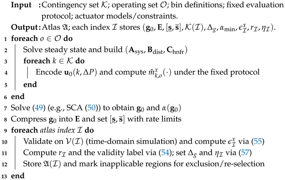
To make atlas generation reproducible, a recommended pipeline is as follows: (1) for each operating point o, solve the steady state and construct the explicit HNFR model $({\mathbf{A}}_{\mathrm{sys}},{\mathbf{B}}_{\mathrm{sys}},{\mathbf{C}}_{\mathrm{hnfr}})$ in Section 2 together with the disturbance input encoding; (2) under the fixed evaluation protocol, compute location sensitivity, surrogates, and (optionally) marginal benefit signals; (3) solve the robust allocation over $\mathcal{K}\times \mathcal{O}$ to obtain ${\mathbf{g}}_0$ and its feasibility/stability margins; (4) compress ${\mathbf{g}}_0$ into a structured executable form (e.g., zone sharing or clustering), thereby defining the low-dimensional scaling space; and (5) validate surrogate prediction against time domain simulations of the HNFR model (and, when available, higher-fidelity models), quantify conservative error bounds, and label inapplicable regions where linearization errors are amplified (e.g., ill-conditioned ${\mathbf{J}}_{LL}$, proximity to PLL instability boundaries, or strong current limiting). In addition to metric errors, we explicitly track the validity of the electromechanical-band approximation (13) within each atlas entry. For the same validation set $\mathcal{V}\left(\mathcal{I}\right)$ and RoCoF window $[0,T_{\mathrm{roc}}]$, define the normalized residual ratio

$$r_{\mathcal{I}}\triangleq \underset{(k,o)\in \mathcal{V}\left(\mathcal{I}\right)}{sup}\underset{t\in [0,T_{\mathrm{roc}}]}{sup}{\displaystyle \frac{\parallel {\mathit{\epsilon }}_{\dot{\mathit{\delta }},L}\left(t\right){\parallel }_{\infty }}{\parallel {\mathbf{K}}_{\mathrm{couple}}\mathsf{\Delta }{\mathit{\omega }}_S\left(t\right){\parallel }_{\infty }+{\mathit{\epsilon }}_0}},{\mathit{\epsilon }}_0>0,$$

(54)

where ${\mathit{\epsilon }}_{\dot{\mathit{\delta }},L}\left(t\right)$ is defined in (14) and ${\mathit{\epsilon }}_0$ prevents division by zero. Entries with $r_{\mathcal{I}}$ above a user-specified threshold (default 0.2) are labeled as “approximation-weak” and are assigned a smaller trust region ${\mathsf{\Delta }}_g$ together with increased margins ${\mathit{\delta }}_{\mathcal{I}}^x$ in (55) to retain conservativeness.

We compute conservative surrogate error bounds per entry and per metric. For $x\in \{\mathrm{roc},\mathrm{nad},\mathrm{spl}\}$, let $\mathcal{V}\left(\mathcal{I}\right)\subseteq \mathcal{K}\left(\mathcal{I}\right)\times \mathcal{O}$ be the validation scenario subset for index $\mathcal{I}$. Define

$${ϵ}_{\mathcal{I}}^x\triangleq \underset{(k,o)\in \mathcal{V}\left(\mathcal{I}\right)}{sup}{\left(m_{k,o}^x\left({\mathbf{g}}_0\right)-{\widehat{m}}_{k,o}^x\left({\mathbf{g}}_0\right)\right)}_{+}+{\mathit{\delta }}_{\mathcal{I}}^x,$$

(55)

where ${(·)}_{+}\triangleq max\{·,0\}$ and ${\mathit{\delta }}_{\mathcal{I}}^x\ge 0$ is a user-chosen margin to cover finite sampling and discretization in ${\mathcal{T}}_{\mathrm{roc}}$ and $\mathcal{T}$. These bounds support conservative screening by ensuring $m_{k,o}^x\left(\mathbf{g}\right)\le {\widehat{m}}_{k,o}^x\left(\mathbf{g}\right)+{ϵ}_{\mathcal{I}}^x$ for all $(k,o)\in \mathcal{K}\left(\mathcal{I}\right)\times \left\{o\right\}$ covered by the recorded validation protocol and for all $\mathbf{g}$ within the stored trust region. Hence, ${ϵ}_{\mathcal{I}}^x$ is jointly valid over the explicit location set $\mathcal{K}\left(\mathcal{I}\right)$, not only for the anchor index k appearing in (53). Reproducible margin decomposition. We set ${\delta }_{\mathcal{I}}^x\triangleq {\delta }_{\mathcal{I}}^{x,\mathrm{grid}}+{\delta }_{\mathcal{I}}^{x,\mathrm{sm}}+{\delta }_{\mathcal{I}}^{x,\mathrm{add}}$, where ${\delta }_{\mathcal{I}}^{x,\mathrm{grid}}$ is the time-grid discretization margin (Section 3), ${\delta }_{\mathcal{I}}^{x,\mathrm{sm}}$ bounds any smooth-envelope gap used inside SCA (Section 3), and ${\delta }_{\mathcal{I}}^{x,\mathrm{add}}$ is an optional extra conservativeness margin informed by RMS/DAE validation (e.g., bounded nonlinearities, quantization, or delay). Each component is stored in $\mathfrak{A}\left(\mathcal{I}\right)$ together with the protocol parameters. To avoid extrapolation beyond validation coverage, the bound ${ϵ}_{\mathcal{I}}^x$ is enforced only for $\mathbf{g}$ within the atlas-recorded trust region $\parallel \mathbf{g}-{\mathbf{g}}_0{\parallel }_{\infty }\le {\mathsf{\Delta }}_g$. In addition, ${\delta }_{\mathcal{I}}^x$ is selected per entry based on validation statistics to cover (i) sampling-set discretization and (ii) residual model mismatch, e.g., by combining a high-quantile of the observed positive error ${\left(m^x-{\widehat{m}}^x\right)}_{+}$ on $\mathcal{V}\left(\mathcal{I}\right)$ with an extra margin that accounts for the time grid resolution of ${\mathcal{T}}_{\mathrm{roc}}$ and $\mathcal{T}$. To make explicit this extension from ${\mathbf{g}}_0$ to the full trust region, ${\mathit{\delta }}_{\mathcal{I}}^{x,\mathrm{add}}$ is chosen so as to dominate the observed local drift of the positive surrogate error on a representative validation set $\mathcal{N}\left(\mathcal{I}\right)\subset \{\mathbf{g}:\parallel \mathbf{g}-{\mathbf{g}}_0{\parallel }_{\infty }\le {\mathsf{\Delta }}_g\}$, i.e.,

$${\delta }_{\mathcal{I}}^{x,\mathrm{add}}\ge \underset{\mathbf{g}\in \mathcal{N}\left(\mathcal{I}\right)}{sup}{\left[{\left(m^x\left(\mathbf{g}\right)-{\widehat{m}}^x\left(\mathbf{g}\right)\right)}_{+}-{\left(m^x\left({\mathbf{g}}_0\right)-{\widehat{m}}^x\left({\mathbf{g}}_0\right)\right)}_{+}\right]}_{+},$$

(56)

such that the stored bound remains locally conservative throughout the validated neighborhood. If this drift term is not small, then the entry is re-validated with a smaller ${\mathsf{\Delta }}_g$ and/or a larger ${\delta }_{\mathcal{I}}^{x,\mathrm{add}}$. Atlas parameters for deployment tightening. For each entry, we also record an estimated headroom-estimation relative error bound ${\epsilon }_{\mathcal{I}}^P,{\epsilon }_{\mathcal{I}}^E\in [0,1)$ (from measurement/estimation validation) and an entry-hit confidence $p_{\mathcal{I}}^{\mathrm{hit}}\in [0,1]$. The latter is defined as a conservative lower confidence bound on the probability that the online localization/bin-classification rule selects an atlas entry with an offline validation set matching the true regime. A conservative default tightening factor for use in deployment can be set as

$${\eta }_{\mathcal{I}}\triangleq \left(1-max\{{\epsilon }_{\mathcal{I}}^P,{\epsilon }_{\mathcal{I}}^E\}\right)·p_{\mathcal{I}}^{\mathrm{hit}},$$

(57)

which can be further reduced when the entry is labeled “approximation-weak” (large $r_{\mathcal{I}}$) or when the surrogate error bounds ${ϵ}_{\mathcal{I}}^x$ are large. Therefore, lower confidence, larger headroom uncertainty, or weaker local validation all decrease ${\eta }_{\mathcal{I}}$ monotonically and can only shrink the admissible set. Interpretation of ${\eta }_{\mathcal{I}}$: ${\eta }_{\mathcal{I}}$ is used to tighten the admissible set $\mathcal{G}\left(\widehat{\mathit{\rho }}\right)$ by shrinking $({\widehat{P}}_{max},{\widehat{E}}_{max})\mapsto (\eta {\widehat{P}}_{max},\eta {\widehat{E}}_{max})$ in (39) and (40); hence, decreasing $\eta$ is monotone-conservative with respect to feasibility under headroom uncertainty.

The full offline procedure is summarized in Algorithm 1.

Algorithm 1: Atlas Construction and Validation

4.2. Execution of Atlas-Based Scheduling

In execution, a set of scheduled gains is selected from the atlas and applied to the designated frequency support actuators. The same fixed measurement and evaluation protocol used in atlas construction is used to compute RoCoF/nadir/split metrics for reporting in Section 5. At each online update, the scheduler receives the current operating condition estimate $\widehat{\mathit{\rho }}$ and available headroom estimates. When a real-time localization module is available, it can additionally supply a disturbance location candidate set $\widehat{\mathcal{K}}$ with confidence scores and, when the event size is not known exactly, a disturbance magnitude estimate or interval $[\underline{\mathsf{\Delta }P},\overline{\mathsf{\Delta }P}]$; these inputs are treated as optional refinements that tighten the atlas selection rather than as prerequisites. In the baseline mode without online localization, $\widehat{\mathcal{K}}$ defaults to the full training set $\mathcal{K}$ of the matched atlas entry, meaning that the stored gains remain robust against all covered disturbance locations. Here, the logic is two-stage: $\widehat{\mathcal{K}}$ lives in the disturbance location space, while the candidate atlas entry set is obtained by lifting each $k\in \widehat{\mathcal{K}}$ to all atlas indices $\mathcal{I}=(k,o,\text{SCR-bin},\text{IBR-penetration-bin},\text{availability-bin})$ consistent with the observed bins and $\widehat{\mathit{\rho }}$. Denoting this lifted set by $\widehat{\mathfrak{I}}$, the scheduler retains only entries for which the lower bound of the hit confidence satisfies $p_{\mathcal{I}}^{\mathrm{hit}}\ge p_{min}$, the stored location coverage satisfies $\widehat{\mathcal{K}}\subseteq \mathcal{K}\left(\mathcal{I}\right)$, and the validated disturbance magnitude range contains the online estimate (or supports the corresponding conservative endpoint envelope), where $p_{min}\in (0,1)$ is a user-chosen acceptance threshold. Disturbance magnitude uncertainty does not create a separate entry index; instead, for every retained $\mathcal{I}$, the online verification is interpreted conservatively over the validated magnitude range associated with that entry, which is implemented by checking the relevant endpoint(s) when no monotonicity certificate is available. If several entries remain, the scheduler verifies them conservatively over the full recorded location set $\mathcal{K}\left(\mathcal{I}\right)$ together with the retained disturbance magnitude range, then accepts a single deployment entry ${\mathcal{I}}^{★}\in \widehat{\mathfrak{I}}$ with the smallest predicted worst-case normalized risk over $\mathcal{K}\left(\mathcal{I}\right)$. For the accepted entry ${\mathcal{I}}^{★}$, the online adjustment is restricted to the low-dimensional scaling $\mathbf{s}$ in (36). A lightweight execution problem is

$$\begin{array}{cc}\hfill \underset{\mathbf{s},\tau }{min}& \tau \hfill \\ \hfill \mathrm{s}.\mathrm{t}.& {\displaystyle \frac{{\widehat{m}}_{k,o}^{\mathrm{roc}}\left(\mathbf{g}\left(\mathbf{s}\right)\right)+{ϵ}_{{\mathcal{I}}^{★}}^{\mathrm{roc}}}{{\overline{m}}^{\mathrm{roc}}}}\le \tau ,\forall k\in \mathcal{K}\left({\mathcal{I}}^{★}\right),\hfill \\ \hfill & {\displaystyle \frac{{\widehat{m}}_{k,o}^{\mathrm{nad}}\left(\mathbf{g}\left(\mathbf{s}\right)\right)+{ϵ}_{{\mathcal{I}}^{★}}^{\mathrm{nad}}}{{\overline{m}}^{\mathrm{nad}}}}\le \tau ,\forall k\in \mathcal{K}\left({\mathcal{I}}^{★}\right),\hfill \\ \hfill & {\displaystyle \frac{{\widehat{m}}_{k,o}^{\mathrm{spl}}\left(\mathbf{g}\left(\mathbf{s}\right)\right)+{ϵ}_{{\mathcal{I}}^{★}}^{\mathrm{spl}}}{{\overline{m}}^{\mathrm{spl}}}}\le \tau ,\forall k\in \mathcal{K}\left({\mathcal{I}}^{★}\right),\tau \le 1,\hfill \\ \hfill & \mathbf{g}\left(\mathbf{s}\right)\in {\mathcal{G}}_{{\eta }_{{\mathcal{I}}^{★}}}\left(\widehat{\mathit{\rho }}\right),\mathbf{s}\in [{\underline{\mathbf{s}}}_{{\mathcal{I}}^{★}},{\overline{\mathbf{s}}}_{{\mathcal{I}}^{★}}],{\parallel \mathbf{g}\left(\mathbf{s}\right)-{\mathbf{g}}_{0,{\mathcal{I}}^{★}}\parallel }_{\infty }\le {\mathsf{\Delta }}_{g,{\mathcal{I}}^{★}},\hfill \\ \hfill & \alpha \left(\mathbf{g}\left(\mathbf{s}\right)\right)\le -{\alpha }_{min,{\mathcal{I}}^{★}},\hfill \end{array}$$

(58)

where ${\mathcal{G}}_{{\eta }_{{\mathcal{I}}^{★}}}\left(\widehat{\mathit{\rho }}\right)$ denotes the admissible set obtained from (39) and (40) after shrinking the headroom bounds by ${\eta }_{{\mathcal{I}}^{★}}$ and the remaining per-entry quantities in (58) are taken from $\mathfrak{A}\left({\mathcal{I}}^{★}\right)$. In particular, the accepted entry carries an explicit validated location set $\mathcal{K}\left({\mathcal{I}}^{★}\right)$, and the use of ${ϵ}_{{\mathcal{I}}^{★}}^x$ in (58) is justified jointly over that set rather than only at the anchor location embedded in the index. Because $dim\left(\mathbf{s}\right)\ll n_g$, (58) is intended as a low-dimensional lookup-and-verify step rather than as a full re-optimization of Section 3. When $\mathsf{\Delta }P$ is uncertain, the same admissibility, metric, and stability checks are interpreted against the validated disturbance magnitude range attached to ${\mathcal{I}}^{★}$, using endpoint evaluation unless a tighter monotonicity certificate has been recorded offline. After the candidate-set envelope check has selected ${\mathcal{I}}^{★}$, the acceptance sequence is intentionally strict: (1) check bin consistency, $p_{{\mathcal{I}}^{★}}^{\mathrm{hit}}$, and the coverage condition $\widehat{\mathcal{K}}\subseteq \mathcal{K}\left({\mathcal{I}}^{★}\right)$; (2) confirm that the online disturbance magnitude estimate lies inside the validated range of ${\mathcal{I}}^{★}$ (or else use its conservative endpoint envelope); (3) solve or clip $\mathbf{s}$ inside $[{\underline{\mathbf{s}}}_{{\mathcal{I}}^{★}},{\overline{\mathbf{s}}}_{{\mathcal{I}}^{★}}]$; (4) verify the trust region condition $\parallel \mathbf{g}-{\mathbf{g}}_{0,{\mathcal{I}}^{★}}{\parallel }_{\infty }\le {\mathsf{\Delta }}_{g,{\mathcal{I}}^{★}}$; (5) verify the metric bounds through ${\widehat{m}}^x+{ϵ}_{{\mathcal{I}}^{★}}^x$ over all $k\in \mathcal{K}\left({\mathcal{I}}^{★}\right)$; and (6) verify stability through (52). If any step fails, the scheduler first retries with a smaller $\eta$ or a more conservative candidate entry. If feasibility or stability is still not recovered or if all candidate entries have low confidence, the policy falls back to a location-agnostic pre-certified safe gain vector ${\mathbf{g}}_{\mathrm{safe}}^{\mathrm{glob}}(o,\mathrm{bins})$ stored offline with the atlas (or a companion safe table) and validated against all $k\in \mathcal{K}$ under the same protocol and over the same disturbance magnitude range. This fallback closes the online loop when localization is uncertain and prevents trust region claims from being used outside their validated domain.

An important practical consequence of the min–max formulation in (49) is that the online stage does not require explicit real-time identification of the disturbance bus. Because each atlas entry is optimized over the full candidate location set $\mathcal{K}\left(\mathcal{I}\right)$, the stored gain vector is already robust to any disturbance within that set for the indexed operating condition. Therefore, online execution selects the atlas entry by matching only the prevailing operating condition key. If real-time disturbance localization becomes available, it can serve as an optional refinement to narrow the conservativeness of the min–max hedge rather than as a prerequisite.

Regarding computational cost, the HNFR assembly scales as $O(n_S^3+n_L^3)$ for the network elimination step, which is dominated by the sparse solver with ${\mathbf{J}}_{LL}$. Although atlas construction involves repeated matrix-exponential evaluations, the per-entry cost remains tractable because the affine gain parameterization and low-dimensional scaling structure limit the number of required trajectory re-evaluations. For the IEEE 39-bus system, the full offline atlas construction completes within one minute on a standard workstation; by comparison, the online lookup and gain projection are instantaneous, requiring only a key-matching step and a bounded scaling operation. Communication requirements are limited to dispatching a small number of scalar gain setpoints to the GFM support buses at each dispatch update, which is compatible with existing supervisory control infrastructure operating on 5–15 min refresh cycles.

5. Case Studies

This section validates the framework developed in Section 2, Section 3 and Section 4 through three coordinated case studies: sensitivity to disturbance location, comparative coordination performance, and atlas-based online scheduling.

5.1. Test System

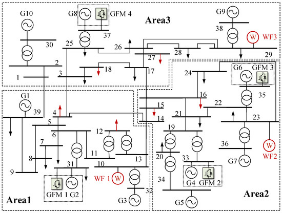
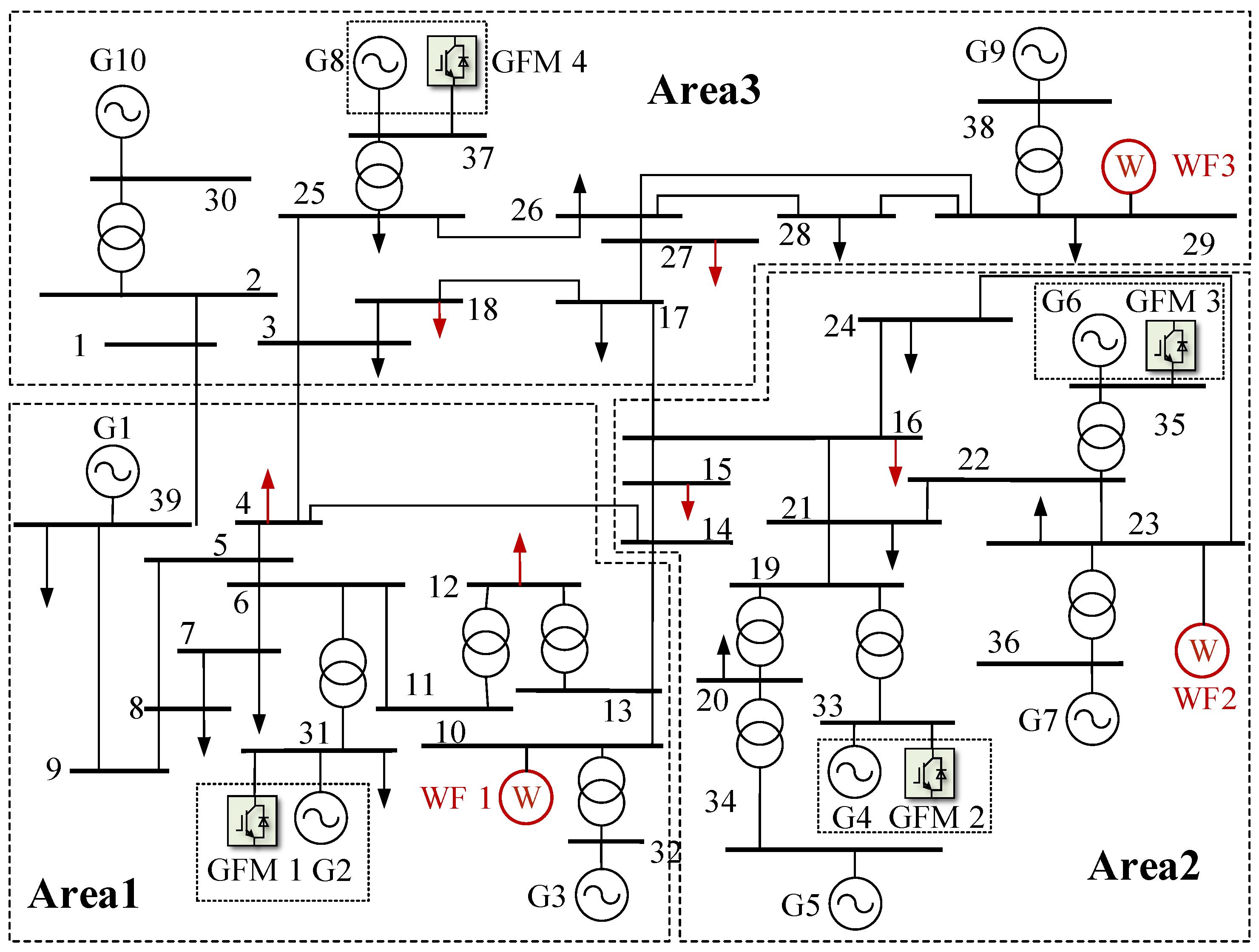
All studies are carried out on the modified IEEE 39-bus system shown in Figure 3. Relative to the benchmark network, three wind farms (WF1–WF3) are placed at Buses 10, 23, and 29 as GFL converter stations with PLL-based synchronization, with four tunable GFM-support buses (31, 33, 35, and 37) serving as the decision-variable locations for the $(H_i,D_i)$ allocation. In Figure 3, circles labeled WF1–WF3 denote the wind-farm GFL stations, GFM-icon buses 31, 33, 35, and 37 denote the tunable grid-forming support locations, red arrows denote the candidate disturbance buses (4, 12, 15, 16, 18, and 27), and solid black lines denote transmission corridors. The network is further partitioned into three areas following the conventional New England boundary, as indicated by the dashed zones in Figure 3. This partitioning groups the ten support buses (30–39) by electrical proximity, and is used later in the area-wise comparison in Section 5 to interpret how the optimized allocations redistribute inertia and damping across the system. The comparative studies then reuse the same three parameter files, namely, the Original setting, the HNFR-optimized setting, and the COI-optimized setting, meaning that the reported differences reflect coordination logic rather than inconsistent data preparation.

Figure 3. Structure of the modified IEEE 39-bus system.

Two disturbance families are used. First, all waveform comparisons are locked to a single prescribed event, namely, a 250 MW active power increase at load Bus 4 injected at $t=2.0$ s. Second, the location sensitivity and atlas-audit studies sweep the disturbance location over Buses 4, 12, 15, 16, 18, and 27 under the same disturbance magnitude. In every case, the compared methods share the same support portfolio, the same $0.005$ s simulation grid, and the same RoCoF/nadir/split definitions, providing a common basis for interpreting nodal and aggregated responses.

Table 1 fixes the common protocol used by all case study comparisons in this section. Table 2 then reports the three GFM-side parameter configurations used throughout the case studies, namely, the Original setting taken from the baseline model, the HNFR-optimized setting obtained from the proposed location-aware tuning, and the COI-optimized setting obtained from the aggregated-frequency benchmark. Consistent with Section 3, the listed $H/D$ values are effective coefficients mapped from the writable GFM frequency support setpoints in (32) and (33). Therefore, the differences among the three columns represent different closed-loop support allocations across Buses 31, 33, 35, and 37 rather than changes to all internal converter-control parameters in the Section 2 device model.

Table 1. Compact case study protocol.

Item	Setting
Network	Modified IEEE 39-bus test system; wind farms WF1/WF2/WF3 at Buses 10, 23, and 29; tunable support buses at 31, 33, 35, and 37.
Fixed waveform case	Bus 4, 250 MW step at $t=2.0$ s on a $0.005$ s simulation grid; used for waveform and budget-matched comparisons.
Location sweep	Disturbance buses 4, 12, 15, 16, 18, and 27 under the same disturbance magnitude.

Table 2. GFM-side $H/D$ settings.

Bus	Original		HNFR		COI
	$\mathit{H}$	$\mathit{D}$	$\mathit{H}$	$\mathit{D}$	$\mathit{H}$	$\mathit{D}$
31	4.329	2.800	5.115	5.366	3.463	2.926
33	3.575	6.500	3.719	2.600	5.248	9.750
35	4.350	7.600	3.877	18.079	6.525	11.400
37	3.471	3.400	7.732	1.360	5.207	2.720

5.2. Disturbance Location Sensitivity and Heterogeneous Nodal Responses

The six disturbance buses (4, 12, 15, 16, 18, and 27) used in this subsection constitute the candidate location set $\mathcal{K}$ over which the atlas in Section 4 is constructed. Therefore, the following waveform and metric comparisons simultaneously serve as cross-scenario evidence and atlas training set diagnostics.

The first study characterizes how disturbance location reshapes heterogeneous nodal frequency behavior under a common disturbance magnitude and common support portfolio. A fixed Bus 4 event is used for waveform inspection, then the disturbance location is swept over six buses for metric comparison. The resulting evidence quantifies whether worst-node RoCoF, nadir, and nodal split are governed primarily by a system-average response or by spatially localized stress patterns that require explicit disturbance location modeling.

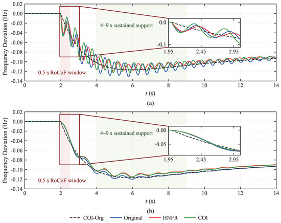
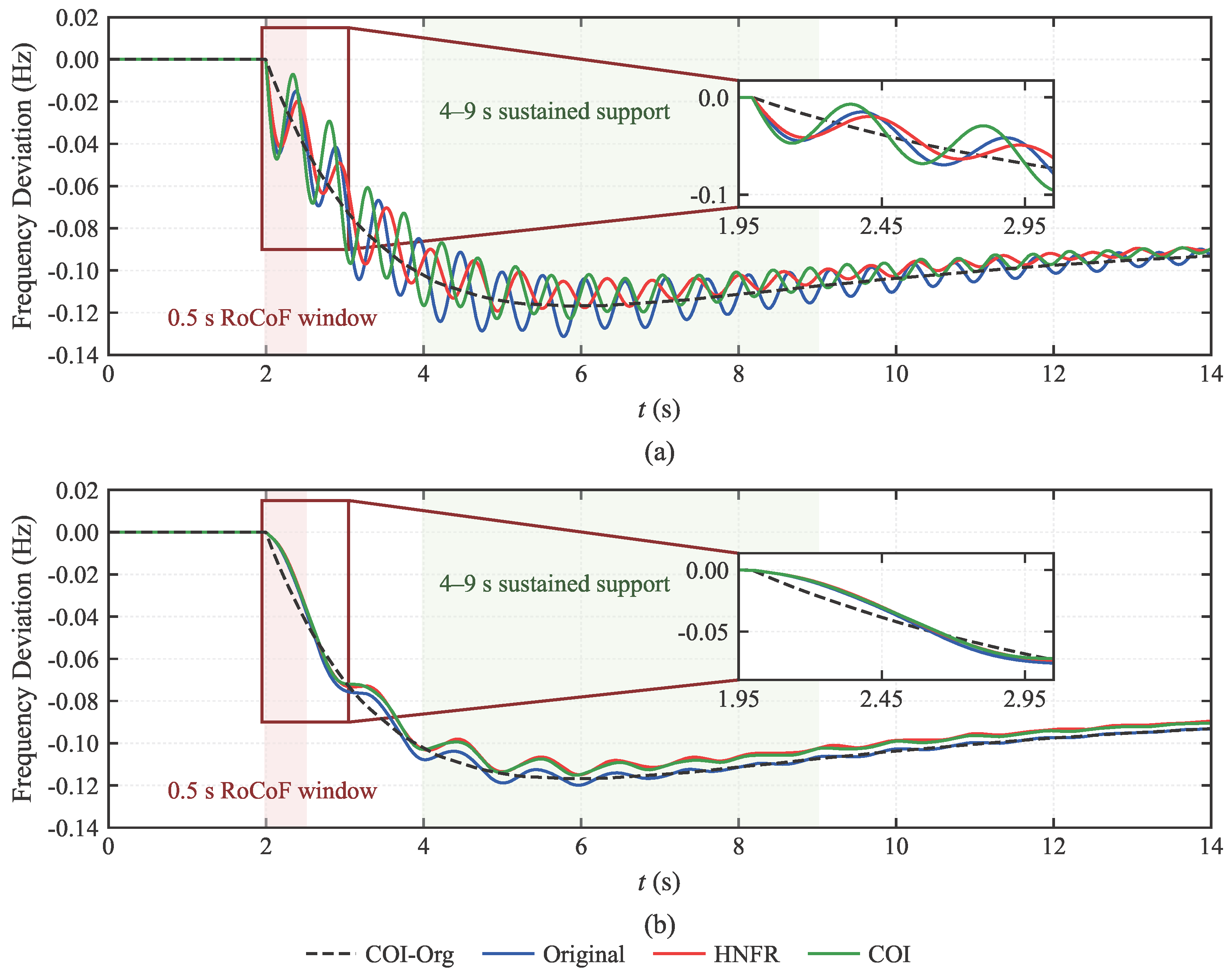
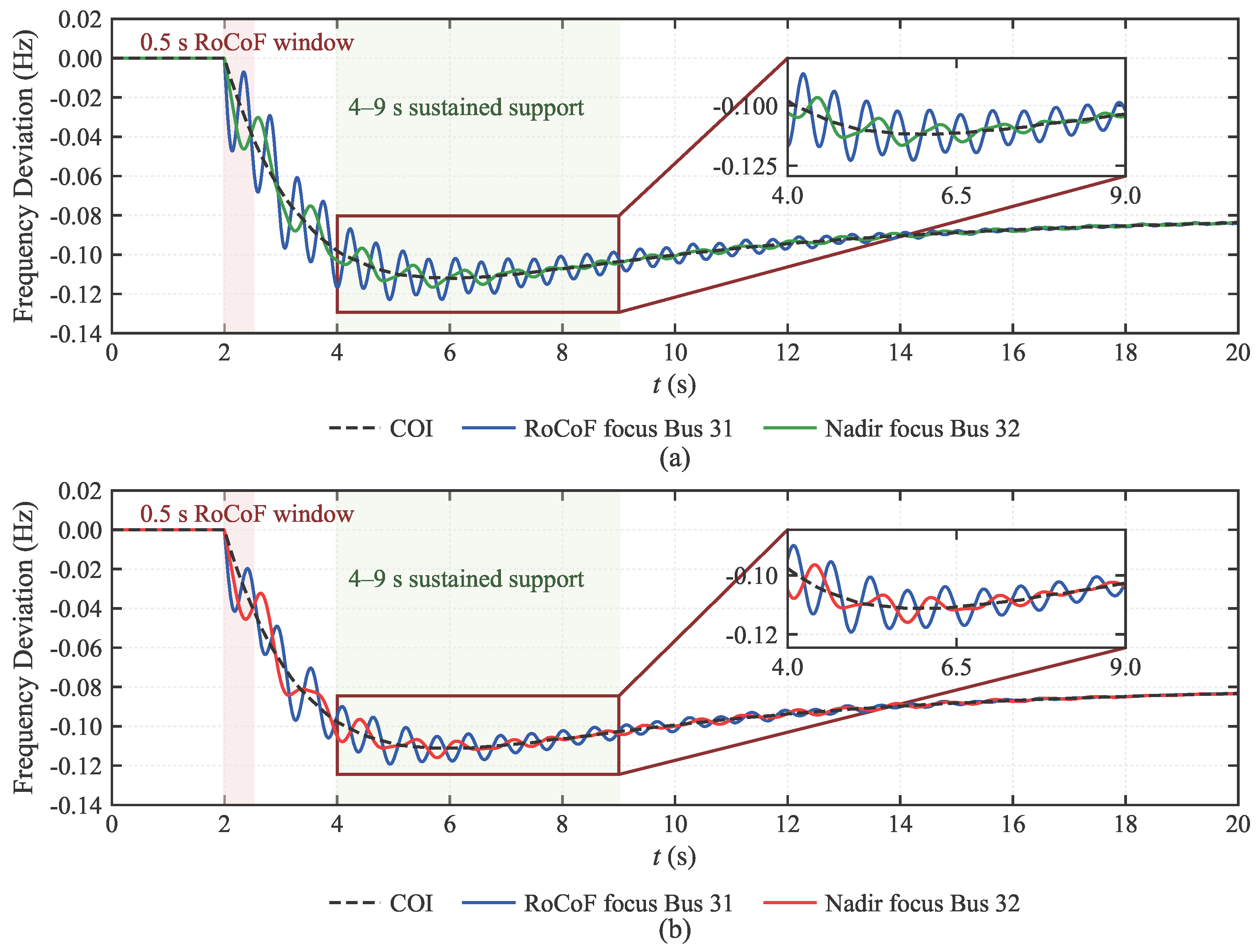
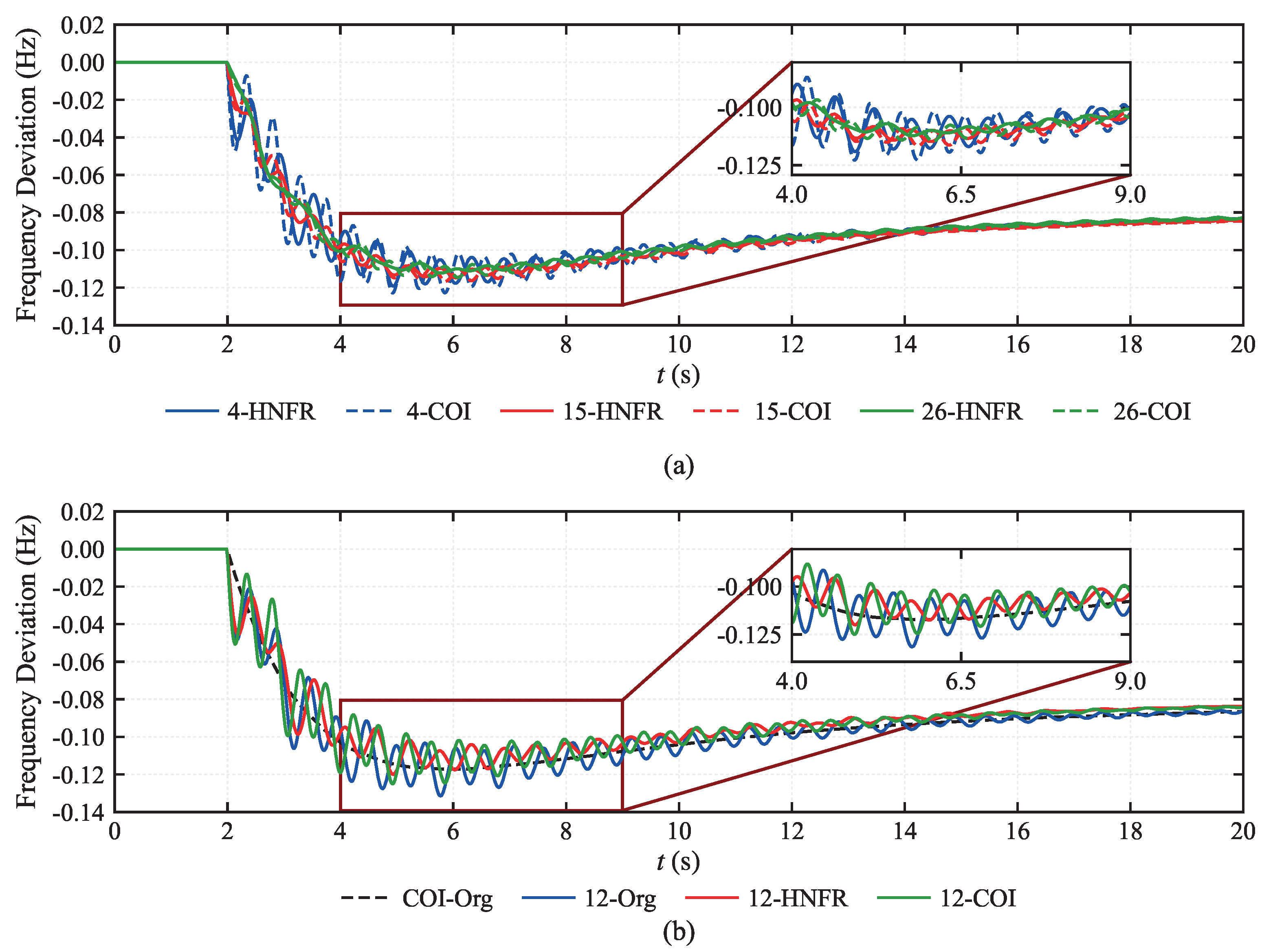
The trajectory comparison in Figure 4 shows that the early transient was much more pronounced at the stressed GFM-side Bus 31 than at the remote synchronous-machine Bus 38. Figure 4a shows that at Bus 31, the Original, HNFR, and COI responses separated clearly during the first few seconds after the event; the inset confirms that the largest inter-method deviation was concentrated in the early post-disturbance window rather than in the late quasi-steady segment. Figure 4b shows that the Bus 38 traces remained comparatively smooth and stayed closer to the COI reference. This two-panel comparison identifies a localized transient burden that is only weakly reflected by the aggregated COI trajectory.

Figure 4. (a) Representative trajectories at the stressed GFM-side Bus 31 under the fixed Bus 4, 250 MW disturbance; (b) representative trajectories at the remote SG Bus 38 under the same disturbance.

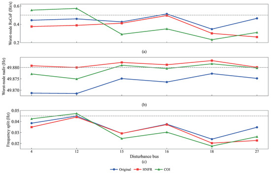
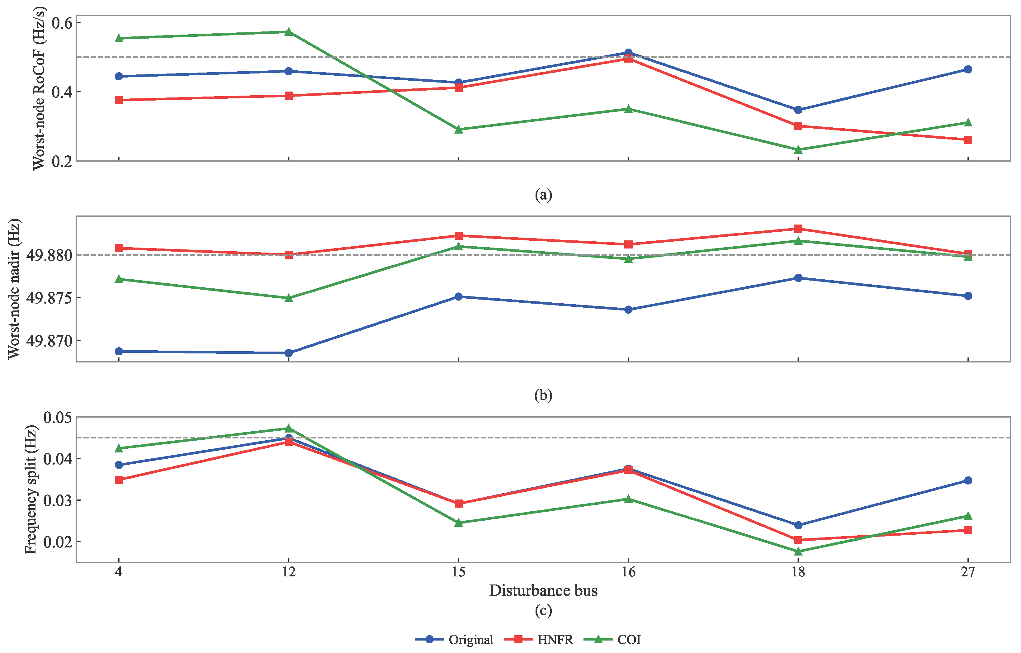
Figure 5 compares the Original, HNFR, and COI parameter sets over the same six-bus disturbance sweep under a unified simulation chain. Figure 5a shows that the worst-node RoCoF burden remained strongly location dependent and was not minimized by the same method at every disturbance bus: the most adverse RoCoF occurred at Bus 16 for the Original and HNFR settings, but shifted to Bus 12 for the COI setting. Figure 5b,c shows an even clearer concentration pattern. For all three parameter sets, Bus 12 produced both the deepest worst-node nadir and the largest maximum nodal frequency split; thus, the dominant stress concentration remained tied to a specific disturbance location instead of being distributed uniformly over the network.

Figure 5. (a) Location sweep of worst-node RoCoF over the six candidate disturbance buses, (b) location sweep of worst-node nadir over the same disturbance set, and (c) location sweep of the maximum nodal frequency split. The horizontal dashed lines indicate the corresponding design/security thresholds used as references for comparison across the three parameter settings.

Across the three curves, the HNFR setting consistently reduces the most restrictive nadir and split outcomes relative to the COI tuning, limiting the minimum nadir to 49.8800 Hz and the maximum split to 0.0440 Hz, whereas the corresponding COI results are 49.8749 Hz and 0.0473 Hz. The advantage of RoCoF remains more scenario-dependent, but the overall ranking in Figure 5 shows a smaller nodal risk envelope under the location-aware heterogeneous formulation than under the aggregated tuning objective.

The location-dependent patterns in Figure 5 can be traced analytically to the initial RoCoF relation in (27): for a unit disturbance at bus k, the initial RoCoF at each observation node is determined by ${\left[{\mathbf{C}}_{\mathrm{hnfr}}{\mathbf{B}}_{\mathrm{sys}}\right]}_{i,k}$, which encodes the electrical coupling between the disturbance bus and each observation bus through the network admittance and effective inertia distribution. Within the test system, the dominant factor is the electrical distance to the nearest GFM-support unit: Buses 4 and 12 produce the most severe worst-node responses because they are electrically remote from the support cluster at Buses 33, 35, and 37 and are primarily served by Bus 31 alone.

For practical context, the observed worst-node RoCoF values across all six disturbance locations remain below 0.56 Hz/s, and the worst-node nadir deviation remains within 0.13 Hz of nominal. These values are well within standard RoCoF relay thresholds (typically 0.5–1.0 Hz/s) and first-stage under-frequency load shedding levels (typically 49.0–49.2 Hz). The security constraints used in the min–max allocation are design-level specifications set tighter than the protection thresholds, meaning that the inter-method gap between HNFR and COI in Figure 5 reflects differences in margin utilization rather than proximity to system protection limits.

5.3. Comparative Performance of Location-Aware Coordination

The second study compares the Original, HNFR, and COI parameter settings under the same fixed disturbance, simulation grid, and response-processing pipeline. The comparison is carried out under a matched total GFM support budget, meaning that differences among the three methods are attributable to allocation strategy rather than support quantity. Waveform traces at the dominant stressed buses and event-level security metrics are evaluated jointly under the same event.

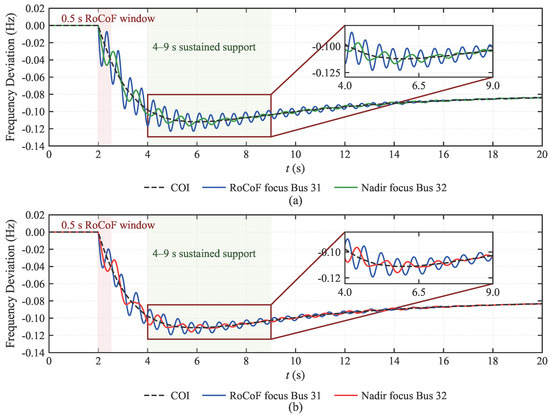
Under the budget-matched comparison in Figure 6, the dominant nodal stress remained concentrated around Bus 31, whereas the aggregated COI trajectory changed much less across methods. Figure 6a shows that the COI-tuned case preserved the system-average response but left a deeper dip at the stressed node and a larger separation between the local and aggregated trajectories. Figure 6b shows that the HNFR-tuned case reduced the depth of the stressed-node excursion and tightened the separation between the nodal and COI traces while maintaining a comparable aggregate response. Therefore, under the same total support budget, the HNFR setting corresponds to a stronger redistribution of support toward the electrically stressed location and a smaller local security burden than the COI-oriented allocation.

Figure 6. (a) Budget-matched COI response under the fixed Bus 4, 250 MW disturbance and (b) budget-matched HNFR response under the same disturbance.

Table 3 quantifies the fixed-disturbance comparison among the three parameter sets. Relative to the Original setting, HNFR reduced the worst-node RoCoF by 15.43%, improved the worst-node nadir by 0.0121 Hz, and reduced the maximum frequency split by 9.25%. Relative to the COI setting, HNFR further reduced the worst-node RoCoF by 32.20%, improved the worst-node nadir by 0.0036 Hz, and reduced the maximum split by 17.78%, while the COI nadir changed only marginally. The largest performance separation appears in the nodal-security metrics, whereas the aggregated COI nadir remains comparatively close across the tuned cases.

Table 3. Comparison of the three parameter sets under the fixed Bus 4 250 MW disturbance.

Method	Worst-Node RoCoF (Hz/s)	Worst-Node Nadir (Hz)	Max Frequency Split (Hz)	COI Nadir (Hz)
Original	0.4442	49.8687	0.0385	49.8832
HNFR	0.3757	49.8808	0.0349	49.8888
COI	0.5541	49.8771	0.0424	49.8879

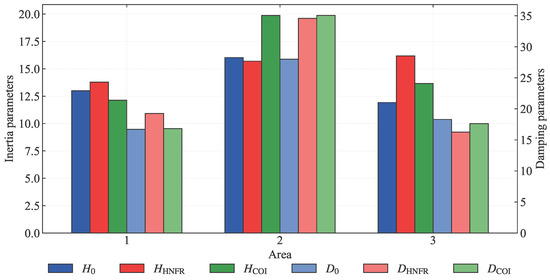
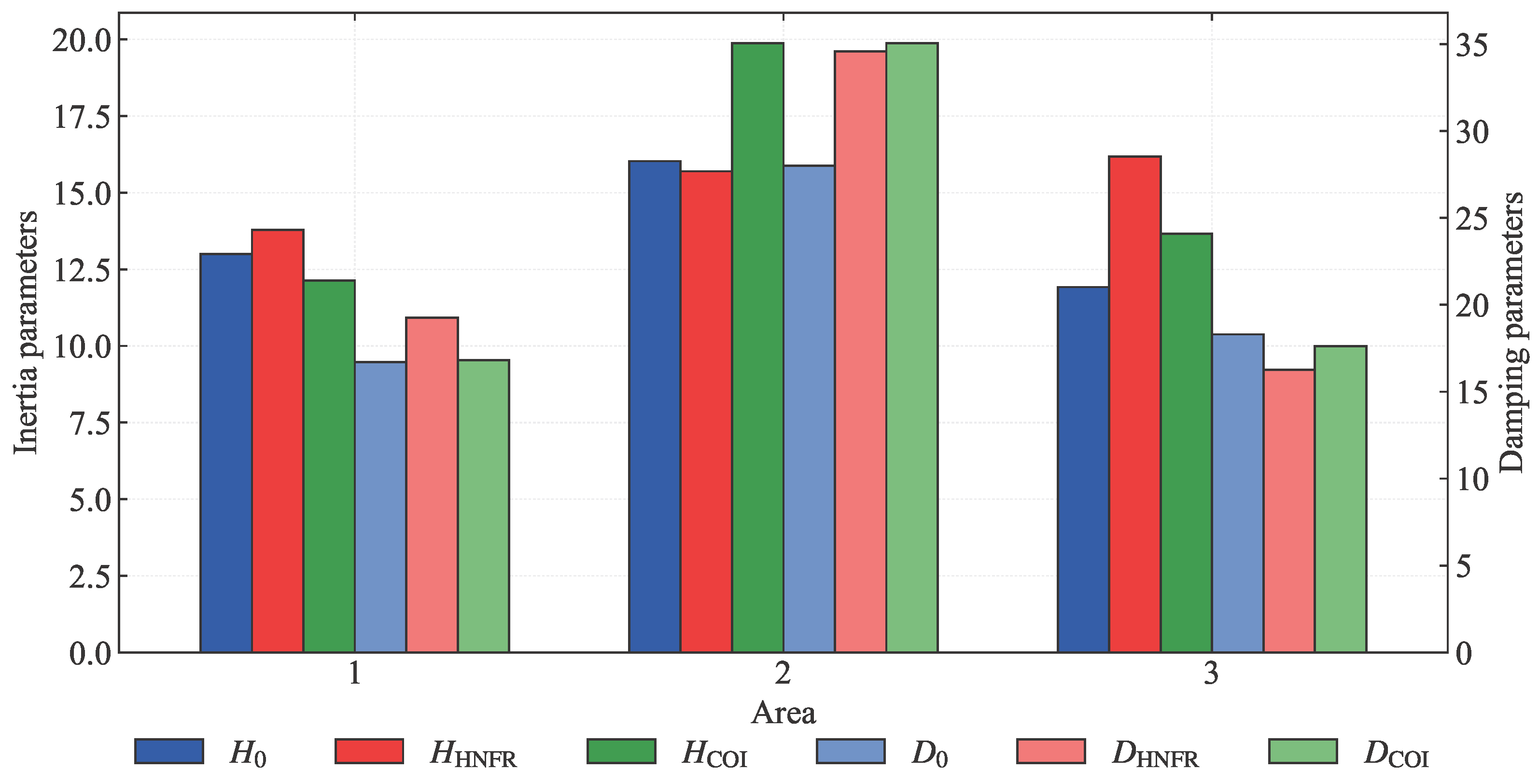
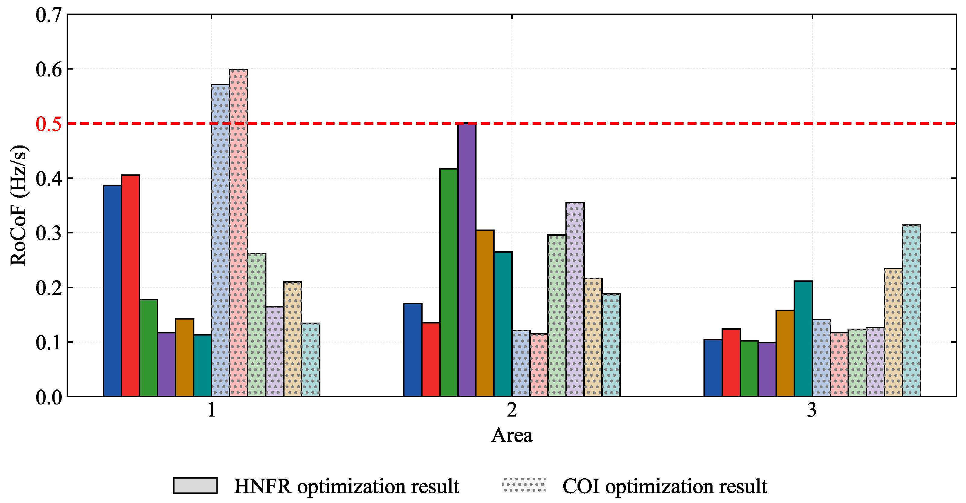
Figure 7 shows how the three parameter sets redistribute effective inertia and droop across the three areas. The inertia bars indicate that the HNFR and COI solutions allocate inertia differently from the Original setting and from each other, with the HNFR solution shifting more effective support toward the electrically stressed area rather than preserving the baseline distribution. The damping bars show the same non-uniform trend for the droop, where the HNFR-tuned configuration concentrates damping support more selectively than the COI benchmark. These area-wise allocation changes are consistent with the smaller stressed-node excursions observed in Figure 4 and Figure 6, and show that the HNFR improvement is achieved through spatial reallocation rather than through uniform increase of all GFM support parameters.

Figure 7. Area-wise comparison of effective inertia and droop allocation under the Original, HNFR, and COI parameter settings.

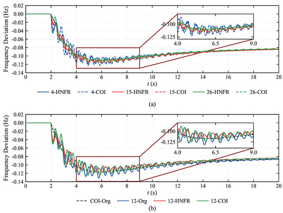
Across the broader set of representative scenarios in Figure 8, the aggregated COI trajectories remain relatively close, but the nodal trajectories separate more visibly during the initial dip and in the recovery-stage inset. Therefore, the same pattern observed for the fixed Bus 4 disturbance is retained across multiple disturbance locations; inter-method differences remain modest in the aggregate trajectory, and become more pronounced in the stressed nodal responses.

Figure 8. (a) Representative nodal frequency response comparison across selected disturbance scenarios and (b) close-up comparison of the Original, HNFR, and COI responses under the most severe representative scenario.

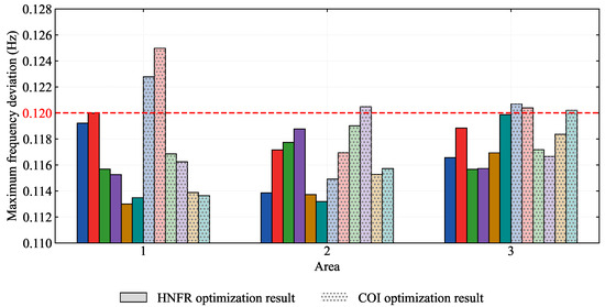
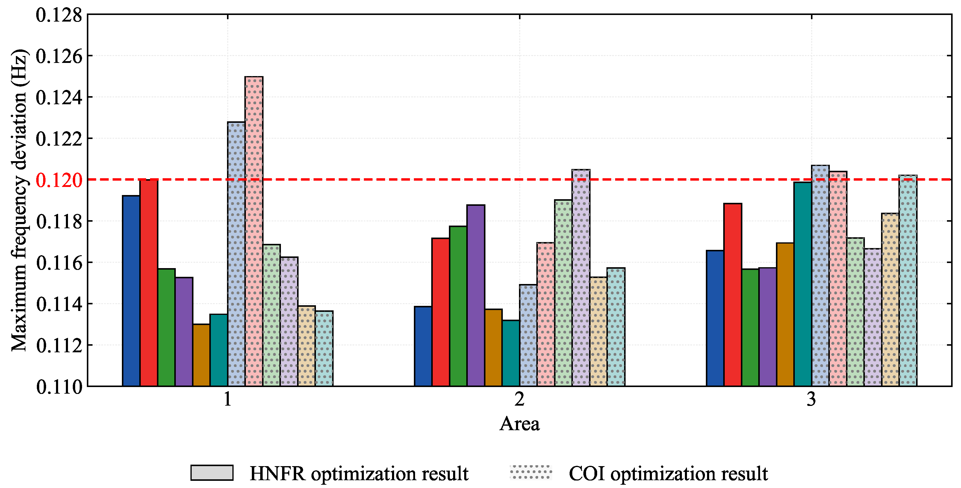
The nadir-oriented cross-scenario comparison in Figure 9 extends the comparison from a single event to the full six-bus disturbance set, focusing on the most restrictive frequency deviation outcome in each scenario. In Figure 9, the red dashed line denotes the design-level frequency-deviation threshold used as a security reference, and the paired bars at each disturbance location correspond to the HNFR and COI settings, respectively. Across all reported locations, the HNFR setting yielded smaller worst-node deviations than the COI setting, with the most severe case occurring at Bus 12 and being limited to 0.119989 Hz under HNFR versus 0.124978 Hz under COI. Therefore, the nadir ordering remains unchanged when the disturbance location is swept systematically.

Figure 9. Cross-scenario comparison of maximum frequency deviations under the HNFR and COI parameter settings.

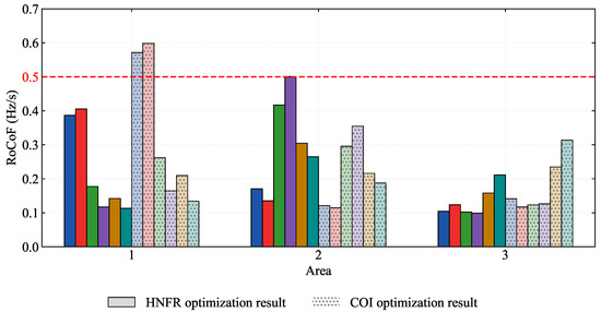
The RoCoF-oriented evidence in Figure 10 complements the nadir comparison by examining the fastest local transient over the same six disturbance locations. In Figure 10, the red dashed line denotes the design-level RoCoF threshold used as a security reference, and the paired bars at each disturbance location correspond to the HNFR and COI settings, respectively. Figure 10 shows that the RoCoF ranking is more scenario-dependent than the nadir ranking: HNFR reduces the worst-node RoCoF at Buses 4 and 12, whereas the COI setting remains slightly better at several other disturbance locations. For both methods, the spread across the curves remains strongly location-dependent. Among the cross-scenario results, the most consistent HNFR advantage appears in nadir and split, while the RoCoF benefit depends more strongly on the disturbance location and the spatial distribution of transient stress.

Figure 10. Cross-scenario comparison of worst-node RoCoF under the HNFR and COI parameter settings.

To assess the sensitivity of the scheduled gains to parameter uncertainty, the HNFR-optimized $(H,D)$ vector was perturbed by independent uniform random factors drawn from $[0.85,1.15]$ across all four GFM buses, then the worst-node metrics were re-evaluated over the same six disturbance locations for 20 random samples. The 95th-percentile worst-node nadir deviation remained within 1.6% of the baseline value and the 95th-percentile maximum split variation remained within 1.9%, indicating that the allocation is not sensitive to moderate gain uncertainty in the reported operating regime.

Taken together, the case studies show strong dependence on disturbance location, clear separation among heterogeneous nodal frequency channels, and systematic benefits from worst-node-oriented coordination in low-inertia systems. Aggregated COI behavior alone does not reveal the most restrictive transient risk, whereas the HNFR-based formulation provides stronger stressed-node security than the Original and COI parameter settings across the reported waveform and metric comparisons.

6. Discussion

This paper develops a disturbance location-aware frequency support framework for low-inertia systems with heterogeneous frequency channels. The proposed HNFR model preserves the distinction among SG/GFM electromechanical frequencies and GFL PLL-estimated frequencies, enabling reproducible evaluation of worst-node RoCoF, nadir, and nodal frequency split under location-specific disturbances. The main implication of the reported results is that frequency security in low-inertia systems with heterogeneous converter channels is governed by nodal stress concentration rather than by a single aggregate indicator. Across the waveform comparisons, disturbance location sweep, and budget-matched tuning study, the most restrictive transient burden remains concentrated at a small set of buses and is not represented faithfully by the COI trajectory alone. By preserving the separation among SG electromechanical frequencies, GFM-controlled responses, and GFL PLL-estimated frequencies, the HNFR formulation resolves the nodal stress patterns that determine whether support allocation is protective at those buses that experience the most severe transients.

The case studies also delimit the present engineering scope of the method. The HNFR setting improves stressed-node nadir and reduces nodal split more consistently than the competing settings, whereas the RoCoF comparison remains scenario-dependent, indicating that different transient objectives continue to impose competing design pressures. Extending the method toward faster online scheduling would require further progress in model refinement, uncertainty handling, and implementation-level acceleration.

The HNFR model is derived under the quasi-stationary voltage assumption and electromechanical-scale linearization around a given operating point. These assumptions exclude large-signal voltage dynamics, converter current-limiting behavior, and nonlinear saturation effects that may become significant under severe disturbances. Within the moderate disturbance range used in the case studies (250 MW active-power step), the reported results remain internally consistent across the presented scenarios; broader validation against EMT-class or large-disturbance simulation is identified as future work.

Regarding parameter sensitivity, the min–max formulation provides an inherent hedge against worst-case disturbance locations within the candidate set. A full Monte Carlo sensitivity study covering parameter uncertainty, measurement noise, and communication delay is identified as future work. Extending the atlas to span additional scenario axes such as load level, renewable energy penetration, and network topology would further strengthen the robustness characterization, and is a natural next step for larger-scale deployments.

References

- Gu, Y.; Green, T.C. Power System Stability with a High Penetration of Inverter-Based Resources. Proc. IEEE 2023, 111, 832–853. [Google Scholar] [CrossRef] [Scilit]
- Yan, K.; Li, G.; Zhang, R.; Xu, Y.; Jiang, T.; Li, X. Frequency Control and Optimal Operation of Low-Inertia Power Systems with HVDC and Renewable Energy: A Review. IEEE Trans. Power Syst. 2024, 39, 4279–4295. [Google Scholar] [CrossRef] [Scilit]
- Al Kez, D.; Foley, A.M.; Ahmed, F.; Morrow, D.J. Overview of frequency control techniques in power systems with high inverter-based resources: Challenges and mitigation measures. IET Smart Grid 2023, 6, 447–469. [Google Scholar] [CrossRef] [Scilit]
- Khan, M.; Wu, W.; Li, L. Grid-forming control for inverter-based resources in power systems: A review on its operation, system stability, and prospective. IET Renew. Power Gener. 2024, 18, 887–907. [Google Scholar] [CrossRef] [Scilit]
- Sajadi, A.; Rañola, J.A.; Kenyon, R.W.; Hodge, B.M.; Mather, B. Dynamics and Stability of Power Systems with High Shares of Grid-Following Inverter-Based Resources: A Tutorial. IEEE Access 2023, 11, 29591–29613. [Google Scholar] [CrossRef] [Scilit]
- Tan, B.; Zhao, J.; Netto, M.; Krishnan, V.; Terzija, V.; Zhang, Y. Power system inertia estimation: Review of methods and the impacts of converter-interfaced generations. Int. J. Electr. Power Energy Syst. 2022, 134, 107362. [Google Scholar] [CrossRef] [Scilit]
- Chen, X.; Jiang, Y.; Terzija, V.; Lu, C. Review on measurement-based frequency dynamics monitoring and analyzing in renewable energy dominated power systems. Int. J. Electr. Power Energy Syst. 2024, 155, 109520. [Google Scholar] [CrossRef] [Scilit]
- Deng, X.; Mo, R.; Wang, P.; Chen, J.; Nan, D.; Liu, M. Review of RoCoF Estimation Techniques for Low-Inertia Power Systems. Energies 2023, 16, 3708. [Google Scholar] [CrossRef] [Scilit]
- Yin, H.; Wu, Y.; Qiu, W.; Zeng, C.; You, S.; Tan, J.; Hoke, A.; Kruse, C.J.; Rockwell, B.W.; Kawamura, K.A.; et al. Precise ROCOF estimation algorithm for low inertia power grids. Electr. Power Syst. Res. 2022, 209, 107968. [Google Scholar] [CrossRef] [Scilit]
- Azizi, S.; Sun, M.; Liu, G.; Terzija, V. Local Frequency-Based Estimation of the Rate of Change of Frequency of the Center of Inertia. IEEE Trans. Power Syst. 2020, 35, 4948–4951. [Google Scholar] [CrossRef] [Scilit]
- Wang, T.; Ma, S.; Wang, S.; Hou, W.; Gao, J.; Guo, J.; Zhou, X. Modal Analysis-Based Analytical Method for Frequency Estimation During Inertia Response Stage of Power Systems. IEEE J. Emerg. Sel. Top. Circuits Syst. 2023, 13, 692–701. [Google Scholar] [CrossRef] [Scilit]
- Wang, L.; Ren, J.; Huang, G.; Xie, L.; Feng, C.; Zhang, Y. Identifying the Largest RoCoF and Its Implications. IEEE Trans. Power Syst. 2025, 40, 1164–1167. [Google Scholar] [CrossRef] [Scilit]
- Wang, J.; Zhang, J.; Hou, Q.; Jiang, H.; Strbac, G.; Teng, F.; Zhang, N. Analytical Decomposition of Nodal Frequency Responses. IEEE Trans. Power Syst. 2025, 40, 1176–1179. [Google Scholar] [CrossRef] [Scilit]
- Badesa, L.; Teng, F.; Strbac, G. Conditions for Regional Frequency Stability in Power System Scheduling—Part I: Theory. IEEE Trans. Power Syst. 2021, 36, 5558–5566. [Google Scholar] [CrossRef] [Scilit]
- Kerci, T.; Milano, F. Asymmetry of Frequency Distribution in Power Systems: Sources, Estimation, Impact and Control. IEEE Open Access J. Power Energy 2025, 12, 135–145. [Google Scholar] [CrossRef] [Scilit]
- Wang, X.; Li, W.; Shen, J.; Ding, Q. Reduced-Order Bus Frequency Response Model for Bulk Power Systems. J. Mod. Power Syst. Clean Energy 2025, 13, 1127–1138. [Google Scholar] [CrossRef] [Scilit]
- Milano, F.; Ortega, A. Frequency Divider. IEEE Trans. Power Syst. 2016, 32, 1493–1501. [Google Scholar] [CrossRef] [Scilit]
- Gao, H.; Xin, H.; Huang, L.; Li, Z.; Huang, W.; Wu, C.; Ju, P. Common-Mode Frequency in Converter-Integrated Power Systems: Definition, Analysis, and Quantitative Evaluation. IEEE Trans. Power Syst. 2022, 37, 4846–4860. [Google Scholar] [CrossRef] [Scilit]
- Li, J.; Li, Y.; Li, W.; Yang, S.; Du, Z. System Power Imbalance Estimation Utilizing Linear Component of Local Frequency. IEEE Trans. Power Syst. 2024, 39, 2373–2376. [Google Scholar] [CrossRef] [Scilit]
- Liu, J.; Wang, C.; Bi, T. Revisiting the Effect of Grid-Following Converter on Frequency Dynamics - Part I: Center of Inertia. IEEE Trans. Power Syst. 2026, 41, 1441–1458. [Google Scholar] [CrossRef] [Scilit]
- Liu, J.; Wang, C.; Bi, T. Revisiting the Effect of Grid-Following Converter on Frequency Dynamics - Part II: Spatial Difference. IEEE Trans. Power Syst. 2026, 41, 1459–1472. [Google Scholar] [CrossRef] [Scilit]
- Trujillo, M.; Sajadi, A.; Shaw, J.; Hodge, B.M. Analytical Models of Frequency and Voltage in Large-Scale All-Inverter Power Systems. IEEE Trans. Power Syst. 2026, 1–12. [Google Scholar] [CrossRef] [Scilit]
- Ducoin, E.A.S.; Gu, Y.; Chaudhuri, B.; Green, T.C. Analytical Design of Contributions of Grid-Forming and Grid-Following Inverters to Frequency Stability. IEEE Trans. Power Syst. 2024, 39, 6345–6358. [Google Scholar] [CrossRef] [Scilit]
- Askarian, A.; Park, J.; Salapaka, S. Enhanced Grid-Following (E-GFL) Inverter: A Unified Control Framework for Stiff and Weak Grids. IEEE Trans. Power Electron. 2024, 39, 5089–5107. [Google Scholar] [CrossRef] [Scilit]
- Zhou, W.; Mohammed, N.; Bahrani, B. Comprehensive Modeling, Analysis, and Comparison of State-Space and Admittance Models of PLL-Based Grid-Following Inverters Considering Different Outer Control Modes. IEEE Access 2022, 10, 30109–30146. [Google Scholar] [CrossRef] [Scilit]
- Carreño, M.; Velasco-Falguera, O.; Arévalo-Soler, J.; Gomis-Bellmunt, O. RMS+: Augmenting the Traditional Circuit Model to Capture PLL Instability. IEEE Trans. Power Deliv. 2026, 41, 364–374. [Google Scholar] [CrossRef] [Scilit]
- Shang, L.; Hua, Z.; Liu, C.; Dong, X.; Jiao, F.; Li, Y. Modelling and analysis of grid frequency dynamics with equivalent inertia characteristic of grid-forming voltage source converters. CSEE J. Power Energy Syst. 2024, 1–13. [Google Scholar] [CrossRef]
- Wang, Z.; Shan, Y.; Zhu, Y.; Liu, R.; Gu, Y. Spatio-Temporal Frequency Distribution Analysis in Systems with Grid-Forming and Grid-Following Inverters: A New Perspective From Frequency Domain. IEEE Access 2025, 13, 87999–88011. [Google Scholar] [CrossRef] [Scilit]
- Liyanage, C.; Meegahapola, L.; Nutkani, I.; Jalili, M. Strategic Placement of Grid-Forming Inverters Considering Spatiotemporal Dynamics and Composite Stability Index. IEEE Open J. Ind. Electron. Soc. 2025, 6, 290–308. [Google Scholar] [CrossRef] [Scilit]
- Ni, F.; Nijhuis, M.; Nguyen, P.H.; Cobben, J.F.G. Variance-Based Global Sensitivity Analysis for Power Systems. IEEE Trans. Power Syst. 2018, 33, 1670–1682. [Google Scholar] [CrossRef] [Scilit]
- Poolla, B.K.; Bolognani, S.; Dorfler, F. Optimal Placement of Virtual Inertia in Power Grids. IEEE Trans. Autom. Control 2017, 62, 6209–6220. [Google Scholar] [CrossRef] [Scilit]
- Poolla, B.K.; Gross, D.; Dorfler, F. Placement and Implementation of Grid-Forming and Grid-Following Virtual Inertia and Fast Frequency Response. IEEE Trans. Power Syst. 2019, 34, 3035–3046. [Google Scholar] [CrossRef] [Scilit]
- Golpira, H.; Atarodi, A.; Amini, S.; Messina, A.R.; Francois, B.; Bevrani, H. Optimal Energy Storage System-Based Virtual Inertia Placement: A Frequency Stability Point of View. IEEE Trans. Power Syst. 2020, 35, 4824–4835. [Google Scholar] [CrossRef] [Scilit]
- Zhao, T.; Parisio, A.; Milanovic, J.V. Location-dependent distributed control of battery energy storage systems for fast frequency response. Int. J. Electr. Power Energy Syst. 2021, 125, 106493. [Google Scholar] [CrossRef] [Scilit]
- Han, R.; Hu, Q.; Zhang, H.; Ge, Y.; Quan, X.; Wu, Z. Robust allocation of distributed energy storage systems considering locational frequency security. Int. J. Electr. Power Energy Syst. 2024, 157, 109903. [Google Scholar] [CrossRef] [Scilit]
- Liu, D.; Yang, Q.; Chen, Y.; Chen, X.; Wen, J. Optimal Parameters and Placement of Hybrid Energy Storage Systems for Frequency Stability Improvement. Prot. Control Mod. Power Syst. 2025, 10, 40–53. [Google Scholar] [CrossRef] [Scilit]
- Ekomwenrenren, E.; Tang, Z.; Simpson-Porco, J.W.; Farantatos, E.; Patel, M.; Hooshyar, H. Hierarchical Coordinated Fast Frequency Control Using Inverter-Based Resources. IEEE Trans. Power Syst. 2021, 36, 4992–5005. [Google Scholar] [CrossRef] [Scilit]
- Zhao, X.; Xue, Y.; Zhang, X.P. Fast Frequency Support From Wind Turbine Systems by Arresting Frequency Nadir Close to Settling Frequency. IEEE Open Access J. Power Energy 2020, 7, 191–202. [Google Scholar] [CrossRef] [Scilit]
- Lyu, X.; Gross, D. Grid Forming Fast Frequency Response for PMSG-Based Wind Turbines. IEEE Trans. Sustain. Energy 2024, 15, 23–38. [Google Scholar] [CrossRef] [Scilit]
- Lavi, Y.; Apt, J. Inverter fast frequency response is a low-cost alternative to system inertia. Electr. Power Syst. Res. 2023, 221, 109422. [Google Scholar] [CrossRef] [Scilit]
- Peng, Z.; Peng, Q.; Zhang, Y.; Han, H.; Yin, Y.; Liu, T. Online Inertia Allocation for Grid-Connected Renewable Energy Systems Based on Generic ASF Model With Frequency Nadir Constraint. IEEE Trans. Power Syst. 2024, 39, 1615–1627. [Google Scholar] [CrossRef] [Scilit]
Disclaimer/Publisher’s Note: The statements, opinions and data contained in all publications are solely those of the individual author(s) and contributor(s) and not of MDPI and/or the editor(s). MDPI and/or the editor(s) disclaim responsibility for any injury to people or property resulting from any ideas, methods, instructions or products referred to in the content. |
© 2026 by the authors. Licensee MDPI, Basel, Switzerland. This article is an open access article distributed under the terms and conditions of the Creative Commons Attribution (CC BY) license.