Deep6DHead: A 6D Head Pose Estimation Method Based on Deep Feature Enhancement

Abstract

To address the bottlenecks of accuracy in head pose estimation caused by occlusion and rotational representation ambiguities, we propose Deep6DHead, a 6-degree-of-freedom (6DoF) head pose estimation method based on deep feature enhancement. This method innovatively integrates RGB and depth information to construct a four-channel input and achieves feature fusion of RGB-D through a dual-branch network. First, a Squeeze-and-Excitation (SE) module adaptively weights the depth geometric features of key anatomical regions to achieve channel recalibration. Second, based on the 6DoF rotation representation framework, we introduce an anatomical constraint loss using the nasal bridge normal. This constraint corrects rotation deviations caused by noise by enforcing consistency in local geometric orientation. Finally, the model outputs the rotation matrix end-to-end for final pose estimation. Experiments on the 300W-LP, BIWI, and AFLW2000 datasets demonstrate that our method significantly improves robustness and accuracy, particularly under extreme head poses. Notably, it achieves state-of-the-art performance on the roll axis (lowest error: 2.05) and a competitive overall MAE of 3.45, providing an effective solution for head pose estimation in complex real-world scenarios including extreme viewing angles.

1. Introduction

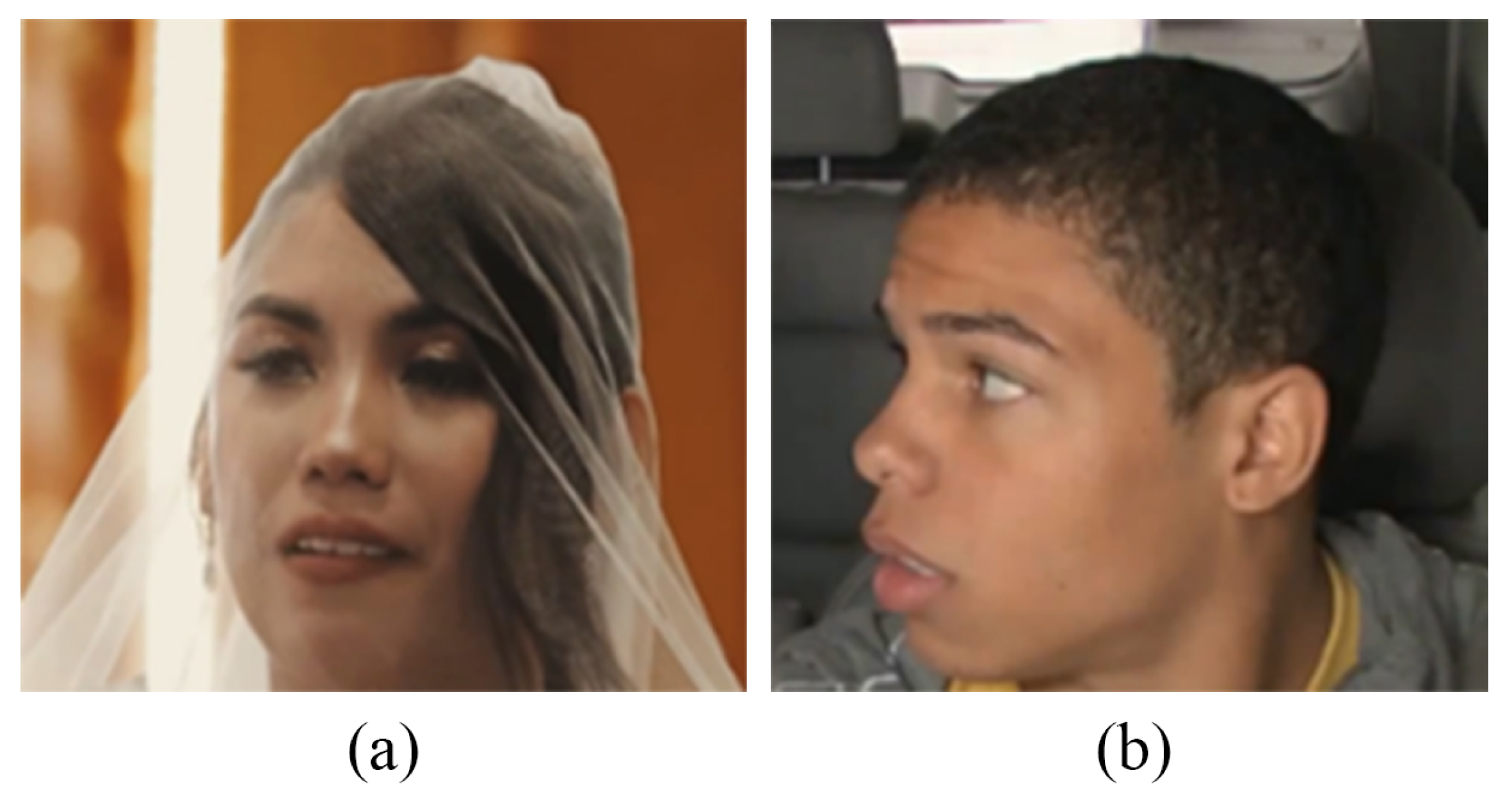
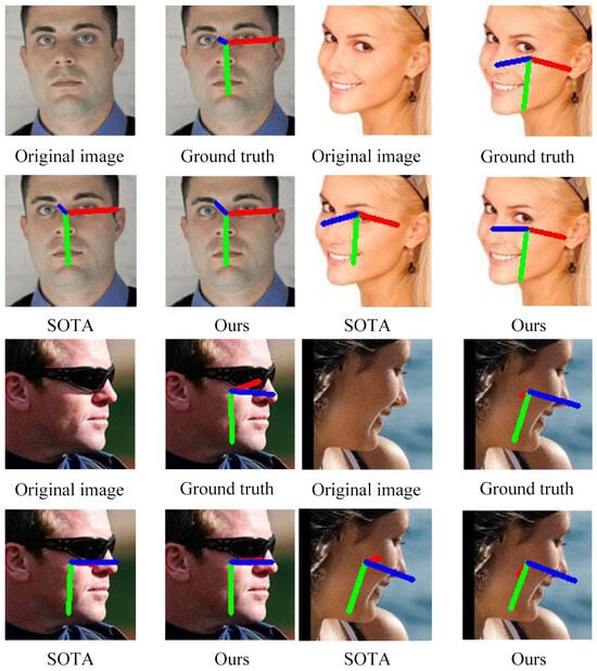
Accurate head pose estimation in 3D space is a fundamental task in computer vision, with widespread application value in fields such as cervical spine mobility measurement in medicine [1], driver fatigue detection [2], augmented reality interfaces [3], and natural human–computer interaction [4]. Methods for head pose estimation can be broadly categorized into two types: landmark-based [5,6,7] and landmark-free [8,9,10,11]. Landmark-based methods first detect precise facial key points. Then, they use geometric algorithms like Perspective-n-Point (PnP) [12] to estimate head pose, achieving high accuracy when key points are clearly visible. However, such methods face significant challenges in practical applications: facial occlusion and extreme head angles can easily lead to key point detection failure, as shown in Figure 1, thereby affecting both the reliability of the pipeline and the accuracy of the final pose estimate.

These difficulties connect to a wider pattern: key point pipelines inherit landmark fragility under occlusion and large viewpoints (Figure 1), monocular RGB limits 3D structure, pose outputs require stable parameterizations, and depth or pseudo-depth should agree with local surface geometry despite noise. Deep6DHead adopts a landmark-free regressor [8,9,10,11], builds on 6D rotation codes [13], and augments this framework with RGB–D fusion and an anatomy-aware normal loss; Section 2 contrasts the underlying learning paradigms in more detail.

Figure 1. Examples of challenging conditions in facial imagery, using representative RGB crops from the public benchmarks employed in this work (300W-LP [14], BIWI [15], and AFLW2000 [16]; dataset protocol in Section 4). (a) Facial occlusion: a crop in which a substantial part of the face is not visible in the image plane due to foreground occlusion (reduced visible facial area). (b) Extreme head pose: a crop in which the head is far from a frontal view (large absolute yaw).

Figure 1. Examples of challenging conditions in facial imagery, using representative RGB crops from the public benchmarks employed in this work (300W-LP [14], BIWI [15], and AFLW2000 [16]; dataset protocol in Section 4). (a) Facial occlusion: a crop in which a substantial part of the face is not visible in the image plane due to foreground occlusion (reduced visible facial area). (b) Extreme head pose: a crop in which the head is far from a frontal view (large absolute yaw).

To overcome these limitations, recent research has shifted focus toward landmark-free end-to-end methods [8,9,10,11]. These methods directly regress pose parameters from the input image, circumventing the dependency on intermediate landmark detection and thus effectively avoiding error accumulation caused by key point detection failures. Through end-to-end deep learning frameworks, the model learns the global mapping relationship from the raw image to pose parameters, often improving stability under landmark failure while optimizing average pose accuracy on benchmark splits. Current methods mostly use standard RGB images. However, these images struggle with self-occlusion. These limitations put a fundamental cap on how accurate the models can be in complex real-world scenes.

To break through the geometric perception limitations of the RGB modality, our work introduces depth information to form a four-channel RGB–D input. Depth maps encode surface relief and head shape cues that complement RGB appearance, partially compensating for the limited 3D structure available from monocular color images alone. Nevertheless, under the landmark-free end-to-end paradigm, how to efficiently fuse multi-modal information and accurately model the 3D rotation space still faces two core challenges.

The first challenge is the effective fusion of multi-modal features. Although depth data can provide stable geometric information, existing methods struggle to fully utilize its advantages. On one hand, there is a lack of strong correlation modeling between the geometric features of the depth channel and the rotation parameters; on the other hand, noise from depth sensors can be amplified during the orthogonalization process, causing the predicted rotation matrix to deviate from geometric rationality.

The second challenge is the accurate modeling of the rotation space. Traditional representations (such as Euler angles and quaternions) suffer from issues such as Gimbal lock or topological ambiguity [17]. Although 6DoF [13] codes can alleviate many of these shortcomings, they still face problems such as depth noise disrupting the orthogonality of the recovered rotation matrix and a lack of anatomical constraints, which reduces geometric plausibility in RGB-D settings.

The main contributions of this work are summarized as follows:

1.

Designing an end-to-end landmark-free dual-branch RGB–depth pipeline (with SE recalibration on both branches) for 6DoF head pose: although dual-branch RGB–D encoding, SE-style recalibration, and 6D rotation regression are standard in isolation, we orchestrate them with monocular depth estimation (MiDaS pseudo-depth) when native RGB-D benchmarks are unavailable and use SE to emphasize geometric features in key anatomical regions (e.g., the nasal bridge and eye sockets), unifying depth geometric and RGB appearance cues for landmark-free rotation regression.

2.

Proposing a depth-normal consistency loss that links depth gradients to the predicted rotation on $\mathrm{SO}\left(3\right)$, instantiating a reusable local normal–rotation consistency prior, the nasal bridge serves as the primary patch because of its structural stability and reliable depth gradients, yaw-adaptive gating adjusts constraint strength under extreme viewpoints, and the same template extends to other rigid depth-stable facial patches (Section 3.2).

3.

Reporting improved roll MAE and modest overall MAE gains versus the strong RGB-only baseline 6DRepNet [13] on BIWI and AFLW2000 under the standard protocol (Table 2), while other listed methods remain competitive on yaw and pitch; claims are scoped to the cited benchmarks.

The remainder of this paper is organized as follows. Section 2 reviews related work, including landmark-based approaches, a structured categorization of landmark-free learning paradigms (classification-based, regression-based, and rotation-representation-based families), and rotation uncertainty techniques. Section 3 presents our proposed Deep6DHead method, detailing the depth-attention fusion mechanism and the anatomically driven direction loss. Section 4 provides experimental results and ablation studies. Section 5 discusses limitations and outlook. Section 6 concludes.

2. Related Work

2.1. Landmark-Based Head Pose Estimation Methods

Landmark-based methods aim to predict head pose by detecting facial landmarks, solving the 2D and 3D correspondence problem. While they can achieve high accuracy when landmarks are reliable, performance heavily depends on the accuracy of facial landmarks and external head information. FAN [6] proposed a heatmap regression-based method to solve 2D and 3D face alignment. Baltrusaitis et al. [18] used an average human model and depth data to solve the correspondence between 2D facial landmarks and the 3D model. OsGG-Net [7] proposed a one-step graph generation network to estimate 3D pose angles, where the generated facial landmarks serve as nodes to construct a landmark connection graph.

Furthermore, some methods utilize multi-task learning to jointly model multiple facial attribute estimations. Hyper Face [19] proposed a CNN architecture that simultaneously performs face detection, landmark localization, head pose estimation, and gender recognition. MNN [20] proposed an encoder–decoder CNN architecture for head pose, facial landmark location, and visibility estimation, leveraging a large amount of in-the-wild landmark annotation data.

However, these landmark-based approaches exhibit inherent limitations. Their performance is fundamentally constrained by how accurate and reliable the initial facial landmark detection is, which is known to degrade significantly under challenging conditions. This is because the facial landmark annotations typically used for alignment, lacking regional anatomical reference, often contain pose-irrelevant information and frequently fail in scenes with large pose variations and partial occlusions [7,20].

2.2. Categorization of Landmark-Free Learning Paradigms

Beyond the landmark-based versus landmark-free split, recent landmark-free methods differ in how pose is encoded and optimized. Table 1 summarizes four widely used families—(i) classification and hybrid schemes that quantize pose and often refine within bins; (ii) direct regression on Euler angles or decoupled scalars; (iii) rotation-representation-based regression using quaternions, 6D continuous codes mapped to SO(3), or full rotation matrices with orthogonalization; and (iv) probabilistic or generative modeling on SO(3). This taxonomy clarifies where Deep6DHead sits: we follow the rotation-representation line [13,21,22] but additionally inject RGB–D geometry and an anatomical surface-normal consistency term, emphasizing 3D structure, stable rotation modeling, and depth–surface geometric alignment—goals largely orthogonal to the binning-versus-regression debate. The following subsection reviews representative networks in greater detail.

Table 1. Structured comparison of mainstream landmark-free head pose learning paradigms (illustrative examples; not exhaustive). Deep6DHead combines rotation-representation-based regression with RGB–D fusion and a depth-normal prior.

Paradigm	Typical Formulation	Examples	Common Limitations
Classification/ hybrid	Binned pose labels, often plus fine regression within bins	HopeNet [8]; wide-range binning (e.g., WHENet [23])	Quantization and bin design vs. fine resolution
Direct angle regression	${\ell }_2$/robust loss on Euler angles or factorized angles	FSA-Net [11]; FDN [9]	Gimbal lock, ambiguity [17,24]
Rotation-constrained rep.	Quat., 6D→SO(3), matrix + orthogonalization	QuatNet [21]; 6DRepNet [13]; img2pose [22]	Often RGB-only; weak explicit 3D geometric priors
Probabilistic/ diffusion on SO(3)	Distributional or generative rotation modeling	MFDNet [25]; HeadDiff [17]	Data, training complexity, compute
Deep6DHead (ours)	6D regression + dual-branch RGB–D + anatomical normal loss	This work	Requires depth or pseudo-depth (Section 4.2)

2.3. Landmark-Free Head Pose Estimation Methods

Table 1 supplies a structured map of learning paradigms; here we survey concrete architectures. Landmark-free methods directly learn facial features from a given image, modeling the relationship between the face image and head pose labels. Hope Net [8] proposed a multi-loss network that directly extracts Euler angles (yaw, pitch, and roll) from images through joint classification and regression. FSA-Net [11] introduced a coarse-to-fine regression and feature aggregation method that uses pixel-level spatial information of feature maps to predict Euler angles. FDN [9] maps discriminative features for each Euler angle to three corresponding latent variable subspaces. Quan Net [21] aimed to use quaternions instead of Euler angles and a sequential regression loss to avoid ambiguity in head pose. MFD Net [25] employed the matrix Fisher distribution to mitigate disturbances and ambiguities in standard head pose representations. Pan et al. [26] proposed a novel self-paced paradigm to enable deep discriminative models to improve head pose estimation performance. FASHE [10] uses a single frontal reference image to extract range blocks and transform them into good approximations of domain blocks in the target image. Image2pose [22] regresses the 6-degree-of-freedom (6DoF) facial pose to generate a bounding box for aligning 3D faces without landmarks and face detection. ASG [27] proposed an anisotropic spherical Gaussian label distribution to ensure the network learns adjacent head poses with an unbiased expectation. Token HPE [28] proposed a key-few relation-aware method that uses a Transformer architecture to learn multiple orientation labels for regions encoding direction and learns region similarity for facial orientation. Continuous rotation representations have been shown to help alleviate the ambiguity and discretization of head pose labels. However, these methods still face several limitations. Many approaches overlook the intrinsic uncertainty and discontinuity of rotation representations, which can lead to instability in angle regression. Moreover, because the inherent ambiguity in pose allows visually similar facial appearances to correspond to multiple plausible poses and this ambiguity is often not explicitly modeled, the method’s robustness decreases under real-world variations such as illumination, occlusion, and identity differences.

In recent years, significant progress has been made in 3D head pose estimation research. 3DMM-based methods model facial features by regressing 3D Morphable Model parameters and treat head pose estimation as an auxiliary task. 3DDFA [14] uses a CNN to fit a 3D face model to an RGB image, achieving accurate landmark alignment even under extreme poses and occlusion. Head Fusion [29] developed an adaptive framework that supports 360-degree head tracking and multi-angle pose estimation. 3DDFAv2 [30] adopted a meta-joint optimization strategy to regress 3DMM parameters, significantly improving performance. Synergy Net [31] proposed a two-stage synergistic network for precise 3D landmark prediction through point feature refinement. DAD-3DHeads [32] constructed a large-scale diversified dataset and developed a 3D mesh prediction method based on the FLAME model. Although these 3DMM methods achieve state-of-the-art results, they suffer from high dependency on large-scale 3D annotated data, which is costly and labor-intensive to acquire. This constraint often limits their generalization capability in unconstrained real-world scenarios, where facial appearance, expression, and environmental conditions vary widely. Furthermore, the performance of such methods can degrade significantly under large poses or severe occlusions due to their reliance on complete facial geometry.

To address these issues, we introduce depth information as a 3D supplement, fusing RGB-D data to reduce dependence on expensive 3D annotations and improve generalization in complex scenes.

2.4. Uncertainty in Rotation Regression

Recent research on rotation uncertainty estimation has focused on the choice of probability distribution and rotation representation. Prokudin et al. [33] proposed using a binomial network to predict the probability distribution parameters of Euler angles. Deng et al. [34] employed the Bingham distribution to model the 3D rotation of quaternion representations and their uncertainty. However, Zhou et al. [24] proved that any rotation representation in four or fewer dimensions is discontinuous and unsuitable for neural network learning tasks.

Therefore, researchers have turned to more robust SO(3) representations: Mohlin et al. [35] utilized the matrix Fisher distribution to learn the probability distribution of rotation matrices; Wu et al. [36] introduced a non-parametric implicit distribution on SO(3) for rotation regression of symmetric objects; Yin et al. [37] proposed a new family of probability distributions on SO(3), termed the rotation Laplace distribution; Wang et al. [17] employed an isotropic Gaussian distribution on SO(3) to model uncertainty; and Thorsten Hempel’s team [13] improved computational efficiency via a 6D rotation representation. Consequently, probabilistic modeling in SO(3) space has become a mainstream trend, and incorporating more discriminative geometric and anatomical information is the key to advancing this field toward practical application. Probabilistic SO(3) heads and deterministic 6D regression are complementary: distributions capture ambiguity and calibration, whereas 6D+Gram–Schmidt offers a lightweight point-estimate pipeline that couples cleanly with geodesic losses. We adopt the 6D parameterization of Hempel et al. [13] as the rotation head and allocate novelty to depth fusion and anatomical–geometric regularization rather than to replacing probabilistic models wholesale. To address this, our method introduces depth information and a nasal bridge normal loss to enhance the perception of facial anatomical structures, thereby improving the discrimination and accuracy of rotation estimation.

3. Method

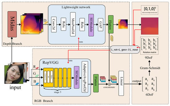
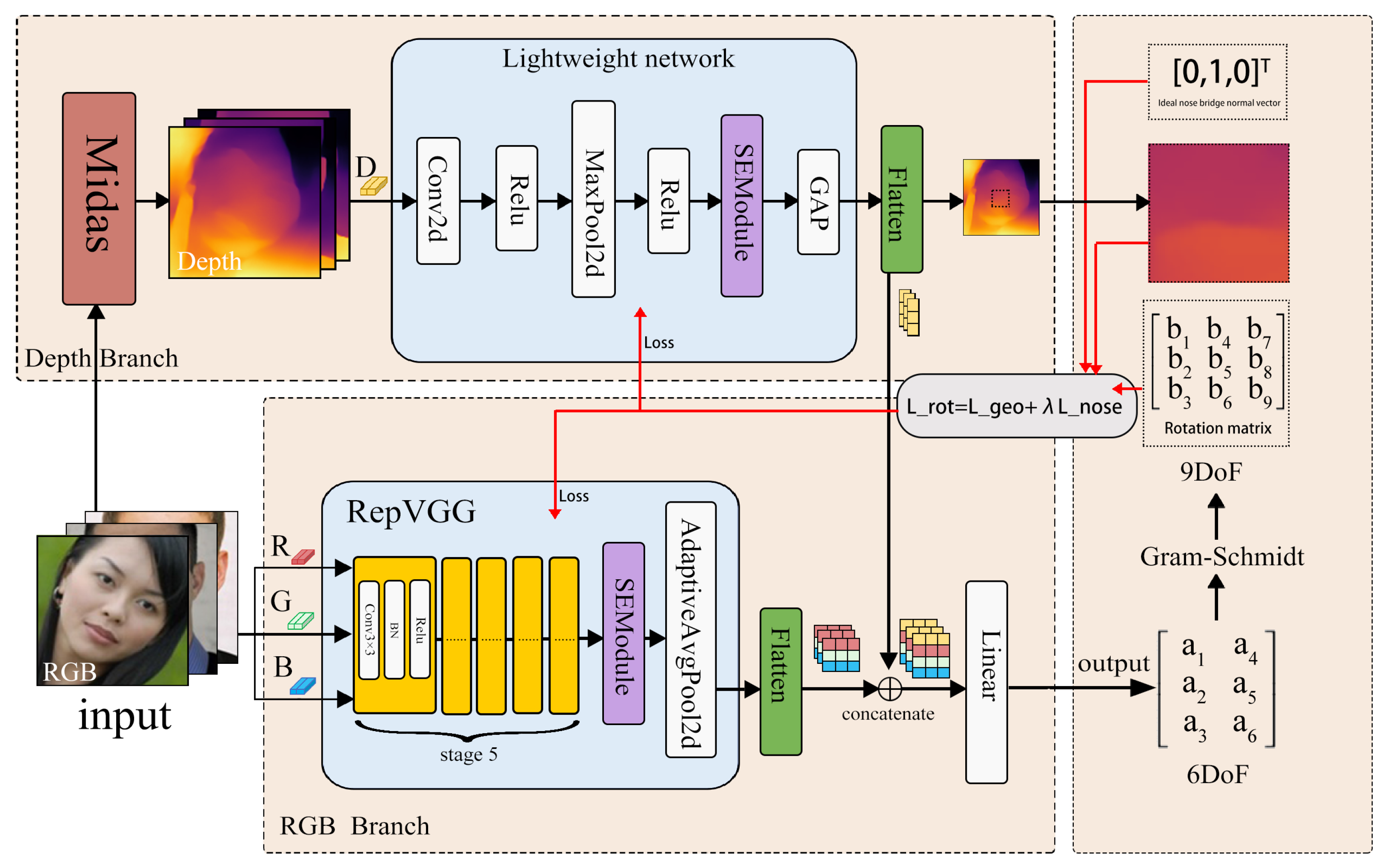
This research is based on the 6D rotation representation by Thorsten Hempel et al. [13] and proposes a head pose estimation method that integrates depth perception and anatomical constraints. Following common practice in the recent head pose literature, we adopt continuous 6D rotation codes and Gram–Schmidt orthogonalization [13]; our methodological emphasis is on depth-guided feature fusion and the anatomical normal regularizer rather than on redesigning the rotation head itself. As shown in Figure 2, our network architecture adopts a dual-branch design: the RepVGG [38] backbone network in the RGB branch processes the RGB image, while a lightweight network in the depth branch extracts depth information. Both branches internally incorporate a channel recalibration mechanism to adaptively optimize feature responses. After the dual-branch network, the system fuses the feature representations of the two modalities through a feature concatenation layer, ultimately producing a valid head rotation matrix via six-dimensional continuous codes (and any parallel translational outputs indicated in Figure 2, when used by the pose head). We introduce a nasal bridge normal constraint term into the standard geodesic loss function. This leverages the biomechanical stability inherent to the nasal bridge region to guide the optimization of the rotation matrix. The specific implementation is detailed in Section 3.2, where the design, generalization scope, and impact of this constraint are thoroughly explained. The introduction of this anatomical prior significantly improves the accuracy of pose prediction. The design of the entire network structure achieves excellent performance while maintaining efficient inference.

Figure 2. Dual-branch (Depth/RGB) network for head pose estimation. The pose head outputs six scalars that encode rotation (mapped to $\mathbf{R}\in \mathrm{SO}\left(3\right)$ by Gram–Schmidt) and may output a translation vector for $\mathrm{SE}\left(3\right)$; see method overview for the meaning of “6D”. In the RepVGG backbone, stage5 denotes five repeated identical convolution–pooling blocks; the repeated ellipses in the figure indicate these five identical operations.

In this paper, “6D” refers to a continuous rotation parameterization, not to the six degrees of freedom of a generic rigid body in ${\mathbb{R}}^3$ counted as “three rotations + three translations.” Concretely, the network regresses six scalars reshaped into the first two columns of a $3\times 3$ matrix; Gram–Schmidt orthogonalization recovers the third column so that the result is a proper rotation $\mathbf{R}\in \mathrm{SO}\left(3\right)$ [13]. This follows the construction popularized for deep rotation regression [24]: it provides an injective, smooth (almost everywhere) mapping from an open subset of ${\mathbb{R}}^6$ to $\mathrm{SO}\left(3\right)$, which is favorable for gradient-based learning compared with minimal three-dimensional embeddings that exhibit discontinuities or singularities. We distinguish this from Euler angles, which are compact but suffer from Gimbal lock and angular discontinuities and label ambiguity at 360^∘ wraps, and from unit quaternions, which remove some Euler issues but introduce a double-cover ($\mathbf{q}$ and $-\mathbf{q}$ represent the same rotation) and, in four or fewer dimensions, can still be problematic for universal neural approximation of $\mathrm{SO}\left(3\right)$ [24]. Practical advantages of the 6D–Gram–Schmidt pathway for head pose include the following: (i) stable unconstrained regression in ${\mathbb{R}}^6$ without manually enforcing quaternion norm or Euler ranges during the forward pass; (ii) an exactly orthogonalized matrix after projection, which improves geometric plausibility and interacts cleanly with geodesic losses on $\mathrm{SO}\left(3\right)$ [13]; and (iii) empirically strong angular accuracy, as reported for 6DRepNet-style heads [13], which we adopt as the rotation backbone while adding RGB–D fusion and anatomical constraints. Section 4 reports yaw, pitch, and roll MAE obtained by converting the predicted $\mathbf{R}$ to Euler angles under the benchmark convention; the 6D code itself is an internal representation for learning $\mathbf{R}$. If the pose head also outputs a translation $\mathbf{t}\in {\mathbb{R}}^3$ (Figure 2), that vector is separate from the six rotation parameters and corresponds to the translational part of a rigid transform in $\mathrm{SE}\left(3\right)$; the name Deep6DHead highlights the six-dimensional rotation encoding, not three translation components.

The two predicted columns are orthonormalized to $\mathrm{SO}\left(3\right)$ as in the standard 6D construction [13]; near-collinear columns require the usual norm lower bounds to avoid ill-conditioning. The overhead is negligible relative to the convolutional backbone.

3.1. Depth-Attention Fusion Mechanism

The model adopts a dual-branch collaborative architecture to process heterogeneous input data. The depth information processing branch takes a single-channel depth map as the data source. This depth map is generated by the MiDaS monocular depth estimation model and undergoes a series of preprocessing steps before being fed into the network.

Estimating head orientation from a single crop requires complementary cues: appearance (texture, shading, facial structure) supports coarse viewpoint discrimination when geometry is weak, while depth encodes surface relief and discontinuities that are more stable under certain self-occlusions and lighting changes than RGB alone. We therefore keep separate encoders for each modality so that gradients and normalization statistics do not entangle heterogeneous signals prematurely and fuse after each branch yields a compact vector. Concretely, we form $[v_d;v_{\mathrm{rgb}}]$ (concatenation) and map the joint vector to the 6D rotation code with a fully connected layer. This late fusion is a deliberate choice: it lets depth emphasize geometry-rich channels and RGB emphasize appearance-rich channels within each branch before the regressor learns how to combine them for $\mathrm{SO}\left(3\right)$ output. The ablation in Table 5 (depth on/off, SE on/off) provides empirical support for this design without requiring additional visualizations.

Depth Preprocessing. To ensure stable training and consistent feature extraction, depth maps require normalization. Raw depth values from MiDaS can vary significantly across different images due to scene scale differences. Without normalization, these scale variations would cause the network to be sensitive to absolute depth values rather than learning relative geometric structures. Therefore, we normalize the depth values to a standard range [0, 1] using min–max normalization:

$$D_{\mathrm{norm}}={\displaystyle \frac{D_{\mathrm{raw}}-D_{\min }}{D_{\max }-D_{\min }}}$$

(1)

where $D_{\mathrm{raw}}$ represents the raw depth map output from MiDaS, and $D_{\min }$ and $D_{\max }$ are the minimum and maximum depth values within each individual depth map, respectively. This per-image normalization strategy ensures that the depth information is scale-invariant and facilitates stable gradient flow during training. The normalized depth map is then resized to match the spatial dimensions of the corresponding RGB image (typically $224\times 224$ pixels) using bilinear interpolation, ensuring spatial alignment between the two modalities. Face crops are resized to a fixed square without preserving the original aspect ratio of every source image; this matches common head pose pipelines but can introduce mild geometric bias relative to padding-preserving crops. The preprocessed depth map is subsequently input into a lightweight convolution module for geometric feature extraction.

We therefore use per-image min–max normalization as in Equation (1): each map is linearly scaled to $[0,1]$ from its own extrema. MiDaS yields relative depth without a consistent global metric; per-image scaling reduces scale drift across in-the-wild crops and keeps optimization stable. Head pose supervision targets rotation in the head frame, and the depth branch mainly contributes within-image geometric cues (relief, gradients, curvature) that remain usable after this affine rescaling.

The output feature map of the convolutional layer can be expressed as

$$X^l=\delta \left(\mathrm{BN}\left(\mathrm{Conv}\left(X^{l-1}\right)\right)\right)$$

(2)

where Conv denotes the convolution operation, BN denotes batch normalization, and $\delta (·)$ denotes the ReLU activation function (we use $\delta$ for ReLU throughout this subsection for consistency with Equation (5)). The max pooling layer can be expressed as

$$P_{c,i,j}=\underset{m,n\in {\mathcal{N}}_{i,j}}{max}{D}_{c,m,n}$$

(3)

where ${\mathcal{N}}_{i,j}$ represents the local neighborhood window centered at i, j, and $D_{c,m,n}$ denotes activations from the depth-branch feature map at that stage. After a series of convolutions and pooling, a feature map $D\in {\mathbb{R}}^{C\times H\times W}$ is generated.

Channel Attention Mechanism. The feature map D is fed into the SE module, which is an efficient channel attention mechanism. Importantly, SE is applied separately to the depth map and to the RGB feature map: there is no shared cross-modal attention kernel between RGB and depth inside the SE block. Cross-modal interaction for pose is realized after recalibration, by concatenating $v_d$ and $v_{\mathrm{rgb}}$ and regressing rotation from the joint vector. Thus, SE’s role is to perform modality-internal channel selection—re-weighting depth channels that carry reliable geometric cues for orientation and, analogously, re-weighting RGB channels that carry viewpoint-discriminative appearance—so that the subsequent fusion layer receives calibrated embeddings from both sides rather than raw, uniformly weighted feature maps. The motivation remains that channels contribute unequally to pose: depth channels tied to high-curvature facial structure matter more for fine orientation, while flat or noisy depth regions should be down-weighted; symmetric reasoning applies to RGB.

Placement and Feature-Map Dimensions. On both branches, SE is inserted after the last convolutional feature map is produced and before the pooling that yields the branch embedding. Concretely, the depth path is $\mathrm{depth}\to \dots \to D\to \mathrm{SE}\to \tilde{D}\to \mathrm{GAP}\to v_d$, and the RGB path is $\mathrm{RGB}\to \dots \to F\to \mathrm{SE}\to \tilde{F}\to \mathrm{pool}\to v_{\mathrm{rgb}}$. The SE block performs channel-wise scaling only: ${\tilde{D}}_c=s_c{D}_c$ (and analogously for F). Therefore the tensor shapes are unchanged by SE—$D,\tilde{D}\in {\mathbb{R}}^{C\times H\times W}$ and $F,\tilde{F}\in {\mathbb{R}}^{C^{\prime }\times H^{\prime }\times W^{\prime }}$—so spatial sizes $(H,W)$ and $(H^{\prime },W^{\prime })$ and channel counts C and $C^{\prime }$ are preserved; only per-channel activations are re-weighted. The internal squeeze uses global statistics over space (Equation (4)) and the excitation MLP (Equation (5)) outputs $s\in {\mathbb{R}}^C$ (or $s\in {\mathbb{R}}^{C^{\prime }}$ on RGB), without introducing additional convolutional layers or altering the layout passed to Equations (7) and (8).

In the squeeze stage, we compress the spatial dimensions of each channel to obtain a global descriptor that captures the overall importance of that channel. This is achieved by performing global average pooling on each channel of the input depth feature map $D\in {\mathbb{R}}^{C\times H\times W}$ to obtain a channel descriptor $z\in {\mathbb{R}}^C$:

$$z_c={\displaystyle \frac{1}{H\times W}}\sum _{i=1}^H\sum _{j=1}^W{D}_{c,i,j}$$

(4)

where c is the channel index. Then, the excitation stage feeds the channel descriptor z into a two-layer fully connected network, generating weights $s\in {\mathbb{R}}^C$ for each channel through ReLU and Sigmoid:

$$s=\sigma (W_2·\delta (W_1·z))$$

(5)

where $W_1\in {\mathbb{R}}^{C/r\times C}$, $W_2\in {\mathbb{R}}^{C\times C/r}$, and $\delta (·)$ denote the ReLU activation function, $\sigma (·)$ denotes the Sigmoid activation, and r is the channel reduction ratio, set to sixteen in this experiment. Finally, the weight s is multiplied channel-wise back to the original feature map to achieve channel recalibration:

$${\tilde{D}}_c=s_c·D_c$$

(6)

where ${\tilde{D}}_c$ is the recalibrated feature of the c-th channel. Finally, the depth encoding vector is obtained through global average pooling (GAP) and flattening:

$$v_d=\mathrm{Flatten}\left({\displaystyle \frac{1}{H^{\prime }\times W^{\prime }}}\sum _{i=1}^{H^{\prime }}\sum _{j=1}^{W^{\prime }}{\tilde{D}}_{:,i,j}\right)$$

(7)

so that $v_d\in {\mathbb{R}}^C$ with C the channel depth after the depth-branch convolutions and SE (Equations (4)–(6)).

The RGB information processing branch uses the RepVGG network as the backbone architecture. Its basic building block is a composite feature transformation module composed of a convolutional layer (Conv3 × 3), a batch normalization layer (BN), and a ReLU activation function. After a five-layer feature extraction stage, a feature map $F\in {\mathbb{R}}^{C^{\prime }\times H^{\prime }\times W^{\prime }}$ is generated. The same attention mechanism SE module is then introduced to optimize channel responses.

Finally, the RGB feature encoding vector $v_{\mathrm{RGB}}$ is generated through adaptive average pooling and flattening:

$$v_{\mathrm{rgb}}=\mathrm{Flatten}\left({\displaystyle \frac{1}{H^{\prime }\times W^{\prime }}}\sum _{i=1}^{H^{\prime }}\sum _{j=1}^{W^{\prime }}{\tilde{F}}_{:,i,j}\right)$$

(8)

with $v_{\mathrm{rgb}}\in {\mathbb{R}}^{C^{\prime }}$, where $C^{\prime }$ is the channel dimension of the RGB backbone feature map F after pooling (in our RepVGG-D2se setting, $C^{\prime }$ matches the backbone embedding size before the pose head).

The feature vectors output by the dual branches are concatenated along the channel dimension to form the fused feature $[v_d;v_{\mathrm{rgb}}]\in {\mathbb{R}}^{C+C^{\prime }}$. This vector is passed through a fully connected layer to directly regress the 6D rotation representation. This linear layer is where cross-modal mixing for pose occurs: its weights learn how much influence calibrated depth and calibrated RGB cues should have jointly when predicting each component of the 6D code. The final rotation matrix is reconstructed by recovering the third column via the Gram–Schmidt orthogonalization process, ensuring strict satisfaction of geometric constraints. End-to-end training does not use entrywise Euclidean loss on $\mathbf{R}$; the primary rotation supervision is the geodesic objective ${\mathcal{L}}_{\mathrm{geo}}$ on $\mathrm{SO}\left(3\right)$ (Section 3.2), optionally augmented by ${\mathcal{L}}_{\mathrm{nose}}$.

3.2. Anatomically Driven Direction Loss

In the 3D head pose estimation task, to optimize the predicted head rotation matrix more accurately, this work introduces a nasal bridge normal constraint on the widely used geodesic loss [13].

Motivation. The standard geodesic loss measures the angular difference between predicted and ground-truth rotation matrices, but it does not leverage anatomical knowledge about the human head structure. We observe that certain facial regions, particularly the nasal bridge, have stable geometric properties that can serve as natural constraints for rotation estimation. The nasal bridge exhibits a consistent orientation relative to the head coordinate system, making it an ideal anatomical landmark for regularization. By enforcing alignment between the predicted rotation and the local surface geometry of the nasal bridge, we can correct rotation deviations caused by noise and improve the geometric plausibility of predictions.

Geodesic Loss. We first define the base geodesic loss that measures the rotation error:

$${\mathcal{L}}_{\mathrm{geo}}={cos}^{-1}\left({\displaystyle \frac{\mathrm{tr}\left({\mathbf{R}}_{\mathrm{pred}}{\mathbf{R}}_{\mathrm{GT}}^T\right)-1}{2}}\right)$$

(9)

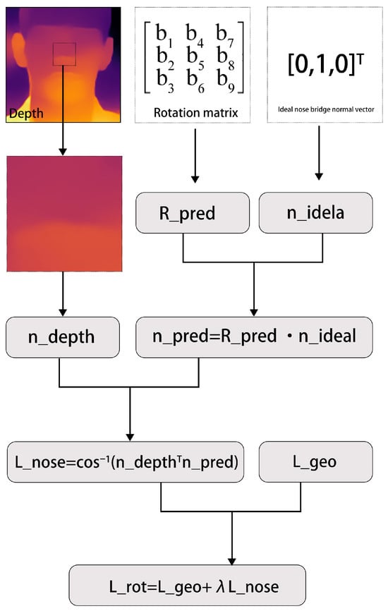
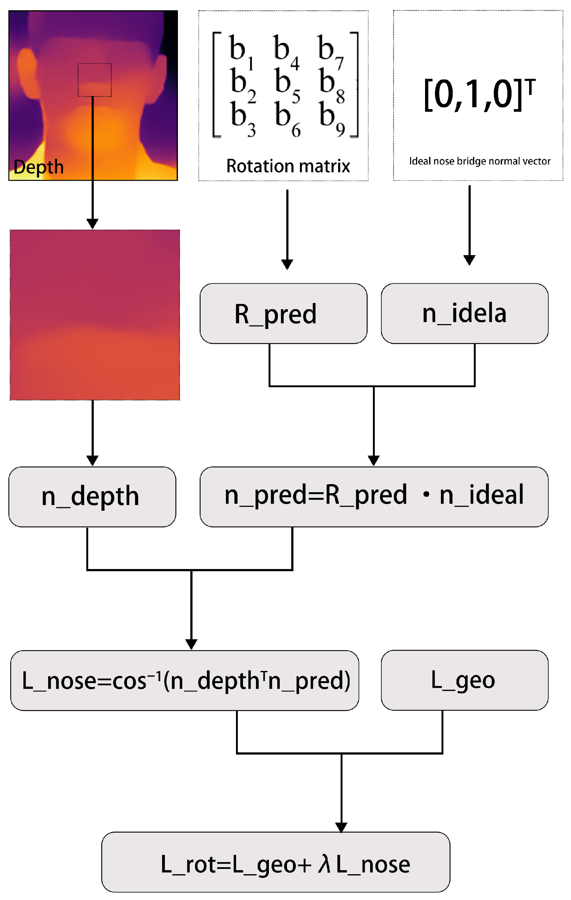
As shown in Figure 3, ${\mathbf{R}}_{\mathrm{pred}}$ is the predicted rotation matrix, and ${\mathbf{R}}_{\mathrm{GT}}$ is the ground-truth rotation matrix.

Figure 3. The process integrates data from a depth map of the nose bridge area and a predicted rotation matrix. These inputs are processed in parallel to generate two distinct normal vectors, which are then compared to calculate an angular loss. Finally, this loss is combined with a separate geometric loss to produce the total loss for model training.

Nasal Bridge Normal Constraint. The method focuses on the nasal bridge region of the face, which is relatively stable in structure and has a clear directionality. We operationally define it as a rectangular image area of pixels centered on the nose tip point. The key insight is that we can compute the surface-normal vector from the depth map in two ways: (1) directly from the depth gradients in the image space, and (2) by transforming the ideal nasal bridge normal vector using the predicted rotation matrix. If the rotation prediction is correct, these two normal vectors should align.

Specifically, within the nasal bridge region, we use the gradient information of the input depth map to calculate the average normal vector of this local surface, denoted as ${\mathbf{n}}_{\mathrm{depth}}$. This represents the actual geometric orientation observed in the depth data. Simultaneously, based on the currently predicted head rotation matrix, we can derive the ideal normal vector direction of the nasal bridge in the head coordinate system:

$${\mathbf{n}}_{\mathrm{pred}}={\mathbf{R}}_{\mathrm{pred}}·{\mathbf{n}}_{\mathrm{ideal}}$$

(10)

where ${\mathbf{n}}_{\mathrm{ideal}}={[0,1,0]}^T$ is the ideal nasal bridge normal vector.

Direction Alignment Loss. To incorporate anatomical knowledge into the optimization process, we design a direction alignment function ${\mathcal{L}}_{\mathrm{nose}}$. The core goal of this loss function is to force ${\mathbf{n}}_{\mathrm{depth}}$ and ${\mathbf{n}}_{\mathrm{pred}}$ to align as much as possible. When these two normal vectors point in the same direction, it indicates that the predicted rotation correctly captures the geometric structure of the nasal bridge. The loss is calculated by measuring the angle between these two unit normal vectors, specifically expressed as

$${\mathcal{L}}_{\mathrm{nose}}={cos}^{-1}\left({\mathbf{n}}_{\mathrm{depth}}^T{\mathbf{n}}_{\mathrm{pred}}\right)$$

(11)

When the directions are consistent, the dot product is 1, and the loss is 0; the greater the directional deviation, the larger the loss value.

Factors affecting the nasal bridge normal and ${\mathcal{L}}_{\mathrm{nose}}$. The loss depends on ${\mathbf{n}}_{\mathrm{depth}}$ obtained from finite differences on the depth patch, so it inherits the limitations of monocular depth: sensor or pseudo-depth noise inflates gradient error and can bias ${\mathbf{n}}_{\mathrm{depth}}$; occlusion or missing data in the nasal region makes the crop unreliable; and inter-person shape variability changes local surface orientation even at similar poses. These effects do not invalidate the constraint but imply that ${\mathcal{L}}_{\mathrm{nose}}$ is most trustworthy when the bridge is visible and depth is locally coherent—precisely the regime we target with adaptive gating below. The geodesic term ${\mathcal{L}}_{\mathrm{geo}}$ remains the primary objective when local geometry is untrustworthy.

Design scope and extension beyond a single region. Equations (10)–(12) instantiate a reusable local normal–rotation consistency template: choose a facial crop $\mathcal{R}$, estimate a unit normal ${\mathbf{n}}_{\mathrm{depth}}$ from depth gradients on $\mathcal{R}$, specify a head-fixed reference direction ${\mathbf{n}}_{\mathrm{ideal}}$ for that patch, and penalize the angle between ${\mathbf{n}}_{\mathrm{depth}}$ and ${\mathbf{R}}_{\mathrm{pred}}{\mathbf{n}}_{\mathrm{ideal}}$. The nasal bridge is our primary choice because it combines relatively rigid anatomy, frequent visibility in near-frontal views (where the constraint is active), and depth discontinuities that stabilize finite-difference normals. Conceptually, the same construction applies to other rigid, depth-stable areas (e.g., forehead or chin regions) after defining appropriate $\mathcal{R}$, ${\mathbf{n}}_{\mathrm{ideal}}$, and viewpoint gating; multi-patch aggregation is deferred to future work. We therefore view the methodological contribution as the consistency mechanism linking depth observables to SO(3) predictions, rather than an assertion that only the nasal bridge is usable.

Composite Loss Function. Finally, to comprehensively optimize the overall accuracy of the rotation matrix and the anatomical consistency of the nasal bridge region, we fuse this newly introduced nasal bridge normal loss ${\mathcal{L}}_{\mathrm{nose}}$ with the standard geodesic loss ${\mathcal{L}}_{\mathrm{geo}}$. The geodesic loss ensures global rotation accuracy, while the nasal bridge loss provides local geometric constraints. The fusion method uses a weighted sum:

$${\mathcal{L}}_{\mathrm{rot}}={\mathcal{L}}_{\mathrm{geo}}+\lambda {\mathcal{L}}_{\mathrm{nose}}$$

(12)

where $\lambda$ is a pose-dependent adaptive coefficient used to balance the relative importance of the two losses in the total optimization objective. We note that the supervision signal itself may have inherent limitations. For instance, when viewing the nasal bridge from a side angle, the actual ground-truth normal vector derived from the depth map in this region may not align with the idealized vector ${[0,1,0]}^T$. This inconsistency could potentially mislead the training process. Specifically, when the head pose approaches a side view, the nasal bridge region may become occluded or deformed, leading to unreliable computations. To address this issue, we make $\lambda$ a pose-dependent adaptive parameter. We set $\lambda$ to its default value when $|{\theta }_{\mathrm{yaw}}|\le {\theta }_{\mathrm{th}}={45}^{\circ }$, and $\lambda =0$ when $|{\theta }_{\mathrm{yaw}}|>{\theta }_{\mathrm{th}}$ so that the nasal loss is disabled in large-profile views. Here ${\theta }_{\mathrm{yaw}}$ is the predicted yaw from the same forward pass as ${\mathbf{R}}_{\mathrm{pred}}$, so gating remains differentiable; gating on ground-truth yaw is an alternative that can stabilize early training at the cost of train–test mismatch, and we report the predicted-yaw variant unless noted.

On the yaw threshold ${\theta }_{\mathrm{th}}={45}^{\circ }$. This value is a pragmatic heuristic, not a uniquely optimal constant: it marks a regime where the frontal nasal bridge model and stable depth gradients are less reliable. We selected ${45}^{\circ }$ as a compromise between retaining the constraint for near-frontal and mild profile views (where Table 6 shows strong behavior in the frontal and semi-profile bins) and disabling it before large-profile errors dominate. Indirect empirical support comes from the $\lambda$ ablation (Table 4): $\lambda =0$ degrades overall MAE versus $\lambda =0.3$, showing that the constraint helps when used selectively, while excessive $\lambda$ hurts—consistent with the need to turn off misleading supervision at challenging viewpoints. A dense sweep of ${\theta }_{\mathrm{th}}$ would be informative but is left for future work; the qualitative behavior across yaw bins in Figure 4 and Table 6 contextualizes performance where the nasal loss is inactive.

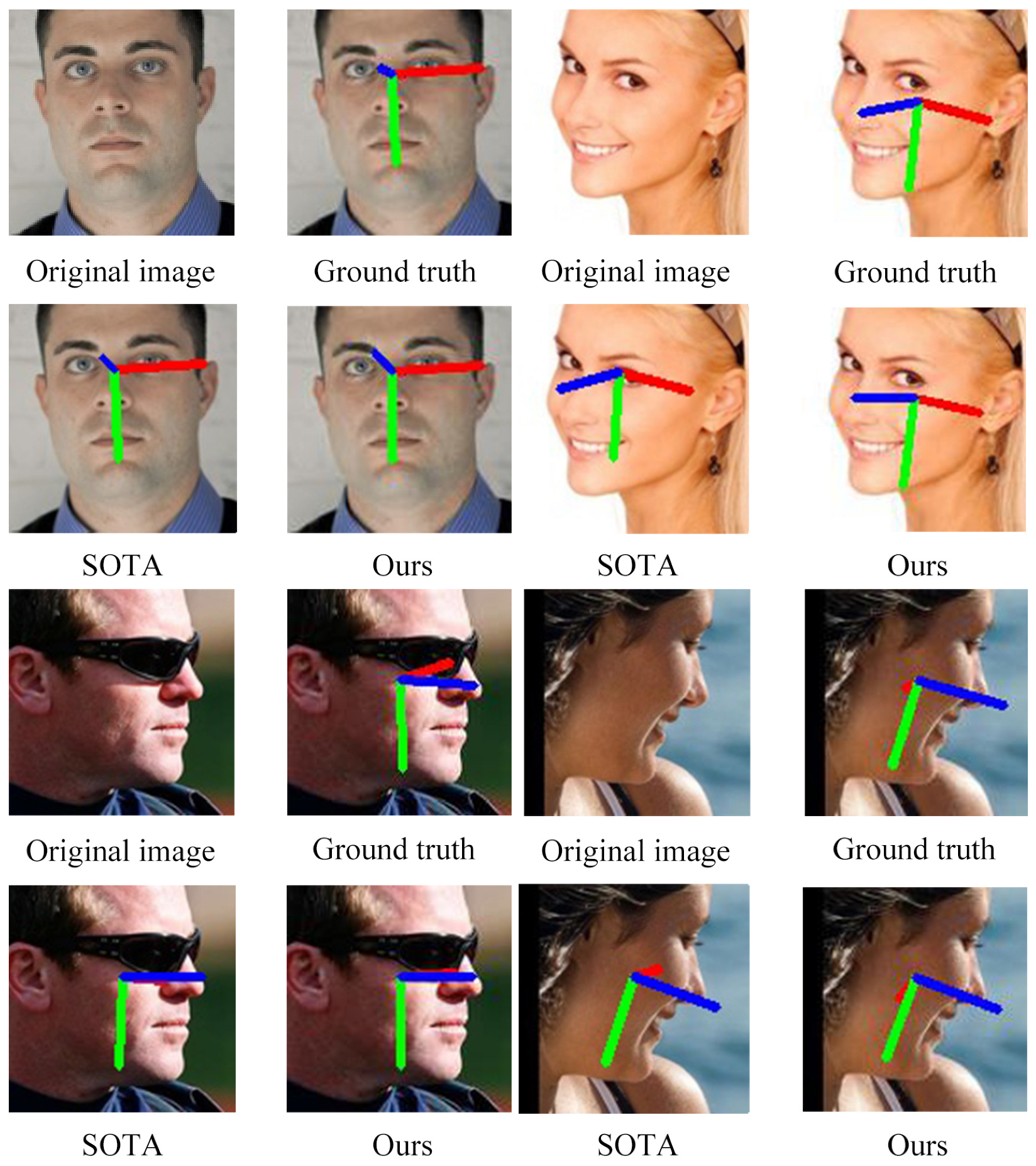
Figure 4. Qualitative comparison of head pose estimation results across different yaw angle ranges. The figure is organized in a 2 × 2 grid: (top-left) frontal views with yaw $<{30}^{\circ }$, showing the original image, ground-truth pose, SOTA method prediction, and our method’s prediction; (top-right) semi-profile views with yaw between ${30}^{\circ }$ and ${60}^{\circ }$, displaying the same four components; (bottom-left) profile views with yaw between ${60}^{\circ }$ and ${90}^{\circ }$; (bottom-right) extreme profile views with yaw $>{90}^{\circ }$. Each subfigure shows predicted poses over large viewing angles; quantitative accuracy is reported separately (Table 2 and yaw-stratified Table 6). The colored short axes indicate rotation directions: red line (X-axis) mainly denotes yaw (left/right head turning), green line (Y-axis) mainly denotes pitch (up/down head motion), and blue line (Z-axis) mainly denotes roll (head tilting).

By minimizing this composite loss function ${\mathcal{L}}_{\mathrm{rot}}$, the model can effectively utilize the geometric features of the nasal bridge region for regularization constraints while learning the overall head pose, thereby improving rotation estimation accuracy (MAE under the protocol in Section 4). Qualitative comparisons across yaw angle ranges (from frontal views to extreme profile views with yaw $>{90}^{\circ }$) are shown in Figure 4; they complement global MAE and illustrate accuracy on challenging poses in those views, not a separate “robustness” metric.

4. Experiments and Analysis

This experiment uses RepVGG-D2se as the backbone network, introducing a self-attention mechanism to enhance feature extraction capability. The training phase adopts a multi-branch structure to improve performance and converts to an efficient single-path inference mode during deployment through structural re-parameterization. To address the lack of depth in training data, normalization and center cropping preprocessing methods are used, combined with MTCNN [39] to generate complete samples. The network is trained for 70 epochs using the Adam optimizer with phased learning rate scheduling. Full hyperparameters, random seed, MiDaS settings, statistical reporting, and a discussion of fair comparison against RGB-only baselines are consolidated in Section 4.2. This solution significantly improves inference efficiency while maintaining accuracy.

4.1. Dataset Initialization

Current mainstream head pose datasets are limited by their annotation methods and generally suffer from pose distribution bias, with most samples concentrated near frontal face angles. To ensure the objectivity and comparability of the evaluation, we strictly followed domain specifications and conducted comprehensive tests on three widely recognized public datasets.

300W-LP [14]: This dataset integrates about 4000 real face images from multiple databases, generating about 66,225 synthetic face samples through algorithms, and further expands to 122,450 samples using image flipping technology. The annotation information is provided in the form of Euler angles (we convert them into rotation matrices during training). Since the original dataset does not contain depth information, we use the MiDaS monocular depth estimation algorithm to generate corresponding depth maps for all samples. The generated depth maps are normalized using per-image min–max normalization to the range [0, 1] to ensure scale invariance and stable training dynamics (see Section 3.1 for rationale and limitations of this choice).

AFLW2000 [16]: This dataset contains the first 2000 images of the AFLW dataset, providing accurate annotations including real 3D face models and 68 key points. This dataset is characterized by a large range of pose variations and complex occlusion scenes, making it suitable for cropping face regions for pose estimation. Similar to 300W-LP, this dataset also lacks original depth data, so the MiDaS algorithm is also used to generate depth maps, which are subsequently normalized using the same min–max normalization strategy (Section 3.1).

BIWI [15]: This dataset was collected in a controlled laboratory environment, containing 15,678 images of 20 subjects. Its characteristic is that the head region occupies a relatively small proportion in the image, so we use the MTCNN [39] face detector for loose head region cropping to effectively extract the main body of the head. The BIWI dataset comes with its own depth images, which provides an important data foundation for this research. To maintain consistency with the other datasets, the original depth images from BIWI are also normalized to the range [0, 1] using the same min–max normalization approach.

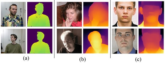
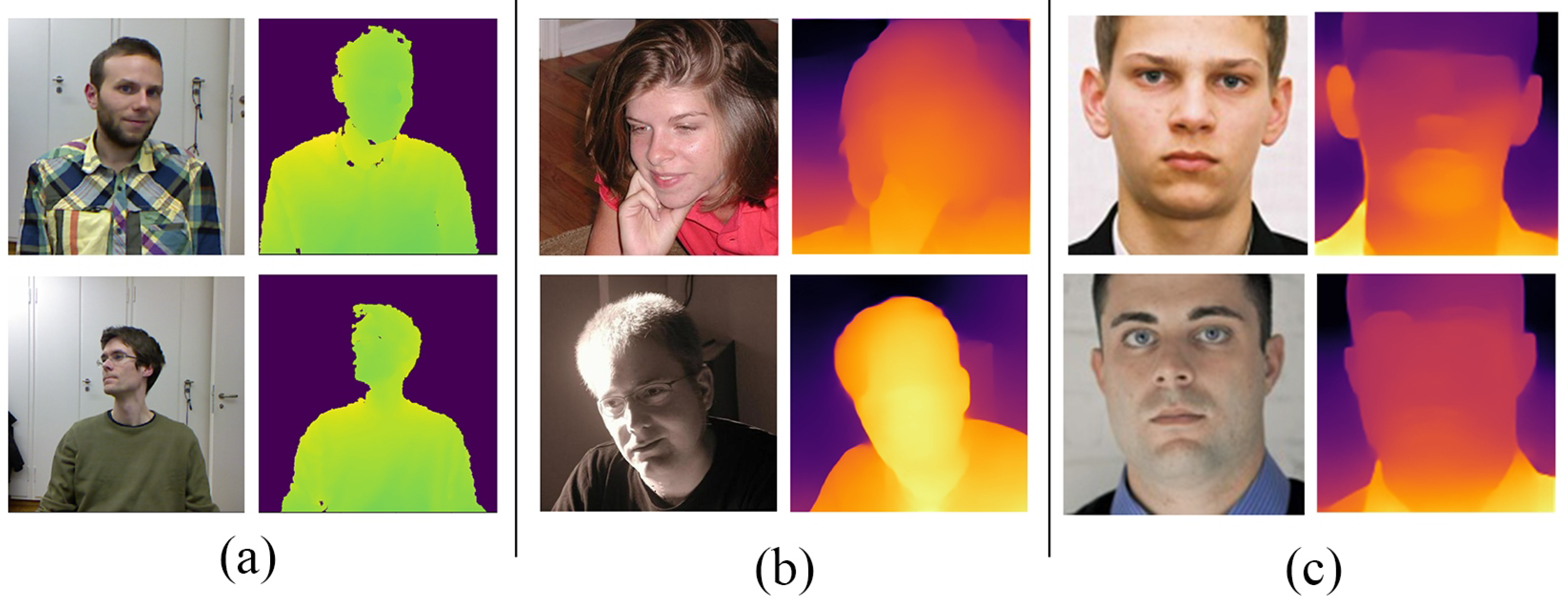
After the above data preprocessing flow (including face/head center cropping, depth map generation/use, pose selection), we finally obtained standardized preprocessing results for the three datasets: face-center-aligned cropped RGB images and their corresponding depth images of consistent size, as shown in Figure 5.

Figure 5. Display of facial images and their corresponding depth maps from three datasets: BIWI (a), AFLW2000 (b), and 300W_LP (c). Each dataset displays two examples, and the depth map uses color coding to represent depth information (warmer tones represent closer areas).

4.2. Evaluation Protocol, Fair Comparison, and Reproducibility

Standard evaluation protocol. We follow the widely adopted training and testing split: models are trained only on 300W-LP and evaluated on the full BIWI and AFLW2000 test sets, consistent with prior landmark-free head pose work [13,14,15,16]. Predicted rotation matrices are converted to Euler angles (yaw, pitch, roll), and we report mean absolute error (MAE) in degrees for each angle and for the average over the three angles, matching the metrics used by the baselines cited in Table 2.

Yaw, pitch, roll vs. overall MAE. The same error statistic is used throughout: absolute angular error in degrees. For each test sample and each axis $a\in \{\mathrm{yaw},\mathrm{pitch},\mathrm{roll}\}$, we compute $|{\widehat{\theta }}_a-{\theta }_a^{\mathrm{GT}}|$. Per-axis MAE is the mean of these absolute errors over the test set for that axis only. The overall MAE column is not a separate formula: it is the arithmetic mean of the three per-axis MAEs, $({\mathrm{MAE}}_{\mathrm{yaw}}+{\mathrm{MAE}}_{\mathrm{pitch}}+{\mathrm{MAE}}_{\mathrm{roll}})/3$; i.e., a single summary of the same three MAEs reported in the table.

Fairness of RGB–D versus RGB-only comparisons. Table 2 places our method next to published RGB-only models under the same protocol. This is useful for contextualizing accuracy but is not a strictly modality-matched benchmark: our pipeline consumes an additional depth channel (captured on BIWI or estimated by MiDaS on 300W-LP/AFLW2000), so improvements reflect both architectural choices and the availability of geometric cues. We address fairness as follows. (i) Internal controlled ablation: Table 5 toggles depth and SE within the same RepVGG-based training recipe, isolating the effect of depth fusion and attention relative to an RGB-only configuration of our network. (ii) Cost and assumptions: Depth is fixed offline (MiDaS is not fine-tuned on head pose labels), so every compared method could in principle consume the same depth maps; we do not retrain every external baseline with identical depth inputs, which would require harmonized codebases and compute. (iii) Interpretation: We therefore emphasize protocol-aligned comparison in Table 2 and modality-controlled evidence in Table 5.

Statistical reporting. Tables 2–6 report point estimates from a single training run with fixed randomness (see below), which matches how several cited baselines report results without variance. Readers can reproduce the quoted numbers using the stated seed and hyperparameters; repeating training with alternative seeds is a straightforward extension for estimating confidence intervals, which we encourage for future community benchmarks.

Implementation details for reproducibility. The RGB branch uses RepVGG-D2se [38]; the depth branch follows the lightweight convolutional pipeline in Section 3.1. Crops are resized to $224\times 224$ pixels for RGB and depth (see Section 3.1 for aspect-ratio effects). Training employs the Adam optimizer (${\beta }_1=0.9$, ${\beta }_2=0.999$) for 70 epochs with batch size 64, weight decay ${10}^{-4}$, and an initial learning rate of ${10}^{-3}$ reduced by a factor of 10 at epochs 50 and 60 (phased schedule). The SE reduction ratio is $r=16$ on both branches. The anatomical loss uses $\lambda =0.3$ when $|{\theta }_{\mathrm{yaw}}| \le {45}^{\circ }$ and $\lambda =0$ otherwise, as in Section 3.2. For 300W-LP and AFLW2000, depth maps are generated offline with the publicly released DPT-based MiDaS weights [40] (ICCV 2021 MiDaS family) using default inference settings and without fine-tuning on pose data, then per-image min–max normalized as in Section 3.1; BIWI uses dataset depth with the same normalization. Domain note: MiDaS is trained on diverse in-the-wild scenes, not on head-only crops; residual domain shift between pseudo-depth and real sensor depth on BIWI is expected and is partially mitigated by per-image normalization and joint training with RGB, but not eliminated. MTCNN [39] is applied for detection and cropping where described in Section 4. We set the random seed to 42 for the reported runs. Experiments were executed on a Linux workstation with an NVIDIA GeForce RTX 4090 GPU. A full training run of 70 epochs under the hyperparameters above takes approximately 24 h wall-clock time on this hardware.

4.3. Pose Estimation Performance Verification

Following the standard evaluation protocol in the field, the model was trained on the synthetic dataset 300W-LP and its generalization performance was tested on the real-world datasets BIWI and AFLW2000. To maintain metric consistency, the predicted 6D rotation matrices were converted to Euler angles, with the mean absolute error (MAE) serving as the evaluation metric. The modality assumptions and reproducibility settings are detailed in Section 4.2. As shown in Table 2, Deep6DHead achieves the lowest roll MAE among the listed methods on both datasets. Overall MAE is slightly better than 6DRepNet [13] on BIWI ($-0.{02}^{\circ }$) and AFLW2000 ($-0.{35}^{\circ }$ in $\mathrm{\Delta }$), while yaw and pitch remain higher than some RGB-only entries (e.g., 6DRepNet on BIWI yaw). The qualitative results in Figure 4 illustrate behavior across a wide range of head poses, from frontal views to extreme profile angles exceeding ${90}^{\circ }$.

Table 2. Comparison with state-of-the-art methods on BIWI and AFLW2000 under the standard 300W-LP training protocol. All errors are MAE in degrees. Euler angles follow the usual yaw–pitch–roll convention after converting each predicted rotation matrix to angles as in the cited baselines. Δ is overall MAE minus that of 6DRepNet [13] on the same dataset (negative means lower error than 6DRepNet). Listed baselines are RGB-only from the literature; our method uses additional depth (Section 4.2).

Method	BIWI					AFLW2000
	Yaw	Pitch	Roll	MAE	Δ	Yaw	Pitch	Roll	MAE	Δ
WHENet [23]	3.99	4.39	3.06	3.81	+0.34	5.11	6.24	4.92	5.42	+1.45
6DRepNet [13]	3.24	4.48	2.68	3.47	0.00	3.63	4.91	3.37	3.97	0.00
2DHeadPose [41]	3.81	3.78	2.73	3.44	−0.03	2.85	4.47	2.82	3.38	−0.59
TokenHPE [28]	3.95	4.51	2.71	3.72	+0.25	4.36	5.54	4.08	4.66	+0.69
HeadDiff [17]	3.47	4.20	2.71	3.46	−0.01	3.15	4.55	4.08	3.57	−0.40
LightNet [42]	3.26	3.15	2.97	3.35	−0.12	-	-	-	-	-
WQuatNet [43]	3.91	4.20	2.64	3.58	+0.11	3.39	4.62	3.23	3.75	−0.22
Deep6DHead (Ours)	4.23	4.07	2.05	3.45	−0.02	3.53	4.53	2.80	3.62	−0.35

4.4. Validation of the Optimization Loss with Anatomical Constraints

To overcome the limitations of the pure geodesic loss ${\mathcal{L}}_{\mathrm{geo}}$, in terms of rotation matrix orthogonality and local geometric consistency, this work introduces an anatomical loss based on the nasal bridge normal ${\mathcal{L}}_{\mathrm{nose}}$, constructing a composite loss function ${\mathcal{L}}_{\mathrm{rot}}={\mathcal{L}}_{\mathrm{geo}}+\lambda {\mathcal{L}}_{\mathrm{nose}}$. This design forces the predicted rotation direction to align with the local surface geometry, imposing biomechanically plausible constraints on the network. As shown in Table 3, under the same network architecture and training conditions, the composite loss ${\mathcal{L}}_{\mathrm{rot}}$ significantly reduces the MAE on the BIWI test set to 3.45. This result validates the effectiveness of the anatomy-driven constraint in correcting the geometric deviations of the rotation matrix.

Table 3. Comparison between the geodesic loss (${\mathcal{L}}_{\mathrm{geo}}$) and the composite loss (${\mathcal{L}}_{\mathrm{rot}}$).

Loss Function	BIWI				AFLW2000
	Yaw	Pitch	Roll	MAE	Yaw	Pitch	Roll	MAE
${\mathcal{L}}_{\mathrm{geo}}$	4.75	4.86	2.16	3.92	3.45	5.46	3.66	4.19
${\mathcal{L}}_{\mathrm{rot}}$	4.23	4.07	2.05	3.45	3.53	4.53	2.80	3.62

To delve into the impact mechanism of anatomical constraint strength on model performance, we conducted an ablation study on the hyperparameter $\lambda$. A clear trend of performance change was observed on both the BIWI and AFLW2000 datasets: when $\lambda$ was in the range of 0.1–0.3, the overall MAE showed a significant downward trend. Specifically, with $\lambda =0.3$, the MAE on the BIWI dataset reached an optimal value of 3.45, while on the AFLW2000 dataset, it decreased to 3.62, as shown in Table 4. However, excessively strong constraints ($\lambda \ge 0.3$) were found to impair generalization ability by overfitting the local nasal bridge features. Consequently, $\lambda =0.3$ was selected as the operating point of the model, as this configuration achieves the optimal synergistic balance between geometric accuracy and anatomical plausibility with minimal computational overhead.

Table 4. Ablation study results of the hyperparameter $\lambda$.

$\mathit{\lambda }$	BIWI				AFLW2000
	Yaw	Pitch	Roll	MAE	Yaw	Pitch	Roll	MAE
0.0	4.58	5.95	3.45	4.66	3.98	5.98	4.71	4.89
0.1	4.36	5.18	2.75	4.10	3.74	5.28	3.76	4.26
0.3	4.23	4.07	2.05	3.45	3.53	4.53	2.80	3.62
0.5	5.52	5.63	3.13	4.76	3.68	6.64	4.71	5.01
1.0	6.30	9.82	6.95	7.69	4.24	10.48	9.49	8.07

The composite loss in Equation (12) is not a sum of two unrelated objectives. The geodesic term ${\mathcal{L}}_{\mathrm{geo}}$ minimizes the angular error between ${\mathbf{R}}_{\mathrm{pred}}$ and the supervised rotation ${\mathbf{R}}_{\mathrm{GT}}$, while ${\mathcal{L}}_{\mathrm{nose}}$ pulls ${\mathbf{R}}_{\mathrm{pred}}$ toward consistency between depth-derived normals and the head-frame bridge direction. When monocular depth is noisy or the bridge patch is a poor match to the idealized model, gradients from ${\mathcal{L}}_{\mathrm{nose}}$ can oppose those from ${\mathcal{L}}_{\mathrm{geo}}$, so increasing $\lambda$ does not monotonically improve accuracy. Table 4 reflects this coupling: moderate $\lambda$ improves MAE relative to $\lambda =0$, but large $\lambda$ sharply worsens results—consistent with the anatomical term dominating and overfitting local depth artifacts. Table 3 complements this by isolating the effect of removing ${\mathcal{L}}_{\mathrm{nose}}$ entirely while keeping ${\mathcal{L}}_{\mathrm{geo}}$. Together, Table 3 and Table 4 provide an ablation over how strongly the two terms are tied, which is the relevant notion of interaction for our additive formulation.

This revision emphasizes final validation accuracy under controlled ablations (same backbone, schedule, and seed; only the loss composition or $\lambda$ changes). We do not include epoch-wise plots of ${\mathcal{L}}_{\mathrm{geo}}$, ${\mathcal{L}}_{\mathrm{nose}}$, or their sum, because the reviewer-requested evidence for component contribution is already visible in the end-point comparisons: Table 3 shows the geodesic-only baseline versus the composite loss, and Table 4 traces how varying $\lambda$ shifts the balance between the two gradients. The poor MAE at $\lambda =1.0$ supports the interaction narrative above (conflicting or over-strong anatomical supervision) without requiring per-epoch curves. Future work may log the two losses separately for each epoch to visualize transient trade-offs during optimization; that analysis is orthogonal to the design choices validated here.

4.5. Ablation Study on the Depth-Attention Mechanism

We ablate depth and SE inside the same RepVGG training recipe (Table 5). SE performs squeeze–excitation channel recalibration on each branch before fusion; depth supplies geometric contrast that RGB-only RepVGG does not see. Per-branch SE pre-conditions depth and RGB features; the concatenation of $v_d$ and $v_{\mathrm{rgb}}$ and the FC rotation head then combine modalities for pose. Raw depth noise is partially suppressed when SE down-weights unreliable channels. Table 5 shows that removing either depth or SE hurts MAE relative to the full model; depth-only or SE-only configurations are not sufficient in isolation.

Table 5. Ablation study on the depth-attention mechanism.

Backbone	SE Module	Depth	BIWI				AFLW2000
			Yaw	Pitch	Roll	MAE	Yaw	Pitch	Roll	MAE
RepVGG	No	No	3.24	4.48	2.68	3.47	3.63	4.91	3.37	3.97
RepVGG	No	Yes	7.24	6.94	3.70	5.96	4.28	5.48	3.84	4.53
RepVGG	Yes	No	6.56	6.60	3.98	5.71	4.38	4.72	3.56	4.22
RepVGG-D2se	Yes	Yes	4.23	4.07	2.05	3.45	3.53	4.53	2.80	3.62

4.6. Stratified Evaluation Under Challenging Poses

We complement the global MAE in Table 2 with yaw-stratified MAE and qualitative visualization, i.e., accuracy on challenging poses in stratified evaluation rather than a separate “robustness” index.

Stratified MAE by yaw range. We evaluate the model across pose angle ranges as follows. The test samples from BIWI and AFLW2000 are partitioned into four groups based on the absolute ground-truth yaw angle: frontal ($|{\theta }_{\mathrm{yaw}}| \le {30}^{\circ }$), semi-profile (${30}^{\circ } < \left|{\theta }_{\mathrm{yaw}}\right| \le {60}^{\circ }$), profile (${60}^{\circ }<\left|{\theta }_{\mathrm{yaw}}\right| \le {90}^{\circ }$), and extreme profile ($|{\theta }_{\mathrm{yaw}}| > {90}^{\circ }$). Sample counts per bin are imbalanced (most faces are near-frontal in these benchmarks); Table 6 should therefore be read as a stratified diagnostic, not a balanced per-bin contest. We do not tabulate 6DRepNet [13] per bin here; Table 2 gives protocol-matched overall metrics for direct comparison. As shown in Table 6, our method maintains relatively stable performance across pose ranges. Notably, the performance degradation in extreme profile views (>${90}^{\circ }$) is moderate, with MAE increasing from 3.45 to 4.75 on BIWI, consistent with the adaptive $\lambda$ mechanism that disables the nasal bridge constraint when predicted yaw exceeds ${45}^{\circ }$. Depth provides geometric cues when facial appearance is weak, complementing RGB.

Link to anatomical loss gating. Table 6 should be read together with the anatomical discussion in Section 3.2: bins with smaller $|{\theta }_{\mathrm{yaw}}|$ are where ${\mathcal{L}}_{\mathrm{nose}}$ is typically active ($\lambda >0$), whereas large-profile bins rely more on ${\mathcal{L}}_{\mathrm{geo}}$ and RGB–D features because $\lambda =0$. This stratification does not isolate depth noise or occlusion as separate controlled factors—AFLW2000 in particular contains challenging appearances—but it does show that residual accuracy remains reasonable when the nasal constraint is largely off. Combined with the $\lambda$ ablation (Table 4), this supports the design choice to gate the anatomical term rather than apply it uniformly.

Table 6. Performance stratified by ground-truth $\left|yaw\right|$ (degrees). MAE in degrees; bins are imbalanced (see text).

Pose Range	BIWI				AFLW2000
	Yaw	Pitch	Roll	MAE	Yaw	Pitch	Roll	MAE
Frontal ($\left|\theta \right|\le {30}^{\circ }$)	3.85	3.92	1.95	3.24	3.12	4.28	2.65	3.35
Semi-profile (${30}^{\circ }<\left|\theta \right|\le {60}^{\circ }$)	4.15	4.12	2.08	3.45	3.58	4.55	2.82	3.65
Profile (${60}^{\circ }<\left|\theta \right|\le {90}^{\circ }$)	4.68	4.35	2.25	3.76	4.12	4.88	3.15	4.05
Extreme ($\left|\theta \right|>{90}^{\circ }$)	5.45	5.28	3.52	4.75	4.85	5.65	4.25	4.92

Table 6. Performance stratified by ground-truth $\left|yaw\right|$ (degrees). MAE in degrees; bins are imbalanced (see text).

Pose Range	BIWI				AFLW2000
	Yaw	Pitch	Roll	MAE	Yaw	Pitch	Roll	MAE
Frontal ($\left|\theta \right|\le {30}^{\circ }$)	3.85	3.92	1.95	3.24	3.12	4.28	2.65	3.35
Semi-profile (${30}^{\circ }<\left|\theta \right|\le {60}^{\circ }$)	4.15	4.12	2.08	3.45	3.58	4.55	2.82	3.65
Profile (${60}^{\circ }<\left|\theta \right|\le {90}^{\circ }$)	4.68	4.35	2.25	3.76	4.12	4.88	3.15	4.05
Extreme ($\left|\theta \right|>{90}^{\circ }$)	5.45	5.28	3.52	4.75	4.85	5.65	4.25	4.92

5. Discussion

Although Deep6DHead improves roll MAE and overall MAE versus 6DRepNet on the standard protocol (Table 2), yaw and pitch are not uniformly best among listed RGB-only methods: the nasal bridge loss targets geometry that aligns most directly with roll-like behavior, while global yaw/pitch benefit more from appearance and dataset bias. The method also depends on depth or pseudo-depth quality; severe occlusion can remove reliable facial structure, and MiDaS depth on in-the-wild crops does not match the sensor depth on BIWI without a domain gap.

Outlook. Fully unconstrained deployment (motion blur, demographics, heavy occlusion) motivates cross-domain depth adaptation, multi-region anatomical terms, and calibrated rotation uncertainty. Lightweight backbones and depth-free fallbacks remain important for embedded use. Future work may combine temporal or inertial cues when latency and privacy constraints allow.

6. Conclusions

This paper presented Deep6DHead, a landmark-free RGB–D head pose estimator that couples RepVGG-D2se dual-branch encoding with SE recalibration, 6D rotation regression [13], and a yaw-gated nasal bridge normal loss on pseudo-depth (MiDaS [44]) or sensor depth. On BIWI and AFLW2000 under training on 300W-LP, the model achieves the lowest roll MAE among the compared entries in Table 2 and modest overall MAE gains versus 6DRepNet, with trade-offs on yaw and pitch relative to some RGB-only baselines. The central contribution is the depth–anatomy consistency mechanism; SE, fusion, and 6D heads are standard components used as engineered building blocks.

References

- Ritthipravat, P.; Chotikkakamthorn, K.; Lie, W.N.; Kusakunniran, W.; Tuakta, P.; Benjapornlert, P. Deep-learning-based head pose estimation from a single RGB image and its application to medical CROM measurement. Multimed. Tools Appl. 2024, 83, 77009–77028. [Google Scholar] [CrossRef] [Scilit]
- Murphy-Chutorian, E.; Doshi, A.; Trivedi, M.M. Head pose estimation for driver assistance systems: A robust algorithm and experimental evaluation. In Proceedings of the 2007 IEEE Intelligent Transportation Systems Conference, Bellevue, WA, USA, 30 September–3 October 2007; pp. 709–714. [Google Scholar]
- Murphy-Chutorian, E.; Trivedi, M.M. Head pose estimation and augmented reality tracking: An integrated system and evaluation for monitoring driver awareness. In IEEE Transactions on Intelligent Transportation Systems; IEEE: New York, NY, USA, 2010; Volume 11, pp. 300–311. [Google Scholar]
- Strazdas, D.; Hintz, J.; Al-Hamadi, A. Robo-hud: Interaction concept for contactless operation of industrial cobotic systems. Appl. Sci. 2021, 11, 5366. [Google Scholar] [CrossRef] [Scilit]
- Werner, P.; Saxen, F.; Al-Hamadi, A. Landmark based head pose estimation benchmark and method. In Proceedings of the 2017 IEEE International Conference on Image Processing (ICIP), Beijing, China, 17–20 September 2017; pp. 3909–3913. [Google Scholar]
- Bulat, A.; Tzimiropoulos, G. How far are we from solving the 2D & 3D face alignment problem? (and a dataset of 230,000 3D facial landmarks). In Proceedings of the IEEE International Conference on Computer Vision (ICCV), Venice, Italy, 22–29 October 2017; pp. 1021–1030. [Google Scholar]
- Mo, S.; Miao, X. OsGG-Net: One-step graph generation network for unbiased head pose estimation. In Proceedings of the 29th ACM International Conference on Multimedia; Association for Computing Machinery: New York, NY, USA, 2021; pp. 2465–2473. [Google Scholar]
- Ruiz, N.; Chong, E.; Rehg, J.M. Fine-grained head pose estimation without keypoints. In Proceedings of the IEEE/CVF Conference on Computer Vision and Pattern Recognition (CVPR) Workshops, Salt Lake City, UT, USA, 18–22 June 2018; pp. 2074–2083. [Google Scholar]
- Zhang, H.; Wang, M.; Liu, Y.; Yuan, Y. FDN: Feature decoupling network for head pose estimation. Proc. AAAI Conf. Artif. Intell. 2020, 34, 12789–12796. [Google Scholar] [CrossRef] [Scilit]
- Bisogni, C.; Nappi, M.; Pero, C.; Ricciardi, S. FASHE: A fractal based strategy for head pose estimation. IEEE Trans. Image Process. 2021, 30, 3192–3203. [Google Scholar] [CrossRef] [Scilit] [PubMed]
- Yang, T.-Y.; Chen, Y.-T.; Lin, Y.-Y.; Chuang, Y.-Y. FSA-Net: Learning fine-grained structure aggregation for head pose estimation from a single image. In Proceedings of the IEEE/CVF Conference on Computer Vision and Pattern Recognition (CVPR), Long Beach, CA, USA, 15–20 June 2019; pp. 1087–1096. [Google Scholar]
- Fischler, M.A.; Bolles, R.C. Random sample consensus: A paradigm for model fitting with applications to image analysis and automated cartography. Commun. ACM 1981, 24, 381–395. [Google Scholar] [CrossRef] [Scilit]
- Hempel, T.; Abdelrahman, A.A.; Al-Hamadi, A. 6d Rotation Representation For Unconstrained Head Pose Estimation. In Proceedings of the 2022 IEEE International Conference on Image Processing (ICIP), Bordeaux, France, 16–19 October 2022; pp. 2496–2500. [Google Scholar]
- Zhu, X.; Lei, Z.; Liu, X.; Shi, H.; Li, S. Face alignment across large poses: A 3D solution. In Proceedings of the 2016 IEEE Conference on Computer Vision and Pattern Recognition (CVPR), Las Vegas, NV, USA, 27–30 June 2016; pp. 146–155. [Google Scholar]
- Fanelli, G.; Dantone, M.; Gall, J.; Fossati, A.; van Gool, L. Random forests for real time 3d face analysis. Int. J. Comput. Vis. 2013, 101, 437–458. [Google Scholar] [CrossRef] [Scilit]
- Zhu, X.; Lei, Z.; Yan, J.; Yi, D.; Li, S.Z. High-fidelity pose and expression normalization for face recognition in the wild. In Proceedings of the 2015 IEEE Conference on Computer Vision and Pattern Recognition (CVPR), Boston, MA, USA, 7–12 June 2015; pp. 787–796. [Google Scholar]
- Wang, Y.; Liu, H.; Feng, Y.; Li, Z.; Wu, X.; Zhu, C. HeadDiff: Exploring Rotation Uncertainty With Diffusion Models for Head Pose Estimation. IEEE Trans. Image Process. 2024, 33, 1868–1882. [Google Scholar] [CrossRef] [Scilit] [PubMed]
- Baltrušaitis, T.; Robinson, P.; Morency, L.-P. 3D constrained local model for rigid and non-rigid facial tracking. In Proceedings of the IEEE Conference on Computer Vision and Pattern Recognition, Providence, RI, USA, 16–21 June 2012; pp. 2610–2617. [Google Scholar]
- Ranjan, R.; Patel, V.M.; Chellappa, R. HyperFace: A deep multi-task learning framework for face detection, landmark localization, pose estimation, and gender recognition. IEEE Trans. Pattern Anal. Mach. Intell. 2019, 41, 121–135. [Google Scholar] [CrossRef] [Scilit] [PubMed]
- Valle, R.; Buenaposada, J.M.; Baumela, L. Multi-task head pose estimation in-the-wild. IEEE Trans. Pattern Anal. Mach. Intell. 2021, 43, 2874–2881. [Google Scholar] [CrossRef] [Scilit] [PubMed]
- Hsu, H.-W.; Wu, T.-Y.; Wan, S.; Wong, W.H.; Lee, C.-Y. QuatNet: Quaternion-based head pose estimation with multiregression loss. IEEE Trans. Multimed. 2019, 21, 1035–1046. [Google Scholar] [CrossRef] [Scilit]
- Albiero, V.; Chen, X.; Yin, X.; Pang, G.; Hassner, T. img2pose: Face alignment and detection via 6DoF, face pose estimation. In Proceedings of the IEEE/CVF Conference on Computer Vision and Pattern Recognition (CVPR), Nashville, TN, USA, 19–25 June 2021; pp. 7617–7627. [Google Scholar]
- Zhou, Y.; Gregson, J. Whenet: Real-time fine-grained estimation for wide range head pose. In Proceedings of the 31st British Machine Vision Conference 2020, BMVC 2020, Virtual Event, UK, 7–10 September 2020. [Google Scholar]
- Zhou, Y.; Barnes, C.; Lu, J.; Yang, J.; Li, H. On the continuity of rotation representations in neural networks. In Proceedings of the 2019 IEEE/CVF Conference on Computer Vision and Pattern Recognition (CVPR), Long Beach, CA, USA, 16–21 June 2019; pp. 5738–5746. [Google Scholar]
- Liu, H.; Fang, S.; Zhang, Z.; Li, D.; Lin, K.; Wang, J. MFDNet: Collaborative poses perception and matrix Fisher distribution for head pose estimation. IEEE Trans. Multimed. 2022, 24, 2449–2460. [Google Scholar] [CrossRef] [Scilit]
- Pan, L.; Ai, S.; Ren, Y.; Xu, Z. Self-paced deep regression forests with consideration on underrepresented examples. In Proceedings of the 16th European Conference Computer Vision (ECCV), Glasgow, UK, 23–28 August 2020; Springer: Cham, Switzerland, 2020; pp. 271–287. [Google Scholar]
- Cao, Z.; Liu, D.; Wang, Q.; Chen, Y. Towards unbiased label distribution learning for facial pose estimation using anisotropic spherical Gaussian. In Proceedings of the 17th European Conference on Computer Vision; Springer: Cham, Switzerland, 2022; pp. 737–753. [Google Scholar]
- Zhang, C.; Liu, H.; Deng, Y.; Xie, B.; Li, Y. Tokenhpe: Learning orientation tokens for efficient head pose estimation via transformers. In Proceedings of the IEEE/CVF Conference on Computer Vision and Pattern Recognition (CVPR), Vancouver, BC, Canada, 17–24 June 2023; pp. 8897–8906. [Google Scholar]
- Yu, Y.; Mora, K.A.F.; Odobez, J.-M. HeadFusion: 360 head pose tracking combining 3D morphable model and 3D reconstruction. IEEE Trans. Pattern Anal. Mach. Intell. 2018, 40, 2653–2667. [Google Scholar] [CrossRef] [Scilit] [PubMed]
- Guo, J.; Zhu, X.; Yang, Y.; Yang, F.; Lei, Z.; Li, S.Z. Towards fast, accurate and stable 3D dense face alignment. In Computer Vision—ECCV (Lecture Notes in Computer Science); Vedaldi, A., Bischof, H., Brox, T., Frahm, J.M., Eds.; Springer: Cham, Switzerland, 2020; Volume 12364. [Google Scholar]
- Wu, C.-Y.; Xu, Q.; Neumann, U. Synergy between 3DMM and 3D landmarks for accurate 3D facial geometry. In Proceedings of the International Conference on 3D Vision (3DV), Virtual, 1–3 December 2021; pp. 453–463. [Google Scholar]
- Martyniuk, T.; Kupyn, O.; Kurlyak, Y.; Krashenyi, I.; Matas, J.; Sharmanska, V. DAD-3DHeads: A large-scale dense, accurate and diverse dataset for 3D head alignment from a single image. In Proceedings of the IEEE/CVF Conference on Computer Vision and Pattern Recognition (CVPR), New Orleans, LA, USA, 18–24 June 2022; pp. 20910–20920. [Google Scholar]
- Prokudin, S.; Gehler, P.; Nowozin, S. Deep directional statistics: Pose estimation with uncertainty quantification. In Proceedings of European Conference on Computer Vision (ECCV), Munich, Germany, 8–14 September 2018; pp. 534–551. [Google Scholar]
- Deng, H.; Bui, M.; Navab, N.; Guibas, L.; Ilic, S.; Birdal, T. Deep Bingham networks: Dealing with uncertainty and ambiguity in pose estimation. Int. J. Comput. Vis. 2022, 130, 1627–1654. [Google Scholar] [CrossRef] [Scilit]
- Mohlin, D.; Sullivan, J.; Bianchi, G. Probabilistic orientation estimation with matrix Fisher distributions. Adv. Neural Inf. Process. Syst. 2020, 33, 4884–4893. [Google Scholar]
- Wu, Z.; Xiong, Y.; Yu, S.X.; Lin, D. Unsupervised feature learning via non-parametric instance discrimination. In Proceedings of the IEEE/CVF Conference on Computer Vision and Pattern Recognition, Salt Lake City, UT, USA, 18–22 June 2018; pp. 3733–3742. [Google Scholar]
- Yin, Y.; Wang, Y.; Wang, H.; Chen, B. A Laplace-inspired distribution on SO(3) for probabilistic rotation estimation. In Proceedings of the 11th International Conference on Learning Representations, Kigali, Rwanda, 1–5 May 2023. [Google Scholar]
- Ding, X.; Zhang, X.; Ma, N.; Han, J.; Ding, G.; Sun, J. RepVGG: Making VGG-style ConvNets Great Again. In Proceedings of the IEEE/CVF Conference on Computer Vision and Pattern Recognition (CVPR), Virtual, 19–25 June 2021; pp. 13733–13742. [Google Scholar]
- Zhang, K.; Zhang, Z.; Li, Z.; Qiao, Y. Joint face detection and alignment using multitask cascaded convolutional networks. IEEE Signal Process. Lett. 2016, 23, 1499–1503. [Google Scholar] [CrossRef] [Scilit]
- Ranftl, R.; Bochkovskiy, A.; Koltun, V. Vision Transformers for Dense Prediction. In Proceedings of the IEEE/CVF International Conference on Computer Vision (ICCV), Montreal, QC, Canada, 11–17 October 2021; pp. 12179–12188. [Google Scholar]
- Wang, Y.; Zhou, W.; Zhou, J. 2DHeadPose: A simple and effective annotation method for the head pose in RGB images and its dataset. Neural Netw. 2023, 160, 50–62. [Google Scholar] [CrossRef] [Scilit] [PubMed]
- Zheng, L.; Li, J.; Zhu, Z.; Ji, W. LightNet: A lightweight head pose estimation model for online education and its application to engagement assessment. J. King Saud Univ. Comput. Inf. Sci. 2025, 37, 166. [Google Scholar] [CrossRef] [Scilit]
- Algabri, R.; Shin, H.; Abdu, A.; Bae, J.H.; Lee, S. WQuatNet: Wide range quaternion-based head pose estimation. J. King Saud Univ. Comput. Inf. Sci. 2025, 37, 24. [Google Scholar] [CrossRef] [Scilit]
- Xu, X.; Gao, Y.; Yan, K.; Lin, X.; Zou, Q. Location-free Human Pose Estimation. arXiv 2022, arXiv:2205.12619. [Google Scholar] [CrossRef] [Scilit]
Disclaimer/Publisher’s Note: The statements, opinions and data contained in all publications are solely those of the individual author(s) and contributor(s) and not of MDPI and/or the editor(s). MDPI and/or the editor(s) disclaim responsibility for any injury to people or property resulting from any ideas, methods, instructions or products referred to in the content. |
© 2026 by the authors. Licensee MDPI, Basel, Switzerland. This article is an open access article distributed under the terms and conditions of the Creative Commons Attribution (CC BY) license.