


Abstract
Classical homogenization theory treats critical exponents as universal quantities depending only on spatial dimension, but recent evidence shows that this assumption fails for continuum composites once the mechanism of randomness generation is taken into account. We synthesize three complementary frameworks—structural approximation, structural sums, and self-similar renormalization—to develop a unified geometric theory of criticality in random composites. Dilute-regime expansions for the effective conductivity and shear modulus are expressed in terms of structural sums whose ensemble statistics depend sensitively on the randomness protocol. To bridge the dilute and critical regimes, we employ self-similar factor approximants, iterated-root approximants, additive approximants, and renormalization schemes based on minimal-difference and minimal-sensitivity conditions, combined with Borel summation. For maximally disordered protocols , the conductivity index s and the elasticity index S fall within comparable numerical ranges, indicating a shared geometric origin and spectral response to the continuous breaking of translational symmetry. A regular periodic arrangement of inclusions () possesses full discrete translational symmetry; as a stochastic protocol is applied ( increases), this symmetry is gradually degraded until statistical chaos is reached. For instance, the parameter can be considered as a time of stirring. During this evolution, the system traverses a continuous spectrum of critical indices, which encodes the geometric and topological memory of the initial ordered state. It is established that the classical “universality” of percolation corresponds to a fixed point within a broader manifold of protocol-dependent critical behaviors. The framework developed here provides a coherent basis for inverse design, diagnostics, and classification of random composites by their disorder history, offering a geometric alternative to the universality paradigm.
Keywords:
random composites; dynamical protocols; effective conductivity; structural approximation; graphene MSC:
74Q15; 05B40
1. Introduction
Symmetry and disorder are fundamental characteristics of physical systems that shape their macroscopic behavior across conductivity, elasticity, diffusion, and various physical phenomena [1,2,3,4,5,6,7,8]. This work is devoted to establishing a new association between the degree of order or disorder in a physical structure and its geometric characteristics, with particular emphasis on their influence on the critical exponent, one of the key parameters governing densely packed composites.
The present study is theoretical in nature and restricted to two-dimensional, doubly periodic composites of circular inclusions. All analytic constructions, structural sums, and renormalization procedures are formulated in this setting. This clarification has been added to avoid any ambiguity regarding the scope of the results.
For the first time, the critical exponent was calculated by J.B. Keller [9] in 1963 for a regular array of perfectly conducting disks. This conception was developed to a regular sphere array [9] and deterministic multiple locations of inclusions [10,11].
In classical lattice-based percolation theory, critical behavior near the percolation threshold is described by universal exponents that depend only on the spatial dimension [1,12,13,14,15]. Within this paradigm, the percolation threshold for the concentration of inclusions may vary with geometry and protocol [2,3], but the associated critical indices are assumed to be universal. However, continuum composites violate this assumption in a fundamental way. Their microstructures are not sampled from a single canonical ensemble but are generated by specific geometric or dynamical protocols. Each protocol, which produces stirring, shaking, settling, random sequential adsorption, or dilution, produces distinct patterns of short- and long-range correlations, gap distributions, and local coordination. As a result, the effective properties of the composite retain a memory of the disorder-generation mechanism.
This observation aligns with recent developments in continuum percolation and jamming, where protocol-induced correlations have been shown to influence transport and mechanical properties [3,16,17]. These studies reinforce the idea that universality may break down in continuum systems when the disorder-generation mechanism is not fixed.
It is important to emphasize that the notions of protocol and probabilistic distribution of inclusions have distinct meanings in the theory of dispersed composites. A probabilistic distribution of non-overlapping inclusions is defined at a fixed moment in time, when a collection of inclusions of prescribed shape is embedded into a host material. The protocol generates a statistical realizations of that distribution and matters most when concrete estimates of the effective properties and critical behavior in particular are of primary interest.
We highlight this distinction because it plays a central role in the present work: two different protocols may sample the same nominal distribution while producing different geometric statistics, gap networks, and ultimately different effective exponents.
For any intermediate value , infinitely many distributions of equal non-overlapping disks exist. In much of the engineering literature, however, all such probabilistic distributions are tacitly reduced to a single “random distribution,” in which the sole geometric parameter f is assumed to determine the macroscopic behavior of the microstructure in addition to the material constants. Typically, authors use the uniform non-overlapping distribution . In this setting, the effective material constants are properly defined as the mathematical expectation of the effective constants computed over all probabilistic events, that is, over all admissible configurations of inclusion locations.
The computation over all admissible inclusion locations can be performed using statistical simulations consistent with the prescribed theoretical distribution. A protocol denotes a precisely defined set of rules used to generate a statistical realization of a given probabilistic distribution. Various protocols may be used to construct a representative volume element (RVE). Such a protocol can be formulated for a fixed volume fraction f, either within the same probabilistic distribution or across different ones, to model processes that capture the various types of interactions between inclusions [18].
In this work, we treat a protocol as a dynamical rule that generates a trajectory in the space of admissible microstructures, with representing a disorder parameter such as stirring time, shaking amplitude, or number of RSA attempts. This viewpoint allows us to interpret the critical index as a functional rather than a universal constant.
In [19], Random Walks (RW) and Random Sequential Adsorption (RSA) were used to simulate the same random distribution of disks . The RW protocol models a dynamic evolution of inclusion positions. For example, random walks initialized from a hexagonal array were performed in order to obtain representative configurations of for a fixed concentration f. It was shown in [20] that different modifications of the RSA protocol can lead to different effective material constants. This observation highlights the relevance of studying jammed packing of hard particles [3,4], where protocols with gradually increasing f are applied to determine the set of attainable jammed configurations.
A separate question concerns the macroscopic anisotropy determined by the prescribed distribution and by the symmetry of protocol rules. Frequently, we have at our disposal pictures of heterogeneous media, not knowing a priori their macroscopic isotropy. The methods based on symmetric lattice [21] do not work for random media. A computationally effective criterion to study anisotropy by structural sums was developed in [20,22,23,24].
The diversity of probabilistic distributions and protocols leads to the suggestion that the effective properties of densely packed composites require a separate study of the critical exponent, which depends on distributions and protocols. It is supposed that the critical exponent, together with the critical fraction of touching inclusions, becomes the de facto parameters of densely packed composites.
Recent studies have shown that dilute-regime expansions for effective conductivity [23] and elasticity [20] can be expressed in terms of structural sums whose statistics depend sensitively on the randomness protocol. These structural sums encode geometric correlations and the distribution of narrow gaps, which dominate transport in the dense regime. When combined with self-similar renormalization techniques, these expansions reveal that the critical indices governing effective properties are not fixed constants of the embedding dimension but protocol-dependent quantities [20,23].
We emphasize that the indices extracted in this work are effective exponents obtained from resummed finite-order expansions. They are not necessarily asymptotic renormalization-group exponents. This distinction is important for interpreting the results.
This protocol dependence is clearly reflected in the numerical results. For conductivity, the stirring protocol produces critical indices for superconductivity in the range [25], reflecting the broad distribution of gap widths and the high degree of geometric disorder. For elasticity, the maximally disordered protocol yields an index S for the elastic shear modulus in a comparable numerical range, despite the different singularities governing local interactions. The proximity of s and S in the case of maximal disorder supports a unified geometric interpretation of criticality.
The interval is also consistent with many experimental and numerical studies of two-dimensional disordered conductors and soft materials [12,26]. An especially revealing case arises in the dilution protocol, where disks are removed at random from an initially ordered configuration. Unlike additive protocols, which generate disorder by adding or displacing inclusions, dilution degrades the structure by eliminating elements of the original periodic arrangement. This mechanism preserves short-range order while collapsing long-range connectivity, producing a qualitatively different evolution of the gap network. A striking consequence is that the critical index may fall below the classical lower bound of . Values do not appear in additive protocols, where geometric redundancy maintains stronger transport pathways. In contrast, dilution removes entire branches of the transport structure, sharply reducing the number of independent conductive routes.
Such values have not been observed experimentally and should be interpreted as theoretical predictions that may motivate new fabrication techniques capable of producing controlled removal of inclusions or engineered long-range correlations.
The upper part of the spectrum is equally significant. Existing protocols do not generate indices beyond the observed range for maximally disordered configurations. Values have not been produced by any of the established protocols examined in this work. Such values would require mechanisms that amplify geometric anisotropy, induce long-range correlations, or create highly nonuniform gap distributions not accessible through standard disorder-generation schemes. The possibility of therefore points towards new physics and motivates the search for novel randomness protocols. These ideas are discussed in Section 10, where we outline how extending the upper end of the spectrum may reveal previously unknown geometric regimes.
As with the lower bound, values should be regarded as predictions rather than observed phenomena. Their realization may require novel microstructural engineering approaches like metamaterials.
These observations motivate a significant conceptual shift. A regular periodic arrangement of disks possesses a discrete translational symmetry . As a stochastic protocol is applied, with representing a disorder parameter such as stirring time or shaking amplitude, the symmetry is progressively broken. The system moves through a continuum of partially ordered states before reaching the statistical isotropy of a fully random ensemble. During this evolution, rigid coordination of the lattice is replaced by a distribution of local geometric configurations. We propose that the critical index should therefore be interpreted as a spectral response to this continuous breaking:
Rather than a sharp transition from a “regular lattice index” to a “universal percolation index,” the system traverses an entire spectrum of critical behaviors. This spectrum encodes the topological and geometric memory of the initial ordered state and reflects the specific path by which disorder is generated; see also Appendix A.
The purpose of this work is to develop a unified geometric and analytic framework to understand this dependence on the protocol. We synthesize three complementary methodologies: (i) structural approximation, which reduces the continuum problem to a network of singular gap interactions; (ii) structural sums, which provide symbolic access to the coefficients of dilute-regime expansions; and (iii) self-similar renormalization, which bridges the dilute and critical regimes through factor and iterated-root approximants. By combining these tools, we demonstrate that the critical indices for conductivity and elasticity form protocol-dependent families rather than universal constants.
In the present paper, Section 2 extends structural approximation to random structures. Section 3 is devoted to the conception of random composites and Section 4 to protocols. Section 5, Section 6 and Section 7 extend structural approximation to various random structures. The cluster distributions are considered in Section 8, which contains a discussion of the case of indices larger than the perceived universal value. The paper is summarized by concluding remarks and discussion in Section 10 and Section 11.
2. Structural Approximation: From Regular to Random
In regular composites, the critical behavior is often simplified by the existence of a direct geometric mapping between the local gap width and the global concentration of inclusions f. For periodic arrangements, such as the unit regular square array of disks of radius r discussed by Keller [9], the singular behavior of the effective conductivity can be explicitly expressed in terms of the dimensionless gap
Here, the critical concentration holds .
This mapping allows the effective properties to be derived almost entirely from the local gap geometry, essentially reducing the problem of concentration dependence to one of local asymptotics. The critical index for superconductivity independent on the lattice type [25]. However, this geometric correspondence vanishes in the case of random composites, where the distribution of gaps becomes a stochastic variable determined by the specific history of the material’s formation. In such systems, there is no longer a unique relationship between the concentration and the critical gap geometry. Kolpakov [10] and Berlyand [11] developed a network method based on the structural approximation for perfectly conducting non-overlapping disks of radius r distributed in a square. Let () be the centers of disks, and the unknown potentials of the disks . The boundary condition were modeled in [11] by introduction of additional M disks (quasi-disks) with the given values . The unknown and given potentials can be united into one vector .
We introduce the Voronoi diagram and the corresponding Delaunay graph connecting the neighbor centers. The main parameters of structural approximation are the gap between the neighboring disks . The effective conductivity of the macroscopically isotropic array of densely packed disks is estimated by the minimum over the unknown components of the vector
Here, k∼j means that the vertexes and are neighbors in the Voronoi diagram. The effective conductivity (2) is related to the dissipated energy as .
It is worth noting that the Formula (2) does not determine the critical index of the considered system of disks in the framework of structural approximation.
Nevertheless, the connectivity of the transport network depends on the global coordination and short-range correlations induced by the randomness protocol. Consequently, to study the dependence of the effective conductivity on concentration, one cannot rely on local mappings but must instead develop direct polynomial approximations for the conductivity as a function of f. As we transition to Section 4, Section 5, Section 6, Section 7 and Section 10, the methodology shifts toward the construction of polynomial approximations in f using coefficients derived from structural sums. These polynomials, expanded in the dilute and moderate concentration regimes, encode the collective geometric information of the random ensemble [5,25,27]. By extrapolating these direct concentration-dependent series toward the percolation threshold through self-similar renormalization, we can extract critical indices that reflect the true protocol-dependent nature of the composite, free from the constraints of regular lattice mappings.
Analogy: Phonons in Disordered Chains and Disordered Composites
The relationship between translational symmetry breaking and spectral response in composites is mathematically isomorphic to the vibrational response (phonons) of springs. The transport problem in the composite is mapped to a Delaunay network where the energy E depends on the potential differences between particles across narrow gaps determined from the condition
See also Formula (2) and corresponding explanations, where the precise meaning of the summation, the variables and parameters are explained. In the phonon analogy:
- represents the displacement of the i-th mass.
- represents the spring constant of the interaction.
The energy E of the composite depends on potential differences across narrow gaps. In the phonon analogy, acts as the spring constant of the interaction [21,28]. This equation is mathematically identical to the potential energy of a network of springs (or a resistor network). See also Appendix B.
In the case of periodic symmetry in a perfect chain, all are identical. The spectral response is a set of well-defined Bloch waves (phonons). In the composite, this corresponds to the “lattice index” .
When the protocol introduces disorder, the translational symmetry is broken, and the spring constants become random variables.
- In the phonon case, this leads to the emergence of a broadened density of states (DOS) and localized modes (analogous to Anderson localization of electrons) at high frequencies [28].
- In the composite case, the single-valued index broadens into a spectrum of critical indices.
Just as the phonon spectrum is the response of the lattice to perturbation of its mechanical structure, the critical index is the response of the composite to geometric disorder.
The transition from dilute-regime expansions to critical behavior in densely packed composites reveals a fundamental departure from the classical doctrine of universality. By synthesizing structural approximations with self-similar renormalization schemes, we will show that the critical index s is not a static constant determined solely by spatial dimension, but a dynamic "spectral response" to the specific symmetry-breaking protocol utilized during material synthesis. As elucidated through the phonon correspondence (see also Appendix B), the mapping of the transport problem onto a discrete harmonic chain provides the physical intuition to categorize these diverse critical regimes. Whether a composite exhibits “spectral starvation” in path-thinned networks (), Anderson-like broadening in disordered protocols () [29,30,31], or hyper-redundant reinforcement in path-enriched structures (, discussed in Section 10), the index s emerges as a unique fingerprint. In principle, the experimental measurement of a critical exponent could allow us to work backward to identify the topological memory and manufacturing history of a complex material.
In regular composites, the extraction of critical behavior is often simplified by the existence of a direct geometric mapping between the local gap width and the global concentration of inclusions f. For periodic arrangements, such as the square or hexagonal arrays, the singular behavior of the effective conductivity as can be explicitly expressed in terms of the proximity to the touching concentration . This mapping allows the effective properties to be derived almost entirely from the local gap geometry, essentially reducing the problem of concentration dependence to one of local asymptotics. The critical index for superconductivity independent on the lattice type [25]. However, this geometric correspondence vanishes in the case of random composites, where the distribution of gaps becomes a stochastic variable determined by the specific history of the material’s formation. In such systems, there is no longer a unique relationship between the concentration and the critical gap geometry; instead, the connectivity of the transport network depends on the global coordination and short-range correlations induced by the randomness protocol. Consequently, to study the dependence of the effective conductivity on concentration, one cannot rely on local mappings but must instead develop direct polynomial approximations for the conductivity as a function of f. As we transition to Section 4, Section 5, Section 6, Section 7 and Section 10, the methodology shifts toward the construction of these polynomials using coefficients derived from structural sums. These polynomials, expanded in the dilute and moderate concentration regimes, encode the collective geometric information of the random ensemble [5,25,27]. By extrapolating these direct concentration-dependent series toward the percolation threshold through self-similar renormalization, we can extract critical indices that reflect the true protocol-dependent nature of the composite, free from the constraints of regular lattice mappings.
3. Random Composites
In the theory of random composites, it is essential to distinguish between a probability distribution of microstructures and a protocol used to generate statistical realizations of that distribution. Although these notions are often conflated in the engineering literature, they play different roles in determining the effective properties of heterogeneous media.
3.1. Probability Distributions
For simplicity, consider a two-phase composite containing identical circular inclusions of radius r. In this case, the probabilistic distribution is represented by a random set of centers subject to the non-overlap condition for in the toroidal metric. The concentration f of inclusions (if it exists, see [32] for explanations), is one of the probabilistic parameters characterizing the distribution. When , the set reduces to the classical Poisson point process. When , the configuration becomes the hexagonal packing of disks, which may be viewed as a single deterministic probabilistic event with probability 1.
Following the general strategy [20,23], consider a doubly periodic composite represented by the unit square Q with N inclusions per cell. Then, it is sufficient to consider a finite set . Let the concentration , hence, N and r are fixed. The random vector is sampled from a probability distribution on the space of all admissible configurations. There exist infinitely many such distributions, each encoding different geometric correlations, gap statistics, and degrees of short- and long-range order. As clearly demonstrated in [18], different distributions in general produce different effective material constants.
Let denote the local conductivity/elasticity tensor. In the considered two-phase composites displayed in Figure 1.
Figure 1.
The fundamental unit square cell Q with uniformly distributed inclusions. The concentration .
takes two constant values in the inclusions and in the host. Let be the macroscopic tensor of the composite determined by the homogenization for a single fixed set of inclusions A, i.e., A is one of the values of the random vector . The tensor describes the effective property of the deterministic composite. The effective property of the random composite is defined as the mathematical expectation [25]
taken over all admissible microstructural events . Therefore, the constant tensor (4) represents the class of composites governed by the probability distribution of the random vector . This definition is in agree with the mathematical definition for random composites [33,34], when the homogenization procedure holds for statistically stationary field over the spatial variables [33].
3.2. Simulation Protocols
A protocol is the algorithmic procedure used to generate numerical realizations consistent with a given distribution of the random vector . The theoretical value (4) is taken over all possible outcomes for the random variable . A protocol is a rule for a statistical experiment, when simple random samples of locations () are selected and (4) is approximated by the mean value
Here, can be considered as random vectors distributed in the same way as or as numerical realizations of random variables. Each sample of the population has an equal chance to be selected.
Random walks, random sequential adsorption (RSA), stirring, shaking, and torus-replication schemes are examples of protocols. Even when two protocols correspond to the same underlying distribution of , they may explore its support differently, producing realizations with slightly different geometric statistics.
This effect is not merely theoretical. Numerical studies [20,23] show that different protocols sampling the same nominal distribution (including the widely used i.i.d. uniform distribution) yield close but measurably different effective conductivities and elastic moduli, even for large ensembles. In contrast, finite-element simulations are often too coarse to detect these differences, which has contributed to the widespread misconception that a “random distribution” is a unique object.
3.3. Stochastic Protocols as Trajectories in Distribution Space
A “stochastic” is a synonym to the mathematical term “random”. “Stochastic” is more frequently used in computer simulations and physics. Protocol should therefore be understood as a dynamical rule that generates a family of microstructures as a function of a disorder parameter (e.g., stirring time, shaking amplitude, number of RSA attempts). The protocol determines not only the realizations but also the path through the space of probability distributions. For example:
- A protocol may remain within the same distribution while changing f, such as adding inclusions while preserving i.i.d. statistics. This is the case in Torquato’s classical simulations, where the distribution itself is not explicitly controlled, only the protocol that increases f. This is suitable for estimating , but it obscures the meaning of the ensemble average (5).
- A protocol may move between different distributions as evolves, for example, by gradually destroying long-range order (stirring), preserving short-range order while removing inclusions (dilution), or generating jammed states with protocol-dependent correlations.
Thus, the phrase “a stochastic protocol ” refers not to a single probability distribution but to a trajectory in the space of distributions, each point of which has its own ensemble statistics and its own critical behavior.
The critical exponent is therefore a spectral response to the protocol-driven evolution of geometric correlations, rather than a universal constant determined solely by spatial dimension.
4. Selection of Protocols
Randomness protocols play a central role in this analysis. For instance, additive protocols such as Random Sequential Adsorption (RSA) and Random Walk (RW) generate microstructures with distinct short- and long-range correlations. A third mechanism, the dilution protocol, removes disks at random from an initial ordered configuration. This mechanism, analyzed in detail in [35,36,37], preserves short-range order while degrading long-range connectivity. Its distinctive feature is that it allows access to the regime of very small critical indices, including values below , which are not achievable through additive protocols. This expanded range of critical behavior provides a sharper demonstration of protocol-dependent criticality. It highlights the sensitivity of criticality to the specific mechanism by which randomness is introduced.
These differences propagate through the entire renormalization procedure, leading to different critical indices for different protocols. For conductivity, the RW, stirring protocol produces indices in the range , reflecting the broad distribution of gap widths and the high degree of geometric disorder. For elasticity, the maximally disordered protocol produces an index S in a comparable range, despite the different singularities that govern local interactions.
4.1. Stirring: Random Walk (RW) Protocol
In the RW protocol, inclusions initially placed on a regular hexagonal lattice undergo a sequence of random displacements with hard-core exclusion. Each particle attempts to move in a random, uniformly chosen direction; if the move results in overlap, it is rejected. After many steps, the configuration becomes statistically indistinguishable from a completely random non-overlapping ensemble [25].
The number of steps proportional to serves as a natural “time-like” disorder parameter. The effective properties, including the critical index, evolve smoothly along this trajectory, increasing from the value typical of a regular arrangement of disks to the fully random limit. This protocol models mechanical stirring or agitation of inclusions within a viscous matrix.
4.2. Shaking Protocol
The shaking protocol [38,39], requires that each inclusion is randomly displaced within a disk of sufficiently small diameter d centered at its original lattice position. Hard-core exclusion prevents overlaps, but displacements are otherwise unconstrained. This protocol mimics thermal jitter or gentle mechanical vibration. Unlike stirring, shaking preserves a memory of the underlying lattice: the inclusions remain confined to local neighborhoods. As a result, the resulting microstructures exhibit a higher redundancy in their current-carrying configurations and produce smaller critical indices than those generated by stirring.
4.3. Settling Protocol (P)
The settling or deposition protocol begins with a configuration in which overlaps are allowed. The overlapping disks are then iteratively displaced until all overlaps are removed. This procedure mimics the physical settling of grains or particles under gravity or agitation [20]. This protocol efficiently reaches higher concentrations than RSA and produces distinctive structural-sum statistics.
4.4. Random Sequential Adsorption (R) Protocol
The RSA protocol is the classical method for generating random non-overlapping configurations. Disks are placed one at a time in random locations, with the latter sampled uniformly. A candidate location is accepted only if it does not overlap with any previously placed disk; otherwise, it is rejected and resampled [20]. RSA produces microstructures with minimal correlations beyond the hard-core exclusion. It is simple and physically interpretable as a model of irreversible deposition, but becomes inefficient at higher concentrations.
4.5. Torus Replication (T) Protocol and Dilution Protocol
The T protocol is designed to eliminate edge effects in the computation of structural sums in the following way. A set of points is uniformly and independently distributed within the unit square and then replicated eight times, shifted by fixed offsets, to form a grid of copies. Then a cleaning procedure enforces the hard-core constraint by merging points that lie closer than a prescribed minimum distance [20]. This protocol produces ensembles with excellent statistical stability. It is particularly effective for computing structural sums and for extracting the coefficients of the dilute-regime expansion.
The random dilution protocol of Section 7 corresponds to the random, uncorrelated removal of disks from their regular arrangement, which collapses the connectivity of the contact configuration [35,37]. The critical index decreases accordingly, signaling the progressive loss of redundancy in the stress-carrying configurations of the composite.
Each of the protocols described above generates a distinct statistical ensemble of microstructures. These ensembles differ in their degree of local ordering, the redundancy of their current or stress-carrying configurations, and the connectivity of their gap-mediated transport structures. As a result, the coefficients of the dilute-regime expansions for effective conductivity and elasticity differ between protocols, and the critical indices s and S extracted from these expansions vary accordingly. Various protocols employed in the current ppaer are presented in the Table 1.
Table 1.
Disorder protocols.
The traditional notion of universality is therefore replaced by a richer picture in which the critical index serves as a manufacturing fingerprint of the composite. The index encodes the history of disorder formation and provides a quantitative diagnostic of the protocol by which the composite was generated.
4.6. Self-Averaging vs. Protocol Dependence
The question of whether protocol dependence reflects a lack of self-averaging or a genuine difference between ensembles is central to the interpretation of our results. In the theory of disordered media, a quantity is said to be self-averaging if its value computed on a single sufficiently large sample coincides with its ensemble average [40,41]. For random composites with short-range correlations, self-averaging typically holds in the thermodynamic limit, and the effective properties converge to deterministic values.
In the present setting, most protocols considered (stirring, RSA, random walks) preserve self-averaging: the variance of structural sums and effective properties decays with increasing system size. Thus, the protocol dependence observed in the critical indices does not arise from a breakdown of self-averaging. Instead, it reflects the fact that different protocols generate different probability measures on the space of admissible microstructures, even when the nominal distribution is the same.
The dilution protocol provides a contrasting example. Because dilution removes entire branches of the original periodic structure, it induces long-range structural memory and weakens self-averaging. In this case, the ensemble generated by the protocol differs not only in local statistics but also in the rate at which fluctuations decay with system size. This mechanism explains why dilution can produce effective critical indices below the classical lower bound .
We therefore conclude that protocol dependence of the critical index arises from ensemble inequivalence rather than from a failure of self-averaging, except in special cases such as dilution, where long-range correlations are introduced by the protocol itself. This distinction is essential for interpreting the spectrum of critical indices obtained in later sections.
5. Monte-Carlo Simulations and Critical Index of the Elastic Composite with Hard Inclusions
Extending these ideas to elasticity confirms that protocol sensitivity is important and the index S for the shear modulus reflects the protocol-dependent geometry of the stress-carrying random spatial arrangement of elastic disks [20]. Also, physically meaningful indices require computations on a plane torus , while arbitrary boundary conditions distort the disorder spectrum; topology becomes inseparable from the physics. This approach is consistent with the homogenization principles and corrects Hill’s self-consistent method, which has sometimes been used in misleading settings of RVE. In the present paper, the torus is constructed as the unit square, which tiles the plane (double periodically) under the translation vectors and . The anti-plane strain elasticity problem is solved in [23] by analogy to the conductivity problem.
Disk configurations model spatial distributions of composites with hard inclusions. We consider three algorithms designed to generate random configurations in the unit torus equipped with the torus metric. These algorithms are indicated by R, P, and T. Each produces a configuration of N disks of fixed radius r without overlaps, but they differ in how candidate centers are sampled and accepted.
The algorithm R corresponds to the classical Random Sequential Absorption (RSA) procedure. It is described above in Section 4.4 and in Appendix C.
The variant P is the settling (or deposition) method [20]. It is described above in Section 4.3 and in Appendix C.
5.1. Critical Index for the Effective Shear Modulus
The effective shear response of a composite reinforced with rigid circular inclusions can be approximated through polynomial expansions in the volume fraction f. To obtain these expansions, we generated configurations of non-overlapping disks on the torus using three distinct protocols: random sequential adsorption (R), settling (P), and torus-replication (T). For each protocol, ensembles of 100-disk configurations were produced for several concentrations in the interval [20].
For every configuration, the normalized effective shear modulus was represented by a truncated series
where the coefficients were computed exactly from structural sums [20]. These sums encode the geometric correlations of the disk arrangement and therefore depend on the protocol used to generate the microstructure. In isotropic composites, one has and , while higher-order coefficients vary with the protocol.
As the concentration approaches the jamming threshold , the shear modulus diverges according to
where S is the critical exponent and B is the corresponding amplitude. Both quantities are dimensionless because the host shear modulus is normalized to unity.
To determine S, the truncated series were extrapolated toward the critical regime using self-similar renormalization techniques. These include Borel-type transformations, iterated-root approximants, and optimization criteria such as minimal-difference and minimal-sensitivity conditions. Together, these tools allow the dilute-regime coefficients to be linked to the asymptotic divergence near without introducing additional fitting parameters.
The resulting estimates exhibit clear protocol dependence. The R-protocol yields the broadest interval, , while the P- and T-protocols produce narrower ranges centered near –. Averaging across protocols and concentrations provides a representative value of , consistent with expectations of for maximally disordered two-dimensional composites [1,5].
To compute the coefficients entering the expansion, we use structural sums of various integer orders. A few low-order examples are
Here, denotes the Eisenstein function of order p; for brevity, when , where is the Rayleigh lattice sum of order p [25]. In higher-order structural sums, more general polyanalytic functions appear [20]. Efficient computational algorithms for these quantities were developed in [20,23].
In anisotropic settings, the expressions for and higher coefficients involve additional structural sums, as detailed in [5,20,25]. Structural sums thus provide a unified symbolic framework for encoding the geometric information of both periodic and random composites.
5.2. Borel Summation with Iterated Roots
We employ the Borel-type transformation of the following form:
and apply it to the original truncated power series (6) with to improve its convergence [42]. The parameter b stands for the discrete number of iterations applied to a Borel transformation. The case of corresponds to the original polynomial approximations. The case of , corresponds to the Borel transformation.
The transformation is applied to the Borel-transformed series (9). The iterated root approximants
are applied to such transformed series. Parameters are determined by asymptotically matching formulas for the polynomial expressions (9) and approximants (10) as .
After performing the inverse Bore transformation, one finds that the amplitudes at are approximated as follows:
where marginal amplitudes are expressed in the limit from the iterated roots given by Formula (10) [20].
Note that in order to estimate “true” amplitude B one should, after the critical index S is already found from optimization [20], multiply the amplitude at infinity consisting of marginal amplitudes and -factor, by the factor emerging from the transformation , back to the original variable f. In [20], we determined critical index using only the amplitude at infinity, and calculated amplitude taking into account the latter factor; while here we are going to find indices from optimization based on definition (11).
5.3. Optimization Conditions
To find the approximations for the index, a minimal difference condition is imposed [43]:
and , for . In such a case, the condition (12) does not include the Borel transformation at all. Equation (12) depends thus on the critical index by itself and allows to find it simultaneously.
The conditions presented above and alike were developed over the years in the papers [44,45,46,47,48,49]. Yukalov also advanced a functional self-similarity principle in approximation theory [50,51]. The self-similar roots and iterated roots could be considered as a development of these ideas.
By employing self-similar iterated root approximants and Borel summation, we have inverted the traditional mathematical approach. Rather than treating the critical index exclusively as an output, we view it as a control parameter required to optimize the convergence of critical amplitudes. In such a way, we also connect the dilute-regime expansions with the densely packed regime close to the percolation threshold.
One can also apply the minimal sensitivity difference condition [20]
and , which minimizes the difference of the two sensitivities with . Equation (13) formalizes the requirement of sensitivity independence of the number of iterations. Solving (13), we find estimates for the critical index S.
The rational approximations to the shear modulus were computed in [20], corresponding to the R, P and T protocols up to . The R-protocol provides the broadest bounds for the index, , with average estimate . The P-protocol provides the tighter bounds for the index, , with average estimate . The T-protocol provides the tightest bounds for the index, , with average estimate . However, for small concentrations, it was found to be inferior to the other protocols [20]. In all cases, the upper bounds are found from the minimal-difference condition and the lower bounds are found from the minimal sensitivity difference.
Our goal is to find a protocol that can work uniformly well for all concentrations. In addition to the protocols, we considered in [20], the average taken over all R, P, and T protocols for all concentrations, with the total number of components . For example, the average for all protocols with the number of components , found without taking into account polynomials computed at concentration , is given as follows:
Concrete expressions for are given in [20].
Let us choose the polynomial that gives a minimal deviation from the theoretical value of the coefficient that corresponds to a fully isotropic material. The latter simple criterion prefers the average for all protocols computed without the polynomials computed at , for the polynomial found at .
In the preferred case just discussed above, the optimal conditions give S in the range from to , as shown in Table 2. The critical index could be estimated as
in agreement with expectations. The estimates for different M also produce reasonable estimates for the index, ranging from to .
Table 2.
Index S ().
6. Random Composite: Stirred or Shaken?
In the vicinity of the threshold, the effective conductivity of random two-dimensional composites is assumed to follow the power law [1,2,3,25]
where is the critical index for superconductivity, and is the maximum volume fraction achievable in two-dimensional composites for a regular hexagonal array of disks.
To simulate random composite materials, the Random Walk (RW) protocol can be applied for arbitrary concentrations, including those very close to . Random walks may be viewed as a model of mechanical stirring of inclusions within the matrix.
Initially, the N random points are generated by placing them on the nodes of a hexagonal array. Each point then moves in a randomly chosen direction by a prescribed step. If the proposed move results in an overlap with another inclusion, it is rejected, and the particle remains in its previous position. After many such steps, the resulting configuration of centers can be regarded as a statistical realization of a random composite.
The number of steps plays the role of a time-like parameter. The coefficients in the expansion for the effective conductivity stabilize after approximately 30 steps. We therefore introduce the normalized time scale , with corresponding to a full disorder in our simulations and corresponding to the initial regular configuration. The effective properties are then considered as functions of . In particular, the truncated power-series approximations for the effective conductivity acquire a dependence on , as does the critical index , extrapolated from such approximations. Thus, instead of a single critical index s, one obtains a spectrum of indices .
Randomness may also be introduced into the Monte Carlo simulation by gentle “shaking,” implemented through random displacements of the disk centers [25]. According to James Bond, stirring should be avoided and shaking preferred. The shaking model is introduced as follows. Consider a hexagonal array of disks whose centers are randomly disturbed uniformly in a small disk of radius d, the shaking parameter. The value of d is chosen so that the inclusions cannot touch.
For the RW protocol, the effective conductivity is represented as a series in the volume fraction f:
The critical index extracted from (15) depends on . Instead of a single index describing a regular lattice or lattice percolation, one obtains a continuous family of indices .
The corrected regular-lattice approximation is based on the method of corrected approximants [25]. One begins by selecting an initial approximation describing a regular hexagonal array of inclusions in the form of factor approximant
This formula incorporates the critical index of the regular hexagonal lattice, the corresponding threshold, and the first two effective medium terms of the series.
Dividing the original series (15) by isolates the part corresponding to random effects. Expressing the resulting series in terms of , applying the diff-log transformation, and denoting the transformed series by , one may process it using iterated roots [25]. This yields a sequence of corrected approximations to the critical index:
where is the iterated root of the order n constructed for with the appropriate asymptotic behavior. The second-order iterated root has the form
with parameters and explicitly determined from .
The two limiting cases of small (quasi-regular composite) and of large (fully random composite), are best approximated by different methods. The final formula is obtained by interpolating between these behaviors, representing a regular-to-random crossover. For large , the technique described above is applied directly and is accurate for steps () [25].
For very small , the configuration is nearly regular, and a different initial approximation is used in place of . The general form of the additive approximants,
is the same as in [25], with the parameters to be found from the approximating polynomial at . Thus, all three principal forms of self-similar approximants, such as factor, root, and additive, participate in the calculations [5,25].
The upper set in Figure 2 corresponds to the initial approximation and overestimates the critical index at small . The lower set, obtained using , underestimates the index at large . This figure is schematic, while actual results were presented in [25].
Figure 2.
Evolution of the critical index : The solid blue line represents the interpolation evolving from the Regular Limit toward the Universal Limit . Calculated values are shown for the upper set calculated for with squares and lower set calculated for with dot approximations. The transition reflects the continuous degradation of discrete translational symmetry during the stirring protocol.
The superconductivity critical index s for random non-overlapping disks turns out to be distinctly different for the “shaking” and “stirring” protocols. For stirring, modeled by random walks, the evolution of the critical index is described in Figure 2 by the formula
for , where is proportional to the number of random walks and serves as a measure of disorder [25]. Remarkably, the coefficient is close to the critical index for the shaking protocol, and is the critical index for regular lattices [25]. The formula for is based on the analytical solution of the two-dimensional conductivity problem for randomly distributed disks and its extension to special three-dimensional composites [25].
The distinction between shaking and stirring protocols, emphasized in the preceding analysis, admits a broader interpretation in terms of protocol identification. Each mechanism of generating randomness produces a characteristic statistical structure of gaps, coordination numbers, and structural sums. These geometric signatures propagate through the coefficients of the dilute–regime polynomials derived for small f and ultimately determine the critical index s, which therefore functions as a macroscopic invariant encoding the microscopic history of disorder.
In this sense, the shaken and stirred ensembles are not merely two realizations of randomness but two distinct points on the manifold of protocol-dependent random structures. The shaking protocol, characterized by bounded displacements around lattice sites, preserves short-range order and yields a critical index . In contrast, the stirring protocol, modeled by random walks with hard-core exclusion, progressively erodes geometric memory and produces a family of polynomials whose critical index evolves according to an interpolation formula connecting the regular-lattice value with the fully random value . These two indices arise from fundamentally different gap statistics and cannot be transformed into one another by any geometric deformation that preserves concentration.
This observation suggests a natural diagnostic principle: if one were to treat the effective conductivity as observable, then the critical index s would serve as a reliable indicator of the underlying protocol. A system prepared by shaking would be identifiable by its index , whereas a system prepared by stirring would exhibit a markedly larger index approaching . The two preparation methods are therefore distinguishable at the level of their asymptotic transport behavior.
From a conceptual standpoint, this reinforces the central thesis of protocol dependence. The critical index is not merely a descriptor of the singularity in the densely packed regime but a quantitative measure of the geometric path by which disorder is introduced. The shaken and stirred ensembles exemplify this principle in its clearest form: two protocols that are superficially similar in physical interpretation nevertheless generate distinct statistical ensembles, distinct structural sums, and distinct critical exponents. The analogy underscores that macroscopic observables retain a memory of the microscopic protocol, and that this memory is encoded in the spectral response of the system as it approaches the percolation threshold.
7. Dilution of Classical Analog of Graphene
Graphene consists of carbon atoms arranged in a two-dimensional honeycomb lattice, forming one of the most conductive materials known. Its exceptional transport properties arise from the connectivity and geometry of the underlying hexagonal network. However, it should be emphasized that the extraordinary conductivity of real graphene is not a purely geometric effect: it is fundamentally quantum-mechanical. In the present classical model, the analogy with graphene is obtained simply by replacing the quantum-mechanical transport mechanism with a perfectly conducting inclusions of effectively infinite conductivity; the model retains the geometric connectivity of the honeycomb lattice but omits all quantum effects.
A natural continuum analog of this structure can be constructed by replacing the atomic sites with perfectly conducting disks embedded into a matrix of unit conductivity. In the limit of infinite inclusion conductivity, the disks act as superconducting nodes, and the effective conductivity of the composite material diverges as the volume fraction approaches its maximum value [35,37].
Consider a continuum analog of graphene [35,37]. To this end, one introduces a regular honeycomb array of perfectly conducting (superconducting) disks embedded in a matrix with conductivity normalized to unity. With respect to the matrix conductivity, the inclusions may be treated as having infinite conductivity. The analogy is meaningful in the limit , where is the maximal volume fraction of the regular honeycomb arrangement. In this limit, the effective conductivity of the array is expected to diverge.
If vacancies are introduced at random within this continuum model, the threshold is lowered to a value , where p denotes the number of vacancies per cell and . The effective conductivity is expected to diverge with a critical index . For the graphene analogy, it is natural to consider the limit .
The expansion for small f can be obtained by Monte Carlo simulations combined with analytical results from the method of basic structural sums. This yields polynomial approximations of effective conductivity derived for small and moderate f. The methodology for the derivation of the effective conductivity of samples for various p is detailed in [37]. For definiteness, a doubly periodic supercell Q containing disks is employed, when . Subsequently, p disks are randomly removed from Q, with the resulting configuration extended by double periodic repetition. A complete set of polynomial approximations for the case is provided in [37].
For example, the following truncation was found for :
These polynomials evolve smoothly from the expression corresponding to the regular case as p increases.
The critical index is obtained by extrapolating the polynomials derived for small and moderate f to the limit . The threshold is given by the Formula (21). In the vicinity of the threshold, the following family of power laws is considered:
Here, the superconductivity critical index depends on p, and for one expects .
The threshold also depends on p and is given by the compact formula
where is the maximum volume fraction attainable for the honeycomb lattice, and denotes the maximal number of vacancies. In the simulations of [37], . When the threshold is known, the transformation is first applied to the original series. This maps the finite interval to a half-line.
Let us outline here the main steps required to calculate the critical index . After diff-log transformation, inversion, and Borel summation according to Formula (11) with critical index equal to 1, followed by a second inversion, we obtain a sequence of approximations depending on the number of terms used in the construction of the iterated roots. For example, for , we obtain:
which agrees with the result , obtained in [37] via minimal-difference conditions analogous to (12) with .
The dependence of on the degree of disorder, measured by the number of vacancies p, is shown in Figure 3. The sixth-order Borel summation results and the fifth-order results are found to be very close for all p and are shown with alternating circles. The main trend corresponding to an almost linear decay is shown with the solid line. This figure is conceptual and does not represent actual results presented in [35,37].
Figure 3.
Schematic dependence of the critical index on the number of vacancies p. The dependence of on the degree of disorder measured in steps p of a dilution attained through random placement of vacancies on a honeycomb lattice. Sixth-order approximations are shown with empty circles; fifth-order approximations are shown with full circles. The solid line demonstrates the main trend of an almost linear decay. This figure is conceptual and does not represent actual data presented in [35,37].
One may also examine the behavior of the effective conductivity for varying p [37]. As the vacancy fraction increases, the conductivity curves steepen and the percolation threshold shifts to smaller values. The corresponding critical index is non-universal: it falls below the regular-lattice value and decreases monotonically with increasing vacancy concentration. Remarkably, the honeycomb array of highly conducting disks exhibits a form of geometric adaptation. By lowering both the threshold and the critical index, the system retains a quasi-regular transport structure even in the presence of randomly distributed vacancies. This suggests that real graphene, whose electronic transport is governed by a similar hexagonal backbone, may likewise tolerate a substantial density of vacancies while remaining an efficient conductor.
The dependence of the critical index on the degree of disorder contradicts the universality hypothesis [52]. A similar breakdown of universality is found in the eight-vertex model and in the Ising model with four-spin interactions [52]. For such a model, the critical exponents vary continuously with temperature [53].
In addition to the classical examples of non-universal behavior discussed by Baxter and Suzuki, several other well-established models in statistical physics exhibit continuously varying or disorder-dependent critical exponents. A prominent case is the Kosterlitz–Thouless transition [54], where the correlation-length exponent and other indices vary continuously along a line of fixed points associated with vortex–antivortex unbinding in two-dimensional systems. Another canonical example is the Ashkin–Teller model [55], which possesses a one-parameter family of critical points with exponents depending smoothly on the coupling constants. Non-universality also arises in disordered systems such as the random-bond Potts model (RBPM) [56], where quenched randomness generates a continuum of effective critical behaviors depending on the disorder distribution. These systems demonstrate that non-universality can emerge naturally when marginal operators, geometric constraints, or disorder-induced correlations generate extended critical manifolds rather than isolated fixed points. The protocol-dependent spectrum of indices observed in the present work is conceptually analogous: each randomness protocol defines a distinct trajectory in the space of microstructures, and the resulting critical behavior reflects the geometric and topological memory encoded by that path.
In the current paper, we refer to the mechanism responsible for non-universality as path-thinning. Path-thinning is the structural process by which a random continuum composite undergoes a functional dimensional reduction. As vacancies accumulate, the internal transport configuration collapses from a redundant, multiply connected two-dimensional network into a singular, non-bypassable, and fragile quasi-one-dimensional trajectory. Mathematically, this transition is detected through a pronounced suppression of the critical index s below the classical universal limits.
When the dependence of the inverse effective conductivity on concentration f is considered for fixed p, we observed that with increasing p, the dependence on f becomes steeper and steeper, becoming virtually indistinguishable from abrupt, first-order transition to zero-resistivity [35,37]. However, it is “only” the effect of a small values of critical index s, and not a true first-order transition.
It is important to clarify the distinction between self-averaging and the breakdown of universality in the context of protocol-dependent random composites. Following the framework developed by Derrida and co-authors [40,41], a disordered system may remain self-averaging—in the sense that the variance of an observable decreases with system size—while still exhibiting non-universal critical behavior if different disorder-generation mechanisms induce distinct correlation structures. Our numerical results indicate that for each fixed protocol , the effective conductivity is a self-averaging quantity: ensemble averages converge, and large systems behave similarly to the statistical mean over realizations of the same protocol. However, different protocols generate different ensembles of microstructures with distinct gap statistics, coordination patterns, and long-range correlations, leading to different critical indices . In this sense, the lack of universality observed in continuum composites does not arise from a failure of self-averaging, but from the protocol-induced correlations that place each protocol in a different “disorder class” in the spirit of Derrida et al. This interpretation is fully consistent with the geometric and spectral viewpoint developed in the present work.
Effective Critical Index
The critical indices reported in this work are effective exponents extracted from finite-order dilute-regime expansions using self-similar renormalization techniques. They are not assumed to coincide with asymptotic renormalization-group exponents, and no universality hypothesis is imposed.
Let
denote the n-term dilute expansion for the effective conductivity (or elasticity), where the coefficients are expressed in terms of structural sums. A self-similar approximant is constructed from this truncated series using factor, iterated-root, additive, or Borel-type renormalization. Near the critical concentration , the approximant takes the form
where is the effective critical index associated with the n-term expansion and the chosen renormalization scheme.
The value is determined by matching the asymptotic behavior of the approximant to the known singular structure of the narrow-gap interactions. In practice, is obtained by solving a nonlinear algebraic system that enforces consistency between the approximant and the truncated series. Different renormalization schemes yield slightly different values of , and the spread between them provides an estimate of the uncertainty.
Because the dilute expansion is finite and the renormalization is nonperturbative, should be interpreted as an effective exponent describing the scaling behavior over the accessible range of concentrations. As n increases, the sequence stabilizes, and the limiting value is reported as the protocol-dependent critical index .
This definition is consistent with the numerical behavior observed in Section 5, Section 6 and Section 7 and explains why different protocols produce different families of effective indices. It also clarifies why values outside the classical interval may arise for certain protocols: the renormalized approximants capture the geometric and spectral features of the protocol-induced microstructure, rather than enforcing universality.
8. Cluster Distribution
Below, we use the formulas form [23,25] and write the polynomials of the type of (6) for two special structures displayed in Figure 1 and Figure 4. Both structures represent statistically homogeneous disk arrangements without intersections.
Figure 4.
The fundamental unit square cell Q with inclusions distributed by a cluster algorithm. The clusters are divided by dashed lines. The concentration .
8.1. Simulation of Cluster Distribution
We now modify the uniform distribution of disks displayed in Figure 1 to a cluster distribution. First, divide the unit square into a grid of small square cells bounded by a dashed line in Figure 4. Let () denote the centers of the small squares.
Let a fixed cell contain the centers (). Introduce the local linear contraction in every for some
This transformation shifts each point toward its cell center, producing local aggregation while preserving global density. The parameter K controls clustering intensity:
- corresponds to the original uniform configuration;
- collapses points to cell centers;
- Intermediate values produce controlled clustering.
Several values in the interval were tested numerically. For , clustering is weak, whereas for , local distortions increase and the hard-core structure may be partially degraded. The value was selected as an optimal compromise, producing visible clustering while preserving approximate non-overlap and structural stability. The resulting clustered configuration is shown in Figure 4.
8.2. Polynomial Approximations for the Effective Conductivity
The effective conductivity for the uniform distribution displayed in Figure 1 is given by the polynomial
Consider the example of the configuration with clustering of inclusions displayed in Figure 4. It is shown that clustering enhances long-range density fluctuations without changing the total inclusion concentration. For the clustering configuration displayed in Figure 4, the following approximation was developed:
8.3. Renormalization
The effective conductivity is divergent as , where stands for the continuum percolation threshold, so that
where s stands for the critical index for the superconductivity, B stands for the critical amplitude, and .
Approximations for the normalized effective conductivity are found using simulations for small and moderate f. These expressions can be approximated by polynomials
of the form similar to (6) already considered above.
After the inverse Borel-type transformation
the critical amplitude B is approximated by the formula analogous to (11), as explained in Section 5.1.
In the case of polynomial (23), one can consider the minimal sensitivity difference condition (13) introduced in [20] and also discussed above in Section 5.1, which minimizes the difference of the two sensitivities with the same k and different b. Such equations formalize the requirement of sensitivity independence on the number of iterations. In our case, the condition is imposed for the amplitudes found in the very same approximation order k with a fixed number of iterations corresponding to the Borel transformation and corresponding to the original truncation (25).
The critical index s is again the principal quantity of interest, and the effective conductivity is found by solving an equation analogous to (13) for different k. Solving equations, we find estimates for the critical index s
The numerical convergence is very much evident here, and the last value is very close to the universal value of 1.31.
In the case of polynomial (24), the estimate is found for , and there is no solution to the minimal sensitivity difference condition for .
In the case of polynomial (24), in order to find the approximations for the index, a familiar minimal sensitivity condition
can be imposed. It does include the Borel transformation. The critical index s is again the principal quantity of interest, and the effective conductivity is found by solving Equation (27).
For polynomial (24), the numerically convergent solution to minimal sensitivity condition (27) can be also found for various k and :
Good numerical convergence is again evident here, and the last value is higher than the universal value of 1.31.
When the solution to (27) does not exist, we should resort to the minimal sensitivity condition in its general form. The optimal control parameter which defines the critical index minimizes the minimal sensitivity considered by its absolute value, so that
Thus, the lower bounds for the critical index s suggest that clustering or long-range correlations indeed lead to a higher value for the index s. Absence of clustering results in a perfect estimate for the index in accordance with the best known results.
In Table 3, the results of Borel summation accomplished through numerical integration according to Formula (26) are compared with the original polynomial (23).
Table 3.
Effective conductivity calculated from the polynomial (23) ().
In Table 4 the results of numerical integration according to the Formula (26), are compared with original polynomial (24).
Table 4.
Effective conductivity calculated for the polynomial (24) ().
Thus, even for the same value of the critical index, the second polynomial gives much higher estimates. Considering the larger index in such a case would only make the difference even more pronounced.
In Table 5, the results of numerical integration according to Formula (26) are compared for polynomials (23), (24) and respective different critical indices.
Table 5.
Effective conductivity ().
In the case of a numerically computed integral (26), for the polynomial (23), with , one can find that amplitude . In the case of a numerically computed integral (26), for the polynomial (24), with , one can find larger amplitude . Thus, clustering of inclusions results leads to enhanced critical indices and amplitudes compared with uniform distribution.
One can also try a different form of the minimal sensitivity difference condition
which minimizes the difference of the two sensitivities with different k with . Equation (13) formalizes the requirement of sensitivity independence of the approximation order k with a fixed number of iterations corresponding to the Borel transformation. Solving Equation (29), we find estimates for the critical index s.
8.4. Spectral Interpretation via Weighted Graph Laplacian
The interpretation of the critical index as a “spectral response” requires a precise operator-theoretic formulation. In this subsection, we introduce the weighted graph Laplacian associated with the Delaunay network of inclusion centers and explain how its spectrum reflects the geometric evolution induced by a protocol.
Given a configuration of non-overlapping disks, we consider the Delaunay graph whose vertices correspond to disk centers and whose edges connect nearest-neighbor inclusions. Each edge is assigned a weight determined by the narrow-gap asymptotics of the local interaction. For conductivity, the classical structural approximation yields
where is the gap width between disks i and j. The weighted graph Laplacian is then defined by
This operator encodes the connectivity and strength of the gap network. In a regular hexagonal array, all weights are identical, and the spectrum of L is sharply peaked, reflecting the high degree of translational symmetry. As a protocol, is applied, the weights become heterogeneous, the coordination number fluctuates, and the spectrum broadens. The degree of spectral broadening correlates with the degree of symmetry breaking.
The effective conductivity in the dense regime is dominated by the smallest nonzero eigenvalues of L, which correspond to the softest modes of the gap network. As the system approaches the critical concentration , these eigenvalues scale as
where is the protocol-dependent critical index. This relation provides a rigorous meaning to the statement that s is a “spectral response” to the continuous breaking of translational symmetry.
In maximally disordered configurations, the distribution of weights becomes broad and heavy-tailed, producing a corresponding broadening of the spectral density. This explains why the conductivity and elasticity indices s and S become numerically close in this regime: both are governed by the same underlying spectral structure of the weighted Laplacian.
Conversely, protocols such as dilution modify the spectrum in a qualitatively different way. Removing vertices and edges from the Delaunay graph eliminates entire branches of the transport network, producing isolated low-weight edges and dramatically reducing the smallest eigenvalues. This mechanism accounts for the appearance of indices , which do not arise in additive protocols.
Thus, the weighted graph Laplacian provides a unifying mathematical framework for understanding how geometric disorder, protocol rules, and symmetry breaking jointly determine the spectrum of effective critical indices.
9. Validation and Uncertainty Analysis
9.1. Validation and Comparison
Although the present work is highly theoretical, several internal and external consistency checks can be performed to validate the results. These checks do not rely on direct experimental fitting but instead compare the protocol-dependent indices with established theoretical limits, known asymptotic behaviors, and previously reported numerical trends.
First, the framework correctly reproduces Keller’s classical result for a regular hexagonal array [9]. This serves as a benchmark for the structural approximation and confirms that the renormalization procedure preserves the correct singularity structure in the limit of perfect order.
Second, for maximally disordered configurations generated by stirring, RSA, and random-walk protocols, the effective indices fall within the interval , which is consistent with numerous numerical and experimental studies of two-dimensional disordered conductors and soft materials [12,26]. This agreement supports the interpretation that the renormalized approximants capture the correct geometric scaling behavior in the dense regime.
Third, the behavior of the index under dilution is consistent with the geometric mechanism of connectivity collapse. Removing inclusions from an initially ordered structure eliminates entire branches of the transport network, producing a rapid decrease in the smallest eigenvalues of the weighted Laplacian. This mechanism naturally leads to effective indices , which do not arise in additive protocols. The appearance of such values therefore validates the sensitivity of the method to long-range structural memory.
Fourth, the upper bound of the observed spectrum, , aligns with the behavior of maximally disordered jammed configurations reported in the literature [3,4]. The absence of indices above this value in established protocols is consistent with the fact that standard disorder-generation mechanisms do not produce the extreme anisotropy or long-range correlations required to push the exponent higher.
Finally, the consistency between conductivity and elasticity indices in the maximally disordered regime provides an additional internal validation. Despite arising from different local singularities, both effective properties are governed by the same spectral structure of the weighted Laplacian, leading to comparable values of s and S. This agreement reinforces the geometric interpretation developed in Section 8.
Taken together, these comparisons demonstrate that the protocol-dependent indices obtained in this work are consistent with known theoretical limits, established numerical results, and the geometric mechanisms underlying transport in densely packed composites. They provide a coherent validation of the theoretical framework without relying on direct experimental calibration.
9.2. Error and Uncertainty Analysis
The extraction of effective critical indices from finite-order dilute expansions involves several sources of uncertainty. These uncertainties arise from truncation of the series, choice of renormalization scheme, statistical variability of structural sums, and finite-size effects in the numerical generation of microstructures, as summarized below.
(1) Truncation error. The dilute expansion is known only up to a finite order n, and higher-order terms are not available. The renormalization procedure partially compensates for this limitation, but the resulting exponent still carries an intrinsic dependence on n. Convergence of the sequence as n increases provides an estimate of the truncation uncertainty.
(2) Approximant variability. Different self-similar approximants (factor, iterated-root, additive, Borel-type) produce slightly different values of the effective index. The spread between these values serves as a practical measure of uncertainty. Protocols with stronger geometric disorder tend to produce more stable approximants, while protocols with long-range memory (e.g., dilution) exhibit larger variability.
(3) Statistical variability of structural sums. Structural sums depend on the geometric statistics of the microstructure and therefore fluctuate across realizations. For protocols that preserve self-averaging, this variability decays with system size. For protocols that introduce long-range correlations, such as dilution, the decay is slower, leading to larger uncertainty in the extracted exponent.
(4) Finite-size effects. Numerical simulations are performed on finite representative volume elements. Although periodic boundary conditions mitigate edge effects, the smallest eigenvalues of the weighted Laplacian are sensitive to system size. Extrapolation to the thermodynamic limit introduces an additional source of uncertainty.
Overall, the uncertainty in the reported indices is dominated by approximant variability and finite-size effects. The consistency of the results across multiple renormalization schemes and the agreement with known theoretical limits provide confidence in the robustness of the protocol-dependent indices.
10. Future Work
Having established this contraction of the transport structure, the natural next step is to investigate its geometric opposite. By contrast, we hypothesize that some path-enrichment protocols are formulated. Such protocols systematically create redundant bypass routes. We therefore propose a formal duality between path thinning and path enrichment.
The present work has focused on the theoretical foundations of protocol-dependent criticality, and the results suggest several directions in which the geometric and spectral framework may be extended. In particular, the duality between thinning and enrichment provides a natural organizing principle for future investigations.
Mathematically, the dilution corresponds to the removal of nodes, while enrichment protocols correspond to the strategic insertion of “bridge” inclusions that connect previously disparate clusters, effectively increasing the topological genus of the conducting structure. Such protocols, potentially realized through hierarchical clustering, correlated displacements, or polydisperse filling, may saturate or exceed classical bounds, yielding materials for which where stands for the critical index value typical for lattice percolation, achieved by the standard protocols considered in the paper. This would formalize the critical index as a continuous functional ranging from the fragile, thread-like limit of dilution to the mesh-like limit of enrichment.
A systematic exploration of enrichment protocols would therefore complement the dilution results of this work and provide a more complete picture of how geometric flows shape the spectrum of effective exponents.
Whereas path-thinning destroys bypass routes, path-enrichment would create them. Instead of a collapsing thread, one would observe an expanding, multi-connected network whose effective transport dimension exceeds that of a maximally random two-dimensional composite. Such a behavior would manifest itself through elevated critical indices, and a transport structure that becomes progressively more redundant rather than less.
From a spectral perspective, enrichment corresponds to increasing the multiplicity of low-resistance pathways, thereby modifying the smallest eigenvalues of the weighted graph Laplacian introduced in Section 8. This provides a natural operator-level interpretation of how might arise in continuum systems.
Classical treatments of transport criticality in disordered media, such as Sahimi’s comprehensive exposition of percolation theory and transport exponents [12], emphasize the emergence of universal scaling in maximally random ensembles. The present work suggests that such universality may break down under protocol-dependent geometric flows, motivating a re-examination of transport exponents beyond the classical continuum framework. The two-dimensional lattice value is very robust, and survives in 2D continuum “Swiss cheese” model [57,58]. However, the study of [58] shows that it can be overcome due to the broad power-law probabilistic distribution of conductances.
This observation motivates further study of continuum models with heavy-tailed conductance distributions, where non-universal scaling may arise even in the absence of explicit protocol-induced correlations.
The results of this work place continuum composites within a broader conceptual landscape than classical lattice percolation. In lattice models, the critical exponent is a universal constant determined solely by spatial dimension. In continuum systems, however, the microstructure is generated by a protocol—stirring, shaking, settling, dilution, RSA deposition—and the protocol acts as a geometric flow that reshapes the transport backbone. As a consequence, the critical index becomes a spectral response to the path by which disorder is introduced, rather than a fixed invariant of the embedding dimension.
Future work may therefore focus on characterizing the space of admissible geometric flows and determining which regions of this space correspond to thinning, enrichment, or mixed behavior. This would provide a more systematic classification of protocol effects.
A closely related phenomenon appears in the “multiple percolation” mechanism of Levon, Margolina, and Patashinsky [59]. In their framework, a conducting polymer blend exhibits hierarchical connectivity: a bulk phase first percolates, and within this percolated phase, a finer conducting network must also percolate. Each level contributes its own conductivity exponent, and the effective exponent becomes the sum of these contributions. This mechanism naturally produces effective exponents exceeding the classical lattice value . The essential insight is that nested connectivity constraints elevate the apparent critical index.
The hierarchical viewpoint aligns naturally with the spectral interpretation developed in Section 8, suggesting that multi-level percolation may be fruitfully analyzed using weighted Laplacians defined on nested geometric graphs.
The same logic applies directly in two dimensions. The classical 2D lattice exponent is , but any geometry that imposes more than one connectivity requirement—whether through hierarchical phase separation, internal microstructure, or protocol-induced restructuring—can produce . In the present gap-dominated composites, the Delaunay graph of disk centers defines a percolating gap backbone (first level), while transport may be further restricted to an ultra-narrow subset of gaps selected by the randomness protocol (second level). This “percolation within percolation” in the space of gaps provides a purely geometric route to effective indices s larger than the lattice exponent, even in strictly two-dimensional systems.
A rigorous mathematical formulation of this two-level percolation mechanism remains an open problem and represents a promising direction for future analytical work.
Multiple percolation can also be realized through microstructural design. A regular hexagonal array of disks may contain, within each disk, a second percolating network of nanopores or microchannels. Conversely, one may invert the construction: the host disks are arranged randomly, while the internal microstructure is regular. In both cases, global conduction requires (i) percolation of inclusion disks and (ii) internal percolation within each inclusion. If each level is governed by a 2D-like exponent, the effective exponent becomes
providing a controllable 2D realization of super-lattice exponents. These hybrid constructions demonstrate that enhanced critical indices do not require disorder at all scales; they arise whenever connectivity is constrained at more than one geometric level.
Such hierarchical constructions also offer a potential bridge between theoretical predictions and experimental realizations, particularly in engineered porous media, composites with internal channels, or multi-phase materials.
Each connectivity level, whether arising from hierarchical phase separation, internal microstructure, or protocol-induced gap selection, creates an additional set of transport routes. The effective conducting backbone is therefore a hierarchy of nested subnetworks, each contributing its own scaling behavior. The number of parallel or quasi-parallel conducting paths increases with the number of connectivity constraints, leading to effective exponents that exceed the classical lattice value.
The present framework is also consistent with the path-enhancement mechanism based on long-range correlations, extensively developed by Sahimi in the book [12]. Sahimi’s extensions of the classical percolation model emphasize that the conductivity of real heterogeneous materials is often governed by a complex interplay between connectivity and strong variations in microscopic transport properties. In many porous or composite systems, the local conductances span many orders of magnitude, so that the global behavior is dominated by a small number of extremely conductive (or resistive) links rather than by the universal geometry of the percolation cluster. This perspective provides a natural conceptual bridge to the Swiss-cheese model [58].
In the Swiss-cheese geometry, the conducting phase contains a wide spectrum of narrow constrictions between randomly placed holes. If the microscopic physics makes transport through very thin gaps highly inefficient, the resulting spread of local conductances becomes extremely broad. The macroscopic conductivity is then controlled by these rare, weak bottlenecks, leading to non-universal critical behavior. This is precisely the mechanism highlighted in [26], and it fits into Sahimi’s view that extended percolation models must account for strong microscopic disorder in order to describe the transport properties of real materials. Thus, the Swiss-cheese model serves as a concrete continuum realization of the principles underlying Sahimi’s extended framework for conductivity in disordered media.
Future work may explore whether protocol-induced gap networks can be tuned to replicate the heavy-tailed conductance distributions of the Swiss-cheese model, thereby providing a unified geometric mechanism for non-universal exponents.
A natural next step is to construct an explicit two-dimensional realization of multiple percolation, in which the hierarchy is built directly into the geometry. This can be achieved by a two-level placement protocol:
1. Generate a continuum percolation problem for “inclusion” disks of radius R in the plane. The centers of the disks may follow a Poisson process, a correlated point process, or a mechanically motivated protocol such as settling or stirring. The host volume fraction is increased until the union of disks forms a system-spanning cluster, defining the first threshold and its associated exponent.
2. Within each inclusion disk, introduce a second percolation problem at a smaller scale by placing micro-disks of radius (or narrow channels) according to a second protocol—regular, random, or correlated. The internal microstructure is tuned until the micro-disks percolate within a typical host disk, defining the internal threshold and exponent.
Only inclusion disks whose internal microstructure percolates are effectively conducting. Global conduction therefore requires both host-disk percolation and internal percolation. Under a quasi-independence assumption, the effective exponent becomes the sum of the two single-level exponents, providing a clean test of whether an explicit 2D hierarchy can realize .
3. A concrete numerical program would: generate ensembles of hierarchical configurations near the global threshold; compute the effective conductivity via finite-element or resummation technique in the spirit of the current paper; extract from the scaling law .
This would directly test whether a geometrically clean 2D hierarchy can realize super-lattice exponents and validate the multiple-percolation and path-enhancement picture in a minimal continuum setting.
Several mechanisms appear as possibilities to produce path-enrichment. Spatially correlated displacement protocols generate a long-range structure that opens new channels. Hierarchical or polydisperse inclusions could generate nested connectivity across scales. Anisotropic or elongated shapes may promote extended correlations, while controlled clustering might create local hubs of high connectivity. Each of these possibilities suggests a distinct route by which a composite could acquire more transport redundancy than a fully random ensemble.
Finally, extending the present framework to three dimensions, anisotropic inclusions, or correlated point processes represents a natural continuation of this work. Each of these generalizations raises new geometric and spectral questions and may reveal additional regimes of non-universal critical behavior.
11. Conclusions
The critical index for superconductivity s should not be regarded as universal but should be seen as a spectral response to the continuous breaking of translational symmetry. A regular periodic arrangement of disks possesses a complete discrete translational symmetry . As a stochastic protocol, , with denoting a disorder parameter, such as the stirring time or shaking amplitude applied, the -symmetry is progressively degraded until the system reaches the statistical isotropy of a continuum ensemble.
During this transition, rigid coordination of the regular arrangement of disks is replaced by a distribution of local geometric configurations. We argue that or that the critical index is a functional of the translational symmetry-breaking path. Rather than possessing a sharp transition from a regular lattice of inclusion index to the universal percolation index, the system traverses a continuous spectrum of values. This spectrum encodes the topological memory of the initial ordered state and suggests that the classical universality of percolation corresponds to a point within a much larger manifold of protocol-dependent critical behaviors. See Appendix A for more details.
The study of critical behaviors starts from the state with the highest possible discrete symmetry in 2D. In this state, the system is degenerate, all local interactions are identical, leading to . Any random protocol (stirring, shaking, etc.) acts as a symmetry-breaking perturbation. This perturbation lifts the degeneracy of the regular lattice. The critical index s is the physical manifestation of this lifted degeneracy. The magnitude of the shift compared to the universal values depends on the nature of the perturbation. Weak perturbation corresponds to shaking, when the “ghost” of the lattice still remains (see Appendix A for more explanations), while the index s stays not far from the original regular arrangement, . Strong perturbation corresponds to stirring, when the lattice memory is erased; and s shifts to the random limit of . Negative, in its effect on critical indices, perturbation, corresponds to dilution, when symmetry is broken by removal rather than displacement of the inclusions, driving s below the origin, so that . Various ways to introduce “positive” perturbation corresponding to pass enhancement may possibly push s beyond the random limit , as discussed above in Section 10.
The sub- regime of critical indices s, accessible only through the dilution protocol, demonstrates the lower range of protocol-dependent non-universality. Protocols with particle conservation cannot reach this regime. The subject of future work will be the upper range of protocol-dependent non-universality, as discussed in Section 10. Sahimi’s long-range-correlation picture, the multiple-percolation mechanism of Levon–Margolina–Patashinsky [59], and the protocol-dependent criticality developed imply that critical exponents in continuum systems are path functionals of the correlated transport backbone.
The elastic case reinforces these conclusions. Whereas conductivity depends primarily on the existence of continuous paths, elasticity depends on the geometry and redundancy of stress-carrying configurations formed by contacting or nearly contacting inclusions. The effective shear modulus could be sensitive to bypass route availability within this evolving contact configuration. As a result, the elastic critical index responds significantly to differences in the disorder protocol.
Author Contributions
Conceptualization, S.G. and V.M.; Methodology, Z.Z.; Software, A.S.; Validation, A.S.; Formal analysis, Z.Z.; Investigation, S.G. and Z.Z.; Data curation, S.G. and A.S.; Writing—original draft, S.G.; Writing—review and editing, Z.Z. and V.M.; Visualization, A.S.; Supervision, V.M.; Project administration, Z.Z. and V.M. All authors have read and agreed to the published version of the manuscript.
Funding
This research is funded by the Science Committee of the Ministry of Science and Higher Education of the Republic of Kazakhstan (Grant No. AP23486576).
Data Availability Statement
The original contributions presented in this study are included in the article. Further inquiries can be directed to the corresponding authors.
Acknowledgments
We are grateful to the reviewers for the comments and suggestions that improve the presentation of the paper. This research is funded by the Science Committee of the Ministry of Science and Higher Education of the Republic of Kazakhstan (Grant No. AP23486576).
Conflicts of Interest
The authors declare no conflicts of interest.
Appendix A. Symmetry Violation and Spectral Response in Continuum Composites
A regular periodic arrangement of inclusions possesses the full discrete translational symmetry group . In this maximally ordered state, all interparticle gaps are identical, the Delaunay graph is uniform, and the interaction spectrum of the transport operator is degenerate. This geometric degeneracy enforces the classical lattice value of the critical index, , for two-dimensional superconductivity.
Randomness protocols act as symmetry-breaking mechanisms. Each protocol , parameterized by a “time-like” disorder variable , progressively degrades and drives the system toward statistical isotropy:
Statistical isotropy suggests an isotropy protocol. The protocols, however, may be anisotropic. For example, consider a unidirectional orientation of ellipses due to an external charge. The centers of ellipses satisfy a chaotic distribution. Such protocols will be considered elsewhere.
The critical index functions as a quantitative measure of disorder generated by the protocol. We therefore interpret
as a spectral response to the violation of translational symmetry.
Appendix A.1. Ghost Symmetry: Residual Order Under Weak Perturbations
Certain protocols—most notably the shaking protocol—break translational symmetry only locally. Inclusions undergo small displacements around their lattice positions, preserving short-range coordination, narrow gap distributions, and quasi-periodic motifs in the Delaunay graph. Although the configuration is no longer periodic, its statistical structure retains a faint geometric memory of the lattice. We refer to this residual geometric order as ghost symmetry. It is not symmetry in the group-theoretic sense, but a geometric remnant that prevents the system from behaving like a fully random ensemble. Ghost symmetry produces intermediate critical indices, typically , lying between the lattice value and the fully random limit.
Appendix A.2. Full Symmetry Loss: Stirring and Random Walk Protocols
Stirring (isotropic random walk) protocols induce global rearrangements. After many steps, the configuration becomes statistically isotropic, with broad gap distributions, wide degree fluctuations in the Delaunay graph, and a fully broadened interaction spectrum. The system loses all memory of the initial lattice, and the critical index approaches the random limit . This regime corresponds to the maximum possible destruction of translational symmetry.
Appendix A.3. “Negative” Symmetry Breaking: Dilution and Path-Thinning
Dilution protocols break symmetry by removing inclusions rather than displacing them. This eliminates entire branches of the transport network, producing sparse connectivity, quasi-one-dimensional bottlenecks, and a collapse of redundant flux paths. This “negative” symmetry breaking drives the system below the lattice baseline, yielding sub-universal indices . Such values cannot be produced by additive protocols and reflect the topological destruction of the network.
Appendix A.4. “Positive” Symmetry Breaking: Path Enhancement and Hyper-Redundancy
At the opposite extreme, path enhancement protocols introduce additional connectivity through bridging inclusions, clusters, or hierarchical structures. These create multiple parallel flux channels and cross-bracing in the Delaunay graph. The analogy is that of a harmonic chain with parallel springs: the density of high-frequency modes increases, and the spectral response shifts upward. This produces indices beyond the random limit, , corresponding to hyper-redundant transport networks.
The combined picture is summarized in the following conceptual spectrum, and is presented below.
| Protocol | Symmetry Status | Geometric Effect | Critical Index |
| Dilution | Sparse, broken | Path-thinning | s < 0.5 |
| Lattice | Full | Uniform gaps | s = 0.5 |
| Shaking | Ghost symmetry | Local disorder | s ≈ 0.8 |
| Stirring | Fully broken | Global isotropy | s ≈ 1.3 |
| Enhancement | Hyper-redundant | Path-enrichment | s > 1.3 |
The translational symmetry breaking and emergent spectral response significantly deepen the conceptual framework of the study of continuum composites. By framing the 2D hexagonal lattice as a “singular spectral origin,” the discourse shifts from empirical curve-fitting to a fundamental physical principle: critical exponents are dynamic observables that “witness” the progressive destruction of symmetry.
This perspective transforms the study of continuum composites into a form of geometric spectroscopy. Physically, if the regime is a “spectral forest” of interconnected paths, the regime is a “spectral desert.” Measuring in a synthesized material is a diagnostic fingerprint of structural starvation, indicating that the manufacturing protocol has introduced significant gaps or non-conducting phases that disrupt the primary transport backbone. By measuring the critical index, one can work backward to identify which symmetries were broken and which protocols were utilized during the material’s synthesis.
Appendix A.5. Symmetry Breaking and Spectral Emergence
As disorder () is introduced, the discrete translational symmetry is broken. In the spring chain, this scatters phonons and broadens Bloch bands into a continuous density of states (DOS), eventually leading to Anderson localization [29,30,31]. In the composite, this manifests as the broadening of the “eigenvalue” into the protocol-dependent value . Just as the vibrational frequency distribution depends on the variance of the spring constants, the critical index s depends on the statistical distribution of the gaps generated by the protocol. The various protocols are visualized as mechanical configurations of a chain. For the standard chain, each mass is connected by one spring. In the ordered state, identical springs support pure Bloch waves. Breaking symmetry scatters these phonons, leading to Anderson localization. For the enhanced chain, path enhancement is equivalent to adding parallel springs or “cross-bracing.” One adds secondary springs that skip over neighbors or multiple springs between the same masses. This reinforcement shifts the density of states toward higher frequencies. In composites, this manifests as a higher critical index , signaling a network significantly more robust.
The case of perfect symmetry for spring chain means that all spring constants K are identical. The system has discrete translational symmetry. The spectrum consists of well-defined Bloch waves or phonons. In the case of composite , all gaps are identical. The critical index is a single, sharp value .
Appendix A.6. The Path-Thinning Regime: Spectral Starvation and Fragmentation
While the main text focuses on the enhancement of the critical index through disorder and path-enrichment, the phonon correspondence provides a critical physical interpretation for the regime , typically observed in a dilution protocol.
In the baseline case of a regular lattice (), the system maps to a continuous 1D harmonic chain with uniform spring constants K. This configuration supports a pure Bloch spectrum. To better understand the reduction of the index below , we consider a Fragmented Chain model. In this analogy, path-thinning via dilution is equivalent to the random removal of springs or the introduction of “infinite” gaps (zero spring constants) in the chain.
The removal of links creates isolated clusters and “dangling masses.” In the transport problem, these represent dead ends in the contact network. These geometric features act as spectral sinks; they can store potential but do not contribute to the global transport of “phonons”. As s drops, the ratio of transport-active “backbone” bonds to inactive “dead-end” bonds decreases.
Mathematically, this fragmentation introduces a series of gaps in the DOS. As the concentration of vacancies p increases, the effective transport dimension of the network collapses. While the physical dimension remains 2D, the “spectral dimension” experienced by the current carrier effectively drops toward quasi-1D or lower, driving the critical index s toward zero.
In the regime, the system loses its topological redundancy. The transport becomes “serial” rather than “parallel.” Just as a chain with a single broken link cannot transmit longitudinal waves, a composite in this regime becomes governed by the singular bottleneck—the narrowest or most isolated gap in the primary conducting path. This explains why the self-similar renormalization yields such low values for s in diluted systems: the “memory” of the lattice is replaced by the statistics of rare, weak links.
Appendix B. Mathematical Representation of Dilution
We formalize this by modifying the Network Hamiltonian. Let be a Bernoulli random variable representing the presence () or absence () of a conducting path:
where . The decrease of s from toward lower values reflects the transition from a continuous medium to a discrete, non-redundant trajectory.
Appendix B.1. The Path-Enrichment Regime
Conversely, the “enhanced” protocols correspond to a hyper-redundant chain. Physically, this is equivalent to “cross-bracing” or adding parallel springs that skip over neighbors or multiple springs between the same masses.
Mathematical Representation
We introduce secondary interaction terms representing “redundant” paths:
This reinforcement shifts the density of states toward higher frequencies. In the composite, this manifests as a high index (), signaling a network significantly more robust than simple random distributions.
The symmetry status of phonon analogy is explained below in the following mapping.
| Protocol | Symmetry Status | Phonon Analogy | Index s |
| Dilution (p) | Broken (Path-thinning) | Fragmented Chain | |
| Lattice () | Full Translational | Periodic Chain | |
| Shaking | Ghost Symmetry | Weakly Disordered | |
| Stirring | Fully Broken | Random Glass | |
| Enhancement | Hyper-redundant | Cross-braced Chain |
Appendix C. Monte-Carlo Simulations
The algorithm R corresponds to the classical Random Sequential Absorption (RSA) procedure.
First, a point on the plane torus is chosen uniformly at random, defining the center of the first disk . Next, a point is selected. If in the torus metric, the point is rejected and resampled until
A third point is accepted only if
Otherwise, it is rejected and resampled. In general, each new point must satisfy
This yields a configuration of N non-overlapping disks on the torus.
The algorithm P is the settling (or deposition) method [20]. It mimics the physical settling of overlapping grains or particles until all overlaps are removed. Unlike RSA, which discards overlapping trials, the settling method resolves overlaps through iterative spreading, allowing higher concentrations while preserving randomness.
First, a configuration of N disks is generated so that overlaps are allowed. If two disks and overlap, a corrective displacement is introduced:
After each correction, the coordinates are wrapped back onto the torus.
This iterative procedure continues until all overlaps are removed or until a maximum number of iterations is reached. The method converges to a random, overlap-free configuration at the prescribed density.
The algorithm T is carried out in three steps [20]. First, p points are randomly placed in the unit square. Then these points are copied eight times, shifted up, down, left, and right by fixed offsets and , forming a grid of copies. This produces points on a torus and avoids edge artifacts in structural-sum computations.
Four datasets are generated with target concentrations . Let . For example, corresponds to . Similarly:
A cleaning procedure is applied whenever falls below the threshold. The closest proximate points are merged by averaging until all pairs satisfy the distance criterion.
References
- Torquato, S. Random Heterogeneous Materials: Microstructure and Macroscopic Properties, 1st ed.; Springer: New York, NY, USA, 2002; pp. 1–693. [Google Scholar]
- Torquato, S. Perspective: Basic understanding of condensed phases of matter via packing models. J. Chem. Phys. 2018, 149, 020901. [Google Scholar] [CrossRef] [Scilit]
- Torquato, S.; Stillinger, F.H. Jammed hard-particle packings: From Kepler to Bernal and beyond. Rev. Mod. Phys. 2010, 82, 2633–2672. [Google Scholar] [CrossRef] [Scilit]
- Torquato, S.; Truskett, T.M.; Debenedetti, P.G. Is random close packing of spheres well defined? Phys. Rev. Lett. 2000, 84, 2064. [Google Scholar] [CrossRef] [Scilit]
- Drygaś, P.; Gluzman, S.; Mityushev, V.; Nawalaniec, W. Applied Analysis of Composite Media: Analytical and Computational Results for Materials Scientists and Engineers, 1st ed.; Woodhead Publishing: Cambridge, UK, 2019; pp. 1–372. [Google Scholar]
- Wilson, K.G. The renormalization group: Critical phenomena and the Kondo problem. Rev. Mod. Phys. 1975, 47, 773–840. [Google Scholar] [CrossRef] [Scilit]
- Goldenfeld, N. Lectures on Phase Transitions and the Renormalization Group, 1st ed.; Addison–Wesley: Boston, MA, USA, 1992; pp. 1–394. [Google Scholar]
- Wojnar, R. Two-level diffusion, random walk and uniqueness. Rep. Math. Phys. 2011, 68, 85–96. [Google Scholar] [CrossRef] [Scilit]
- Keller, J.B. Conductivity of a Medium Containing a Dense Array of Perfectly Conducting Spheres or Cylinders or Nonconducting Cylinders. J. Appl. Phys. 1963, 34, 991–993. [Google Scholar] [CrossRef] [Scilit]
- Kolpakov, A.A.; Kolpakov, A.G. Capacity and Transport in Contrast Composite Structures: Asymptotic Analysis and Applications, 1st ed.; CRC Press: Boca Raton, FL, USA, 2009; pp. 1–335. [Google Scholar]
- Berlyand, L.; Kolpakov, A.G.; Novikov, A. Introduction to the Network Approximation Method for Materials Modeling; Cambridge University Press: Cambridge, UK, 2013; pp. 1–243. [Google Scholar]
- Sahimi, M. Applications of Percolation Theory; Applied Mathematical Sciences; Springer: Berlin/Heidelberg, Germany, 2023; Volume 213. [Google Scholar]
- Stauffer, D.; Aharony, A. Introduction to Percolation Theory, 2nd ed.; Taylor & Francis: London, UK, 1994. [Google Scholar]
- Straley, J.P. Critical exponents for the conductivity of random resistor networks. Phys. Rev. B 1977, 15, 5733–5737. [Google Scholar] [CrossRef] [Scilit]
- Sahimi, M. Heterogeneous Materials I: Linear Transport and Optical Properties; Springer: New York, NY, USA, 2003. [Google Scholar]
- O’Hern, C.S.; Silbert, L.E.; Liu, A.J.; Nagel, S.R. Jamming at zero temperature and zero applied stress. Phys. Rev. E 2003, 68, 011306. [Google Scholar] [CrossRef] [Scilit] [PubMed]
- Berthier, L.; Biroli, G. Theoretical perspective on the glass transition and amorphous materials. Rev. Mod. Phys. 2011, 83, 587–645. [Google Scholar] [CrossRef] [Scilit]
- Nawalaniec, W. Classifying and analysis of random composites using structural sums feature vector. Proc. R. Soc. A Math. Phys. Eng. Sci. 2019, 475, 20180698. [Google Scholar] [CrossRef] [Scilit]
- Czapla, R.; Nawalaniec, W.; Mityushev, V. Effective conductivity of random two-dimensional composites with circular non-overlapping inclusions. Comp. Mater. Sci. 2012, 18, 5041. [Google Scholar] [CrossRef] [Scilit]
- Czapla, R.; Drygaś, P.; Gluzman, S.; Ligocki, T.; Mityushev, V. Computational Strategy for Analyzing Effective Properties of Random Composites—Part II: Elasticity. Materials 2025, 18, 5041. [Google Scholar] [CrossRef] [Scilit] [PubMed]
- Ossi, P.M. Disordered Materials: An Introduction; Springer: Berlin/Heidelberg, Germany, 2006; pp. 1–373. [Google Scholar]
- Mityushev, V.; Nawalaniec, W. Basic sums and their random dynamic changes in description of microstructure of 2D composites. Comput. Mater. Sci. 2015, 97, 64–74. [Google Scholar] [CrossRef] [Scilit]
- Mityushev, V.; Drygaś, P.; Gluzman, S.; Nauryzbayev, N.; Nurtazina, K. Computational Strategy for Analyzing Effective Properties of Random Composites–Part I: Conductivity. Appl. Sci. 2025, 15, 3861. [Google Scholar] [CrossRef] [Scilit]
- Rylko, N.; Stawiarz, M.; Kurtyka, P.; Mityushev, V. Study of anisotropy in polydispersed 2D micro and nano-composites by Elbow and K-Means clustering methods. Acta Mater. 2024, 276, 120116. [Google Scholar] [CrossRef] [Scilit]
- Gluzman, S.; Mityushev, V.; Nawalaniec, W. Computational Analysis of Structured Media; Academic Press: Oxford, UK, 2017; pp. 1–330. [Google Scholar]
- Clerc, J.P.; Giraud, G.; Laugier, J.M.; Luck, J.M. The electrical conductivity of binary disordered systems, percolation clusters, fractals and related models. Adv. Phys. 1990, 39, 191–309. [Google Scholar] [CrossRef] [Scilit]
- Andrianov, I.V.; Awrejcewicz, J.; Starushenko, G.A. Approximate Models of Mechanics of Composites: An Asymptotic Approach; CRC Press: Boca Raton, FL, USA, 2023; pp. 1–367. [Google Scholar]
- Ziman, J.M. Models of Disorder: The Theoretical Physics of Homogeneously Disordered Systems; Cambridge University Press: Cambridge, MA, USA, 1979; pp. 1–552. [Google Scholar]
- Anderson, P.W. Absence of diffusion in certain random lattices. Phys. Rev. 1958, 109, 1492–1505. [Google Scholar] [CrossRef] [Scilit]
- John, S.; Sompolinsky, H.; Stephen, M.J. Localization in a disordered elastic medium near two dimensions. Phys. Rev. B 1983, 27, 5592–5603. [Google Scholar] [CrossRef] [Scilit]
- Sheng, P. Introduction to Wave Scattering, Localization, and Mesoscopic Phenomena; Springer: Berlin/Heidelberg, Germany, 2006. [Google Scholar]
- Mityushev, V.; Drygas, P. Constructive Homogenization of Dispersed Random Composites. Part I. Theory. In Communications of the ECMS; Scarpa, M., Cavalieri, S., Serrano, S., Vita, F.D., Eds.; ECMS Digital Library: London, UK, 2025; Volume 39, p. 960. [Google Scholar]
- Jikov, V.V.; Kozlov, S.M.; Oleinik, O.A. Homogenization of Differential Operators and Integral Functionals; Springer Science & Business Media: Berlin/Heidelberg, Germany, 2012; pp. 1–570. [Google Scholar]
- Telega, J.J. Stochastic homogenization: Convexity and nonconvexity. In Nonlinear Homogenization and Its Applications to Composites, Polycrystals and Smart Materials; Springer: Berlin/Heidelberg, Germany, 2004; pp. 305–347. [Google Scholar]
- Gluzman, S. Asymptotics and Summation of the Effective Properties of Suspensions, Simple Liquids and Composites. Symmetry 2022, 14, 1912. [Google Scholar] [CrossRef] [Scilit]
- Mityushev, V.; Gric, T.; Zhunussova, Z.; Dosmagulova, K. Optimal random packing of spheres and extremal effective conductivity. Adv. Theory Nonlinear Anal. Its Appl. 2023, 7, 243–253. [Google Scholar] [CrossRef] [Scilit]
- Gluzman, S. Critical Index for Conductivity, Elasticity, Superconductivity. Results and Methods. In Mechanics and Physics of Structured Media; Andrianov, I., Gluzman, S., Mityushev, V., Eds.; Elsevier: Amsterdam, The Netherlands, 2022; pp. 141–175. [Google Scholar]
- Berlyand, L.; Mityushev, V. Increase and decrease of the effective conductivity of two phase composites due to polydispersity. J. Stat. Phys. 2005, 118, 481–509. [Google Scholar] [CrossRef] [Scilit]
- Rylko, N. Representative volume element in 2D for disks and in 3D for balls. J. Mech. Mater. Struct. 2014, 9, 427–439. [Google Scholar] [CrossRef] [Scilit]
- Derrida, B.; Flyvbjerg, H. Statistical properties of randomly broken objects and of multivalley structures in disordered systems. J. Phys. A 1987, 20, 5273–5288. [Google Scholar] [CrossRef] [Scilit]
- Derrida, B. Non-self-averaging effects in sums of random variables, spin glasses, random maps and random walks. In On Three Levels: Micro, Meso and Macroscopic Approaches in Physics; Fannes, M., Maes, C., Verbeure, A., Eds.; Plenum Press: New York, NY, USA; Springer Nature: Boston, MA, USA, 1994; pp. 125–137. [Google Scholar]
- Bender, C.M.; Orszag, S.A. Advanced Mathematical Methods for Scientists and Engineers I: Asymptotic Methods and Perturbation Theory; Springer Science & Business Media: Berlin/Heidelberg, Germany, 2013; pp. 1–593. [Google Scholar]
- Gluzman, S. Borel Summation Can Be Controlled by Critical Indices. Symmetry 2024, 16, 1438. [Google Scholar] [CrossRef] [Scilit]
- Kadanoff, L.P. Variational Principles and Approximate Renormalization Group Calculations. Phys. Rev. Lett. 1975, 34, 1005–1008. [Google Scholar] [CrossRef] [Scilit]
- Yukalov, V.I. Model of a hybrid crystal. Teor. Mat. Fiz. 1976, 28, 92–103, [English Translation: Theor. Math. Phys. 1976, 28, 652–660]. [Google Scholar] [CrossRef] [Scilit]
- Yukalov, V.I. Theory of Perturbations with a Strong Interaction. Mosc. Univ. Phys. Bull. 1976, 31, 10–15. [Google Scholar]
- Grunberg, G. Renormalization group improved perturbative QCD. Phys. Lett. B 1980, 95, 70–74. [Google Scholar] [CrossRef] [Scilit]
- Stevenson, P.M. Optimized perturbation theory. Phys. Rev. D 1981, 23, 2916–2944. [Google Scholar] [CrossRef] [Scilit]
- Grunberg, G. Renormalization-scheme-invariant QCD and QED: The method of effective charges. Phys. Rev. D 1984, 29, 2315–2338. [Google Scholar] [CrossRef] [Scilit]
- Yukalov, V.I. Self-similar approximations for strongly interacting systems. Physica A 1990, 167, 833–860. [Google Scholar] [CrossRef] [Scilit]
- Yukalov, V.I. Method of self-similar approximations. J. Math. Phys. 1991, 32, 1235–1239. [Google Scholar] [CrossRef] [Scilit]
- Baxter, R.J. Exactly Solved Models in Statistical Mechanics; Academic Press: Cambridge, MA, USA, 1982; pp. 1–498. [Google Scholar]
- Suzuki, M. On the temperature-dependence of “Effective critical exponents” and Confluent Singularities. Prog. Theor. Phys. 1972, 47, 722–723. [Google Scholar] [CrossRef] [Scilit]
- Kosterlitz, J.M.; Thouless, D.J. Ordering, metastability and phase transitions in two-dimensional systems. J. Phys. C Solid State Phys. 1973, 6, 1181–1203. [Google Scholar] [CrossRef] [Scilit]
- Kadanoff, L.P. Multicritical behavior at the Kosterlitz–Thouless transition and the Ashkin–Teller model. Ann. Phys. 1979, 120, 39–71. [Google Scholar] [CrossRef] [Scilit]
- Cardy, J.L.; Jacobsen, J.L. Critical behaviour of random-bond Potts models. Phys. Rev. Lett. 1997, 79, 4063–4066. [Google Scholar] [CrossRef] [Scilit]
- Halperin, B.I.; Feng, S.; Sen, P.N. Differences between lattice and continuum percolation transport exponents. Phys. Rev. Lett. 1985, 54, 2391–2394. [Google Scholar] [CrossRef] [Scilit]
- Stenull, O.; Janssen, H.K. Conductivity of continuum percolating systems. Phys. Rev. E 2001, 64, 056105. [Google Scholar] [CrossRef] [Scilit]
- Levon, K.; Margolina, A.E.; Patashinsky, A.Z. Multiple percolation in conducting polymer blends. Macromolecules 1993, 26, 4061–4063. [Google Scholar] [CrossRef] [Scilit]
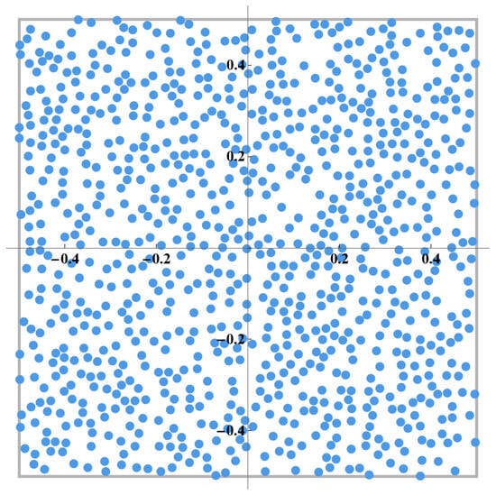
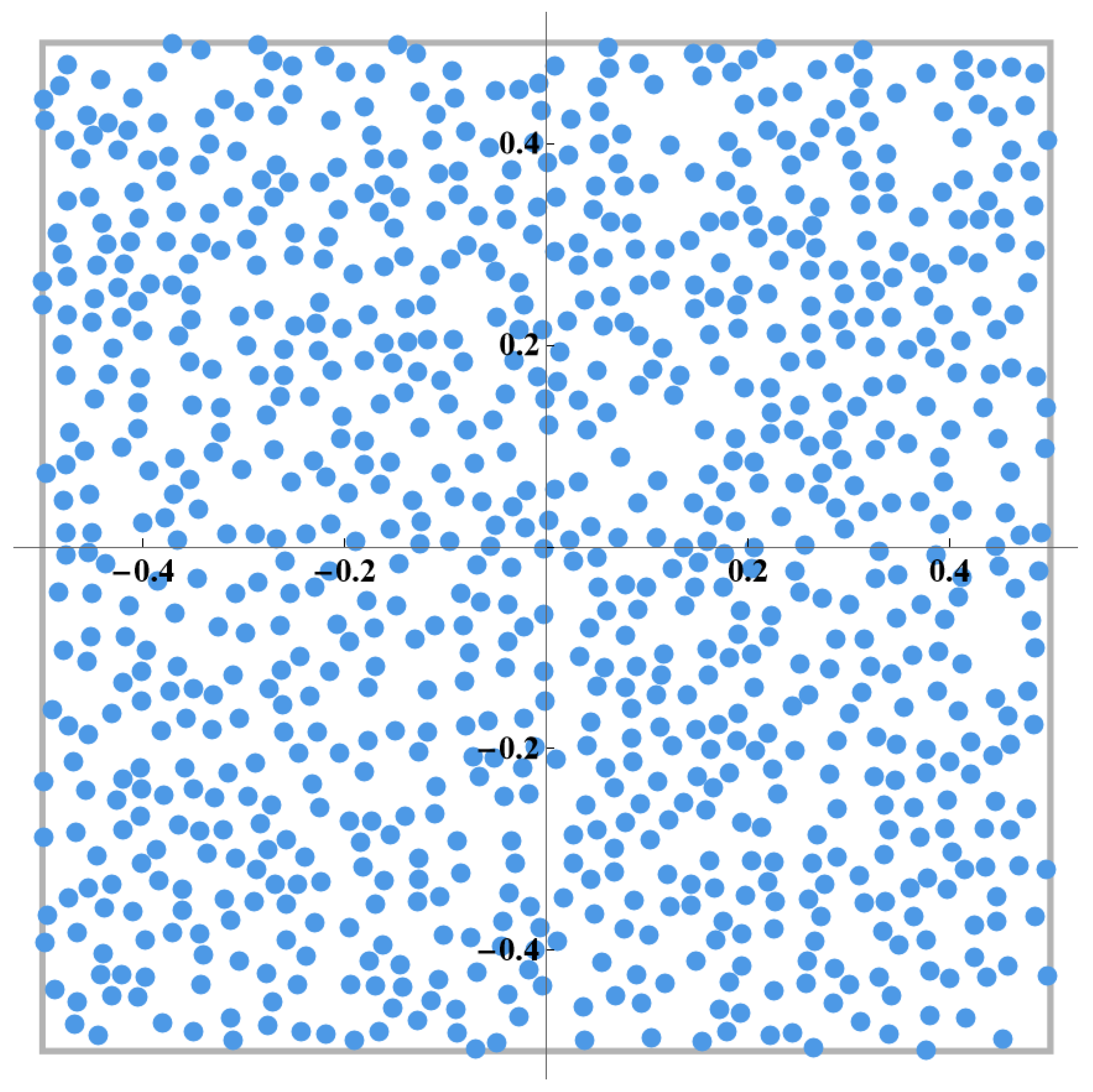
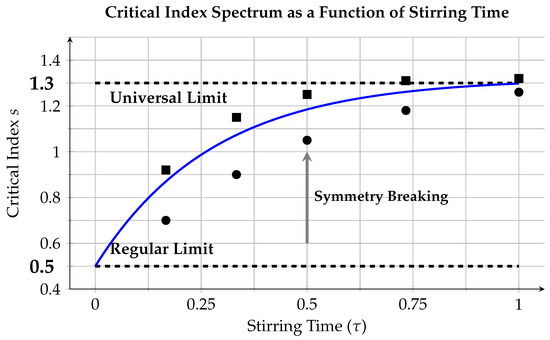
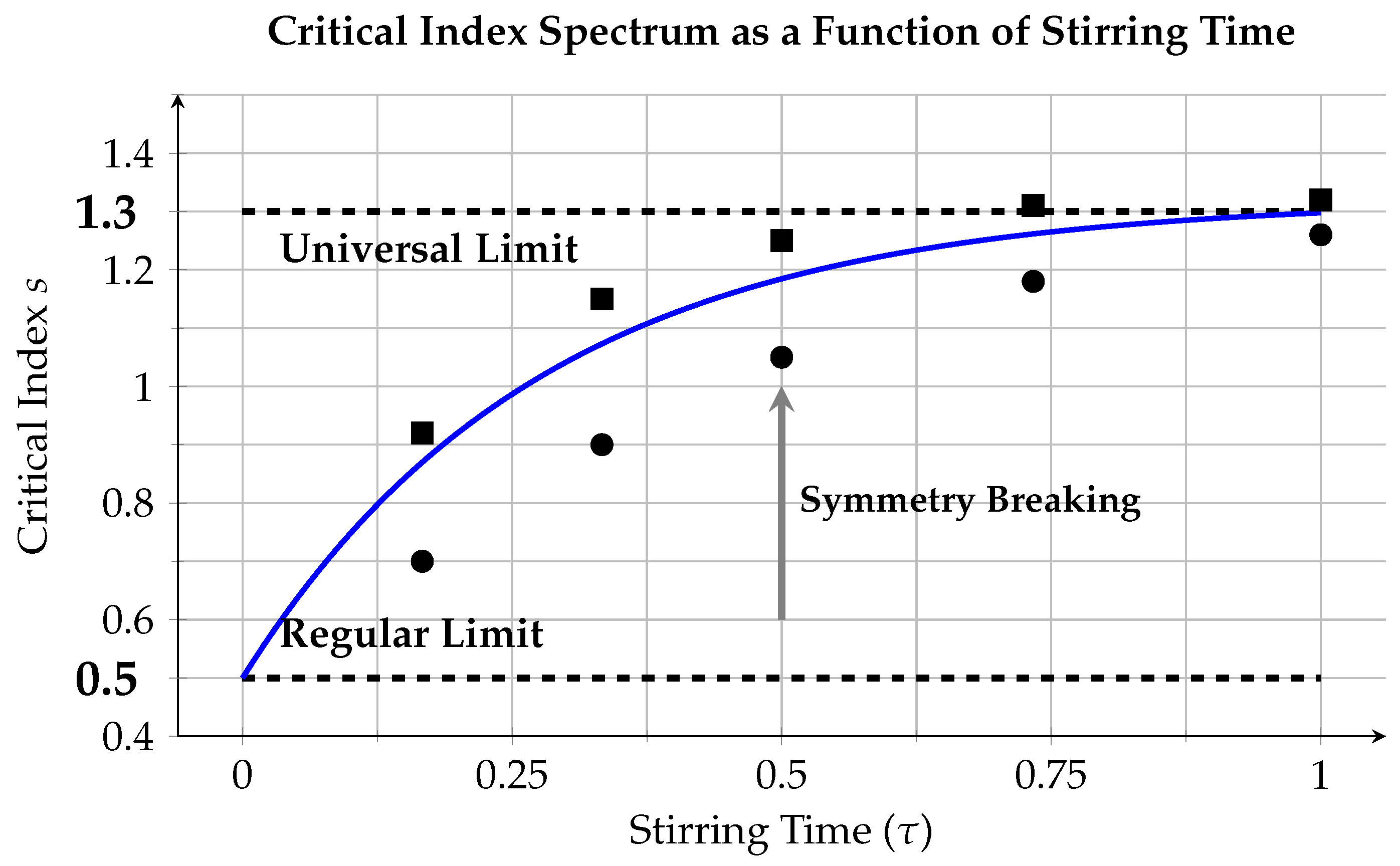
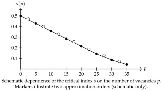
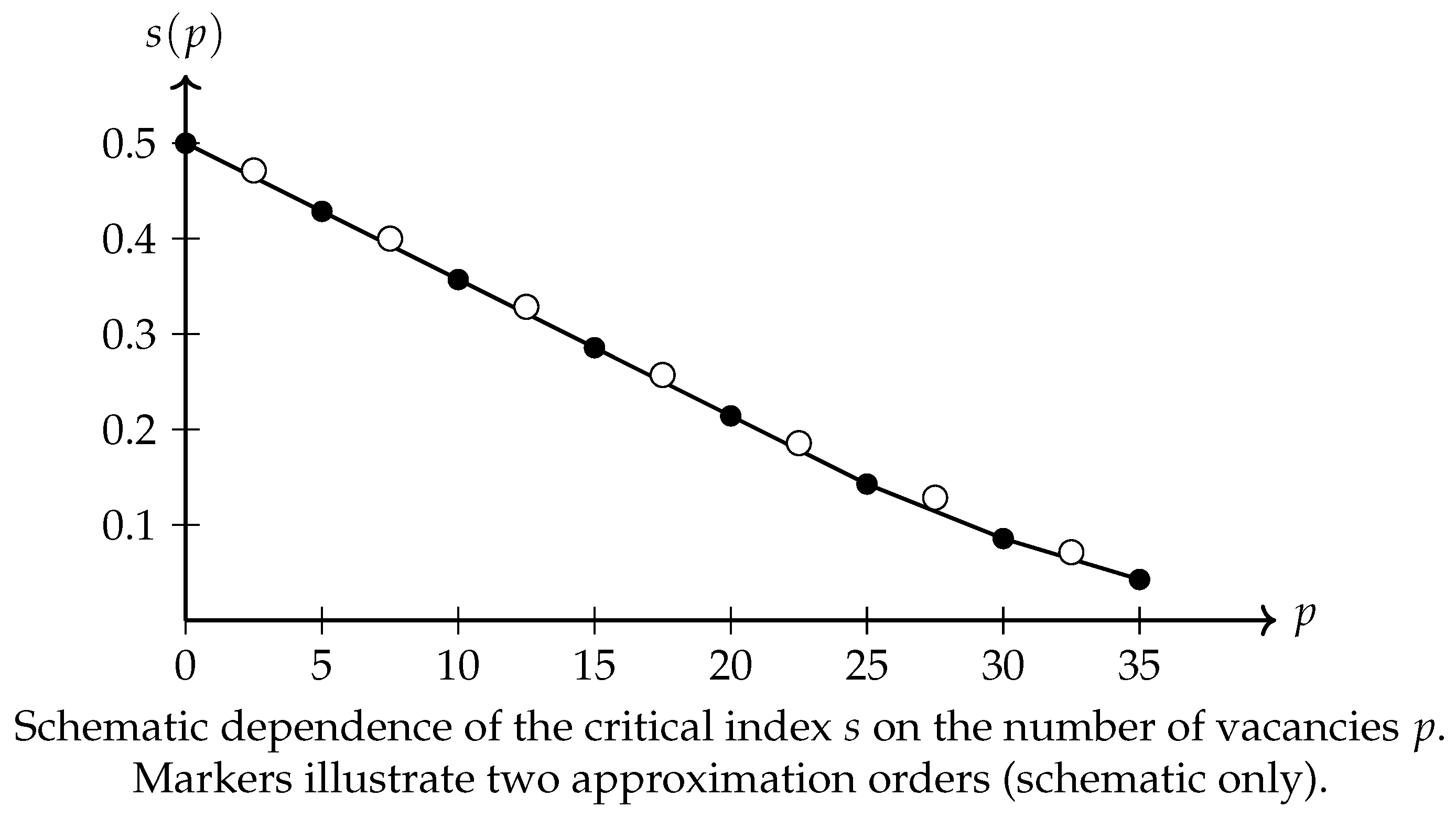
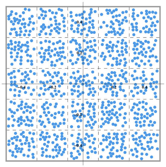
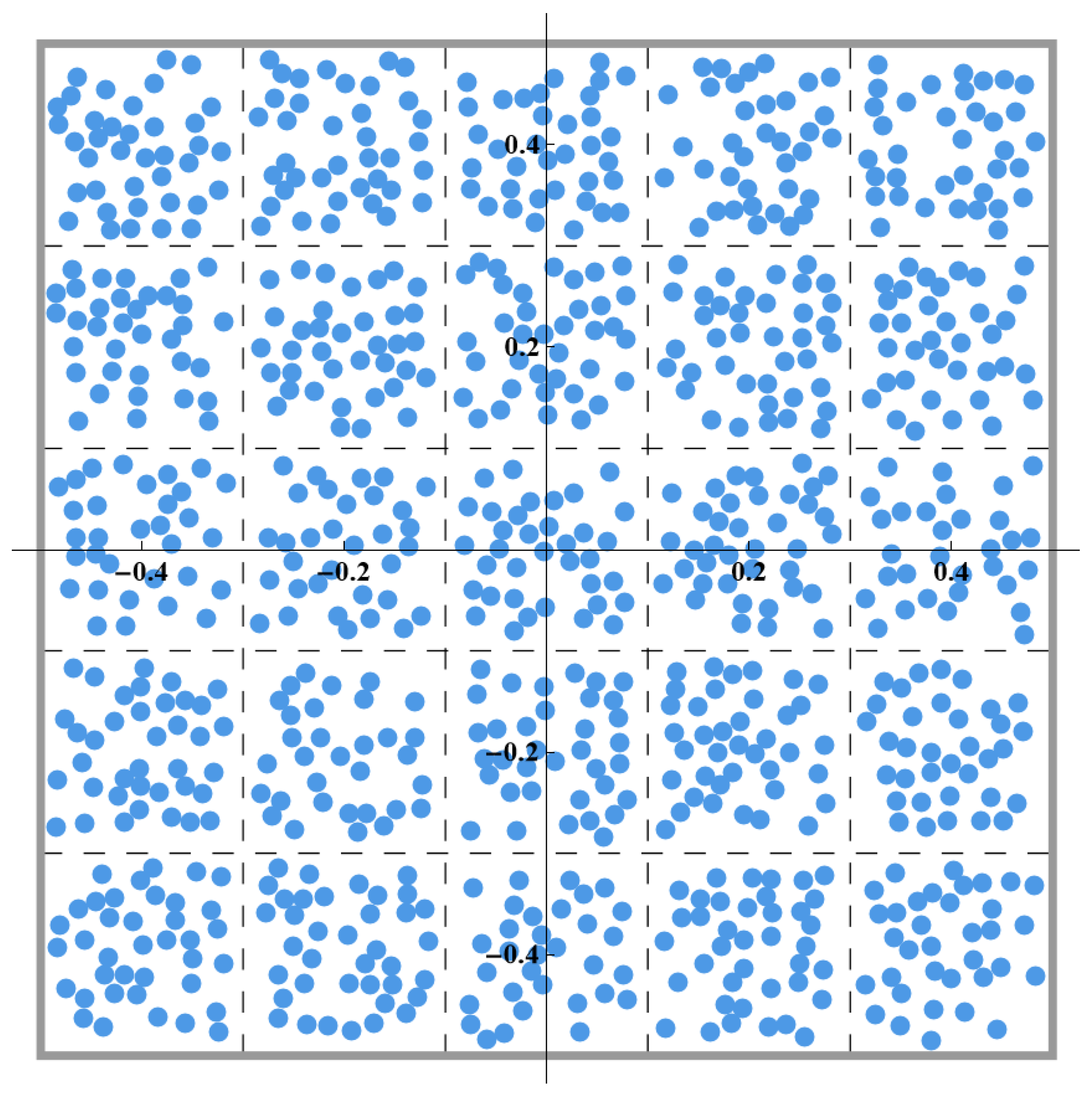

Disclaimer/Publisher’s Note: The statements, opinions and data contained in all publications are solely those of the individual author(s) and contributor(s) and not of MDPI and/or the editor(s). MDPI and/or the editor(s) disclaim responsibility for any injury to people or property resulting from any ideas, methods, instructions or products referred to in the content. |
© 2026 by the authors. Licensee MDPI, Basel, Switzerland. This article is an open access article distributed under the terms and conditions of the Creative Commons Attribution (CC BY) license.