Unit Linear Failure Rate Distribution with Applications in Socioeconomic and Reliability Data

Abstract

In this paper, a new probability model is suggested, known as the Unit Linear Failure Rate Distribution (ULFRD), which is used to analyse data expressed on a unit interval (0, 1), e.g., proportions, rates, and normalised indices. The proposed model is a transformation of the classical linear failure rate distribution to finite domains and gives us the opportunity to have shapes with a variety of shapes that can model any hazard rate behaviour, such as bathtub-shaped ones that are common in reliability research. Various fundamental statistical features of the distribution are obtained. The parameter estimation is analysed under Type-II censoring, where maximum likelihood and Bayesian estimations are used. Bayesian estimates are obtained under a symmetric and an asymmetric loss of a Metropolis–Hastings within a Gibbs approximation. The analyses of the estimates’ performance are performed via a simulation study of various sample sizes and censoring plans. Lastly, the generalisability of the proposed model is also demonstrated with two real datasets in the socioeconomic and reliability settings. The findings prove that the ULFRD offers a flexible and competitive alternative to model-bound data.

1. Introduction

There are numerous real-world datasets, consisting of proportions, percentages, or rates, which are conveniently valued in the unit interval (0, 1). They include examples such as food insecurity indicators, reliability indices, financial ratios, environmental indicators, and biomedical measurements. Classical lifetime distributions that are formulated on $\left(0,\infty \right)$ are not suitable for modelling such bounded data.

A number of probability models, which are defined on the unit interval, are therefore available in the literature. Such commonly used models include the beta and Kumaraswamy distributions, but more recent models involve the unit Weibull and unit Lindley distributions. These models have performed well in a number of areas, and some of the areas of application include reliability analysis, economics, and environmental studies; for more details, see Sapkota et al. [1] and Abd El-Bar et al. [2]. Nonetheless, a few distributions can cover all potential shapes of bounded data, prompting ongoing work on new flexible unit distributions that can accommodate various skewness shapes and hazard rate behaviours. Based on this concept, we propose a new unit distribution derived from the transformation of the linear failure rate distribution. The resulting model is known as the ULFRD and offers a flexible model of data that is bounded. Unit distributions provide realistic and interpretable models by guaranteeing that modelled values do not exceed the limits of validity and that distributional shapes are flexible. Consequently, they find wide applications in applied statistics, reliability analysis, and Bayesian studies.

On the other hand, more recent literature has discussed Bayesian inference of extended lifetime models and generalised distributions; some examples are Akhtar et al. [3], Akhtar and Alharthi [4], and Mehdi et al. [5]. These contributions point to the increased interest in flexible statistical models of reliability and lifetime analysis. Nevertheless, the majority of existing models are specified on the positive real line, so the current study develops a unit distribution of limited data on the interval (0, 1).

Extensive research has been devoted to the construction of unit distributions to describe bounded phenomena occurring in various fields of application. Initial work in this area was carried out by Mazucheli et al. [6], who defined the unit-Weibull distribution and discussed its inferential properties, and Mazucheli et al. [7], who defined the unit-Gompertz distribution to model growth processes. Ghitany et al. [8] later provided the unit-inverse Gaussian distribution as an alternative distribution to classical two-parameter distributions that are defined on the unit interval. Günduz et al. [9] constructed a family of unit distributions on the basis of the Johnson rule, thus increasing the modelling flexibility of bounded data, while Ribeiro-Reis [10] presented a unit log-logistic regression model.

Recent years have witnessed a growing focus on creating more flexible unit models with better inferential behaviour and increased applicability. Haque et al. [11] stated the unit-modified Burr-III distribution, meaning that the parameters can be estimated and the model can be proven, but Bakouch et al. [12] presented the two-parameter unit-exponential distribution, which can be applied in environmental and engineering applications. More recently, the unit two-parameter Mirra distribution was analysed in more detail by Al-Omari et al. [13], who focused on the reliability analysis, the procedure of estimating the distribution, and its practical implementation. Bui et al. [14] suggested a modified linear failure rate distribution that is able to take the bathtub-shaped hazard functions in the larger reliability frame. Moreover, Korkmaz and Korkmaz [15] presented the unit log-log distribution and discussed its statistical characteristics and quantile regression modelling, especially in the educational measurement analysis. Lastly, Sarhan et al. [16] and Sarhan and Sobh [17] suggested the unit-modified Weibull and the unit-exponentiated Weibull distributions, respectively. This proposal continues to testify to the persistence of methodological growth and increasing popularity of unit distribution theory.

This paper proposes a new distribution defined on the unit interval, referred to as the ULFRD, and investigates its main statistical and reliability properties. Reliability analysis and failure rate modelling are essential in modern engineering, as accurate system prediction affects performance, safety, and cost efficiency.

The Linear Failure Rate Distribution (LFRD), introduced by Barlow and Proschan [18], is a versatile model that can be used to study failure behaviour that depends on time and is a popular method of reliability analysis.

Let X follow LFRD with a cumulative distribution function (CDF),

$$F_X\left(x\right)=P(X\le x)=1-\exp \left\{-\alpha x-{\displaystyle \frac{\beta }{2}}{x}^2\right\},x>0,\alpha >0,\beta >0.$$

(1)

By applying the following transform,

$$Y=e^{-X}\to X=-lnY,0<y<1,$$

the ULFRD can be derived as will be illustrated in Section 2. The rest of this paper is organised as follows: Section 2 provides a description of the ULFRD. Section 3 presents statistical properties of the ULFRD, including the moment-generating function, rth moments, the characteristic function, order statistics and Rényi entropy. Section 4 presents the maximum likelihood estimation (MLE) based on Type-II censoring and the information matrix used to estimate the unknown parameters under consideration, as well as the confidence intervals for each parameter. Section 4 also deals with Bayesian estimation under the symmetric and asymmetric loss functions computed using the Markov Chain Monte Carlo (MCMC) technique. The simulation and a real-life dataset are presented in Section 5. The conclusion is reported in Section 6.

2. Unit Linear Failure Rate Distribution

The ULFRD is a bounded lifetime distribution defined on the unit interval (0, 1). It is obtained by transforming the LFRD to the unit interval and is widely used in reliability theory, survival analysis, and modelling proportions or rates. The CDF of the ULFRD is derived as follows:

$$\begin{array}{cc}\hfill G\left(y\right)& =P(Y\le y)=P(e^{-X}\le y)=P(\ln e^{-X}\le \ln y)\hfill \\ \hfill & =P(-X\le \ln y)=P(X\ge -\ln y)\hfill \\ \hfill & =1-P(X\le -\ln y)=1-F_X(-\ln y).\hfill \end{array}$$

By substituting $F_X\left(x\right)$,

$$\begin{array}{cc}\hfill G\left(y\right)& =1-\left[1-\exp \left\{-\alpha (-\ln y)-{\displaystyle \frac{\beta }{2}}{(-\ln y)}^2\right\}\right].\hfill \end{array}$$

By simplification,

$$\begin{array}{c}\hfill G\left(y\right)=y^{\alpha }\exp \left[-{\displaystyle \frac{\beta }{2}}{\left(\ln y\right)}^2\right],0<y<1.\end{array}$$

(2)

Differentiating $G\left(y\right)$ with respect to y, we obtain the probability density function (PDF) as follows:

$$\begin{array}{c}\hfill g\left(y\right)=\left({\displaystyle \frac{\alpha }{y}}-{\displaystyle \frac{\beta }{y}}\ln y\right)\exp \left\{\alpha \ln y-{\displaystyle \frac{\beta }{2}}{\left(\ln y\right)}^2\right\},0<y<1.\end{array}$$

By simplification,

$$\begin{array}{c}\hfill g\left(y\right)=(\alpha -\beta \ln y)y^{\alpha -1}\exp \left[-{\displaystyle \frac{\beta }{2}}{\left(\ln y\right)}^2\right],0<y<1.\end{array}$$

(3)

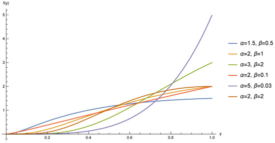
The density function in Equation (3) is structurally behavioural, which can be described analytically by its first derivative and boundary limits. As $y\to 0^{+}$, the exponential term involving ${\left(\log y\right)}^2$ dominates and forces $g\left(y\right)\to 0$, ensuring that the density does not diverge at the lower boundary. As $y\to 1^{-}$, since $\log y\to 0$, the density converges to $\alpha$, implying finite and parameter-controlled behaviour near the upper boundary. In order to further demonstrate the flexibility of the ULFRD, the density function was plotted, as shown in Figure 1, as a parameter with various combinations $(\alpha ,\beta )$. The parameter values chosen prove that the distribution may take various shapes based on the parameters’ interactions. Specifically, the density can be observed to be growing or unimodal, which results from the influence of the power component mediated by the value of alpha and the log-quadratic curvature mediated by the value of beta. These visual examples are coupled with the analytical discussion above and establish that the ULFRD can fit a selection of distributional shapes on the unit interval.

Figure 1. PDF of the ULFRD.

The monotonicity and possible unimodality of the density are governed by the sign of its first derivative $g^{\prime }\left(y\right)$, which depends explicitly on the interaction between $\alpha$ and $\beta$. Different parameter combinations may therefore produce increasing or unimodal shapes, as observed in the graphical illustrations.

The hazard rate function,

$$h\left(y\right)={\displaystyle \frac{g\left(y\right)}{1-G\left(y\right)}},$$

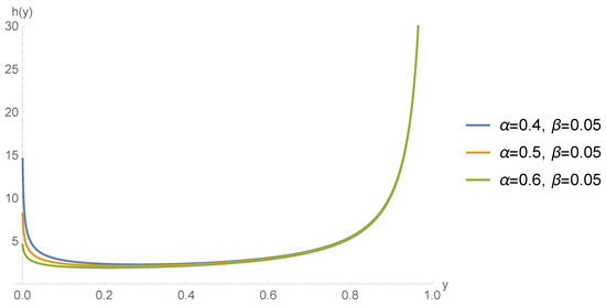
inherits its structural flexibility from the nonlinear dependence of both $g\left(y\right)$ and $G\left(y\right)$ on the parameters. Since the sign of the derivative $h^{\prime }\left(y\right)$ determines whether the hazard is increasing, decreasing, or non-monotone, and because $h^{\prime }\left(y\right)$ involves both $g^{\prime }\left(y\right)$ and $g\left(y\right)$, the interaction between $\alpha$ (power effect) and $\beta$ is conservative. The log-quadratic curvature effect allows multiple hazard regimes. The ULFR model, therefore, allows admitting the growth of and possibly non-monotone hazard behaviours due to changes in parameter values. The variety of forms shown in Figure 1 is thus a direct result of the derivative form of the model as opposed to a graphical representation.

The hazard rate function can be derived as follows:

$$\begin{array}{c}\hfill h\left(y\right)={\displaystyle \frac{\beta \ln \left(y\right)-\alpha }{y-y^{(1-\alpha )}{e}^{\frac{1}{2}\beta {\ln }^2\left(y\right)}}}\end{array}$$

(4)

Besides determining the bathtub-shaped behaviour through the sign of the first derivative of the hazard function, curvature-based useful life period analysis may also be conducted. In accordance with the conventional geometrical reasoning, the curvature function will be

$$\kappa \left(t\right)={\displaystyle \frac{\left|h^{″}\left(t\right)\right|}{{\left(1+{\left(h^{\prime }\left(t\right)\right)}^2\right)}^{3/2}}}$$

and it can be scrutinised to define the time interval between its local extrema, which defines the stage of fairly constant useful life of the hazard curve. This type of analysis is specific to the parameters and can be performed numerically to be implemented in real-life applications; for more details, see Choudhary et al. [19].

To conclude, the ULFRD is a versatile and general modelling structure that can effectively model a large variety of hazard rate behaviours, as shown in Figure 2. Its density and hazard functions exhibit systematic behaviour in response to a change in model parameters, and this is shown in Figure 1 and Figure 2. The flexibility of the distribution renders it especially appropriate to the analysis of survival data, notably in any program or field that uses censored observations.

Figure 2. Hazard rate function of the ULFRD.

3. Statistical Properties for ULFRD

This section draws various basic statistical characteristics of the ULFRD. Such properties are the moment-generating function, moments, characteristic function, order statistics, and Rényi entropy. The results of the obtained analysis provide a more profound understanding of the distributional structure and behaviour of the ULFRD.

3.1. Moment-Generating Function

The moment-generating function of Y is defined as

$$\begin{array}{c}\hfill M_Y\left(t\right)=E\left(e^{tY}\right)={\int }_0^1{e}^{ty}g\left(y\right)dy.\end{array}$$

(5)

Using the series expansion

$$\begin{array}{c}\hfill e^{tY}=\sum _{k=0}^{\infty }{\displaystyle \frac{t^k{y}^k}{k!}},\end{array}$$

(6)

by applying (4) in (3), we obtain

$$M_Y\left(t\right)=\sum _{k=0}^{\infty }{\displaystyle \frac{t^k}{k!}}{\int }_0^1{y}^{k+\alpha -1}(\alpha -\beta \ln y)\exp \left[-{\displaystyle \frac{\beta }{2}}{\left(\ln y\right)}^2\right]dy.$$

Let

$$u=\ln y,y=e^u,dy=e^{u}du,-\infty <u<0.$$

Then,

$$M_Y\left(t\right)=\sum _{k=0}^{\infty }{\displaystyle \frac{t^k}{k!}}{\int }_{-\infty }^0{e}^{(k+\alpha )u}(\alpha -\beta u)\exp \left[-{\displaystyle \frac{\beta }{2}}{u}^2\right]du.$$

By completing the Square, we write

$$-{\displaystyle \frac{\beta }{2}}{u}^2+(k+\alpha )u=-{\displaystyle \frac{\beta }{2}}{\left(u-{\displaystyle \frac{k+\alpha }{\beta }}\right)}^2+{\displaystyle \frac{{(k+\alpha )}^2}{2\beta }}.$$

Hence,

$$M_Y\left(t\right)=\sum _{k=0}^{\infty }{\displaystyle \frac{t^k}{k!}}\exp \left[{\displaystyle \frac{{(k+\alpha )}^2}{2\beta }}\right]{\int }_{-\infty }^0(\alpha -\beta u)\exp \left[-{\displaystyle \frac{\beta }{2}}{\left(u-{\displaystyle \frac{k+\alpha }{\beta }}\right)}^2\right]du.$$

From Gaussian standardisation, Let

$$z=\sqrt{{\displaystyle \frac{\beta }{2}}}\left(u-{\displaystyle \frac{k+\alpha }{\beta }}\right),dz=\sqrt{{\displaystyle \frac{\beta }{2}}}du.$$

Under this transformation, the integral involved in the derivation reduces to standard Gaussian integrals expressed in terms of the complementary error function $\mathrm{erfc}(·)$ (see Gradshteyn and Ryzhik [20]). Recall that the complementary error function is defined by

$$\mathrm{erfc}\left(a\right)={\displaystyle \frac{2}{\sqrt{\pi }}}{\int }_a^{\infty }{e}^{-t^2}dt,$$

which implies

$${\int }_a^{\infty }{e}^{-t^2}dt={\displaystyle \frac{\sqrt{\pi }}{2}}\mathrm{erfc}\left(a\right).$$

Moreover, using the well-known identity

$${\int }_{-\infty }^{\infty }{e}^{-x^2}dx=\sqrt{\pi },$$

it follows that

$${\int }_{-\infty }^a{e}^{-x^2}dx={\int }_{-\infty }^{\infty }{e}^{-x^2}dx-{\int }_a^{\infty }{e}^{-t^2}dt={\displaystyle \frac{\sqrt{\pi }}{2}}\mathrm{erfc}(-a).$$

By combining the above results and simplifying the resulting expression, the moment-generating function of the ULFRD is finally obtained as

$$\begin{array}{c}\hfill M_Y\left(t\right)=\sum _{k=0}^{\infty }{\displaystyle \frac{t^k}{k!}}\left[1-{\displaystyle \frac{k\sqrt{\pi }}{\sqrt{2\beta }}}\exp \left({\displaystyle \frac{{(k+\alpha )}^2}{2\beta }}\right)\mathrm{erfc}\left({\displaystyle \frac{k+\alpha }{\sqrt{2\beta }}}\right)\right].\end{array}$$

(7)

3.2. The rth Moment

The rth moment is

$$E\left(Y^r\right)={\int }_0^1{y}^{r+\alpha -1}(\alpha -\beta \ln y)\exp \left[-{\displaystyle \frac{\beta }{2}}{\left(\ln y\right)}^2\right]dy.$$

By transformation, let

$$u=\ln y,y=e^u,dy=e^{u}du,-\infty <u<0.$$

Then, the above expression reduces to

$$E\left(Y^r\right)={\int }_{-\infty }^0(\alpha -\beta u)\exp \left[-{\displaystyle \frac{\beta }{2}}{u}^2+(r+\alpha )u\right]du.$$

By completing the square,

$$-{\displaystyle \frac{\beta }{2}}{u}^2+(r+\alpha )u=-{\displaystyle \frac{\beta }{2}}{\left(u-{\displaystyle \frac{r+\alpha }{\beta }}\right)}^2+{\displaystyle \frac{{(r+\alpha )}^2}{2\beta }}.$$

Consequently,

$$E\left(Y^r\right)=exp\left[{\displaystyle \frac{{(r+\alpha )}^2}{2\beta }}\right]{\int }_{-\infty }^0(\alpha -\beta u)\exp \left[-{\displaystyle \frac{\beta }{2}}{\left(u-{\displaystyle \frac{r+\alpha }{\beta }}\right)}^2\right]du.$$

Applying Gaussian standardisation, let

$$z=\sqrt{{\displaystyle \frac{\beta }{2}}}\left(u-{\displaystyle \frac{r+\alpha }{\beta }}\right),du=\sqrt{{\displaystyle \frac{2}{\beta }}}dz.$$

Then,

$$E\left(Y^r\right)=\sqrt{{\displaystyle \frac{2}{\beta }}}\exp \left[{\displaystyle \frac{{(r+\alpha )}^2}{2\beta }}\right]{\int }_{-\infty }^{-{\displaystyle \frac{r+\alpha }{\sqrt{2\beta }}}}\left(-\sqrt{2\beta }z-r\right)e^{-z^2}dz.$$

Then, the integral can be expressed in terms of the complementary error function. By splitting the integral and using standard error-function identities, the rth moment is finally obtained as

$$\begin{array}{c}\hfill E\left(Y^r\right)=1-r\sqrt{{\displaystyle \frac{\pi }{2\beta }}}\exp \left({\displaystyle \frac{{(r+\alpha )}^2}{2\beta }}\right)\mathrm{erfc}\left({\displaystyle \frac{r+\alpha }{\sqrt{2\beta }}}\right).\end{array}$$

(8)

3.3. Characteristic Function

The characteristic function exists for any probability distribution, in contrast to the moment-generating function, which may not exist for all distributions. The characteristic function of Y is defined as

$${\varphi }_Y\left(t\right)=E\left(e^{itY}\right),i=\sqrt{-1},t\in \mathbb{R}.$$

Using the power series expansion,

$${\varphi }_Y\left(t\right)=\sum _{k=0}^{\infty }{\displaystyle \frac{{\left(it\right)}^k}{k!}}E\left(Y^k\right).$$

Substituting the corresponding moment expression yields the explicit form of the characteristic function.

$$\begin{array}{c}\hfill {\varphi }_Y\left(t\right)=\sum _{k=0}^{\infty }{\displaystyle \frac{{\left(it\right)}^k}{k!}}\left[1-k\sqrt{{\displaystyle \frac{\pi }{2\beta }}}\exp \left(-{\displaystyle \frac{{(k+\alpha )}^2}{2\beta }}\right)\mathrm{erfc}\left({\displaystyle \frac{k+\alpha }{\sqrt{2\beta }}}\right)\right].\end{array}$$

(9)

3.4. Order Statistics

Order statistics are fundamental tools in probability and statistics, as they describe the behaviour of ordered sample values and have wide applications in statistics, reliability theory, quality control, risk analysis and engineering. Let $Y_1,Y_2,\dots ,Y_n$ be an i.i.d. sample from the Unit Linear Failure Rate distribution, and denote the order statistics by

$$Y_{\left(1\right)}\le Y_{\left(2\right)}\le \cdots \le Y_{\left(n\right)}.$$

The PDF of the kth order statistic is given by

$$f_{Y_{\left(k\right)}}\left(y\right)={\displaystyle \frac{n!}{(k-1)!(n-k)!}}{\left[G\left(y\right)\right]}^{k-1}{[1-G\left(y\right)]}^{n-k}g\left(y\right),$$

where $G\left(y\right)$ and $g\left(y\right)$ are the CDF and PDF of the ULFRD, respectively.

Replacing $g\left(y\right)$ and $G\left(y\right)$, we obtain the PDF of the kth order statistic of ULFRD, as below:

$$\begin{array}{c}\hfill f_{Y_{\left(k\right)}}\left(y\right)={\displaystyle \frac{n!}{(k-1)!(n-k)!}}(\alpha -\beta \ln y)y^{\alpha k-1}{e}^{-{\displaystyle \frac{\beta k}{2}}{\left(\ln y\right)}^2}{\left[1-y^{\alpha }{e}^{-{\displaystyle \frac{\beta }{2}}{\left(\ln y\right)}^2}\right]}^{n-k}.\end{array}$$

(10)

Special Cases

Minimum ($k=1$):

$$f_{Y_{\left(1\right)}}\left(y\right)=n(\alpha -\beta \ln y)y^{\alpha -1}{e}^{-{\displaystyle \frac{\beta }{2}}{\left(\ln y\right)}^2}{\left[1-y^{\alpha }{e}^{-{\displaystyle \frac{\beta }{2}}{\left(\ln y\right)}^2}\right]}^{n-1}.$$

Maximum ($k=n$):

$$f_{Y_{\left(n\right)}}\left(y\right)=n(\alpha -\beta \ln y)y^{\alpha n-1}{e}^{-{\displaystyle \frac{n\beta }{2}}{\left(\ln y\right)}^2}.$$

3.5. Rényi Entropy

Rényi entropy is a generalised measure of uncertainty in probability theory and information theory. It extends Shannon entropy by introducing a parameter that controls the sensitivity to events with different probabilities.

The Rényi entropy is described as follows: for $\lambda >0$, $\lambda \ne 1$,

$$\begin{array}{c}\hfill H_{\lambda }\left(Y\right)={\displaystyle \frac{1}{1-\lambda }}\log \left({\int }_0^1{\left[g\left(y\right)\right]}^{\lambda }dy\right)={\displaystyle \frac{1}{1-\lambda }}\log \left(I\right),\end{array}$$

(11)

where

$$\begin{array}{c}\hfill I={\int }_0^1{\left[g\left(y\right)\right]}^{\lambda }dy.\end{array}$$

(12)

For the considered distribution, we have

$${\left[g\left(y\right)\right]}^{\lambda }=y^{\lambda (\alpha -1)}{(\alpha -\beta \ln y)}^{\lambda }\exp \left[-{\displaystyle \frac{\beta \lambda }{2}}{\left(\ln y\right)}^2\right].$$

Applying the transformation $u=\ln y$, the integral becomes

$$\begin{array}{c}\hfill I={\int }_{-\infty }^0{(\alpha -\beta u)}^{\lambda }\exp \left[-{\displaystyle \frac{\beta \lambda }{2}}{u}^2+(\lambda \alpha -\lambda +1)u\right]du.\end{array}$$

(13)

Completing the square yields the following:

$$-{\displaystyle \frac{\beta \lambda }{2}}[u^2-{\displaystyle \frac{2}{\beta \lambda }}(\alpha \lambda -\lambda +1)u]=-{\displaystyle \frac{\beta \lambda }{2}}{\left(u-{\displaystyle \frac{(\alpha \lambda -\lambda +1)}{\beta \lambda }}\right)}^2+{\displaystyle \frac{{(\alpha \lambda -\lambda +1)}^2}{2\beta \lambda }}.$$

Consequently,

$$\begin{array}{c}\hfill I=\exp \left[{\displaystyle \frac{{(\alpha \lambda -\lambda +1)}^2}{2\beta \lambda }}\right]{\int }_{-\infty }^0{(\alpha -\beta u)}^{\lambda }\exp \left[-{\displaystyle \frac{\beta \lambda }{2}}{\left(u-{\displaystyle \frac{\alpha \lambda -\lambda +1}{\beta \lambda }}\right)}^2\right]du.\end{array}$$

For simplifying, put

$$\begin{array}{c}\hfill \mu ={\displaystyle \frac{(\alpha \lambda -\lambda +1)}{\beta \lambda }}.\end{array}$$

Then, the integral become

$$\begin{array}{c}\hfill I=\exp \left[{\displaystyle \frac{{\mu }^2\beta \lambda }{2}}\right]{\int }_{-\infty }^0{(\alpha -\beta u)}^{\lambda }\exp \left[-{\displaystyle \frac{\beta \lambda }{2}}{(u-\mu )}^2\right]du.\end{array}$$

Thus, the final expression of the Rényi entropy $H_{\lambda }\left(Y\right)$ is

$$\begin{array}{c}\hfill H_{\lambda }\left(Y\right)={\displaystyle \frac{1}{1-\lambda }}\left[{\displaystyle \frac{{\mu }^2\beta \lambda }{2}}+\log {\int }_{-\infty }^0{(\alpha -\beta u)}^{\lambda }\exp \left[-{\displaystyle \frac{\beta \lambda }{2}}{(u-\mu )}^2\right]du\right].\end{array}$$

(14)

In summary, the important statistical characteristics of the ULFRD were obtained, providing analytical expressions on the nature of the probabilistic structure and distributional behaviour. Moreover, the expressions of derived moments can also be used to compute dispersion measures, the standard deviation and the variance, which can be obtained as direct derivations of moments obtained. These outcomes contribute to the theoretical insight into the ULFRD and its mathematical tractability to model data on the unit interval.

4. Parameter Estimation

This section outlines the estimation of the ULFR parameters with Type-II censoring by using both classical and Bayesian methods. The estimation is developed based on maximum likelihood, and the development of asymptotic confidence intervals is carried out based on the Fisher information matrix. The MCMC methods involving the Metropolis–Hastings algorithm are then used to perform Bayesian estimation to generate posterior estimates in both squared error and LINEX loss functions and their associated credible intervals.

4.1. Maximum Likelihood Estimation

MLE is one of the most widely used methods for estimating the parameters of continuous probability distributions due to its desirable statistical properties, including consistency, asymptotic unbiasedness, efficiency, and asymptotic normality. In this section, we derive the MLE parameters of the ULFRD and investigate their asymptotic properties.

Suppose that $y_{1:n}<y_{2:n}<\cdots <y_{r:n}$ is a Type-II censored sample of size r obtained from a life test on n items whose lifetimes have the ULFRD. The likelihood function of the observations $y_{1:n}<y_{2:n}<\cdots <y_{r:n}$ can be written in the following form:

$$\begin{array}{ccc}\hfill L\left(\alpha ,\beta ;y\right)& =& {\displaystyle \frac{n!}{(n-r)!}}\left[\prod _{i=1}^{r}g(y_{i:n},\alpha ,\beta )\right]{\left[1-G(y_{r:n},\alpha ,\beta )\right]}^{n-r}\hfill \\ & =& {\displaystyle \frac{n!}{(n-r)!}}\left[\prod _{i=1}^r{y}_{i:n}^{\alpha -1}(\alpha -\beta \ln y_{i:n})\exp \{-{\displaystyle \frac{\beta }{2}}{\left(\ln y_{i:n}\right)}^2\}\right]{[1-y_{r:n}^{\alpha }\exp \{-{\displaystyle \frac{\beta }{2}}{\left(\ln y_{r:n}\right)}^2\}]}^{n-r}.\hfill \end{array}$$

(15)

Then, the log-likelihood function $\mathsf{\ell }(\alpha ,\beta )$ can be written as

$$\mathsf{\ell }(\alpha ,\beta )\propto (\alpha -1)\sum _{i=1}^r\ln y_{i:n}+\sum _{i=1}^r\ln (\alpha -\beta \ln y_{i:n})-{\displaystyle \frac{\beta }{2}}\sum _{i=1}^r{\left(\ln y_{i:n}\right)}^2+(n-r)\ln [1-y_{r:n}^{\alpha }\exp \{-{\displaystyle \frac{\beta }{2}}{\left(\ln y_{r:n}\right)}^2\}].$$

(16)

Equating the partial derivatives of the log-likelihood function with respect to $\alpha$ and $\beta$, respectively, to zero gives

$${\displaystyle \frac{\mathsf{\partial }\mathsf{\ell }}{\mathsf{\partial }\alpha }}=\sum _{i=1}^r\ln y_{i:n}+\sum _{i=1}^r{\displaystyle \frac{1}{(\alpha -\beta \ln y_{i:n})}}-(n-r){\displaystyle \frac{y_{r:n}^{\alpha }\ln y_{r:n}\exp \{-\frac{\beta }{2}{\left(\ln y_{r:n}\right)}^2\}}{[1-y_{r:n}^{\alpha }\exp \{-\frac{\beta }{2}{\left(\ln y_{r:n}\right)}^2\}]}}=0,$$

(17)

and

$${\displaystyle \frac{\mathsf{\partial }\mathsf{\ell }}{\mathsf{\partial }\beta }}=-\sum _{i=1}^r{\displaystyle \frac{\ln y_{i:n}}{(\alpha -\beta \ln y_{i:n})}}+(n-r){\displaystyle \frac{\frac{1}{2}{\left(\ln y_{r:n}\right)}^2{y}_{r:n}^{\alpha }\ln y_{r:n}\exp \{-\frac{\beta }{2}{\left(\ln y_{r:n}\right)}^2\}}{[1-y_{r:n}^{\alpha }\exp \{-\frac{\beta }{2}{\left(\ln y_{r:n}\right)}^2\}]}}=0.$$

(18)

The resulting system consists of two nonlinear Equations (17) and (18) in the two unknown parameters $\alpha$ and $\beta$. Obtaining an exact closed-form solution for this system is analytically intractable. Consequently, the Newton–Raphson iterative method is used to obtain numerical approximations to the solutions of this nonlinear system. One can see that the ULFRD meets the usual regularity assumptions that are needed in the inference of likelihood. In the parameter space,

$$\theta =(\alpha ,\beta )\in \mathsf{\Theta }={(0,\infty )}^2,$$

where the parameter space $\mathsf{\Theta }$ is an open subset of ${\mathbb{R}}^2$, the log-likelihood is twice continuously differentiable with respect to the parameters, and the Fisher information, which is a square matrix, exists and is finite. In such a case, it can be seen that the asymptotic estimates are normally distributed, thus explaining the confidence intervals as provided in (19).

Confidence Intervals

The confidence interval (CI) for a population parameter $\theta$ is given by

$$P({\theta }_L\le \theta \le {\theta }_U)=1-\zeta ,$$

where ${\theta }_L$ and ${\theta }_U$ are the lower and upper confidence limits of the parameter $\theta$. For a large sample size, the population parameter $\theta$ has a normal distribution, i.e.,

$$P(-z_{{\displaystyle \frac{\zeta }{2}}}\le {\displaystyle \frac{\theta -\widehat{\theta }}{\sqrt{var\left(\theta \right)}}}\le z_{{\displaystyle \frac{\zeta }{2}}})=1-\zeta ,$$

Then, $\left(1-\zeta \right)100\%$ approximate confidence intervals (ACIs) for the parameters $\alpha$ and $\beta$ are of the form

$$\begin{array}{ccc}\hfill ({\widehat{\alpha }}_L,{\widehat{\alpha }}_U)& =& \widehat{\alpha }\pm z_{{\displaystyle \frac{\zeta }{2}}}\sqrt{var\left(\widehat{\alpha }\right)}\hfill \\ \hfill ({\widehat{\beta }}_L,{\widehat{\beta }}_U)& =& \widehat{\beta }\pm z_{{\displaystyle \frac{\zeta }{2}}}\sqrt{var\left(\widehat{\beta }\right)},\hfill \end{array}$$

(19)

where $z_{{\displaystyle \frac{\zeta }{2}}}$ is the value of the standard normal distribution leaving an area of ${\displaystyle \frac{\zeta }{2}}$ to the right, and $var\left(\widehat{\alpha }\right)$ and $var\left(\widehat{\beta }\right)$ represent asymptotic variances of MLEs of $\alpha$ and $\beta$, respectively. The asymptotic variances of the MLEs of $\alpha$ and $\beta$ can be evaluated from the inverse of the Fisher information matrix, which can be represented by the asymptotic covariance matrix as follows:

The asymptotic covariance matrix for the MLEs can be obtained by using the inverse of the asymptotic Fisher information matrix, as follows:

$$F^{-1}={\left[\begin{array}{cc}-{\displaystyle \frac{{\mathsf{\partial }}^2\mathsf{\ell }}{\mathsf{\partial }{\alpha }^2}}& -{\displaystyle \frac{{\mathsf{\partial }}^2\mathsf{\ell }}{\mathsf{\partial }\alpha \mathsf{\partial }\beta }}\\ -{\displaystyle \frac{{\mathsf{\partial }}^2\mathsf{\ell }}{\mathsf{\partial }\beta \mathsf{\partial }\alpha }}& -{\displaystyle \frac{{\mathsf{\partial }}^2\mathsf{\ell }}{\mathsf{\partial }{\beta }^2}}\end{array}\right]}_{\downarrow (\widehat{\alpha },\widehat{\beta })}^{-1}={\left[\begin{array}{cc}var\left(\widehat{\alpha }\right)& Cov(\widehat{\alpha },\widehat{\beta })\\ Cov(\widehat{\beta },\widehat{\alpha })& var\left(\widehat{\beta }\right)\end{array}\right]}_{\downarrow (\widehat{\alpha },\widehat{\beta })},$$

where the second partial derivatives of the log-likelihood function with respect to $\alpha$ and $\beta$, respectively, are obtained as

$${\displaystyle \frac{{\mathsf{\partial }}^2\mathsf{\ell }}{\mathsf{\partial }{\alpha }^2}}=-\sum _{i=1}^r{\displaystyle \frac{1}{{(\alpha -\beta \ln y_{i:n})}^2}}-(n-r){\displaystyle \frac{y_{r:n}^{\alpha }{\left(\ln y_{r:n}\right)}^2\exp \{-\frac{\beta }{2}{\left(\ln y_{r:n}\right)}^2\}}{{[1-y_{r:n}^{\alpha }\exp \{-\frac{\beta }{2}{\left(\ln y_{r:n}\right)}^2\}]}^2}},$$

$${\displaystyle \frac{{\mathsf{\partial }}^2\mathsf{\ell }}{\mathsf{\partial }\alpha \mathsf{\partial }\beta }}=\sum _{i=1}^r{\displaystyle \frac{\ln y_{i:n}}{{(\alpha -\beta \ln y_{i:n})}^2}}-{\displaystyle \frac{(n-r)}{2}}{\displaystyle \frac{y_{r:n}^{\alpha }{\left(\ln y_{r:n}\right)}^3\exp \{-\frac{\beta }{2}{\left(\ln y_{r:n}\right)}^2\}}{{[1-y_{r:n}^{\alpha }\exp \{-\frac{\beta }{2}{\left(\ln y_{r:n}\right)}^2\}]}^2}},$$

and

$${\displaystyle \frac{{\mathsf{\partial }}^2\mathsf{\ell }}{\mathsf{\partial }{\beta }^2}}=-\sum _{i=1}^r{\displaystyle \frac{{\left(\ln y_{i:n}\right)}^2}{{(\alpha -\beta \ln y_{i:n})}^2}}-{\displaystyle \frac{(n-r)}{4}}{\displaystyle \frac{y_{r:n}^{\alpha }{\left(\ln y_{r:n}\right)}^4\exp \{-\frac{\beta }{2}{\left(\ln y_{r:n}\right)}^2\}}{{[1-y_{r:n}^{\alpha }\exp \{-\frac{\beta }{2}{\left(\ln y_{r:n}\right)}^2\}]}^2}}.$$

4.2. Bayesian Estimation Using MCMC Technique

In this section, we obtain Bayesian estimates of the parameters of the ULFRD and their corresponding credible intervals. Suppose the prior knowledge about the parameters $\alpha$ and $\beta$ is represented by the independent informative Gamma priors as follows:

$$\begin{array}{c}\pi \left(\alpha \right)\propto {\alpha }^{a_1-1}{e}^{-\alpha b_1},\alpha >0,\\ \\ \pi \left(\beta \right)\propto {\beta }^{a_2-1}{e}^{-\beta b_2},\beta >0,\end{array}$$

where $a_1,a_2,b_1$ and $b_2$ are the hyperparameters, and they are non-negative. In most Bayesian models, the positive model parameters are almost given independent Gamma priors because they are convenient and flexible on the positive real line. In order to capture non-informative or diffuse prior knowledge, due to limited knowledge about the population parameters in practical situations, the hyperparameters are chosen to be small enough (e.g., $a_1$ = $a_2$ = $b_1$ = $b_2$ = $0.001$), resulting in a very dispersed prior with large variance and small prior information in the posterior model. In this restrictive regime, the Gamma prior is an approximation of a non-informative prior on the positive parameter space, which permits the likelihood function to prevail in the inference. As a result, the posterior estimates that are obtained are mostly representative of the observed data.

Then, the joint prior of the parameters $\alpha$ and $\beta$ can be written as

$$\pi \left(\alpha ,\beta \right)\propto {\alpha }^{a_1-1}{\beta }^{a_2-1}{e}^{-\alpha b_1-\beta b_2},\alpha >0,\beta >0.$$

(20)

The joint posterior density function of $\alpha$ and $\beta$, denoted by ${\pi }^{*}(\alpha ,\beta |\underline{y})$, can be written as

$${\pi }^{*}(\alpha ,\beta |\underline{y})={\displaystyle \frac{L\left(\alpha ,\beta \right)\times \pi \left(\alpha ,\beta \right)}{{\int }_0^{\infty }{\int }_0^{\infty }L\left(\alpha ,\beta \right)\times \pi \left(\alpha ,\beta \right)d\alpha d\beta }}.$$

(21)

By using Equations (15) and (20) to substitute in Equation (21), the joint posterior density function of $\alpha$ and $\beta$ is given by

$$\begin{array}{cc}\hfill {\pi }^{*}(\alpha ,\beta |\underline{y})& \propto {\alpha }^{a_1-1}{\beta }^{a_2-1}{e}^{-\alpha b_1-\beta b_2}\hfill \\ \hfill \times & \left[\prod _{i=1}^r{y}_{i:n}^{\alpha -1}(\alpha -\beta \ln y_{i:n})\exp \{-{\displaystyle \frac{\beta }{2}}{\left(\ln y_{i:n}\right)}^2\}\right]{[1-y_{r:n}^{\alpha }\exp \{-{\displaystyle \frac{\beta }{2}}{\left(\ln y_{r:n}\right)}^2\}]}^{n-r},\hfill \end{array}$$

(22)

where $K^{-1}$ is the normalising constant, equal to

$$\begin{array}{ccc}\hfill K^{-1}& =& {\int }_0^{\infty }{\int }_0^{\infty }{\alpha }^{a_1-1}{\beta }^{a_2-1}{e}^{-\alpha b_1-\beta b_2}\hfill \\ & & \times \left[\prod _{i=1}^r{y}_{i:n}^{\alpha -1}(\alpha -\beta \ln y_{i:n})\exp \{-{\displaystyle \frac{\beta }{2}}{\left(\ln y_{i:n}\right)}^2\}\right]{[1-y_{r:n}^{\alpha }\exp \{-{\displaystyle \frac{\beta }{2}}{\left(\ln y_{r:n}\right)}^2\}]}^{n-r}\hfill \end{array}$$

(23)

Therefore, the Bayes estimate of any function of the parameters $\alpha$ and $\beta$ such as $g(\alpha ,\beta )$ under a squared error loss function should be the posterior mean, i.e.,

$$g(\alpha ,\beta )={\displaystyle \frac{{\int }_0^{\infty }{\int }_0^{\infty }g(\alpha ,\beta )\times L\left(\alpha ,\beta \right)\times \pi \left(\alpha ,\beta \right)d\alpha d\beta }{{\int }_0^{\infty }{\int }_0^{\infty }g(\alpha ,\beta )\times L\left(\alpha ,\beta \right)\times \pi \left(\alpha ,\beta \right)d\alpha d\beta }}$$

(24)

The integrals given by Equation (24) cannot be obtained in explicit form, so the MCMC technique is applied to obtain an approximate value of these integrals, and then the Bayes estimates of the parameters $\alpha$ and $\beta$ is computed, also approximating the credible intervals. Then, the conditional posterior densities of $\alpha$ and $\beta$ can be given, respectively, as

$${\pi }_1^{*}\left(\alpha \right|\beta ,data)\propto {\alpha }^{a_1}{e}^{-\alpha b_1}\times \left[\prod _{i=1}^r{y}_{i:n}^{\alpha -1}\exp \{-{\displaystyle \frac{\beta }{2}}{\left(\ln y_{i:n}\right)}^2\}\right]{[1-y_{r:n}^{\alpha }\exp \{-{\displaystyle \frac{\beta }{2}}{\left(\ln y_{r:n}\right)}^2\}]}^{n-r},$$

(25)

and

$${\pi }_2^{*}\left(\beta \right|\alpha ,data)\propto {\beta }^{a_2}{e}^{-\beta b_2}\left[\prod _{i=1}^r(-\ln y_{i:n})\exp \{-{\displaystyle \frac{\beta }{2}}{\left(\ln y_{i:n}\right)}^2\}\right]{[1-y_{r:n}^{\alpha }\exp \{-{\displaystyle \frac{\beta }{2}}{\left(\ln y_{r:n}\right)}^2\}]}^{n-r}$$

(26)

The Metropolis algorithm was initially introduced by Metropolis et al. [21] and later generalised by Hastings [22] and is now known as the Metropolis–Hastings algorithm. It is an embedded method that generates samples of the posterior in the Gibbs sampling scheme, in accordance with the line of thinking of Tierney, as outlined in his book [23]. These backward pulls are then used to obtain the Bayes estimates of the parameters and the credible interval.

Specifically, after discarding the burn-in period, the Bayes estimates of the parameters under the squared error loss (SEL) function are obtained as the posterior means, given by

$$\begin{array}{c}{\alpha }_{MCMC}={\displaystyle \frac{1}{N-M}}\sum _{i=M+1}^N{\alpha }^{\left(i\right)},\\ \\ {\beta }_{MCMC}={\displaystyle \frac{1}{N-M}}\sum _{i=M+1}^N{\beta }^{\left(i\right)},\end{array}$$

In addition, the approximate Bayes estimate of parameters under the asymmetric LINEX (Linear Exponential) loss function is given as follows:

$$\begin{array}{ccc}\hfill {\widehat{\alpha }}_{Linex-Loss}& =& -{\displaystyle \frac{1}{c}}\log {\displaystyle \frac{1}{N-M}}\sum _{i=M+1}^N\left(\exp \left[-c{\alpha }^{\left(i\right)}\right]\right)\hfill \\ \hfill {\widehat{\beta }}_{Linex-Loss}& =& -{\displaystyle \frac{1}{c}}\log {\displaystyle \frac{1}{N-M}}\sum _{i=M+1}^N\left(\exp \left[-c{\beta }^{\left(i\right)}\right]\right),c\ne 0.\hfill \end{array}$$

(27)

The SEL function is widely used, which presumes equal penalties in case of errors in estimation. Nevertheless, overestimation and underestimation in a number of realistic scenarios might carry various implications. The LINEX (linear exponential) loss function is frequently used to consider such asymmetry. This loss function enables various penalties to be imposed on positive versus negative estimation errors, and it is mostly applicable in reliability and risk-based applications (see Varian [24]).

Moreover, the credible intervals (CRIs) for parameters are constructed using the empirical quantiles of the retained posterior samples; for more details, see Mahmoud et al. [25]. The posterior integrals have no closed-form solutions; thus, MCMC algorithms, namely the Metropolis–Hastings algorithm of Gibbs sampling, were employed to draw posterior samples. These samples were used to obtain Bayesian estimates using the squared error and LINEX loss functions as well as credible intervals.

Now, the following steps illustrate the process of the Metropolis–Hastings algorithm within Gibbs sampling:

(1)

Start with initial guess $\left({\alpha }^{\left(0\right)},{\beta }^{\left(0\right)}\right)$.

(2)

Set $j=1$.

(3)

Generate ${\alpha }^{\left(j\right)}$ and ${\beta }^{\left(j\right)}$ from ${\pi }_1^{*}\left({\alpha }^{(j-1)}\mid {\beta }^{(j-1)},\mathrm{data}\right)$ and ${\pi }_2^{*}\left({\beta }^{(j-1)}\mid {\alpha }^{\left(j\right)},\mathrm{data}\right)$ with the normal proposal distributions $N\left({\alpha }^{(j-1)},var\left(\alpha \right)\right)$ and $N\left({\beta }^{(j-1)},var\left(\alpha \right)\right)$.

(i)

Generate a proposal ${\alpha }^{*}$ from $N\left({\alpha }^{(j-1)},var\left(\alpha \right)\right)$ and ${\beta }^{*}$ from $N\left({\beta }^{(j-1)},var\left(\alpha \right)\right)$

(ii)

Evaluate the acceptance probabilities

$$\begin{array}{cc}\hfill {\eta }_{\alpha }& =\min \left[1,{\displaystyle \frac{{\pi }_1^{*}\left({\alpha }^{*}\mid {\beta }^{(j-1)},\mathrm{data}\right)}{{\pi }_1^{*}\left({\alpha }^{(j-1)}\mid {\beta }^{(j-1)},\mathrm{data}\right)}}\right],\hfill \\ \hfill {\eta }_{\beta }& =\min \left[1,{\displaystyle \frac{{\pi }_2^{*}\left({\beta }^{*}\mid {\alpha }^{\left(j\right)},\mathrm{data}\right)}{{\pi }_2^{*}\left({\beta }^{(j-1)}\mid {\alpha }^{\left(j\right)},\mathrm{data}\right)}}\right].\hfill \end{array}$$

(iii)

Generate a $u_1$ and $u_2$ from a Uniform $(0,1)$ distribution.

(iv)

If $u_1<{\eta }_{\alpha }$, accept the proposal and set ${\alpha }^{\left(j\right)}={\alpha }^{*}$; else, set ${\alpha }^{\left(j\right)}={\alpha }^{(j-1)}$.

(v)

If $u_2$$<{\eta }_{\beta }$, accept the proposal and set ${\beta }^{\left(j\right)}={\beta }^{*}$; else, set ${\beta }^{\left(j\right)}={\beta }^{(j-1)}$.

(4)

Set $j=j+1$.

(5)

Repeat Steps (3) and (4) N times and obtain ${\alpha }^{\left(i\right)}$ and ${\beta }^{\left(i\right)},i=1,2,...N$.

In order to guarantee the convergence and to remove the effect of the selection of initial values, the first M simulated varieties are discarded. Then, the selected samples are ${\alpha }^{\left(j\right)}$ and $,{\beta }^{\left(j\right)}$, $j=M+1,\dots ,N$, for sufficiently large N, forming approximate posterior samples that can be used to develop the Bayesian inferences.

5. Simulation and Data Analysis

This part describes a simulation study and uses real data to assess the performance of the proposed ULFRD and its practical applicability. The Monte Carlo simulation is carried out to examine the MLEs and Bayesian estimates when they are of different sample sizes and have different censoring rates, using their bias, mean squared error, interval lengths, and coverage probabilities. Besides this, two real-life datasets are also examined to illustrate the flexibility and goodness-of-fit of the model, thus showing the usefulness of the model in modelling bounded and censored data in real-world situations.

5.1. Simulation Study

Simulation studies are also significant in the evaluation and comparison of statistical inferences. A wide range of sample sizes was accounted for, in terms of n (30, 40, 50, and 60), as well as observed failures, r, and all calculations were completed with the help of Wolfram Mathematica, version 12. Samples from the ULFRD were generated through the uniform distribution by applying the inverse transformation method. The values of the parameters applied to create a simulated sample were considered to be $(\alpha ,\beta )=(0.05,0.03)$. Maximum likelihood and Bayesian estimation were used to estimate the parameters based on the symmetric SEL and the asymmetric LINEX loss functions. The MCMC method was used to compute the Bayesian estimates by applying the Metropolis–Hastings algorithm, with 2000 generated samples, and with the initial 600 samples being lost as burn-in. Comparison of the estimates was carried out based on the bias and mean squared error (MSE) measures obtained after 2000 replications. Besides that, the coverage probability (CP) and the average width (AW) of the associated confidence intervals were taken into account. Table 1, Table 2, Table 3 and Table 4 provide a summary of results.

Table 1. Bias and MSE values for $\alpha =0.05$.

		$\mathit{MLE}$		$\mathit{SEL}$		$\mathit{LINEX}$
n	r					$c=-2$		$c=2$
		Bias	MSE	Bias	MSE	Bias	MSE	Bias	MSE
30	15	$-0.0285$	$0.0068$	$-0.0092$	$0.0003$	$-0.0092$	$0.0003$	$-0.0093$	$0.0003$
30	20	$-0.0184$	$0.0035$	$-0.0116$	$0.0004$	$-0.0115$	$0.0003$	$-0.0117$	$0.0004$
40	20	$-0.0218$	$0.0047$	$-0.0070$	$0.0002$	$-0.0069$	$0.0002$	$-0.0070$	$0.0002$
50	30	$-0.0139$	$0.0023$	$-0.0065$	$0.0002$	$-0.0065$	$0.0002$	$-0.0065$	$0.0002$
60	50	$-0.0039$	$0.0001$	$-0.01051$	$0.0003$	$-0.0104$	$0.0003$	$-0.0106$	$0.0003$

Table 2. Bias and MSE values for $\beta =0.03$.

		$\mathit{MLE}$		$\mathit{SEL}$		$\mathit{LINEX}$
n	r					$c=-2$		$c=2$
		Bias	MSE	Bias	MSE	Bias	MSE	Bias	MSE
30	15	$0.0087$	$0.0005$	$-0.0053$	$0.0001$	$-0.0053$	$0.0001$	$-0.0053$	$0.0001$
30	20	$0.0065$	$0.0003$	$-0.0049$	$0.0001$	$-0.0049$	$0.0001$	$-0.0050$	$0.0001$
40	20	$0.0062$	$0.0003$	$-0.0052$	$0.0001$	$-0.0052$	$0.0001$	$-0.0052$	$0.0001$
50	30	$0.0046$	$0.0002$	$-0.0046$	$0.0001$	$-0.0046$	$0.0001$	$-0.0046$	$0.0001$
60	50	$0.0020$	$0.0001$	$-0.0033$	$0.0001$	$-0.0032$	$0.0001$	$-0.00321$	$0.0001$

Table 3. AWs and CPs for $\alpha =0.05$.

		$\mathit{ACI}$				$\mathit{CRI}$
n	r	$90\%$		$95\%$		$90\%$		$95\%$
		AW	CP	AW	CP	AW	CP	AW	CP
30	15	$0.2240$	$0.8940$	$0.2669$	$0.9520$	$0.0112$	$0.7700$	$0.0120$	$0.7900$
30	20	$0.1717$	$0.8860$	$0.2046$	$0.9375$	$0.0130$	$0.7445$	$0.0137$	$0.7595$
40	20	$0.1880$	$0.8820$	$0.2240$	$0.9460$	$0.0093$	$0.7820$	$0.0099$	$0.8000$
50	30	$0.1420$	$0.8900$	$0.1692$	$0.9405$	$0.0084$	$0.8025$	$0.0089$	$0.8165$
60	50	$0.0986$	$0.8765$	$0.1174$	$0.9340$	$0.0115$	$0.7805$	$0.0122$	$0.7940$

Table 4. AWs and CPs for $\beta =0.03$.

		$\mathit{ACI}$				$\mathit{CRI}$
n	r	$90\%$		$95\%$		$90\%$		$95\%$
		AW	CP	AW	CP	AW	CP	AW	CP
30	15	$0.0570$	$0.8955$	$0.0679$	$0.9485$	$0.0070$	$0.7660$	$0.0075$	$0.7880$
30	20	$0.0473$	$0.9050$	$0.0563$	$0.9580$	$0.0077$	$0.7540$	$0.0082$	$0.7710$
40	20	$0.0471$	$0.8915$	$0.0561$	$0.9405$	$0.0064$	$0.7795$	$0.0068$	$0.7970$
50	30	$0.0374$	$0.9005$	$0.0445$	$0.9475$	$0.0056$	$0.8020$	$0.0059$	$0.8165$
60	50	$0.0277$	$0.8950$	$0.0330$	$0.9445$	$0.0062$	$0.7880$	$0.0066$	$0.8005$

Table 1, Table 2, Table 3 and Table 4 present the summary of the simulation results according to 2000 replications of the results with various sample sizes and levels of censoring. Table 1 shows the bias and the mean squared error (MSE) of the estimators of alpha parameters. Both the bias and the MSE are found to reduce with the increase in the sample size n and the observed failures r, which means that the accuracy of the estimation increases with the increase in the sample size. The values of bias and MSE of the parameter beta are recorded in Table 2, and the same pattern is found in this case: the performance of the estimators increases with the availability of more information.

The average width (AW) and coverage probability (CP) of the interval estimates of alpha are shown in Table 3. The findings show that the interval widths reduce with the increase in sample size, and this shows greater accuracy of the estimators. The corresponding interval results of beta are reported in Table 4, where the same is observed. The approximate coverage probabilities of the confidence intervals are usually very similar to the nominal levels, whereas the Bayesian credible intervals are known to generate slightly lower coverage probabilities but are generally more stable under the simulated cases taken into account.

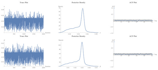
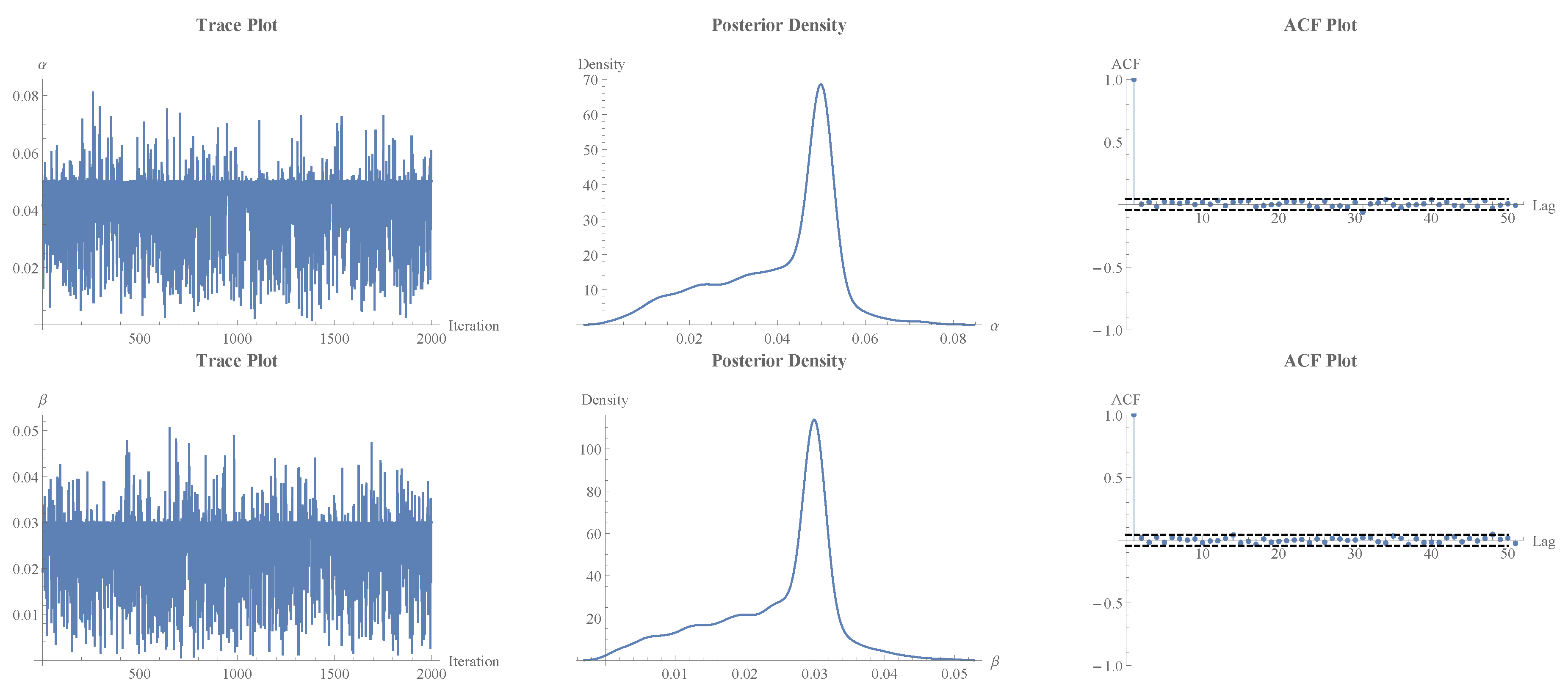
Using the MCMC, the diagnostic graphs of the parameters, $\alpha$ and $\beta$, the trace plot, the posterior density plot, and the autocorrelation functions (ACF) are represented in Figure 3. The trace plots reveal that the fluctuations are stable at constant levels, which means that the Markov chains are mixed well. As seen in the posterior density plots, the shape of the posterior distributions appears to be unimodal in nature. Further, the ACF plots indicate that the autocorrelations decline at a high rate with the lag, indicating weak serial dependence between the successive samples. All of these and other results suggest that the Metropolis–Hastings algorithm converged sufficiently and the Bayesian estimates are reliable.

Figure 3. MCMC diagnostic plots of the parameters, which incorporate the trace plot, the posterior density, and the ACF.

5.2. Application to Real-Life Data

It is shown in this subsection that the suggested ULFRD is applicable to real data. The analysis mentions the possibility of the model fitting both the limited and the censored data; inference is handled in both the classical and Bayesian models, and the model adequacy is evaluated through some goodness-of-fit measures.

5.2.1. Analysis of Food Insecurity Multidimensional Index

The Food Insecurity Multidimensional Index (FIMI) is a composite measure of food insecurity with the aim of providing a more holistic approach to food insecurity than individual-dimension indicators. This is because it combines numerous pillars of food security, including availability, accessibility, utilisation, and stability, into a single standardised index. It comprises the kind of food available, as well as the ability of people to always have access to healthy food and therefore make the most out of it to ensure that they live well. The index is typically a normalisation and aggregation of multiple indicators that allow countries to be categorised at various levels of severity of food insecurity that are best (0) and worst (100). Recent uses of FIMI demonstrate that it can be useful in macro-level analysis and policy evaluation, especially in the connection of food insecurity to structural factors, including water use efficiency, climate stress, and economic conditions. Hence, this makes it useful in monitoring the progress of food security and in helping reach Sustainable Development Goals.

The analysis uses FIMI data for Saudi Arabia, originally compiled for the period 2000–2020 from the Food and Agriculture Organization of the United Nations (FAO) SDG 6.4.1, where the data are also available and were recently referred to by Elzaki and Al-Mahish [26]. To ensure comparability and to meet the distributional requirements of the ULFRD, the original series was normalised to the unit interval (0, 1). Observations at the boundaries (0 and 1) were excluded, and the empirical analysis focused on a sub-period from 2000–2020, which was treated as a right-censored Type-II sample.

Normalised censored values of FIMI.
$0.0666$	$0.0878$	$0.1236$	$0.1964$	$0.4212$	$0.4378$	$0.442$
$0.4524$	$0.5505$	$0.7038$	$0.7569$	$0.7754$	$0.9608$	$0.9795$

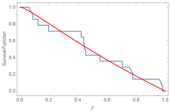
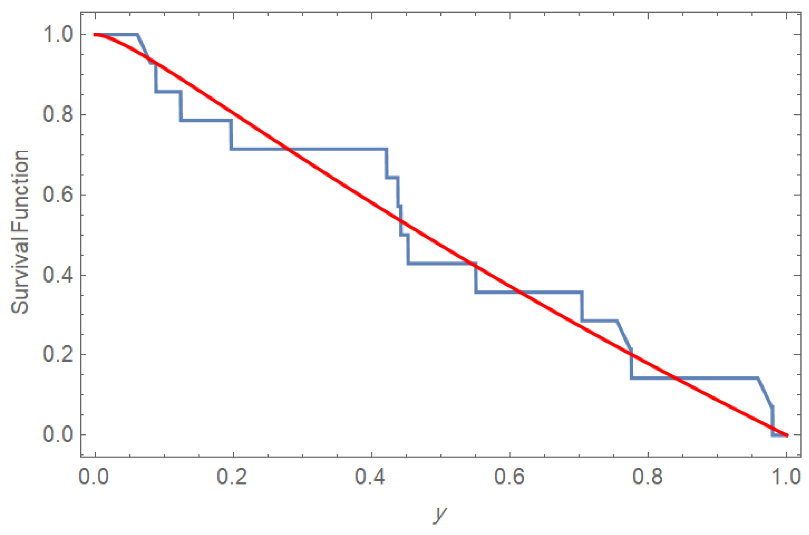
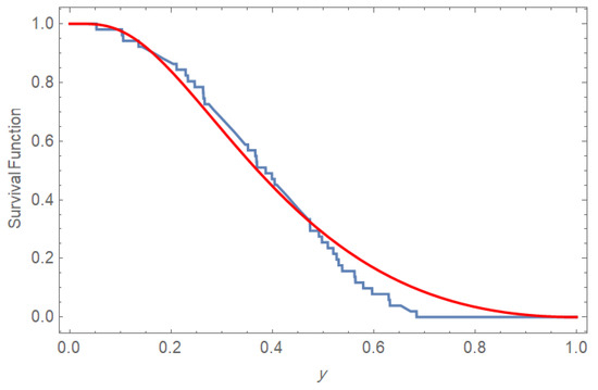
The Kolmogorov–Smirnov (K-S) test is applied to show how the ULFRD is a well-fitted model to the normalised censored values of FIMI, as displayed in Figure 4. The computed value of the K-S test is $0.157$ with a p-value equal to $0.829533$.

Figure 4. K-S test for censored FIMI data.

Table 5 shows some goodness-of-fit criteria of the ULFRD as well as the rival models, i.e., the unit Weibull, unit Lindley, and unit Kumaraswamy distributions. The findings indicate that the ULFRD provides the lowest values of AIC (Akaike Information Criterion), BIC (Bayesian Information Criterion), and HQIC (Hannan-Quinn Information Criterion) when compared to the rest of the mentioned models, which is why it can be regarded as the most suitable one to fit the FIMI dataset. The Weibull and unit Kumaraswamy models also offer quite good fits, but the unit Lindley distribution demonstrates much worse results in all aspects.

Table 5. Goodness-of-fit criteria to FIMI data.

Model	$-2\mathbf{log}\mathit{L}$	AIC	BIC	HQIC
ULFRD	$-0.28950$	$3.7105$	$4.9886$	$3.5922$
Unit Weibull	$-0.00570$	$3.9934$	$5.2715$	$3.8751$
Unit Kumaraswamy	$-0.05818$	$3.9418$	$5.2199$	$3.8235$
Unit Lindley	$69.43490$	$71.4349$	$72.074$	$71.376$

After sorting the values of FIMI and applying the developed inference approaches presented earlier in Section 4 by setting $n=19$ and $r=14$, we summarise the obtained results in Table 6.

Table 6. Inferential results from FIMI censored data.

	Point Estimates				Interval Estimates
	MLE	Bayesian SEL	Bayesian-LINEX Loss		CL	ACI	CRI
$\alpha$			$c_1=-2$	$c_2=2$	$90\%$	$0.82933,2.31287$	$1.14662,2.32358$
	$1.5711$	$1.7033$	$1.8767$	$1.5551$	$95\%$	$0.68723,2.45497$	$0.97269,2.32358$
$\beta$			$c_1=-2$	$c_2=2$	$90\%$	$-0.74635,0.30450$	$0.007336,0.13156$
	$0.22068$	$0.04379$	$0.04529$	$0.04235$	$95\%$	$-0.84706,0.40571$	$0.007336,0.13156$

According to the results presented in Table 6, the ULFR model provides comparable estimates of parameters that are consistent and interpretable, both in its classical and Bayesian estimation. The figures of the shape parameter $\alpha$ are comparatively similar in methods, which implies consistent modelling of normalised food insecurity levels despite censoring. Nevertheless, in the case of $\beta$, the Bayesian estimates are significantly smaller than the MLE, which is sensitive to the small censored sample $(n=19,r=14)$. Also, the ACIs in Table 5 contain negative lower bounds of $\beta$, which is inconsistent with the theoretical constraints of $\beta$ being positive, but the Bayesian CRIs are strictly positive and narrower. Considering that the data are socioeconomic and that reliable inferences were made to evaluate policies, the Bayesian findings reported in Table 5 seem stronger and more practical.

5.2.2. Analysis of Oil and Gas Pipeline Lifetimes

Oil and gas pipelines are usually constructed to last a few decades, typically 30–50 years. However, they will actually last according to the operating stress, environmental conditions, and corrosion in the materials. With time, pipe steel and welds develop defects, particularly with combined internal pressure, bending, and compression; hence, their lifetime is not a fixed but a probabilistic value. Kucheryavyi and Mil’kov [27] presented an experimental study about the lifetimes of certain types of pipelines, displayed as intervals of lifetimes. In this study, the midpoint of each interval is calculated and then normalised to fit the ULFRD.

The data are sorted and normalised to be in the range (0, 1), and outlier values are omitted. Therefore, n is adjusted to be 58, and r is selected to be 51.

Normalised censored values of Pipelines.
$0.0526$	$0.1028$	$0.1053$	$0.1356$	$0.1581$	$0.1685$	$0.2013$
$0.2107$	$0.2285$	$0.233$	$0.2461$	$0.263$	$0.2637$	$0.2658$
$0.2813$	$0.2987$	$0.3001$	$0.3156$	$0.3163$	$0.3332$	$0.3339$
$0.3515$	$0.366$	$0.3684$	$0.3691$	$0.3864$	$0.3989$	$0.404$
$0.4209$	$0.4216$	$0.4317$	$0.4392$	$0.4568$	$0.4646$	$0.4737$
$0.4742$	$0.4916$	$0.4974$	$0.5092$	$0.5199$	$0.5265$	$0.5305$
$0.5375$	$0.5619$	$0.5636$	$0.5791$	$0.5964$	$0.6293$	$0.6316$
$0.6621$	$0.6842$

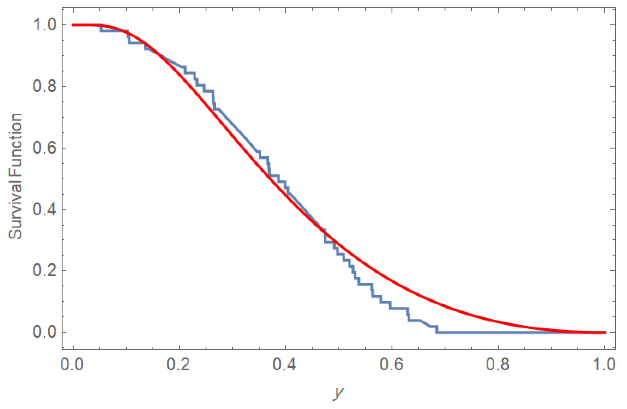
The ULFRD was tested by the K-S test against the normalised censored values of survival times, as displayed in Figure 5. The computed value of the K-S test is $0.0987057$ with a p-value equal to $0.666389$.

Figure 5. K-S test for censored pipeline data.

Despite possible minor differences in the goodness of fit to the pipeline dataset using some competing models, as displayed in Table 7, the proposed ULFRD has a structural benefit in its capacity to model bathtub-shaped hazard rate behaviour. This peculiarity is especially applicable in reliability use, where the early failure, useful life, and wear-out stages may be widely traced.

Table 7. Goodness-of-fit criteria to pipeline data.

Model	$-2\mathbf{log}\mathit{L}$	AIC	BIC	HQIC
ULFRD	$-37.8118$	$-33.8118$	$-29.9482$	$-32.3354$
Unit-Modified Weibull	$-38.3927$	$-34.3927$	$-30.529$	$-32.9163$
Unit Kumaraswamy	$-46.8061$	$-42.8061$	$-38.9424$	$-41.3297$
Unit Lindley	$-35.6976$	$-33.6976$	$-31.7658$	$-32.9594$

Based on the inferential findings, as rephrased in Table 8, we can say that the classical and Bayesian estimations of the lifetime data of the pipelines will differ noticeably. Extremities on the parameter values are more pronounced in the MLE, and the estimates under Bayesian are more moderate and consistent, which is the regularising effect of the prior in the case of censoring. It has the disadvantage of limiting the asymptotic method by including negative lower bounds of a confidence interval that are not theoretically admissible. The Bayesian CRIs, on the other hand, are always positive and narrower. In general, Table 6 indicates that Bayesian inference offers more consistent and realistic findings for censored engineering lifetime data.

Table 8. Extrapolated results from pipelines’ censored data.

	Point Estimates				Interval Estimates
	MLE	Bayesian SEL	Bayesian-LINEX Loss		CL	ACI	CRI
$\alpha$			$c_1=-2$	$c_2=2$	$90\%$	$-0.17395,0.39648$	$0.398052,1.0384$
	$0.11126$	$0.69137$	$0.73211$	$0.6522$	$95\%$	$-0.22859,0.45112$	$0.356737,1.04201$
$\beta$			$c_1=-2$	$c_2=2$	$90\%$	$0.88626,1.94981$	$0.32518,1.09737$
	$1.41803$	$0.68743$	$0.76613$	$0.6182$	$95\%$	$0.78438,2.05168$	$0.19961,1.24012$

6. Conclusions

In this paper, the ULFRD was presented to model data that is constrained within the unit interval. Some of the statistical characteristics of the distribution were obtained, such as density and hazard rate functions, moments, the characteristic function, order statistics, and Rényi entropy. Under Type-II censoring, parameter estimation was investigated under maximum likelihood and Bayesian estimation with symmetric squared error loss, and LINEX loss functions were inveztigated through a Metropolis–Hastings within the Gibbs sampling algorithm. The outcome of simulation performance showed satisfactory results of the estimators, and the generality of the model was presented on the basis of two real datasets. The practical applicability of the ULFRD was also demonstrated based on two real datasets on socioeconomic and reliability settings. The current paper has certain drawbacks: although the outcomes are promising, the empirical analysis was aimed at two datasets. Future studies can generalise the proposed model on more general censoring mechanisms as well as to proposed regression-type extensions of the proposed bounded response variables and other real-life conditions where bounded reliability or proportion-type data are encountered.

References

- Sapkota, L.P.; Bam, N.; Kumar, V. New bounded unit Weibull model: Applications with quantile regression. PLoS ONE 2025, 20, e0323888. [Google Scholar] [CrossRef] [Scilit] [PubMed]
- Abd El-Bar, A.M.T.; El-Saeed, A.R.; Karakaya, K.; Gemeay, A.M. Modeling bounded data with a new unit distribution: Regression analysis and applications. AIMS Math. 2025, 10, 17672–17704. [Google Scholar] [CrossRef] [Scilit]
- Akhtar, N.; Alharthi, M.F.; Khan, S.A.; Khan, A.A.; Amin, M. Bayesian estimation strategy for multi-component geometric life testing model under doubly type-I censoring scheme. Kuwait J. Sci. 2025, 52, 100339. [Google Scholar] [CrossRef] [Scilit]
- Akhtar, N.; Alharthi, M.F. Bayesian analysis of heterogeneous data outliers using a censored mixture model. Stat. Pap. 2025, 66, 56. [Google Scholar] [CrossRef] [Scilit]
- Mehdi, M.; Tung, Y.L.; Shahzad, M.N.; Khan, A.A.; Akhtar, N.; Alharthi, M.F. Bayesian inference for the transmuted Rayleigh distribution: Applications in behavioral data analysis. Stat. Pap. 2026, 67, 5. [Google Scholar] [CrossRef] [Scilit]
- Mazucheli, J.; Menezes, A.F.B.; Fernandes, L.B.; de Oliveira, R.P.; Ghitany, M.E. The unit-Weibull distribution as an alternative to the Kumaraswamy distribution for the modeling of quantiles conditional on covariates. J. Appl. Stat. 2019, 47, 954–974. [Google Scholar] [CrossRef] [Scilit]
- Mazucheli, J.; Menezes, A.F.; Dey, S. Unit-Gompertz distribution with applications. Statistica 2019, 79, 25–43. [Google Scholar] [CrossRef]
- Ghitany, M.E.; Mazucheli, J.; Menezes, A.F.B.; Alqallaf, F. The unit-inverse Gaussian distribution: A new alternative to two-parameter distributions on the unit interval. Commun. Stat.—Theory Methods 2019, 48, 3423–3438. [Google Scholar] [CrossRef] [Scilit]
- Gündüz, S.; Korkmaz, M.Ç. A new unit distribution based on the unbounded Johnson distribution rule: The unit Johnson SU distribution. Pak. J. Stat. Oper. Res. 2020, 16, 471–490. [Google Scholar] [CrossRef] [Scilit]
- Ribeiro-Reis, L.D. Unit log-logistic distribution and unit log-logistic regression model. J. Indian Soc. Prob. Stat. 2021, 22, 375–388. [Google Scholar] [CrossRef] [Scilit]
- ul Haq, M.A.; Hashmi, S.; Aidi, K.; Ramos, P.L.; Louzada, F. Unit modified Burr-III distribution: Estimation, characterizations and validation test. Ann. Data Sci. 2023, 10, 415–440. [Google Scholar] [CrossRef] [Scilit]
- Bakouch, H.S.; Hussain, T.; Tošić, M.; Stojanović, V.S.; Qarmalah, N. Unit Exponential Probability Distribution: Characterization and Applications in Environmental and Engineering Data Modeling. Mathematics 2023, 11, 4207. [Google Scholar] [CrossRef] [Scilit]
- Al-Omari, A.I.; Alanzi, A.R.; Alshqaq, S.S. The unit two-parameter Mirra distribution: Reliability analysis, properties, estimation and applications. Alex. Eng. J. 2024, 92, 238–253. [Google Scholar] [CrossRef] [Scilit]
- Bui, T.; Dai, S.; Singha Roy, S.; McGurk, D.; Chen, X.; Pu, S. Modified linear failure rate distribution for bathtub hazard data. J. Stat. Theory Appl. 2025, 24, 937–973. [Google Scholar] [CrossRef] [Scilit]
- Korkmaz, M.Ç.; Korkmaz, Z.S. The unit log-log distribution: A new unit distribution with alternative quantile regression modeling and educational measurements applications. J. Appl. Stat. 2021, 50, 889–908. [Google Scholar] [CrossRef] [Scilit] [PubMed]
- Sarhan, A.M.; Manshi, T.; Sobh, M.E. The unit-modified Weibull distribution: Theory, estimation, and real-world applications. Stats 2025, 8, 81. [Google Scholar] [CrossRef] [Scilit]
- Sarhan, A.M.; Sobh, M.E. Unit exponentiated Weibull model with applications. Sci. Afr. 2025, 27, e02606. [Google Scholar] [CrossRef] [Scilit]
- Barlow, R.E.; Proschan, F. Exponential life test procedures when the distribution has monotone failure rate. J. Am. Stat. Assoc. 1967, 62, 548–560. [Google Scholar] [CrossRef]
- Choudhary, N.; Tyagi, A.; Singh, B. A Flexible Bathtub-Shaped Failure Time Model: Properties and Associated Inference. Statistica 2021, 81, 65–92. [Google Scholar] [CrossRef] [Scilit]
- Gradshteyn, I.S.; Ryzhik, I.M. Table of Integrals, Series, and Products, 7th ed.; Jeffrey, A., Zwillinger, D., Eds.; Academic Press: New York, NY, USA, 2007. [Google Scholar]
- Metropolis, N.; Rosenbluth, A.W.; Rosenbluth, M.N.; Teller, A.H.; Teller, E. Equations of state calculations by fast computing machines. J. Chem. Phys. 1953, 21, 1087–1091. [Google Scholar] [CrossRef] [Scilit]
- Hastings, W.K. Monte Carlo Sampling Methods Using Markov Chains and Their Applications. Biometrika 1970, 57, 97–109. [Google Scholar] [CrossRef]
- Tierney, L.; Kadane, J.B. Accurate approximations for posterior moments and marginal densities. J. Am. Stat. Assoc. 1986, 81, 82–86. [Google Scholar] [CrossRef]
- Varian, H.R. A Bayesian approach to real estate assessment. In Studies in Bayesian Econometrics and Statistics: In Honor of L. J. Savage; Savage, L.J., Feinberg, S.E., Zellner, A., Eds.; North-Holland Pub. Co.: Amsterdam, The Netherlands, 1975; pp. 195–208. [Google Scholar]
- Mahmoud, M.A.W.; Ramadan, D.A.; Mansour, M.M.M. Estimation of lifetime parameters of the modified extended exponential distribution with application to a mechanical model. Commun. Stat.—Simul. Comput. 2022, 51, 7005–7018. [Google Scholar] [CrossRef] [Scilit]
- Elzaki, R.M.; Al-Mahish, M. Food insecurity and water management shocks in Saudi Arabia: Bayesian VAR analysis. PLoS ONE 2024, 19, e0296721. [Google Scholar] [CrossRef]
- Kucheryavyi, V.I.; Mil’kov, S.N. Statistical modeling of the oil and gas pipeline lifetime under bending and compression. J. Mach. Manuf. Reliab. 2013, 42, 341–346. [Google Scholar] [CrossRef] [Scilit]
Disclaimer/Publisher’s Note: The statements, opinions and data contained in all publications are solely those of the individual author(s) and contributor(s) and not of MDPI and/or the editor(s). MDPI and/or the editor(s) disclaim responsibility for any injury to people or property resulting from any ideas, methods, instructions or products referred to in the content. |
© 2026 by the authors. Licensee MDPI, Basel, Switzerland. This article is an open access article distributed under the terms and conditions of the Creative Commons Attribution (CC BY) license.