DecompPatchTST: A Hybrid Framework Fusing Learnable Polynomials and Patch Transformers for Time-Series Forecasting

Abstract

In real-world data, the structural symmetry of time series across temporal scales is often disrupted by the entanglement of trend, seasonal, and high-frequency components. This poses significant challenges to reliable time-series forecasting (TSF) in applications like power dispatch and meteorological analysis. Transformer-based methods typically model mixed signals without explicit inductive bias, while current decomposition-based approaches often rely on linear approximations for trend evolution, leading to unstable extrapolation in long-term forecasting. To overcome these challenges, this paper proposes the Decomposition Patch Time Series Transformer (DecompPatchTST), a hybrid forecasting framework integrating decomposition, trend extrapolation, and patch-based representation. A moving-average operator first decomposes the sequence into trend and residual parts. The trend is extrapolated via a learnable polynomial basis, which adaptively models complex nonlinear trends to ensure smooth long-range dynamics, whereas the residual is divided into temporal patches and modeled by a shared transformer encoder to capture seasonal and high-frequency variations. The final forecast aggregates both components through an additive structure. Experiments on ETT datasets show that DecompPatchTST is more stable with relatively smoother error growth from 96 to 720 forecasting steps. Its practical performance is further demonstrated on real-world Australian electricity data.

1. Introduction

Time-series forecasting (TSF) is crucial in fields such as power load planning [1], financial analysis [2] and meteorological monitoring [3]. Its core objective is to extract patterns from historical sequences to predict future states [4]. Time series often exhibit implicit symmetries across different temporal scales, including translational symmetry over seasonal periods, scale symmetry in trend evolution, and structural symmetry between the decomposition of a series into interpretable components and its subsequent reconstruction. With the development of smart grids and energy internet, accurate and stable long-term forecasting of power loads and prices has become essential for ensuring the safe operation of power systems. However, real-world sequences typically contain overlapping trends, seasonal structures, and high-frequency noise, entangling components across scales and disrupting the inherent structural symmetry of the series. This poses significant challenges to the accuracy and stability of long-term forecasting [1]. Therefore, constructing models that effectively disentangle these components to restore structural symmetry while maintaining stability over extended prediction windows not only possesses theoretical research value but also bears practical significance for applications like energy management.

TSF methods have evolved from traditional statistical modeling to deep learning methods. Early research primarily relied on statistical and machine learning methods like Autoregressive Integrated Moving Average (ARIMA) [5]. These methods are based on linear relationships and perform reasonably well on structurally simple or short-term forecasting tasks, but they struggle to model nonlinear variations and multiscale dynamics prevalent in real-world scenarios [6]. To enhance nonlinear modeling capability, researchers introduced deep learning-based predictive models. Among these, Recurrent Neural Network (RNN) [7] variants like Long Short-Term Memory (LSTM) [8] and Gated Recurrent Unit (GRU) [9] have been widely applied to multivariate TSF through gating mechanisms. Concurrently, Convolutional Neural Networks (CNNs) [10] leverage local receptive fields to extract short-term dynamic features, achieving notable results in capturing local fluctuations. With increasing demand for long-term forecasting, the transformer [11] architecture was introduced to time-series prediction due to its self-attention mechanism [11], which enables direct modeling of global temporal dependencies. This led to a series of improved models, such as iTransformer [12] and FEDformer [13], which enhance long-sequence modeling efficiency through strategies such as frequency-domain analysis. Subsequent research has further diversified the architectural landscape, with models like TimesNet [14] leveraging multi-periodicity, Crossformer [15] capturing cross-dimension dependencies, and TSMixer [16] exploring efficient MLP-based designs for temporal modeling. In addition, emerging architectures, such as state-space sequence models represented by Mamba [17] and large-scale forecasting models such as Chronos [18] and Time-LLM [19], further expand the modeling paradigms for time-series analysis.

Despite the rapid progress of deep learning models for time-series forecasting, many methods still treat raw time series as unified inputs for holistic modeling. The issue of interference between components at different time scales persists. To enhance the inductive bias toward temporal structure, some studies have begun incorporating time-series decomposition concepts [20] by explicitly decomposing the raw sequence into trend, seasonal, and residual components for separate modeling. For instance, DLinear [21] employs moving-average decomposition [4] followed by linear mapping of each component, significantly improving computational efficiency. However, several limitations remain. On the one hand, trend components in many decomposition-based methods rely on simple linear mapping, struggling to fit complex nonlinear trends. On the other hand, residual components typically mix different variables without further decoupling, hindering the model’s ability to capture short-term dynamics and cyclical structures.

To address these challenges, this paper proposes the DecompPatchTST model, a hybrid forecasting architecture that integrates time-series decomposition with the PatchTST modeling mechanism. The core philosophy is to restore the structural symmetry of time series by explicitly separating the entangled components and modeling each with an inductive-biased module, followed by a symmetric reconstruction. The model comprises a time-series decomposition module, polynomial trend extrapolation module, and PatchTST [22] encoding module. The main contributions of this paper can be summarized as follows:

(1)

DecompPatchTST is proposed to model long-term trends, periodic patterns, and short-term fluctuations more effectively. The original series is decomposed into trend and residual components, thereby mitigating cross-scale interference among heterogeneous temporal dynamics.

(2)

Comparative evaluations are conducted on four ETT benchmark datasets against seven representative time-series forecasting models, and ablation studies are performed to verify the contribution of each module.

(3)

The practical utility of the proposed model is further validated on real-world Australian electricity load and price datasets. The results demonstrate that the model achieves stable forecasts while maintaining strong performance under realistic conditions.

The structure of this paper is as follows: Section 2 introduces related works on time-series prediction, Section 3 presents the preliminaries, Section 4 describes the DecompPatchTST model, Section 5 describes the experiments, and Section 6 concludes the paper.

2. Related Work

2.1. Traditional Statistical and Machine Learning Methods

Early TSF primarily relied on traditional statistical and machine learning methods. Classical models such as the Seasonal Autoregressive Integrated Moving Average (SARIMA) [23] aim to make series stationary and capture trend and periodic features through differencing and linear autocorrelation structures. As research progressed, Vector Autoregression (VAR) [24] and state-space models (SSMs) [17] were proposed to capture dynamic correlations among multivariate series. However, these models typically rely on linear assumptions, which limits their ability to adapt to the complex, non-stationary, and nonlinear temporal structures observed in the real world. To overcome these linear limitations, machine learning methods such as Support Vector Regression (SVR) [25] and Extreme Gradient Boosting (XGBoost) [26] were introduced, incorporating nonlinear representational capacity via kernel functions or tree ensembles. Although these methods perform well for short-term forecasting, they often depend on recursive multi-step forecasting for long-term tasks, which can lead to error accumulation as the prediction horizon increases [27,28], thereby limiting long-term forecasting performance. In contrast, our model employs a learnable polynomial module to directly model nonlinear trends and adopts a non-recursive decomposition-based forecasting paradigm to mitigate error propagation.

2.2. TSF Models Based on Recurrent and Convolutional Networks

To overcome the limitations of traditional methods in nonlinear modeling and error accumulation, researchers introduced RNNs [7], which update hidden states recursively to capture temporal dependencies. Their variants, LSTM [8] and GRU [9,29], effectively mitigate gradient vanishing and explosion problems through gating mechanisms. However, the temporal order dependency of RNN forward computation hinders parallelization, limiting their capability for long-sequence modeling. In contrast, CNNs leverage the parallelism of convolutional operations and local receptive fields to effectively extract local features. SCINet [30] utilizes hierarchical convolution to achieve multi-scale feature extraction, effectively capturing information at different time scales within a series. TimesNet [14] transforms one-dimensional sequences into two-dimensional structures for modeling. Although CNNs excel at capturing local patterns, their convolutional layers have limited receptive fields. Modeling long sequences requires techniques like dilated convolution to expand the receptive field [31,32], making it difficult to effectively model global long-range dependencies. In contrast to the sequential processing of RNNs and the local receptive fields of CNNs, the proposed method leverages patch-based attention mechanisms to achieve global dependency modeling, which is suitable for long-term forecasting tasks.

2.3. TSF Models Based on Transformer

The introduction of transformer [11] provided a new method for capturing long-range dependencies. Its self-attention mechanism can capture dependencies between any positions globally, significantly enhancing long-sequence modeling capability and effectively solving the problem of limited receptive fields in CNNs. On this basis, many improved models have been proposed by researchers [33]. FEDformer [13] employs frequency-domain sparse attention to retain low-frequency components, thereby reducing computational cost and improving forecasting efficiency. Crossformer [15] adopts a dual-layer attention structure across time and across variables for multivariate dependency modeling. PatchTST effectively alleviates the computational burden of attention through patching and channel-independent design [22]. iTransformer [12] treats time steps as tokens and variables as features, enabling effective modeling in the cross-variable direction. These models have made significant breakthroughs in capturing long-range dependencies, but they often lack inductive bias towards the inherent structure of the series. They cannot explicitly distinguish between trend, periodic, and random noise components, which may lead to interference between heterogeneous temporal patterns. The proposed method introduces explicit decomposition to alleviate this issue and enhance modeling stability.

2.4. TSF Models Based on Decomposition

To address the lack of structural inductive bias and high computational cost in transformer-based models, some studies have introduced decomposition strategies into model design [34]. Autoformer [35] decomposes the series into trend and seasonal components and models them via an autocorrelation mechanism, which effectively enhances temporal modeling capability. Building on this, to further improve computational efficiency and simplicity, researchers proposed the DLinear model [21]. It employs moving averages to decompose the original series into trend and seasonal branches and uses linear layers for separate prediction. This decomposition-based linear modeling strategy introduces inductive bias while significantly reducing computational cost, demonstrating excellent forecasting performance in long-term TSF tasks.

The above review reveals that, despite their advantages in modeling long-term dependencies and incorporating structural inductive bias, the current methods still face challenges in real-world scenarios. First, the existing decomposition methods for trend component modeling remain relatively simple, making it difficult to capture complex long-term evolution patterns. Second, different short-term structures within residual components, such as seasonal fluctuations and high-frequency noise, are often modeled jointly, which reduces modeling precision. To address these challenges, this paper proposes the DecompPatchTST model. For nonlinear trend modeling, the proposed model replaces fixed linear mappings with a polynomial trend extrapolation module that fits temporal basis functions using learnable coefficients [36,37], enabling stable extrapolation of complex long-term trends. [38] For residual modeling, the model combines a PatchTST encoder with a dual prediction head architecture to explicitly decouple seasonal structures and high-frequency noise, thereby improving short-term dynamic modeling while maintaining computational efficiency.

3. Preliminaries

3.1. Problem Definition

TSF aims to predict future values based on historical observations. Given a historical observation sequence of length $L$, denoted as $\mathit{X}=\left[x_1, x_2, \dots , x_L\right]\in {ℝ}^{L\times V}$, where $V$ represents the number of variables, the objective is to learn a mapping function $f\left(·\right)$ that infers future values $\mathit{Y}=\left[x_{L+1}, x_{L+2}, \dots , x_{L+T}\right]\in {ℝ}^{T\times V}$ over a prediction horizon of length $T$. The forecasting problem is formally defined as

$$\mathit{Y}=f\left(X;\theta \right)$$

(1)

where $\theta$ denotes the learnable parameters of the model. In this case, the model must not only learn complex nonlinear dynamics but also robustly capture trend evolution, seasonal patterns, and short-term disturbances.

3.2. Time-Series Decomposition

In complex forecasting tasks, multivariate time series are often non-stationary and consist of components operating at different temporal scales. These components interact with each other, making direct modeling difficult and prone to overfitting. To address this issue, this paper adopts time-series decomposition to divide complex non-stationary series into relatively stable and interpretable components. The classical additive decomposition model [20] represents a time series as

$${\mathit{X}}_t={\mathit{T}}_t+{\mathit{S}}_t+{\mathit{R}}_t$$

(2)

where ${\mathit{X}}_t$ denotes the observed value, ${\mathit{T}}_t$ represents the slowly varying trend component, ${\mathit{S}}_t$ denotes the seasonal component with periodic patterns, and ${\mathit{R}}_t$ represents high-frequency random noise. Additive decomposition is widely used in statistical modeling, signal processing, and forecasting systems as it provides a structured representation that aligns with human understanding and allows models to focus more effectively on predictable components.

3.3. Additive Invariance

Additive invariance characterizes the structural symmetry between decomposition and reconstruction as the relationship maintained between decomposing a time series into independent components and aggregating the predictions of these components to reconstruct the overall forecast. The decomposition operator $D$ maps the observed quantity $\mathit{X}$ to a set of components ${\left\{{\mathit{C}}_{\mathrm{k}}\right\}}_{\mathrm{k}=1}^K$. The invariance property is defined by the reconstruction constraint

$$\mathit{X}={\displaystyle {\displaystyle \sum _{\mathrm{k}=1}^K}{\mathit{C}}_{\mathrm{k}}}$$

(3)

where $\mathrm{k}$ denotes the number of components obtained from the decomposition and ${\mathit{C}}_{\mathrm{k}}$ denotes the k-th component. Complex dynamics can be modeled by learning independent mapping functions $f_{\mathrm{k}}\left(\cdot \right)$ for each component. Thus, the final forecast $\stackrel{\wedge }{\mathit{Y}}$ preserves this additive structure as follows:

$$\stackrel{\wedge }{\mathit{Y}}={\displaystyle {\displaystyle \sum _{\mathrm{k}=1}^K}{f}_{\mathrm{k}}\left({\mathit{C}}_{\mathrm{k}}\right)}$$

(4)

thereby maintaining structural symmetry between the decomposition and reconstruction processes. The series can therefore be represented as a sum of separable component functions, allowing independent modeling while predicting.

3.4. Transformer Encoder

The transformer architecture captures dependencies between arbitrary time steps through self-attention mechanisms. Unlike RNNs, transformers can process entire sequences in parallel, making them more efficient for long-sequence forecasting. Transformer encoder layer consists of a multi-head self-attention (MHSA) module and a Feed-Forward Network (FFN), combined with residual connections and layer normalization to facilitate deep network training [11].

Given an input sequence $\mathit{Z}=\left[z_1, z_2, \dots , z_N\right]\in {ℝ}^{L\times d}$ to the transformer encoder, where $d$ is the model dimension, linear projections are first applied to generate query, key, and value matrices as follows:

$$\mathit{Q}={\mathit{Z}\mathit{W}}_Q, \mathit{K}={\mathit{Z}\mathit{W}}_K, \mathit{V}={\mathit{Z}\mathit{W}}_V$$

(5)

where ${\mathit{W}}_Q,{\mathit{W}}_K\in {ℝ}^{d\times d_k}$, ${\mathit{W}}_V\in {ℝ}^{d\times d_v}$ are learnable parameters. For each attention head $h$, attention weights and outputs are computed as

$$\mathit{h}\mathit{e}\mathit{a}{\mathit{d}}_h=\mathrm{Attention}\left({\mathit{Q}}_h,{\mathit{K}}_h,{\mathit{V}}_h\right)=\mathrm{softmax}\left({\displaystyle \frac{{\mathit{Q}}_h{\mathit{K}}_h^T}{\sqrt{d_k}}}\right){\mathit{V}}_h$$

(6)

where $\sqrt{d_k}$ is a scaling factor used to stabilize training. Outputs from all attention heads are concatenated and projected to form the final multi-head attention output:

$$\mathrm{MultiHead}\left(\mathit{Q},\mathit{K},\mathit{V}\right)=\left[{\mathit{h}\mathit{e}\mathit{a}\mathit{d}}_1, {\mathit{h}\mathit{e}\mathit{a}\mathit{d}}_2, \dots , {\mathit{h}\mathit{e}\mathit{a}\mathit{d}}_h\right]{\mathit{W}}^O={\mathit{Z}}^{\prime }$$

(7)

where ${\mathit{W}}^O\in {ℝ}^{h·d_v\times d}$ denotes the output projection matrix and $h$ is the number of attention heads. Subsequently, the output of the MHSA layer is passed through a residual connection and layer normalization to alleviate gradient vanishing, forming the output of the first sublayer:

$${\mathit{Z}}_{norm}=\mathrm{LayerNorm}\left(\mathit{Z}+{\mathit{Z}}^{\prime }\right)$$

(8)

and then the ${\mathit{Z}}_{norm}$ is fed into the FFN. The FFN consists of two linear transformations and a nonlinear activation function ReLU, and its purpose is to perform nonlinear transformation and dimension adjustment on the features extracted by the self-attention mechanism. The FFN operation is defined as follows:

$$\mathrm{FFN}\left({\mathit{Z}}_{norm}\right)=\mathrm{ReLU}\left({\mathit{Z}}_{norm}{\mathit{W}}_1+b_1\right){\mathit{W}}_2+b_2$$

(9)

where ${\mathit{W}}_1\in {ℝ}^{d\times d_{ff}}, b_1\in {ℝ}^{d_{ff}}, {\mathit{W}}_2\in {ℝ}^{d_{ff}\times d}, b_2\in {ℝ}^d$ are learnable parameters, and $d_{ff}$ denotes the hidden dimension inside the FFN. The output of the FFN is also passed through a residual connection and layer normalization to produce the final output of the transformer encoder:

$${\mathit{Z}}_{output}=\mathrm{LayerNorm}\left({\mathit{Z}}_{norm}+\mathrm{FFN}\left({\mathit{Z}}_{norm}\right)\right)$$

(10)

3.5. PatchTST

PatchTST is a transformer variant designed for long-sequence forecasting. Different from traditional attention mechanisms, the core of PatchTST lies in patch segmentation and channel independence [22]. Through the patching operation, the time series is divided into local segments to address the quadratic computational complexity of traditional transformers when processing long sequences [39], while the channel independence strategy is adopted to effectively capture multivariate variables. Specifically, PatchTST splits the time series into multiple smaller patches and processes them independently. Given a multivariate time-series input $\mathit{X}=\left[x_1, x_2, \dots , x_T\right]\in {ℝ}^{T\times D}$, where $T$ denotes the length of time steps and $D$ denotes the number of variables, the input sequence is divided into subsequence patches with length L and stride S as follows: ${\mathit{P}}_i={\mathit{X}}_{iS : iS + L}\in {ℝ}^{L\times D}, i=0, 1, \dots , N-1$, where $N=⌊{\displaystyle \frac{T-L}{S}}⌋+1$ represents the number of patches. This operation reduces the effective sequence length, and the computational complexity is reduced from $O\left(T^2\right)$ to $O\left(N^2\right)$ [11,39], thereby improving computational efficiency. The patch sequence corresponding to each variable is projected into the model space through a linear projection and combined with positional encoding to preserve temporal information:

$${\mathit{Z}}_0^{\left(i\right)}={\mathit{W}}_p{\mathit{P}}^{\left(i\right)}+{\mathit{W}}_{pos}$$

(11)

where ${\mathit{W}}_p$ denotes the projection weight and ${\mathit{W}}_{pos}$ represents the positional encoding [22]. Subsequently, the resulting embedding matrix $\mathit{Z}$ serves as the input for transformer encoder, bridging the raw input features with the attention mechanism. The encoded representations of all variables are processed by a shared transformer encoder for feature extraction. Finally, each variable generates predictions for the future $T$ time steps through an independent prediction head, and these predictions together form the final multivariate forecasting result ${\mathit{Y}}_{pred}$.

4. Methods

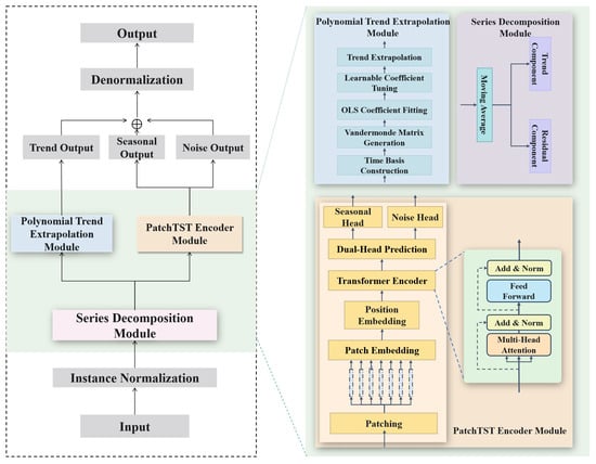
This section describes the overall architecture of DecompPatchTST. As shown in Figure 1, the model consists of three core modules, forming a process designed to restore structural symmetry through disentanglement and specialized modeling. First, the series decomposition module explicitly decomposes the input time series into trend and residual components using a moving-average operator. Second, the polynomial trend extrapolation module extrapolates the decomposed trend component by modulating polynomial basis functions with learnable coefficients. Third, the PatchTST encoder module processes the residual sequence through patch segmentation and a shared transformer encoder, followed by dual prediction heads to further disentangle and capture the translational symmetry of seasonal patterns and the irregular nature of noise. Finally, the predicted trend, seasonal, and noise components are aggregated through an additive structure that mirrors the initial decomposition to obtain the final forecasting result, thereby completing the symmetry restoration. During training, the model parameters are optimized using the AdamW optimizer with Mean Squared Error as the loss function.

Figure 1. Overall architecture of DecompPatchTST.

4.1. Series Decomposition Module

Original time series often entangle trend, seasonal, and noise components, breaking the inherent structural symmetry and increasing the difficulty of direct modeling. To address this issue, a moving-average (MA) operator is employed to decompose the input sequence into trend and residual components. Unlike Seasonal-Trend decomposition using LOESS (STL), which requires explicit seasonal period specification and iterative smoothing procedures, moving-average filtering provides a lightweight and stable trend extraction mechanism. Compared with learnable decomposition strategies, it does not introduce additional trainable parameters, thereby preserving model simplicity and reducing the risk of overfitting. The trend component $\mathit{T}$ is computed using a centered moving average with window size $k$, which is set as 25:

$${\mathit{T}}_t={MA}_k\left({\mathit{x}}_t\right)={\displaystyle \frac{1}{k}}{\displaystyle {\displaystyle \sum _{i=-m}^m}{\mathit{x}}_{t+i}}$$

(12)

where ${\mathit{T}}_t$ denotes the estimated trend value at time step $t$, ${MA}_k\left(·\right)$ denotes the moving-average operator, and $m={\displaystyle \frac{k-1}{2}}$ indicates the window radius. Specifically, for each time step, the average of the preceding and succeeding $m$ samples is computed as the trend value. This operator functions as a low-pass filter, suppressing high-frequency noise and extracting low-frequency components. The smoothed trend term effectively captures long-term variations, and subtracting the trend from the original series yields the residual term ${\mathit{x}}_t-{\mathit{T}}_t$. The resulting trend component $\mathit{T}$ and residual component $\mathit{R}$ are subsequently fed into the polynomial trend extrapolation module and the PatchTST encoder module, respectively.

4.2. Polynomial Trend Extrapolation Module

This module takes the $\mathit{T}\in {ℝ}^{B\times S\times V}$ from the series decomposition module as input, where $B$ is the batch size, $S$ is the lookback window length, and generates the trend forecast $\stackrel{\wedge }{\mathit{T}}\in {ℝ}^{B\times L\times V}$ for the next $L$ time steps. Considering the smooth and low-frequency characteristics of the trend component, we adopt a polynomial extrapolation method. According to the Weierstrass approximation theorem, for any continuous function $f\left(\mathrm{t}\right)$ defined on a closed interval $\left[a,b\right]$ and any $\epsilon <0$, there exists a polynomial $P_n\left(t\right)$ of degree $n$ such that

$$\underset{t\in \left[a,b\right]}{\sup }\left|f\left(t\right)-P_n\left(t\right)\right|<\epsilon$$

(13)

thus, polynomial bases can uniformly approximate continuous trend functions on bounded intervals. The core of this module comprises three key steps: construction of time basis functions, least squares fitting with learnable coefficient modulation, and extrapolative forecasting.

First, the historical time point $t=1, 2, \dots , S$ and future time points $t=S+1, \dots , S+L$ are normalized to the interval $\left[-1, 1\right]$, yielding normalized coordinates ${\mathit{t}}_{in}={\left[t_1, t_2, \dots , t_S\right]}^{\mathrm{T}}$ and $t_{out}={\left[t_{S+1}, t_{S+2}, \dots , t_{S+L}\right]}^{\mathrm{T}}$. This normalization maps the input to a bounded range, preventing ill-conditioned basis matrices caused by large raw time values, which is critical for stability. The corresponding polynomial basis matrices are constructed as

$$\begin{array}{c}{\mathit{X}}_{in}=\left[\begin{array}{ccccc}1& t_1& t_1^2& \cdots & t_1^d\\ 1& t_1& t_2^2& \cdots & t_2^d\\ ⋮& ⋮& ⋮& \ddots & ⋮\\ 1& t_S& t_S^2& \cdots & t_S^d\end{array}\right]\in {ℝ}^{S\times \left(d+1\right)}\\ \\ {\mathit{X}}_{out}=\left[\begin{array}{ccccc}1& t_{S+1}& t_{S+1}^2& \cdots & t_{S+1}^d\\ 1& t_{S+2}& t_{S+2}^2& \cdots & t_{S+2}^d\\ ⋮& ⋮& ⋮& \ddots & ⋮\\ 1& t_{S+L}& t_{S+L}^2& \cdots & t_{S+L}^d\end{array}\right]\in {ℝ}^{L\times \left(d+1\right)}\end{array}$$

(14)

where $d$ is the polynomial degree. Although increasing the polynomial degree can improve historical fitting accuracy, it risks overfitting by capturing high-frequency noise instead of the underlying trend evolution. This leads to severe oscillations in the prediction interval and a decline in generalization capability. We set $d=3$, a value determined through validation-set evaluation over $d\in \left\{2, 3, 4\right\}$. This low degree avoids numerical instability and excessive oscillations, ensuring smooth and bounded trend evolution. Next, the ordinary least squares (OLS) method is used to fit the polynomial coefficients $\beta$ to the historical trend. In cases where the matrix is irreversible, the Moore–Penrose pseudo-inverse is employed for computation:

$$\mathit{\beta }={\mathit{X}}_{in}^{+}\mathit{T}$$

(15)

where ${\mathit{X}}_{in}^{+}$ is the pseudo-inverse of the historical time basis matrix. This approach ensures a stable solution even when the basis matrix is ill-conditioned or near-singular. Subsequently, a learnable linear transformation layer is introduced to modulate the coefficients:

$${\mathit{\beta }}^{\prime }=\mathit{W}\mathit{\beta }+\mathit{b}$$

(16)

where $\mathit{W}$ and $\mathit{b}$ are learnable parameters. Unlike methods using independent loss functions for coefficient fitting, this layer is trained jointly with the entire model via the final prediction loss, ensuring that the trend extrapolation is directly optimized for the ultimate forecasting objective. Finally, the predicted future trend $\stackrel{\wedge }{\mathit{T}}$ for the next $L$ steps is generated using the future time basis matrix ${\mathit{X}}_{out}$ and the learned coefficients:

$$\stackrel{\wedge }{\mathit{T}}={\mathit{X}}_{out}{\mathit{\beta }}^{\prime }\in {ℝ}^{B\times L\times V}$$

(17)

4.3. PatchTST Encoder Module

The PatchTST encoder module processes the residual component $\mathit{R}$ obtained from the series decomposition module. Although the residual component $\mathit{R}$ is a single signal, the model employs a shared encoder and a dual-head prediction architecture to implicitly decouple it into a predictable seasonal component and a noise component without requiring any explicit secondary decomposition. First, the residual sequence $\mathit{R}$ is segmented into fixed-length temporal patches. Each patch is mapped into a unified vector space via linear projection and positional encoding. The encoded patch sequence is then fed into a shared transformer encoder for further processing. After processing through multiple layers, the last hidden state vector of the output sequence is taken as the aggregated representation of the entire historical residual series. This representation is fed into two independent linear prediction heads, designated for predicting the seasonal component $\stackrel{\wedge }{\mathit{S}}$ and the noise component $\stackrel{\wedge }{\mathit{N}}$:

$$\stackrel{\wedge }{\mathit{S}}={\mathit{W}}_S•\mathit{h}+{\mathit{b}}_S$$

(18)

$$\stackrel{\wedge }{\mathit{N}}={\mathit{W}}_N•\mathit{h}+{\mathit{b}}_N$$

(19)

where ${\mathit{W}}_S$ and ${\mathit{W}}_N$ are the linear transformation matrices for the seasonal and noise components, respectively, and ${\mathit{b}}_S$ are the corresponding bias terms. The noise component refers to predictable high-frequency or irregular variations learned jointly with the seasonal component from the shared residual representation, optimized solely via the final MAE loss and without any separate ground-truth labels. The patching mechanism, channel-independent design, and dual prediction heads collectively reduce computational complexity and accurately capture periodic and irregular variations, thereby improving overall forecasting performance. The detailed execution flow of this module is outlined in Algorithm 1. The final outputs $\stackrel{\wedge }{\mathit{S}}$ and $\stackrel{\wedge }{\mathit{N}}$ are used for the final aggregation.

Algorithm 1. The PatchTST Encoder Module Process

Input: R(B, S, V) Output: S: (B, L, D)       N: (B, L, D)

1: P: (B, N, L×V)           ← patchify(R) 2: E: (B, N, Dmodel)    ← Linear(P)    {Patch embedding projection} 3: Z: (B, N, Dmodel)    ← E + PositionalEncoding   {Add position information} 4: Q, K, V: (B, N, Dk)   ← Linear(Z),Linear(Z),Linear(Z)   {Project to query, key, value} 5: A: (B, N, N)       ← $\mathrm{softmax}\left({\displaystyle \frac{\mathit{Q}{\mathit{K}}^T}{\sqrt{D_k}}}\right)$    {compute self-attention weights} 6: Z′: (B, N, Dmodel) ← Linear(A × V)  {Multi-head attention output} 7: Z″: (B, N, Dmodel) ← LayerNorm(Z + Z′)    {Add&Norm} 8: Zffn: (B, N, Dmodel) ← FFN(Z″)    {Feed-forward network} 9: Zout: (B, N, Dmodel) ← LayerNorm(Z″ + Zffn)  {Add&Norm} 10: $\stackrel{\wedge }{\mathit{S}}$: (B, L, D) ← Linear(Zout)            {Seasonal output prediction} 11: $\stackrel{\wedge }{\mathit{N}}$: (B, L, D) ← Linear(Zout)           {Noise output prediction}

4.4. Output Aggregation and Denormalization

This module functions as the final output layer of the model by integrating the predictions from the three components: trend, seasonality, and noise. It also maps the normalized predictions back to the original data scale to generate the final forecast sequence that possesses physical meaning. Specifically, the model aggregates the three predictive components using the following equation to obtain the final forecast, mirroring the initial additive decomposition assumption and thereby restoring structural symmetry:

$$\stackrel{\wedge }{\mathit{Y}}=\stackrel{\wedge }{\mathit{T}}+\stackrel{\wedge }{\mathit{S}}+\stackrel{\wedge }{\mathit{N}}$$

(20)

where $\stackrel{\wedge }{\mathit{T}}, \stackrel{\wedge }{\mathit{S}}, \stackrel{\wedge }{\mathit{N}}$ represent the predicted values of the trend, seasonal, and noise components from the previous modules, respectively. This additive synthesis method ensures that the model effectively utilizes the independent characteristics of each component during forecasting and maintains consistency with the initial assumed decomposition structure. To restore the model’s predictions to the original data space, we perform a denormalization process. During training, all input data underwent standardization processing, meaning each instance ${\mathit{X}}_i$ was normalized as follows:

$${\stackrel{\wedge }{\mathit{X}}}_i^{norm}={\displaystyle \frac{{\mathit{X}}_i-{\mu }_{{\mathit{X}}_i}}{{\sigma }_{{\mathit{X}}_i}}}$$

(21)

where ${\mu }_{{\mathit{X}}_i}$ and ${\sigma }_{{\mathit{X}}_i}$ represent the mean and standard deviation of the input data, respectively. To recover the original data scale, denormalization is performed as follows:

$${\stackrel{\wedge }{\mathit{X}}}_i^{final}={\stackrel{\wedge }{\mathit{X}}}_i^{norm}\times {\sigma }_{{\mathit{X}}_i}+{\mu }_{{\mathit{X}}_i}$$

(22)

where ${\stackrel{\wedge }{\mathit{X}}}_i^{final}$ is the final denormalized prediction value, representing the model’s ultimate output for instance. Through this denormalization process, the model’s output is converted back to the same measurement units as the input data, facilitating meaningful comparison and evaluation against actual observed values.

5. Experiments

To validate the effectiveness of the proposed model in multivariate TSF, experiments were conducted on four public datasets, and comparisons were made with existing baseline models.

5.1. Datasets and Baseline Models

To evaluate the proposed model, experiments were performed on the ETT (Electricity Transformer Temperature) benchmark dataset [35]. This dataset is sourced from two electricity transformers in China, recorded from July 2016 to July 2018, and includes seven operating indicators, such as load and oil temperature, reflecting the operational status of electrical equipment in real industrial environments. It contains four subsets: two with 1-hour intervals (ETTh1 and ETTh2), which exhibit long-term trends with weekly and monthly periodicity; and two with 15-minute intervals (ETTm1 and ETTm2), which capture higher-frequency fluctuations. From a statistical perspective, the data exhibit clear non-stationary characteristics with slowly varying long-term trends and pronounced weekly periodicity. Moreover, the ETTm dataset demonstrates stronger high-frequency volatility due to operational disturbances and measurement noise. This dataset is therefore ideal for validating the model’s robustness against trends, periodicity, and noise interference. The dataset contains no missing values. We performed data preprocessing, including normalization and chronological segmentation. The training, validation, and test sets are proportioned approximately 6:2:2. Specific details of each dataset are presented in Table 1.

Table 1. Overview of the experimental datasets.

Dataset	Channels	Prediction Length	Dataset Split	Granularity	Domain
ETTh1	7	{96, 192, 336, 720}	(8545, 2881, 2881)	60 min	Electricity
ETTh2	7	{96, 192, 336, 720}	(8545, 2881, 2881)	60 min	Electricity
ETTm1	7	{96, 192, 336, 720}	(34,465, 11,521, 11,521)	15 min	Electricity
ETTm2	7	{96, 192, 336, 720}	(34,465, 11,521, 11,521)	15 min	Electricity

The proposed model was compared with six representative forecasting models, as summarized in Table 2: (1) models based on recurrent and convolutional networks: SCINet [30]; (2) long-term TSF models based on transformers: FEDformer [13], PatchTST [22], and Autoformer; (3) time-series forecasting models based on linear [40] and MLP [41,42] approaches: DLinear [21], TSMixer [16], and TiDE [43]. Brief descriptions of these models are as follows:

Table 2. Comparison between our model and other related baselines.

Models	Architecture Type				Decomposition	Complexity
	CNN	MLP	Linear	Transformer		Low	Medium	High
TiDE		✔				✔
FEDformer				✔	✔		✔
SCINet	✔						✔
Dlinear			✔		✔	✔
TSMixer		✔				✔
PatchTST				✔			✔
Autoformer				✔	✔			✔

TiDE: An encoder–decoder model based on multilayer perceptron (MLP).

FEDformer: Maps sequences to the frequency domain through Fourier transform and implicitly models trends and periodic patterns in sequences using frequency components, significantly reducing computational complexity while effectively improving long-sequence forecasting efficiency. SCINet: A time-series forecasting model based on multi-resolution downsampling and convolutional interaction, capturing complex temporal patterns by recursively decomposing sequences into odd–even subsequences and applying interactive learning.

DLinear: A linear model for the time-series forecasting field, with a core design that decomposes input sequences into trend and residual components and uses two independent linear layers for separate modeling and prediction.

TSMixer: Alternately mixes information across time and feature dimensions to quickly capture complex dependencies in multivariate series.

PatchTST: Segments time series into subsequence patches and models them with channel independence.

Autoformer: Internally decomposes series and employs autocorrelation to capture periodic patterns, enhancing long-term forecasting stability.

5.2. Evaluation Metrics and Loss Function

This paper employs Mean Absolute Error (MAE) and Mean Squared Error (MSE) [12] as evaluation metrics for the model.

5.2.1. Mean Absolute Error (MAE)

MAE calculates the average of the absolute differences between the predicted values and the actual values. Given a batch of data containing $\mathit{N}$ samples, for a single sample within it, the predicted output is ${\stackrel{\wedge }{\mathit{X}}}_{\mathrm{final}}\in {ℝ}^{L\times V}$, and the true value is $\mathit{Y}\in {ℝ}^{L\times V}$, where $L$ is the prediction length and $V$ is the variable dimension. The MAE loss is defined as follows:

$$\mathrm{MAE}={\displaystyle \frac{1}{L\times V}}{\displaystyle {\displaystyle \sum _{i=i}^L}{\displaystyle {\displaystyle \sum _{j=1}^V}\left|{\stackrel{\wedge }{\mathit{X}}}_{\mathrm{final}}^{(i,j)}-{\mathit{Y}}^{(i,j)}\right|}}$$

(23)

where ${\stackrel{\wedge }{\mathit{X}}}_{\mathrm{final}}^{(i,j)}$ and ${\mathit{Y}}^{(i,j)}$ represent the predicted value and the true value at time step i and variable j in the prediction window, respectively.

5.2.2. Mean Squared Error (MSE)

MSE calculates the average of the squared differences between the predicted values and the actual values. Unlike MAE, MSE imposes a heavier penalty on larger prediction errors through the squaring operation, which makes MSE highly sensitive to outliers. Its calculation formula is:

$$\mathrm{MSE}={\displaystyle \frac{1}{L\times V}}{\displaystyle {\displaystyle \sum _{i=i}^L}{\displaystyle {\displaystyle \sum _{j=1}^V}{\left({\stackrel{\wedge }{\mathit{X}}}_{\mathrm{final}}^{(i,j)}-{\mathit{Y}}^{(i,j)}\right)}^2}}$$

(24)

During the training phase, this paper selects MAE as the loss function for optimization. MAE is computed solely between the final aggregated forecast results and the ground truth; no auxiliary loss is applied to the individual trend, seasonal, or noise heads.

5.3. Implementation Details

The model is implemented using PyTorch version 2.8.0 with CUDA 12.8 and optimized by AdamW [44] with learning rate 1 × 10⁻⁴. The epoch is set as 20 with batch size 32, weight decay 1 × 10⁻⁴, and dropout 0.01. Early stopping with patience of 3 is applied, and the random seed is fixed to 2021. The patch length and stride are set to 16 and 8 and polynomial degree d is set to 3. The main model dimension and FFN dimension are both 512, with 2 encoder layers. The kernel size for moving average in series decomposition module is 25. All experiments are run on a single RTX 5060 GPU. For the multivariate time-series forecasting benchmarks, this study follows the setting of SCINet. All experiments use a uniform lookback window length of 96, with the prediction horizon set to {96, 192, 336, 720}. All baseline model results are sourced from KANMTS. To mitigate the impact of randomness, each setup is repeated five times, and the averaged results are reported in Table 3.

Table 3. Performance of the proposed model and baselines on the ETT datasets. Other benchmarks are reported from KANMTS [45].

Models		DecompPatchTST		TiDE		FEDformer		SCINet		Dlinear		TSMixer		PatchTST		Autoformer
Metric		MSE	MAE	MSE	MAE	MSE	MAE	MSE	MAE	MSE	MAE	MSE	MAE	MSE	MAE	MSE	MAE
ETTh1	96	0.378	0.400	0.364	0.387	0.379	0.419	0.418	0.438	0.386	0.400	0.401	0.412	0.394	0.406	0.449	0.459
	192	0.425	0.428	0.398	0.404	0.426	0.441	0.439	0.450	0.437	0.432	0.452	0.442	0.440	0.435	0.500	0.482
	336	0.467	0.453	0.428	0.425	0.445	0.459	0.490	0.485	0.481	0.459	0.492	0.463	0.491	0.462	0.521	0.496
	720	0.478	0.476	0.487	0.461	0.543	0.490	0.595	0.550	0.519	0.516	0.507	0.490	0.487	0.479	0.514	0.512
	Avg	0.440	0.441	0.419	0.419	0.448	0.452	0.485	0.481	0.452	0.452	0.463	0.452	0.453	0.446	0.496	0.487
ETTh2	96	0.307	0.354	0.287	0.366	0.286	0.377	0.333	0.387	0.340	0.374	0.319	0.361	0.288	0.340	0.358	0.397
	192	0.385	0.406	0.414	0.492	0.399	0.445	0.477	0.476	0.402	0.414	0.402	0.410	0.376	0.395	0.456	0.452
	336	0.429	0.438	0.597	0.542	0.637	0.591	0.594	0.541	0.452	0.452	0.444	0.446	0.440	0.451	0.482	0.486
	720	0.452	0.461	1.730	1.042	0.960	0.735	0.831	0.657	0.462	0.468	0.441	0.450	0.436	0.453	0.515	0.511
	Avg	0.393	0.414	0.757	0.610	0.571	0.537	0.559	0.515	0.414	0.427	0.401	0.417	0.385	0.410	0.453	0.462
ETTm1	96	0.327	0.364	0.423	0.448	0.654	0.599	0.345	0.372	0.338	0.375	0.323	0.363	0.329	0.365	0.505	0.475
	192	0.369	0.388	0.471	0.474	0.719	0.631	0.380	0.389	0.374	0.387	0.376	0.392	0.380	0.394	0.553	0.496
	336	0.402	0.412	0.570	0.546	0.778	0.659	0.413	0.413	0.410	0.411	0.407	0.413	0.400	0.410	0.621	0.537
	720	0.464	0.447	0.653	0.621	0.836	0.699	0.474	0.453	0.478	0.450	0.485	0.459	0.475	0.453	0.671	0.561
	Avg	0.390	0.408	0.529	0.522	0.747	0.647	0.403	0.407	0.400	0.406	0.398	0.407	0.396	0.406	0.588	0.517
ETTm2	96	0.183	0.265	0.745	0.584	0.707	0.621	0.193	0.292	0.187	0.267	0.182	0.266	0.184	0.264	0.255	0.339
	192	0.248	0.309	0.877	0.656	0.860	0.689	0.284	0.362	0.249	0.309	0.249	0.309	0.246	0.306	0.281	0.340
	336	0.310	0.348	1.043	0.731	1.000	0.744	0.369	0.427	0.321	0.351	0.309	0.350	0.308	0.346	0.339	0.372
	720	0.406	0.404	1.104	0.763	1.249	0.838	0.554	0.522	0.408	0.403	0.416	0.408	0.409	0.402	0.433	0.432
	Avg	0.287	0.331	0.942	0.684	0.954	0.723	0.350	0.401	0.291	0.333	0.289	0.333	0.287	0.330	0.327	0.371

The best results are indicated in bold black font, while the second-best results are shown in underlined black font.

5.4. Overall Performance

5.4.1. Main Results

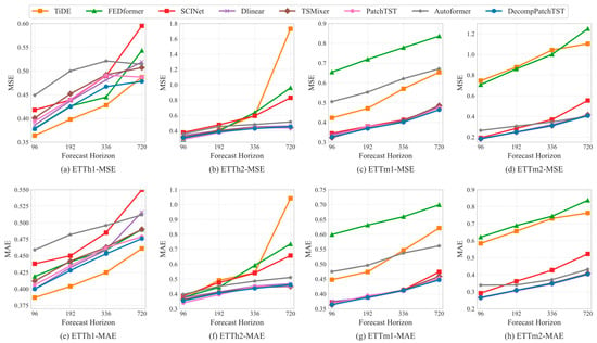
Table 3 presents the performance comparison results of the proposed model and baseline methods on the ETT datasets. To further observe the overall trend of error variation with increasing prediction length, Figure 2 shows the changes in MAE and MSE across different prediction lengths. Based on the presented data, this paper summarizes the following three key findings: (1) DecompPatchTST demonstrates stable performance across all datasets and forecasting horizons. As shown in Table 3 and Figure 2, although the prediction errors of all models increase as the forecasting horizon extends from 96 to 720 steps, the proposed method consistently maintains competitive error levels on the ETT benchmarks, particularly on ETTm1 and ETTm2, compared with representative baselines such as PatchTST and SCINet. Compared with transformer-based baselines that rely primarily on attention mechanisms for temporal representation learning, the proposed architecture benefits from the explicit modeling of long-term trend dynamics through the polynomial extrapolation module, which contributes to smoother error growth as the prediction horizon increases. These findings support the conclusion that the proposed model exhibits stable performance and smoother error growth. (2) Different models exhibit varying capabilities in modeling trend, seasonal, and noise components, while DecompPatchTST demonstrates more stable performance. MLP-based models like TiDE show significant error growth as prediction length increases, particularly on the hourly ETTh2, and also underperform on minute-level high-noise datasets. Transformer-based methods like FEDformer, while achieving strong short-term forecasts on highly seasonal data via frequency-domain modeling, exhibit more pronounced error increases on ETTm datasets with obvious trend changes and high noise levels. In contrast, our model exhibits more stable error growth across all four ETT datasets. Compared with models that directly encode the raw sequence, the decomposition structure explicitly separates trend and residual components, enabling the model to handle long-term evolution patterns and short-term fluctuations through different branches. (3) Overall errors on ETTm1 and ETTm2 are lower than those on ETTh1 and ETTh2, while DecompPatchTST demonstrates more prominent advantages in this scenario. As shown in Table 3, due to higher sampling frequencies, the load and temperature variations in ETTm1 and ETTm2 present more continuous trajectories with easier-to-capture short-term dynamics, resulting in significantly lower errors for most models. Under these conditions, the decomposition module in our model can more effectively extract trend and residual components. The polynomial extrapolation module achieves more stable fitting, while the residual branch can extract seasonal patterns and short-term fluctuations from local time patches. Consequently, the model demonstrates more significant performance advantages on ETTm datasets.

Figure 2. Performance visualization on the ETTh1, ETTh2, ETTm1 and ETTm2 datasets.

5.4.2. Robustness Analysis

To further evaluate the robustness of the proposed method for long-horizon forecasting, additional experiments were conducted on ETT datasets using five different random seeds (2019, 2020, 2021, 2022, and 2023) for the 336 and 720 prediction horizons. The mean and standard deviation of the MAE and MSE are reported in Table 4. To statistically assess whether the forecasting error increases significantly with longer horizons, paired t-tests were performed between the two horizons, and the corresponding p-values are also listed in Table 4. The results indicate that the forecasting error increases significantly when the horizon is extended from 336 to 720 steps, which is consistent with the inherent difficulty of long-term forecasting. Despite this increase, the standard deviations across random seeds remain relatively small, indicating stable performance under different random initializations. Larger deviations are observed on ETTh1 and ETTh2 at the 720-step horizon, which can be attributed to the increased uncertainty inherent in long-range forecasting for hourly datasets. These results demonstrate that DecompPatchTST maintains consistent predictive performance with controlled error growth across different experimental settings.

Table 4. Long-term forecasting results with different random seeds in DecompPatchTST.

Metric		336	720	p-Value
ETTh1	MSE	0.469 ± 0.004	0.489 ± 0.007	0.007 **
	MAE	0.454 ± 0.002	0.481 ± 0.004	0.000 ***
ETTh2	MSE	0.429 ± 0.004	0.444 ± 0.005	0.027 *
	MAE	0.438 ± 0.002	0.457 ± 0.003	0.002 **
ETTm1	MSE	0.403 ± 0.001	0.466 ± 0.002	0.000 ***
	MAE	0.411 ± 0.001	0.448 ± 0.001	0.000 ***
ETTm2	MSE	0.310 ± 0.003	0.408 ± 0.001	0.000 ***
	MAE	0.348 ± 0.002	0.405 ± 0.002	0.000 ***

* p-values from paired t-tests comparing performance at 336 and 720 prediction horizons. * p < 0.05, ** p < 0.01, *** p < 0.001.

Real-world time series are typically non-stationary, where statistical characteristics evolve over time. The proposed DecompPatchTST framework improves generalization under such conditions through structured modeling. Specifically, the decomposition module separates the input sequence into trend and residual components, reducing interference between long-term evolution and short-term fluctuations. The polynomial trend module models smooth long-term dynamics, while the PatchTST encoder module captures local temporal patterns via patch segmentation and attention. These components jointly enhance the robustness of the model when applied to time series with changing statistical properties.

5.5. Application Validation

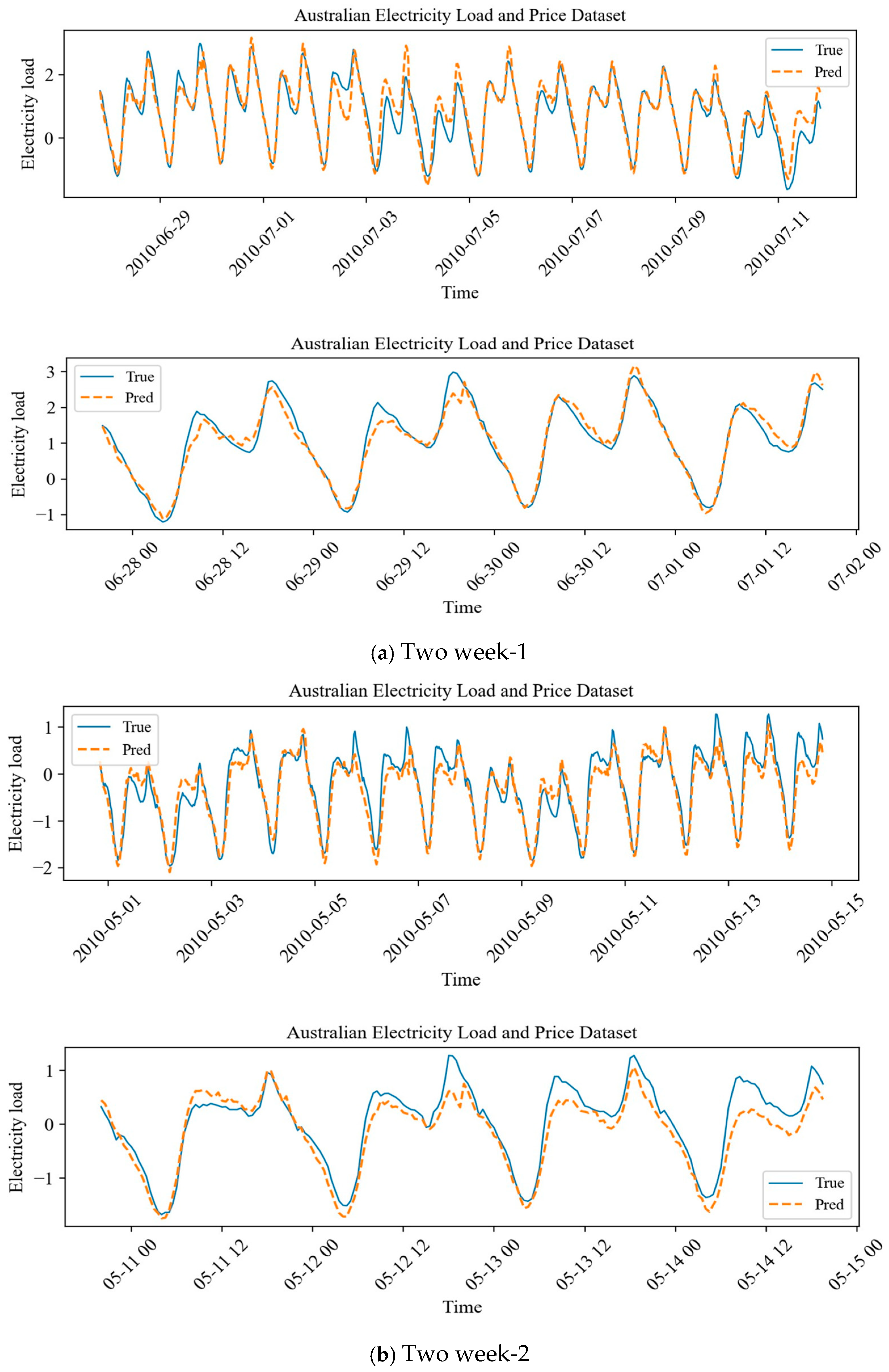
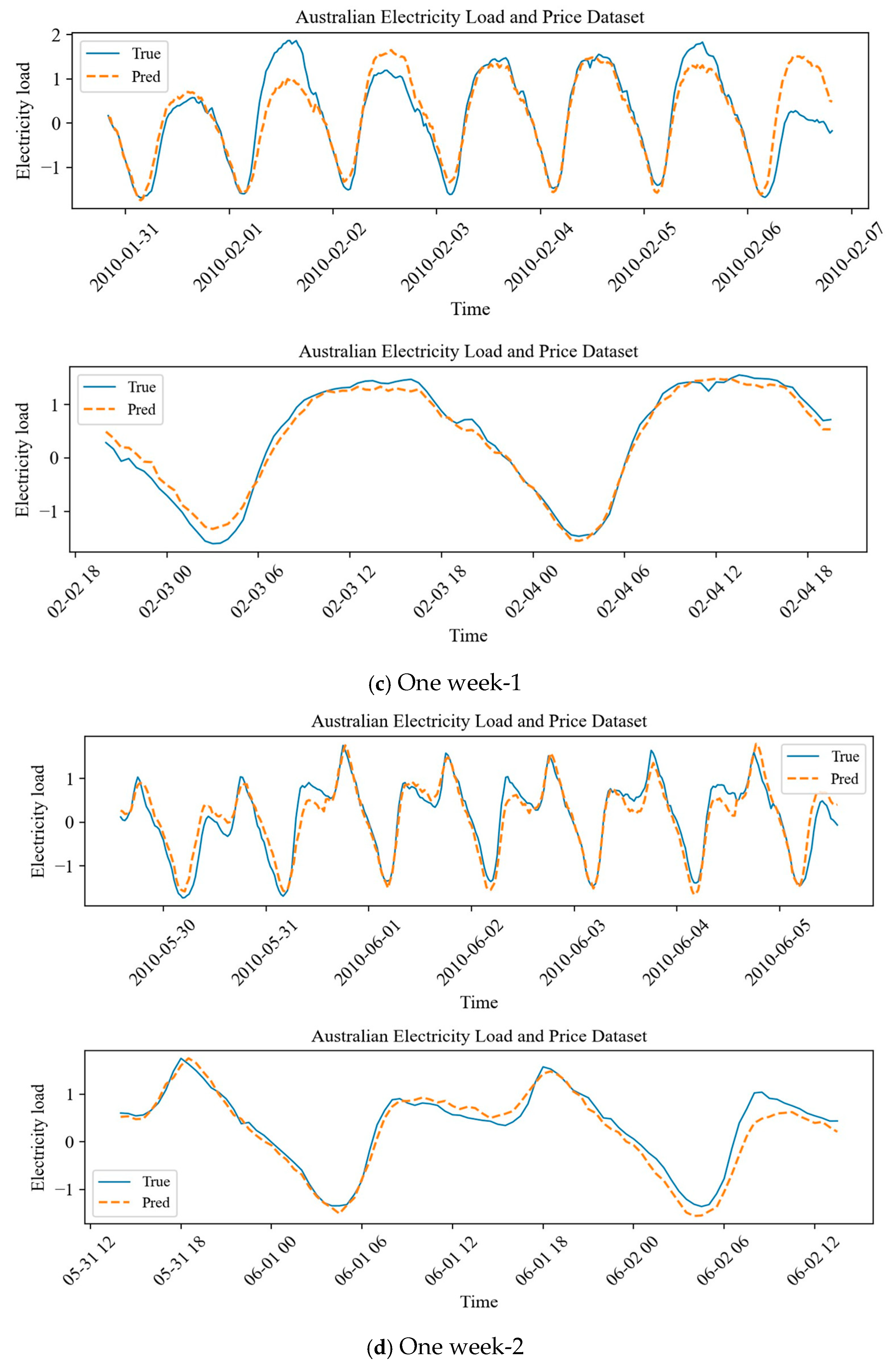
To verify the applicability of the DecompPatchTST model in real-world scenarios, a case study was conducted using the Australian electricity load and price dataset. This dataset contains six feature columns sampled at 30-minute intervals from January 2006 to January 2011. This experiment adopts the same multivariate forecasting setup, historical window length, and prediction window as used with the ETT datasets and maintains identical hyperparameters to ensure fair comparison. The data are split into training, validation, and test sets in a 6:2:2 ratio. For intuitive performance assessment, Figure 3 visualizes the model’s electricity load forecasts, with actual values in blue and predicted values in orange. This experiment uses a historical window of length 96 to predict the next 96 time steps. We take the prediction at the 96th step as the final forecast for that moment and obtain a complete forecast sequence corresponding to the actual series via a sliding window approach.

Figure 3. Visualization of forecasting performance on the Australian electricity load and price dataset.

Forecast results for one-week electricity load sequences from two different time periods are selected, along with corresponding two-day local magnified views. Additionally, two-week forecast plots from two different periods and their respective two-day local views are included to illustrate the weekly periodicity. The analysis reveals that: (1) Australian electricity load exhibits typical diurnal periodicity, characterized by a load increase in the early morning, maintaining high levels during the day, an evening peak, and a rapid decrease at night. On a weekly scale, a weekly periodicity is also present, with load generally higher on weekdays than on weekends. Different one-week sequences from various periods consistently reflect this pattern, and our model stably predicts the daily peaks and troughs while maintaining a periodic rhythm consistent with the actual series, demonstrating its effective modeling of the periodic component. (2) In the two-day magnified views, it can be observed that the real electricity load series during the early morning rise phase and the evening decline phase exhibits relatively smooth curves but still contains slight fluctuations. The DecompPatchTST model maintains good prediction accuracy even in these fine-grained regions, indicating that its residual modeling branch can effectively capture short-term fluctuations, while the trend branch can reliably capture the smooth changes in the series. (3) Moreover, the decomposed outputs of DecompPatchTST align with tangible phenomena in power systems: the trend component corresponds to the long-term base load, the seasonal component captures recurring daily or weekly cycles, and the noise component accounts for irregular short-term variations due to factors like weather shifts, user behavior or random outages. This mapping underscores the model’s interpretability and practical relevance for power management.

Overall, the DecompPatchTST effectively captures information at different scales in real electricity market data and provides credible forecast outputs, demonstrating its generalization capability to non-stationary time series with varying patterns and its application value in practical contexts such as power management.

5.6. Ablation Experiments

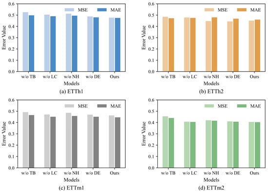
To evaluate the contribution of each core component in the DecompPatchTST, ablation experiments were conducted on four benchmark datasets using a prediction horizon of 720 steps. By removing or replacing key modules, four variants were constructed. The results are shown in Table 5.

Table 5. Ablation experiment on the DecompPatchTST structure.

Model	ETTh1		ETTh2		ETTm1		ETTm2
	MSE	MAE	MSE	MAE	MSE	MAE	MSE	MAE
w/o TB	0.527	0.499	0.486	0.473	0.493	0.467	0.456	0.441
w/o LC	0.505	0.491	0.480	0.476	0.472	0.452	0.408	0.406
w/o NH	0.514	0.496	0.448	0.481	0.487	0.459	0.421	0.417
w/o DE	0.489	0.481	0.445	0.469	0.471	0.452	0.411	0.408
DecompPatchTST (Ours)	0.478	0.476	0.452	0.461	0.464	0.447	0.406	0.404

Bold indicates the best performance.

The specific experimental designs are as follows: the w/o TB variant removes the trend modeling branch to evaluate its impact on overall performance; the w/o LC variant disables the coefficient learning module and uses fixed OLS coefficients to verify whether the trend extrapolation module requires adaptive learning capability; the w/o NH variant merges the dual prediction heads into a single prediction head to assess the advantage of decomposing the residual into noise and seasonal components for independent modeling; the w/o DE variant removes the time-series decomposition module, allowing both the trend and residual branches to directly use the original sequence as input.

Table 5 and Figure 4 present the results and corresponding visualizations, demonstrating the key contributions of each component to improving long-sequence forecasting performance.

Figure 4. Ablation analysis of the DecompPatchTST model.

As shown in Table 5 and Figure 4, all four ablation variants exhibit varying degrees of performance degradation. The w/o TB variant has the highest error, with MAE and MSE reaching 0.499 and 0.527 on the ETTh1 dataset. This is because the model relies solely on the residual branch to predict the series after trend removal while retaining the decomposition module, without explicitly modeling long-term trends. As a result, noticeable deviations in predicting the real series occur, leading to increased error. Compared with linear trend modeling approaches such as DLinear, the polynomial trend module in DecompPatchTST better captures nonlinear trend evolution, contributing to improved forecasting accuracy. The w/o NH variant follows, effectively demonstrating that splitting the residual branch into seasonal and noise components for separate prediction helps to reduce the interference of short-term disturbances and improves the model’s forecasting accuracy. The w/o LC variant, which uses fixed learning coefficients, can capture basic trends but cannot adaptively adjust the coefficients according to temporal variations in the series. This makes it difficult to fit the actual trend curvature in the prediction interval, resulting in relatively obvious errors. The w/o DE variant exhibits slightly higher errors than the complete model. Although this variant retains the trend and residual branches, it directly uses the original series as input, lacking the smooth trend component obtained via moving-average decomposition and the residual signal after trend removal. Therefore, its overall performance is slightly inferior to the complete model yet still better than the other variants. The results of these four ablation experiments confirm the effective contribution of each component to the model’s forecasting performance.

5.7. Parameter Sensitivity

To evaluate the impact of the moving-average kernel size, experiments were conducted on the ETTh1 dataset under prediction horizons of 96, 192, 336, and 720, with kernel sizes {13, 25, 51, 75}. The results in Table 6 show that, when the kernel size is set to 13, both MAE and MSE are consistently higher across all horizons. This indicates that insufficient smoothing allows high-frequency fluctuations to remain in the extracted trend component, which slightly affects the stability of polynomial extrapolation. When the kernel size increases to 25 and above, forecasting performance becomes stable, and the differences among 25, 51, and 75 are marginal. This suggests that, once the primary low-frequency structure of the series is effectively captured, further enlarging the smoothing window does not significantly alter the trend representation. Notably, under hourly sampling, a kernel size of 25 approximately corresponds to one-day smoothing, which aligns with the intrinsic daily periodicity of electricity load data. Considering both forecasting stability and practical interpretability, kernel size 25 is adopted as the default configuration.

Table 6. Parameter sensitivity experiment on the DecompPatchTST structure on ETTh1 dataset.

Metric	13		25		51		75
	MSE	MAE	MSE	MAE	MSE	MAE	MSE	MAE
96	0.381	0.400	0.378	0.400	0.376	0.399	0.375	0.399
192	0.446	0.437	0.425	0.428	0.422	0.429	0.426	0.430
336	0.494	0.468	0.467	0.453	0.465	0.453	0.463	0.452
720	0.528	0.503	0.478	0.476	0.469	0.467	0.468	0.469

5.8. Complexity Analysis

To evaluate the computational efficiency of DecompPatchTST, we compare it with two representative baselines: PatchTST and DLinear. PatchTST is selected for sharing a patch-based transformer encoder architecture with our model and achieving competitive forecasting accuracy, as detailed in Table 3. DLinear is chosen as a lightweight decomposition-based linear model with high computational efficiency. Experiments are conducted on the ETTh1 dataset with a fixed lookback length of 96 and four prediction horizons. Theoretically, the complexity of our model, similar to PatchTST, is dominated by patch attention, while DLinear scales linearly with input length. Table 7 reports the parameter counts and FLOPs, which measure temporal and spatial complexity, respectively. As shown in Table 7, DecompPatchTST reduces parameters relative to PatchTST at the cost of higher FLOPs. DLinear achieves the lowest complexity in both dimensions yet underperforms our model in accuracy. These results indicate that accuracy gains typically come with increased spatiotemporal complexity, motivating future work to reduce complexity while preserving predictive performance.

Table 7. Comparison of the spatial–temporal complexity.

Models	DecompPatchTST		PatchTST		DLinear
Metric	Params (M)	FLOPS (G)	Params (M)	FLOPS (G)	Params (M)	FLOPS (M)
96	3.27	15.70	3.76	8.63	0.02	4.15
192	3.37	15.74	4.35	8.76	0.04	8.28
336	3.52	15.81	5.24	8.96	0.07	14.47
720	3.91	15.99	7.60	9.49	0.14	30.98

6. Conclusions

Focusing on prevalent challenges in long-term TSF, including trend evolution, periodic patterns, and noise interference, this paper proposes DecompPatchTST, a forecasting model incorporating a decomposition methodology. The model employs a moving average to decompose the original series into trend and residual components, thereby disentangling the broken symmetry. It utilizes a learnable polynomial extrapolation module to predict long-term trends and a patch-based transformer encoder with dual prediction heads to model seasonal patterns and noise. The final additive aggregation completes the symmetric reconstruction. The experimental results on four ETT benchmark datasets demonstrate that the model achieves more stable performance across different prediction lengths, particularly in long-term forecasting tasks with 720 steps. The ablation results further indicate that each component contributes significantly to the overall performance. Additionally, a visualization analysis on real Australian electricity load and price datasets verifies the model’s applicability in practical scenarios. The model effectively captures intraday and weekly periodicities and maintains robustness against short-term disturbances, thereby providing reliable forecasts. Future work will explore the use of state-space models such as Mamba to replace the transformer encoder in the residual branch, thereby improving model efficiency while preserving predictive performance.

References

- Nafea, A.A.; Alawi, O.A.; Doost, Z.H.; AlAni, M.M.; Ahmadullah, A.B.; Deo, R.C.; Yaseen, Z.M. Electricity load and price forecasting in Spain: A hybrid deep learning framework leveraging temporal and seasonal dynamics. Expert Syst. Appl. 2026, 299, 130123. [Google Scholar] [CrossRef] [Scilit]
- Zhao, Y.; Zhang, W.; Liu, X. Grid search with a weighted error function: Hyper-parameter optimization for financial time series forecasting. Appl. Soft Comput. 2024, 154, 111362. [Google Scholar] [CrossRef] [Scilit]
- Yang, M.; Jiang, Y.; Zhang, W.; Li, Y.; Su, X. Short-term interval prediction strategy of photovoltaic power based on meteorological reconstruction with spatiotemporal correlation and multi-factor interval constraints. Renew. Energy 2024, 237, 121834. [Google Scholar] [CrossRef] [Scilit]
- Kong, X.; Chen, Z.; Liu, W.; Ning, K.; Zhang, L.; Marier, S.M.; Liu, Y.; Chen, Y.; Xia, F. Deep learning for time series forecasting: A survey. Int. J. Mach. Learn. Cybern. 2025, 16, 5079–5112. [Google Scholar] [CrossRef] [Scilit]
- Tarmanini, C.; Sarma, N.; Gezegin, C.; Ozgonenel, O. Short term load forecasting based on ARIMA and ANN approaches. Energy Rep. 2023, 9, 550–557. [Google Scholar] [CrossRef] [Scilit]
- Düker, M.-C.; Matteson, D.S.; Tsay, R.S.; Wilms, I. Vector AutoRegressive moving average models: A review. WIREs Comput. Stat. 2025, 17, e70009. [Google Scholar] [CrossRef] [Scilit]
- Mienye, I.D.; Swart, T.G.; Obaido, G. Recurrent neural networks: A comprehensive review of architectures, variants, and applications. Information 2024, 15, 517. [Google Scholar] [CrossRef] [Scilit]
- Krichen, M.; Mihoub, A. Long short-term memory networks: A comprehensive survey. AI 2025, 6, 215. [Google Scholar] [CrossRef] [Scilit]
- Dey, R.; Salem, F.M. Gate-variants of gated recurrent unit (GRU) neural networks. In Proceedings of the 2017 IEEE 60th International Midwest Symposium on Circuits and Systems (MWSCAS), Boston, MA, USA, 6–9 August 2017; IEEE: Piscataway, NJ, USA, 2017; pp. 1597–1600. [Google Scholar] [CrossRef] [Scilit]
- Lecun, Y.; Bottou, L.; Bengio, Y.; Haffner, P. Gradient-based learning applied to document recognition. Proc. IEEE 1998, 86, 2278–2324. [Google Scholar] [CrossRef] [Scilit]
- Vaswani, A.; Shazeer, N.; Parmar, N.; Uszkoreit, J.; Jones, L.; Gomez, A.N.; Kaiser, Ł.U.; Polosukhin, I. Attention is all you need. In Advances in Neural Information Processing Systems; Curran Associates, Inc.: Red Hook, NY, USA, 2017; Volume 30. [Google Scholar] [CrossRef] [Scilit]
- Liu, Y.; Hu, T.; Zhang, H.; Wu, H.; Wang, S.; Ma, L.; Long, M. iTransformer: Inverted Transformers Are Effective for Time Series Forecasting. arXiv 2023, arXiv:2310.06625. [Google Scholar]
- Zhou, T.; Ma, Z.; Wen, Q.; Wang, X.; Sun, L.; Jin, R. FEDformer: Frequency enhanced decomposed transformer for long-term series forecasting. In Proceedings of the Proceedings of the 39th International Conference on Machine Learning(ICML), Baltimore, MD, USA, 28 June 2022; pp. 27268–27286. [Google Scholar] [CrossRef] [Scilit]
- Wu, H.; Hu, T.; Liu, Y.; Zhou, H.; Wang, J.; Long, M. Timesnet: Temporal 2d-variation modeling for general time series analysis. arXiv 2022, arXiv:2210.02186. [Google Scholar]
- Zhang, Y.; Yan, J. Crossformer: Transformer utilizing cross-dimension dependency for multivariate time series forecasting. In Proceedings of the The Eleventh International Conference on Learning Representations (ICLR), Kigali, Rwanda, 23 January 2023. [Google Scholar]
- Ekambaram, V.; Jati, A.; Nguyen, N.; Sinthong, P.; Kalagnanam, J. TSMixer: Lightweight MLP-mixer model for multivariate time series forecasting. In Proceedings of the 29th ACM SIGKDD Conference on Knowledge Discovery and Data Mining; ACM: Long Beach, CA, USA, 6 August 2023; pp. 459–469. [Google Scholar] [CrossRef] [Scilit]
- Gu, A.; Dao, T. Mamba: Linear-time sequence modeling with selective state spaces. arXiv 2023, arXiv:2312.00752. [Google Scholar] [CrossRef] [Scilit]
- Ansari, A.F.; Stella, L.; Turkmen, C.; Zhang, X.; Mercado, P.; Shen, H.; Shchur, O.; Rangapuram, S.S.; Arango, S.P.; Kapoor, S.; et al. Chronos: Learning the language of time series. arXiv 2024, arXiv:2403.07815. [Google Scholar] [CrossRef] [Scilit]
- Jin, M.; Wang, S.; Ma, L.; Chu, Z.; Zhang, J.Y.; Shi, X.; Chen, P.-Y.; Liang, Y.; Li, Y.-F.; Pan, S.; et al. Time-LLM: Time series forecasting by reprogramming large language models. arXiv 2024, arXiv:2310.01728. [Google Scholar] [CrossRef] [Scilit]
- Trull, O.; García-Díaz, J.C.; Peiró-Signes, A. Multiple seasonal STL decomposition with discrete-interval moving seasonali-ties. Appl. Math. Comput. 2022, 433, 127398. [Google Scholar] [CrossRef] [Scilit]
- Zeng, A.; Chen, M.; Zhang, L.; Xu, Q. Are transformers effective for time series forecasting? In Proceedings of the Thirty-Seventh AAAI Conference on Artificial Intelligence (AAAI-23), Washington, DC, USA, 7–14 February 2023; Volume 37, pp. 11121–11128. [Google Scholar] [CrossRef] [Scilit]
- Nie, Y.; Nguyen, N.H.; Sinthong, P.; Kalagnanam, J. A time series is worth 64 words: Long-term forecasting with transformers. In Proceedings of the The Eleventh International Conference on Learning Representations (ICLR), Kigali, Rwanda, 1–5 May 2023. [Google Scholar] [CrossRef] [Scilit]
- ArunKumar, K.E.; Kalaga, D.V.; Mohan Sai Kumar, C.; Kawaji, M.; Brenza, T.M. Comparative analysis of gated recurrent units (GRU), long short-term memory (LSTM) cells, autoregressive integrated moving average (ARIMA), seasonal autoregressive integrated moving average (SARIMA) for forecasting COVID-19 trends. Alex. Eng. J. 2022, 61, 7585–7603. [Google Scholar] [CrossRef] [Scilit]
- Li, X.; Yuan, J. DeepVARwT: Deep learning for a VAR model with trend. arXiv 2022, arXiv:2209.10587. [Google Scholar] [CrossRef] [Scilit]
- Wu, J.; Wang, Y.-G.; Zhang, H. Augmented support vector regression with an autoregressive process via an iterative procedure. Appl. Soft Comput. 2024, 158, 111549. [Google Scholar] [CrossRef] [Scilit]
- Ge, J.; Zhao, L.; Yu, Z.; Liu, H.; Zhang, L.; Gong, X.; Sun, H. Prediction of greenhouse tomato crop evapotranspiration using XGBoost machine learning model. Plants 2022, 11, 1923. [Google Scholar] [CrossRef] [Scilit]
- Ben Taieb, S.; Bontempi, G. Recursive multi-step time series forecasting by perturbing data. In Proceedings of the 2011 IEEE 11th International Conference on Data Mining, Vancouver, BC, Canada, 11–14 December 2011; IEEE: Piscataway, NJ, USA, 2011; pp. 695–704. [Google Scholar] [CrossRef] [Scilit]
- Ben Taieb, S.; Bontempi, G.; Atiya, A.F.; Sorjamaa, A. A review and comparison of strategies for multi-step ahead time series forecasting based on the NN5 forecasting competition. Expert Syst. Appl. 2012, 39, 7067–7083. [Google Scholar] [CrossRef] [Scilit]
- Chung, J.; Gulcehre, C.; Cho, K.; Bengio, Y. Empirical evaluation of gated recurrent neural networks on sequence modeling. arXiv 2014, arXiv:1412.3555. [Google Scholar] [CrossRef] [Scilit]
- LIU, M.; Zeng, A.; Chen, M.; Xu, Z.; LAI, Q.; Ma, L.; Xu, Q. SCINet: Time series modeling and forecasting with sample convolution and interaction. In Advances in Neural Information Processing Systems; Curran Associates, Inc.: Red Hook, NY, USA, 2022; Volume 35, pp. 5816–5828. [Google Scholar] [CrossRef] [Scilit]
- Wang, P.; Chen, P.; Yuan, Y.; Liu, D.; Huang, Z.; Hou, X.; Cottrell, G. Understanding convolution for semantic segmentation. In Proceedings of the 2018 IEEE Winter Conference on Applications of Computer Vision (WACV), Lake Tahoe, NV, USA, 12–15 March 2018; pp. 1451–1460. [Google Scholar] [CrossRef] [Scilit]
- Yu, F.; Koltun, V. Multi-scale context aggregation by dilated convolutions. In Proceedings of the International Conference on Learning Representations (ICLR), San Juan, Puerto Rico, 2–4 May 2016. [Google Scholar] [CrossRef] [Scilit]
- Lim, B.; Zohren, S. Time series forecasting with deep learning: A survey. Philos. Trans. R. Soc. A 2021, 379, 20200209. [Google Scholar] [CrossRef] [Scilit] [PubMed]
- Xu, X.; Ren, W. A hybrid model based on a two-layer decomposition approach and an optimized neural network for chaotic time series prediction. Symmetry 2019, 11, 610. [Google Scholar] [CrossRef] [Scilit]
- Wu, H.; Xu, J.; Wang, J.; Long, M. Autoformer: Decomposition transformers with auto-correlation for long-term series forecasting. In Proceedings of the Advances in Neural Information Processing Systems; Curran Associates, Inc.: Red Hook, NY USA, 2021; Volume 34, pp. 22419–22430. [Google Scholar] [CrossRef] [Scilit]
- Woo, G.; Liu, C.; Sahoo, D.; Kumar, A.; Hoi, S. Learning deep time-index models for time series forecasting. In Proceedings of the Proceedings of the 40th International Conference on Machine Learning, Honolulu, HI, USA, 23–29 July 2023; Volume 203, pp. 37217–37237. [Google Scholar] [CrossRef] [Scilit]
- Bryan, M.J.; Schwock, F.; Yazdan-Shahmorad, A.; Rao, R.P.N. Temporal basis function models for closed-loop neural stimulation. J. Neural Eng. 2025, 22, 056012. [Google Scholar] [CrossRef] [Scilit]
- Shen, X.; Meinshausen, N. Engression: Extrapolation through the lens of distributional regression. arXiv 2023, arXiv:2307.00835. [Google Scholar] [CrossRef] [Scilit]
- Wang, Z.; Kong, F.; Feng, S.; Wang, M.; Yang, X.; Zhao, H.; Wang, D.; Zhang, Y. Is mamba effective for time series forecasting? Neurocomputing 2025, 619, 129178. [Google Scholar] [CrossRef] [Scilit]
- Toner, W.; Darlow, L. An analysis of linear time series forecasting models. arXiv 2024, arXiv:2403.14587. [Google Scholar] [CrossRef] [Scilit]
- Han, L.; Chen, X.-Y.; Ye, H.-J.; Zhan, D.-C. SOFTS: Efficient multivariate time series forecasting with series-core fusion. Adv. Neural Inf. Process. Syst. 2024, 37, 64145–64175. [Google Scholar] [CrossRef] [Scilit]
- Fan, J.; Shen, Y. StockMixer: A simple yet strong MLP-based architecture for stock price forecasting. Assoc. Adv. Artif. Intell. 2024, 38, 8389–8397. [Google Scholar] [CrossRef] [Scilit]
- Das, A.; Kong, W.; Leach, A.; Mathur, S.; Sen, R.; Yu, R. Long-term forecasting with TiDE: Time-series dense encoder. arXiv 2023, arXiv:2304.08424. [Google Scholar]
- Loshchilov, I.; Hutter, F. Decoupled weight decay regularization. In Proceedings of the International Conference on Learning Representations (ICLR), New Orleans, LA, USA, 6–9 May 2019; Volume 97, pp. 4061–4079. [Google Scholar] [CrossRef] [Scilit]
- Long, Y.; Qin, X. A multivariate time series prediction model based on the KAN network. Sci. Rep. 2025, 15, 23621. [Google Scholar] [CrossRef] [Scilit] [PubMed]
Disclaimer/Publisher’s Note: The statements, opinions and data contained in all publications are solely those of the individual author(s) and contributor(s) and not of MDPI and/or the editor(s). MDPI and/or the editor(s) disclaim responsibility for any injury to people or property resulting from any ideas, methods, instructions or products referred to in the content. |
© 2026 by the authors. Licensee MDPI, Basel, Switzerland. This article is an open access article distributed under the terms and conditions of the Creative Commons Attribution (CC BY) license.