A Decomposition-Driven Hybrid Approach to Forecasting Oil Market Dynamics

Abstract

Modeling nonstationary time series in financial and energy markets remains challenging due to nonlinear dynamics, volatility clustering, and frequent regime shifts that distort the underlying probabilistic structure of the data. This study introduces a novel probabilistic–statistical decomposition framework, termed Robust Adaptive Decomposition (RAD), designed to preserve probabilistic symmetry between deterministic and stochastic components. In this context, symmetry refers to maintaining statistical balance—particularly in the means, variances, and distributional structures—between the extracted modes and the residual series, thereby preventing artificial bias or variance distortion during decomposition. The RAD framework adaptively determines the optimal number of modes needed to effectively separate short-term fluctuations from long-term structural movements. Unlike conventional techniques, such as Empirical Mode Decomposition (EMD), Ensemble EMD (EEMD), and CEEMDAN, the proposed method incorporates a robustness mechanism that mitigates mode mixing and reduces distortions induced by extreme shocks and regime transitions. The empirical evaluation is conducted on six oil-related energy commodities—Brent crude oil, kerosene, propane, sulfur diesel, heating oil, and gasoline—whose price dynamics exhibit pronounced nonlinearity and structural volatility. When integrated with ARIMA forecasting models, the RAD-based framework consistently outperforms benchmark decomposition approaches. Across all datasets, RAD–ARIMA achieves reductions of approximately 65–90% in MAE, 60–85% in RMSE, and up to 95% in MAPE relative to CEEMDAN-based models. These results demonstrate that RAD provides a mathematically rigorous and computationally efficient preprocessing mechanism that preserves statistical equilibrium while effectively disentangling deterministic structures from stochastic noise. Beyond oil markets, the framework offers broad applicability in econometric modeling, financial forecasting, and risk management, contributing to probability- and statistics-driven symmetry analysis in complex dynamic systems.

1. Introduction

Accurate forecasting of energy and financial commodity prices remains a central problem in mathematical finance, econometrics, and applied probability [1]. Energy commodities such as crude oil, kerosene, propane, and heating oil play a critical role in global economic activity, as their price fluctuations influence energy security, portfolio allocation, hedging strategies, and systemic financial stability. Reliable forecasting, therefore, supports both microeconomic decision-making and macroeconomic policy design, risk management, and regulatory planning [2,3,4,5].

From a statistical standpoint, energy price series exhibit volatility clustering, regime shifts, nonlinear dependence structures, and pronounced nonstationarity [6,7,8]. These characteristics challenge classical linear econometric models, which rely on restrictive distributional and stationarity assumptions. Early econometric approaches, including small-scale structural models and nonlinear regression frameworks [9,10], laid the foundation for systematic oil price forecasting. Subsequently, ARIMA and GARCH models became dominant tools, capturing temporal dependence and conditional heteroskedasticity in crude oil markets [11,12,13]. While ARIMA effectively models linear lag structures and GARCH accounts for time-varying volatility, their performance deteriorates in the presence of strong nonlinearities and structural breaks.

In parallel with advances in classical econometrics, machine learning (ML) and deep learning models have been increasingly applied to energy price forecasting. Methods such as support vector regression [14], Gaussian process regression [15], random forests [16,17], boosting algorithms [18], ensemble learning [19,20,21], and long short-term memory (LSTM) networks [22,23] have been employed to capture nonlinear patterns in crude oil and related energy markets. Hybrid deep-learning approaches combining decomposition with neural architectures further enhance predictive flexibility [24,25,26]. Despite their modeling power, purely data-driven approaches may fail to fully exploit structural information embedded in raw time-series data and often suffer from reduced interpretability and unstable performance under regime shifts [27,28]. Empirical comparisons also indicate that traditional statistical models can outperform advanced ML algorithms under certain conditions [29,30,31], underscoring the importance of robust statistical structure in forecasting design.

Collectively, the literature reveals three consistent observations: (i) energy price series are inherently nonlinear, nonstationary, and heteroskedastic; (ii) decomposition–reconstruction strategies improve forecasting by isolating structural components; and (iii) no single modeling paradigm consistently dominates across market regimes. These insights motivate the development of a symmetry-aware, statistically robust decomposition framework that stabilizes noise separation while preserving the probabilistic structure of the original series.

In response, this study proposes a novel Robust Adaptive Decomposition (RAD) framework. RAD is formulated as a symmetry-preserving, data-adaptive filtering procedure that explicitly separates deterministic components from stochastic fluctuations. Unlike conventional EMD-based approaches, RAD directly estimates the degree of noise separation from the data, without relying on predefined rules for IMF extraction. The framework incorporates a distance-based adaptive weighting mechanism, enabling robust residual construction under volatility shocks and regime transitions. Boundary stabilization through weighted endpoint averaging further reduces edge effects and enhances numerical stability.

The proposed RAD framework is integrated with both ARIMA and LSTM forecasting models to evaluate its effectiveness across multiple oil-related energy commodities. Performance is assessed using comprehensive statistical accuracy measures to ensure robust comparative evaluation. The main contributions of this study are summarized as follows:

• A symmetry-preserving and robust adaptive decomposition technique is developed to extract informative residual signals from nonlinear and nonstationary energy price series.
• A decomposition-based filtering mechanism is introduced to selectively eliminate noisy intrinsic components while retaining essential structural information.
• A distance-based adaptive weighting scheme is formulated to mitigate outlier influence and stabilize residual estimation under extreme volatility.
• An adaptive stopping strategy is designed to determine the optimal degree of noise separation, reducing computational complexity while improving statistical consistency.
• The RAD framework enhances compatibility with both econometric and machine-learning forecasting models, thereby improving predictive accuracy and model interpretability.

The remainder of the paper is organized as follows. Section 2 reviews the relevant literature and positions the proposed framework within existing studies on probabilistic forecasting and financial time-series modeling. Section 3 presents the mathematical formulation of RAD and its integration with forecasting models. Section 4 provides empirical results and comparative analysis. Finally, Section 5 concludes the paper and outlines future research directions in probabilistic time-series modeling and financial econometrics.

2. Related Work

Decomposition-based hybrid methodologies have gained substantial prominence in energy price forecasting [32,33,34,35,36]. Techniques such as Empirical Mode Decomposition (EMD), Ensemble EMD (EEMD), and Complete Ensemble EMD with Adaptive Noise (CEEMDAN) have been widely adopted to separate time series into intrinsic mode functions (IMFs) prior to forecasting [37,38,39,40]. Hybrid frameworks integrating decomposition with ARIMA, sparse Bayesian learning, or other predictive models have demonstrated improvements in forecasting accuracy [41,42,43,44]. Nevertheless, these methods often suffer from mode mixing, instability under extreme volatility, and sensitivity to noise contamination, limiting their statistical interpretability and robustness [40,45,46].

Huang et al. [47] introduced Empirical Mode Decomposition (EMD), a data-driven method that decomposes complex signals into intrinsic mode functions representing mono-components with well-defined instantaneous frequencies. However, EMD is prone to mode-mixing issues. To address this limitation, Ensemble Empirical Mode Decomposition (EEMD) was proposed as a noise-assisted technique [48]. By injecting Gaussian white noise into the original signal and averaging the resulting IMFs across realizations, EEMD mitigates mode mixing but introduces residual noise and inconsistencies in the number of extracted modes. Complementary EEMD (CEEMD) was later introduced by Jia-Rong Yeh et al. [49,50] using paired positive and negative noise realizations to improve reconstruction accuracy. Subsequently, Complete Ensemble Empirical Mode Decomposition with Adaptive Noise (CEEMDAN) was developed by Torres et al. [51,52,53,54], resolving reconstruction and mode-number inconsistencies. Despite these improvements, CEEMDAN may generate spurious modes during early decomposition stages [55,56,57].

Variational Mode Decomposition (VMD) offers an alternative non-recursive decomposition framework in which band-limited modes are estimated synchronously with adaptive center frequencies [58,59]. VMD has demonstrated advantages in tone separation and noise robustness [60]; however, it requires pre-specification of the number of modes and bandwidth parameters [61,62,63], making its performance sensitive to user-defined settings. Singular Spectrum Analysis (SSA) has also been widely applied for univariate decomposition and forecasting [64,65]. Although effective in certain settings, SSA depends critically on window-length selection, limiting its adaptability to structural changes and affecting forecasting stability. Thus, existing decomposition techniques rely heavily on parameter selection, noise injection strategies, or recursive sifting procedures. These limitations motivate the development of Robust Adaptive Decomposition (RAD), a parameter-free and symmetry-preserving framework designed to stabilize noise separation while maintaining statistical consistency. Unlike prior methods, RAD determines the degree of decomposition adaptively from the data itself, avoiding arbitrary parameter specification and reducing the risk of spurious component generation.

On the other hand, recent advances in financial machine learning have emphasized the importance of modeling cross-commodity and cross-asset dependencies to enhance forecasting performance. Multivariate frameworks such as vector autoregressive (VAR) models, multi-target regression approaches, and graph neural networks for financial time series explicitly capture inter-series correlations and shared market dynamics. Empirical evidence suggests that exploiting cross-asset information can significantly improve predictive accuracy in correlated markets [66,67]. However, the present study focuses on a univariate decomposition framework. The proposed RAD method is formulated for single-series analysis and aims to preserve probabilistic symmetry between deterministic and stochastic components within each commodity series. Extending RAD to a multivariate setting that incorporates cross-commodity dependencies remains an important direction for future research.

3. Methodology

This section presents the proposed RAD framework for analyzing nonlinear and nonstationary financial time series. RAD is formulated as a probabilistic-statistical decomposition operator that extracts informative intrinsic components while preserving symmetry between deterministic structures and stochastic fluctuations. Unlike conventional adaptive decomposition techniques such as Empirical Mode Decomposition (EMD), Ensemble EMD (EEMD), and CEEMDAN—RAD is grounded in robust statistical estimation and spline-based functional approximation, yielding decompositions that are stable under heavy-tailed distributions, volatility clustering, and regime shifts.

Let $X=\{X_1,X_2,\dots ,X_N\}$, $X_i\in \mathbb{R}$, denote a univariate discrete time series of length N, such as logarithmic returns of an energy commodity price. The objective of RAD is to decompose X into intrinsic oscillatory modes and a residual component while preserving probabilistic balance and structural symmetry.

• Robust Location and Scale Estimation:
  To ensure resistance against outliers and heavy tails, RAD employs robust estimators:

  $$m_X=median\left\{X_i\right\},\mathrm{MAD}=median\left\{\right|X_i-m_X\left|\right\}.$$
  These estimators possess a breakdown point of 50%, making them suitable for asymmetric financial data.
• Robust Symmetry-Aware Weighting:
  Each observation is standardized:

  $$Z_i={\displaystyle \frac{X_i-m_X}{\mathrm{MAD}}},i=1,\dots ,N.$$
  To attenuate extreme deviations, robustness weights are defined as

  $$W_i={\displaystyle \frac{1}{1+|Z_i|}}.$$
  This construction ensures symmetric treatment of positive and negative deviations while reducing the influence of outliers.
• Local Weighted Mean Construction:
  For each adjacent pair, a local weighted mean is defined as

  $${\mu }_i={\displaystyle \frac{W_i{X}_i+W_{i+1}{X}_{i+1}}{W_i+W_{i+1}}},i=1,\dots ,N-1.$$
• Spline-Based Functional Approximation:
  The sequence $\left\{{\mu }_i\right\}$ is extended to length N via symmetric boundary extension, forming

  $${\tilde{\mu }}_1,{\mu }_1,\dots ,{\mu }_{N-1},{\tilde{\mu }}_N.$$
  A cubic spline $S\left(t\right)$ is constructed over intervals $[t_i,t_{i+1}]$:

  $$S_i\left(t\right)=a_i+b_i(t-t_i)+c_i{(t-t_i)}^2+d_i{(t-t_i)}^3,t\in [t_i,t_{i+1}],$$

  with coefficients determined by enforcing continuity of $S\left(t\right)$ and its first two derivatives.
  The first residual component is then

  $$R_i^{\left(1\right)}=X_i-S\left(t_i\right),i=1,\dots ,N.$$
• Extraction of Intrinsic Mode Functions (IMFs):
  The first IMF is defined as

  $${\mathrm{IMF}}_1=X-R^{\left(1\right)},$$

  capturing high-frequency oscillatory behavior.
• Iterative Refinement and Stopping Criterion:
  The procedure is iteratively applied:

  $$X^{\left(j\right)}=R^{(j-1)},j\ge 2,$$

  $${\mathrm{IMF}}_j=X^{(j-1)}-R^{\left(j\right)}.$$
  The stopping rule is correlation-based:

  $$\rho ({\mathrm{IMF}}_k,X)<\rho ({\mathrm{IMF}}_{k-1},X),$$

  where $\rho (·)$ denotes the Pearson correlation with the original series.

The final decomposition is

$$X=\sum _{j=1}^K{\mathrm{IMF}}_j+R^{\left(K\right)},$$

where K is determined endogenously by the stopping criterion.

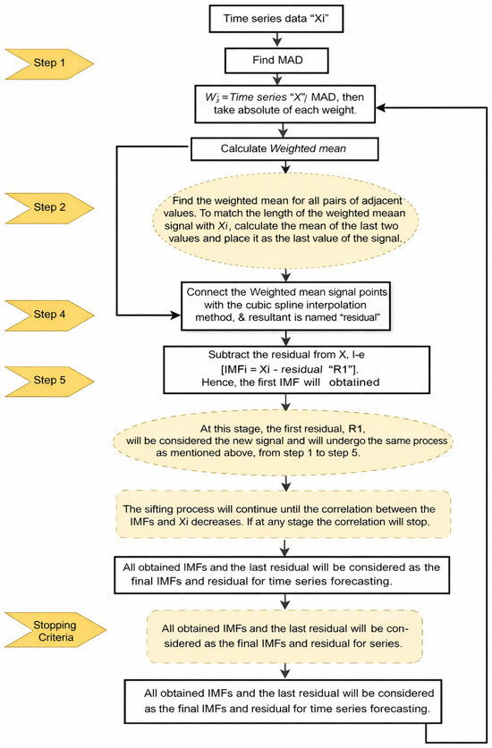
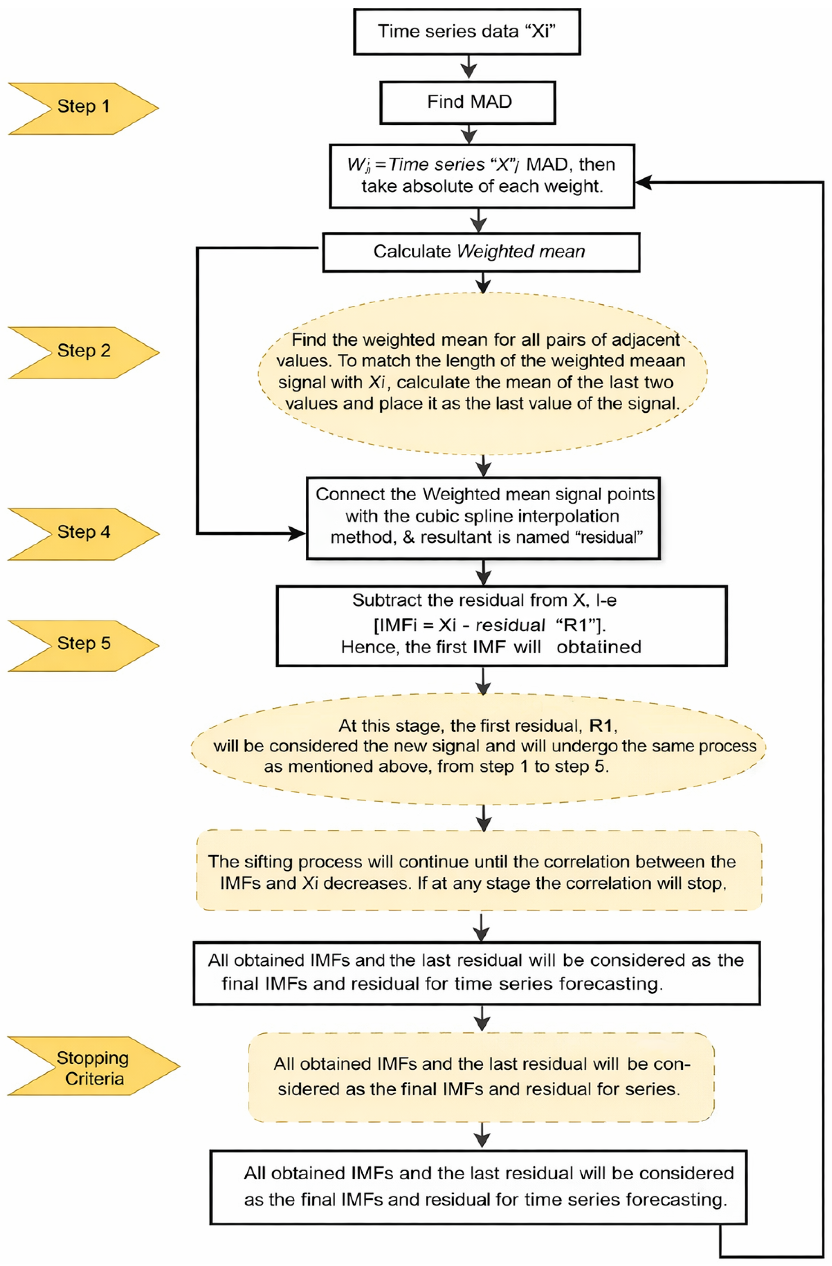
Algorithmically, the RAD is very different from Empirical Mode Decomposition (EMD) and its variants, EEMD and CEEMDAN. The EMD family of algorithms is clearly guided by two conditions for the intrinsic mode function (IMF): symmetry of local extrema and a zero-mean envelope. The EMD family of algorithms requires iterative sifting to enforce these two conditions. In contrast, the RAD algorithm does not attempt to enforce these IMF conditions and does not require local extrema, envelope interpolation, or sifting. The RAD algorithm primarily removes micro-scale oscillations, which can be viewed as noise, while preserving the deterministic component of the original signal. RAD also employs techniques such as cubic spline interpolation, weighted local means, and a correlation-based stopping function, all implemented in a fully generalized, data-adaptive fashion. The approach automatically identifies the number of modes for each time series based on the correlation pattern between the residual and the extracted components. The weighted local means are computed from consecutive points in the data, which capture local behavior; RAD then assumes that the residual signal corresponds to the long-term signal, excluding microscale fluctuations. The cubic spline interpolation extends the N-1 local means into a vector of length N to ensure smooth reconstruction of the residual while preserving the original series structure. With respect to the stopping criterion, RAD monitors the correlation between the current residual and the decomposed component at each iteration, and the decomposition procedure terminates when this correlation fails to decrease. Small oscillations due to noise are addressed by computing correlations within a sliding window or by considering the final minimum correlation point, thereby making the process more stable without requiring user-defined thresholds. Notably, RAD has been implemented in an R library [68], enabling reproducible application across datasets. Overall, these considerations ensure that the RAD algorithm automatically adjusts to different time series, distinguishing stochastic short-term oscillations from deterministic long-term components. Finally, a schematic overview of the RAD procedure is illustrated in Figure 1.

Figure 1. Flowchart of the proposed Robust Adaptive Decomposition (RAD) technique.

The main goal of the proposed RAD framework is to establish a clear and structure-preserving distinction between short-term and long-term variability in highly volatile time series, such as oil prices. In order to attain this objective, proposed a weighting mechanism and employed the resulting weights in a formulation of the mean, which is defined as the residual. The proposed weighting mechanism was designed to be robust to outliers, given that oil prices exhibit high volatility and abrupt price changes. In fact, traditional mean-based methods are highly susceptible to outliers and may compromise the decomposition process. However, the proposed weighted-mean approach reduces the influence of outliers and thus preserves the original signal structure. It is understood that each individual technique used within the framework of the proposed method, such as weighted mean, cubic spline interpolation, and correlation coefficient, is not necessarily new. The novelty of our proposed method lies in its integration as a whole. When used individually, these methods cannot guarantee effective separation of short-term and long-term components. For example, using weighting mechanisms and cubic spline interpolation individually cannot guarantee that information is not leaked between components. In addition, it cannot determine the number of microscale oscillations present in a signal. Using a correlation-based criterion in isolation cannot guarantee any form of decomposition or structural integrity.

3.1. Forecasting Models

This study evaluates the forecasting performance of representative linear, long-memory, and nonlinear models, namely ARIMA, ARFIMA, LSTM, and XGBoost. Each model is applied to both the original time series and the decomposed components obtained via the proposed RAD framework and benchmark decomposition methods (EMD, EEMD, and CEEMDAN), enabling a systematic assessment of decomposition-induced performance gains.

3.1.1. Autoregressive Integrated Moving Average

The Autoregressive Integrated Moving Average (ARIMA) is a classical linear forecasting model that captures short-term temporal dependence through autoregressive and moving-average components after differencing. An ARIMA $(p,d,q)$ model is defined as

$$\varphi \left(B\right){(1-B)}^d{y}_t=\theta \left(B\right){\epsilon }_t,$$

(1)

where B denotes the backshift operator, $\varphi \left(B\right)$ and $\theta \left(B\right)$ are polynomials of orders p and q, respectively, d is the differencing order, and ${\epsilon }_t$ is white noise.

Model orders are selected automatically using the auto.arima() function in the forecast package [69], based on information criteria. ARIMA is employed both as a standalone benchmark and within hybrid decomposition-based frameworks (e.g., RAD-ARIMA).

3.1.2. Autoregressive Fractionally Integrated Moving Average

Autoregressive Fractionally Integrated Moving Average (ARFIMA) extends ARIMA by allowing fractional differencing, enabling the modeling of long-memory dependence:

$$\varphi \left(B\right){(1-B)}^d{X}_t=\theta \left(B\right){\epsilon }_t,d\in (-0.5,0.5).$$

(2)

The fractional operator ${(1-B)}^d$ is defined via the binomial expansion, permitting hyperbolic decay in autocorrelations.

ARFIMA models are implemented in R using the arfima and forecast packages, providing robust estimation and forecasting for persistent stochastic processes.

3.1.3. Long Short-Term Memory

Long Short-Term Memory (LSTM) networks are recurrent neural architectures designed to capture nonlinear and long-term dependencies through gated memory mechanisms [70]. The LSTM cell dynamics are governed by

$$\begin{array}{cc}\hfill C_t& =f_t\odot C_{t-1}+i_t\odot {\tilde{C}}_t,\hfill \end{array}$$

(3)

$$\begin{array}{cc}\hfill h_t& =o_t\odot tanh\left(C_t\right),\hfill \end{array}$$

(4)

where $f_t$, $i_t$, and $o_t$ denote forget, input, and output gates, respectively.

In this study, a two-layer LSTM with 50 units per layer is employed, followed by a dense output layer. Models are trained using the Adam optimizer (learning rate $0.001$), mean squared error loss, 20 epochs, and a batch size of 32. Inputs are scaled to $[0,1]$ using Min-Max normalization [71], and a sliding-window approach is applied to both the original and decomposed series.

3.1.4. Extreme Gradient Boosting

Extreme Gradient Boosting (XGBoost) is a gradient-boosted tree ensemble method [72] that constructs additive models by sequentially minimizing a regularized objective function:

$$\mathcal{L}=\sum _{i=1}^{n}l(y_i,{\widehat{y}}_i)+\sum _k\left(\gamma T_k+{\displaystyle \frac{1}{2}}\lambda {\parallel w_k\parallel }^2\right),$$

(5)

where $l(·)$ is a convex loss function, and the regularization term controls model complexity [73].

Second-order Taylor expansion enables efficient optimization using gradient and Hessian information. XGBoost is implemented in R via the xgboost package [74], which supports regularization, shrinkage, and cross-validation for robust nonlinear forecasting [75].

3.2. Forecast Evaluation Metrics

Forecasting accuracy is assessed using Mean Absolute Error (MAE), Root Mean Square Error (RMSE), Mean Absolute Percentage Error (MAPE), and Directional Accuracy (DA) [36,76,77]. Let $y_t$ and ${\widehat{y}}_t$ denote actual and predicted values, respectively:

$$\begin{array}{cc}\hfill \mathrm{MAE}& ={\displaystyle \frac{1}{n}}\sum _{t=1}^n|y_t-{\widehat{y}}_t|,\hfill \end{array}$$

(6)

$$\begin{array}{cc}\hfill \mathrm{RMSE}& =\sqrt{{\displaystyle \frac{1}{n}}{\displaystyle \sum _{t=1}^n}{(y_t-{\widehat{y}}_t)}^2},\hfill \end{array}$$

(7)

$$\begin{array}{cc}\hfill \mathrm{MAPE}& ={\displaystyle \frac{100}{n}}\sum _{t=1}^n\left|{\displaystyle \frac{y_t-{\widehat{y}}_t}{y_t}}\right|.\hfill \end{array}$$

(8)

Directional Accuracy measures the model’s ability to correctly predict the direction of change:

$$\mathrm{DA}={\displaystyle \frac{1}{n}}\sum _{t=1}^n\mathbb{I}\left[sign(y_t-y_{t-1})=sign({\widehat{y}}_t-y_{t-1})\right].$$

Together, these metrics provide a comprehensive and statistically interpretable evaluation of forecasting performance, capturing magnitude, dispersion, relative error, and directional consistency.

4. Results and Discussion

4.1. Dataset Description

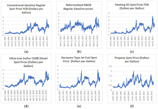
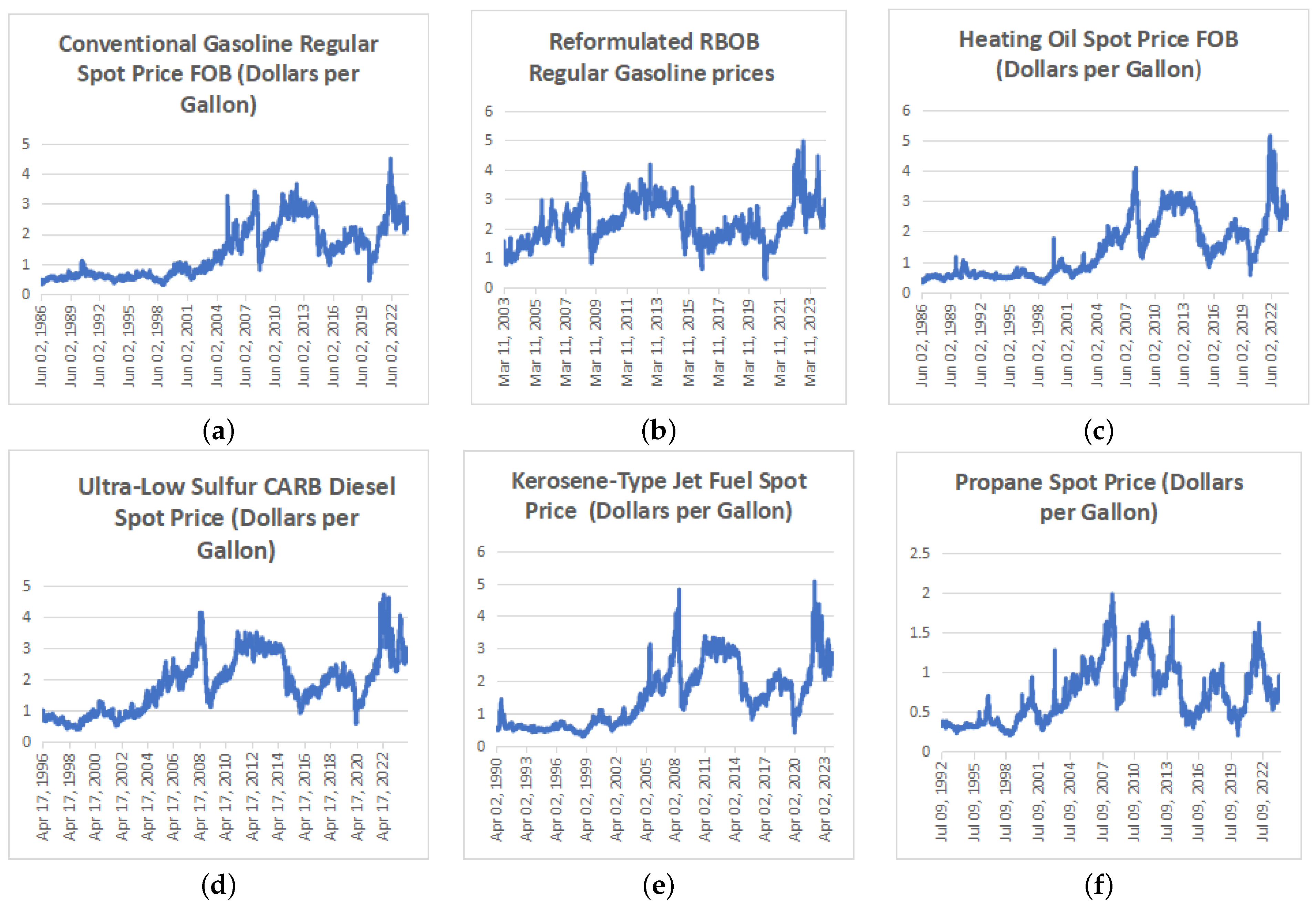
To rigorously evaluate the proposed RAD framework, six daily spot price datasets for petroleum products were analyzed, covering extended periods and heterogeneous market conditions. These include New York Conventional Gasoline (2 June 1986–18 March 2024), Los Angeles Reformulated RBOB Gasoline (11 March 2003–18 March 2024), New York Heating Oil (2 June 1986–18 March 2024), and Los Angeles Ultra-Low Sulfur No. 2 Diesel (17 April 1996–18 March 2024), U.S. Gulf Coast Kerosene-Type Jet Fuel (2 April 1990–18 March 2024), and Mont Belvieu Propane (9 July 1992–18 March 2024). Figure 2 depicts the historical price dynamics of the six petroleum products: Conventional Gasoline, Reformulated RBOB Gasoline, Heating Oil, Ultra-Low Sulfur CARB Diesel, Kerosene-Type Jet Fuel, and Propane. A long-term upward trend is evident across all series, reflecting sustained increases in global oil prices. Superimposed on this gradual growth are sharp fluctuations associated with major geopolitical shocks, economic crises, and disruptions in supply-demand balances. Two pronounced surges are clearly visible: the 2008 peak during the global financial crisis, followed by a rapid collapse, and the 2021–2022 spike driven by post-pandemic recovery and supply chain constraints. Distinct differences in volatility structures can also be observed. Propane and Kerosene demonstrate higher short-term variability, with multiple rapid oscillations, whereas Heating Oil and Diesel exhibit comparatively smoother price trajectories with well-defined peaks. Despite these variations, the co-movement across fuels remains strong, highlighting their interdependence and exposure to common macroeconomic drivers. These patterns motivate the application of decomposition techniques such as RAD, which can disentangle local fluctuations from long-term trends and capture both symmetric and asymmetric dynamics inherent in the data.

Figure 2. Plots of all oil prices used in the study. Each subfigure represents the historical price trend of a specific oil product over the study period.

4.2. Descriptive Statistics

Table 1 presents summary statistics for these series, providing insights into their volatility and asymmetry patterns. Among the commodities, Heating Oil exhibited the highest maximum price (USD 5.152), closely followed by Jet Fuel (USD 5.066) and Reformulated RBOB Gasoline (USD 4.968), whereas Propane demonstrated the lowest overall range (USD 0.203–1.980), reflecting its lower market valuation and relative stability. The mean price levels further highlight market heterogeneity, with Reformulated RBOB Gasoline being the most expensive (mean = USD 2.184), followed by Ultra-Low Sulfur Diesel (USD 1.839) and Jet Fuel (USD 1.519). Dispersion patterns also varied significantly: Conventional Gasoline and Heating Oil presented wide distributions, indicative of historical shocks and market cycles, while Propane displayed a narrow interquartile range (USD 0.396–0.973) and low median (USD 0.645), emphasizing structural stability. These statistics underscore the diverse asymmetries and stochastic features that challenge traditional decomposition and forecasting methods, and illustrate the need for robust approaches such as RAD.

Table 1. Summary statistics of oil and fuel spot prices (in USD per gallon).

Product	Min	1st Quartile	Median	Mean	3rd Quartile	Max
Conventional Gasoline (NY)	0.290	0.595	1.177	1.389	2.059	4.509
Reformulated RBOB Gasoline (LA)	0.293	1.661	2.148	2.184	2.697	4.968
Heating Oil (NY)	0.284	0.560	1.145	1.413	2.015	5.152
ULS CARB Diesel (LA)	0.375	0.955	1.837	1.839	2.480	4.739
Kerosene-Type Jet Fuel (USGC)	0.282	0.618	1.384	1.519	2.135	5.066
Propane (Mont Belvieu)	0.203	0.396	0.645	0.724	0.973	1.980

An Intrinsic Mode Function (IMF) is considered noise if it satisfies three diagnostic conditions: (i) it conveys no significant information content, (ii) it has a mean approximately equal to zero, and (iii) it exhibits randomness. To formally assess these properties, three complementary statistical measures were employed: permutation entropy (to quantify hidden information), the Ljung-Box (LB) test (to evaluate randomness), and the arithmetic mean (to verify centering around zero). The results of these diagnostics, reported in Table 2, provide an empirical basis for distinguishing meaningful IMFs from noise across all datasets.

Table 2. Statistical measures for noise property checking of IMF components.

IMF (Noise) Component	Permutation Entropy	Mean	Ljung-Box Test (p-Value)
Conventional Gasoline Regular Spot Price	0.9983	−0.000	0.2291
Reformulated RBOB Regular Gasoline Prices	0.9975	−0.000	0.0512
Heating Oil Spot Price FOB	0.9988	−0.000	0.2871
Ultra-Low Sulfur CARB Diesel Spot Price	0.9976	−0.000	0.4823
Kerosene-Type Jet Fuel Spot Price	0.9987	−0.000	0.5462
Propane Spot Price	0.9955	−0.000	0.2463

As reported in Table 2, the diagnostic measures consistently confirm the noisy nature of the extracted IMFs. First, the permutation entropy values remain uniformly high (0.9955–0.9988), reflecting a near-complete absence of structured or deterministic information. Such values imply that the IMFs behave like random sequences, exhibiting no discernible patterns or symmetry-breaking dynamics that could contribute to meaningful signal reconstruction. Second, the mean values are negligibly close to zero across all series, confirming that the oscillations are centered and unbiased, which is a necessary property of pure noise components. Third, the Ljung-Box (LB) test results further reinforce these observations: all p-values (0.0512–0.5462) exceed the conventional 0.05 threshold, indicating no statistical evidence against the null hypothesis of randomness. Taken together, these diagnostics establish that the examined IMFs predominantly represent stochastic noise rather than informative structural components. This validation step is critical for the RAD framework, as it ensures that only significant and interpretable modes are retained for further analysis, while systematically filtering out spurious oscillations. By enforcing this criterion, the decomposition process not only enhances robustness but also preserves the original signal’s underlying temporal symmetry, thereby providing a more reliable foundation for forecasting and interpretation.

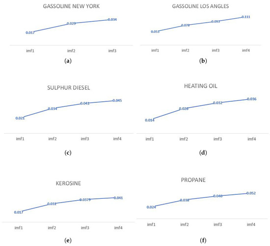
Figure 3 illustrates the correlation coefficients between the original oil price series and their corresponding Intrinsic Mode Functions (IMFs), ranging from IMF1 to IMF4. Several important patterns can be observed across different petroleum products. First, all series display a consistent upward trend in correlations as the decomposition progresses from high-frequency (IMF1) to lower-frequency components (IMF4). This indicates that higher-order IMFs, which capture smoother, longer-term oscillations, preserve stronger associations with the underlying price dynamics than the short-term, noise-dominated components. For example, the Los Angeles Gasoline series shows a pronounced increase in correlation, from 0.025 for IMF1 to 0.111 for IMF4, highlighting the strong influence of trend-like components on its price evolution. A similar, though less intense, trajectory is evident in New York Gasoline, where correlations rise from 0.017 to 0.034. Other fuels, such as Heating Oil and Sulfur Diesel, exhibit comparable behaviors, with correlations peaking at 0.036 and 0.045, respectively. Kerosene shows a gradual rise, reaching 0.041 at IMF4, while Propane exhibits the most linear, steadily increasing pattern, beginning at 0.022 and peaking at 0.052, suggesting a clearer temporal dependency on its decomposed components.

Figure 3. Line plot representing the correlation coefficient between different oil prices and each IMF.

For this study, the EEMD and CEEMDAN methods were implemented using the libeemd library, introduced by Petteri J. J. Luukko, Jouni Helske, and Eero Räsänen [65]. As the authors suggested and in accordance with the best practices in the decomposition methods literature, the standard settings for the parameters provided by the library were used: Ensemble size: 250 realizations Noise strength: 0.2* standard deviation of the original signal These settings are widely used in the existing literature because they effectively balance reducing mode-mixing with improving efficiency. It is also important to emphasize that these parameters are not designed to minimize forecasting error metrics; rather, they are algorithmic parameters that control the robustness and statistical consistency of the methods’ results.

From a methodological perspective, these findings provide two critical insights. First, the increasing correlation trend across IMFs implies that lower-frequency components (IMF3 and IMF4) capture structural variations that are more closely aligned with the deterministic dynamics of oil price movements. This observation is consistent with the theoretical expectation that long-term modes contain more meaningful economic information, whereas high-frequency IMFs are dominated by stochastic fluctuations. Second, the monotonic rise in correlation suggests incomplete separation in the traditional EMD-based framework, as later IMFs retain fragments of the original deterministic signal rather than achieving full orthogonality. In this context, the RAD algorithm introduces an adaptive stopping criterion: once the correlation begins to increase after decreasing, the decomposition halts. This ensures that residual deterministic structures are not mistakenly treated as noise, thereby preserving the temporal symmetry and interpretability of the resulting components. However, the correlation analysis underscores the importance of robust decomposition strategies in distinguishing between noise and signal in volatile energy markets. By adaptively controlling the sifting process, RAD avoids over-decomposition, enhances mode separation, and provides a more reliable foundation for downstream forecasting tasks.

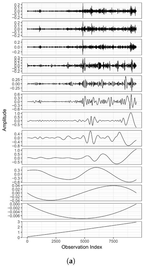
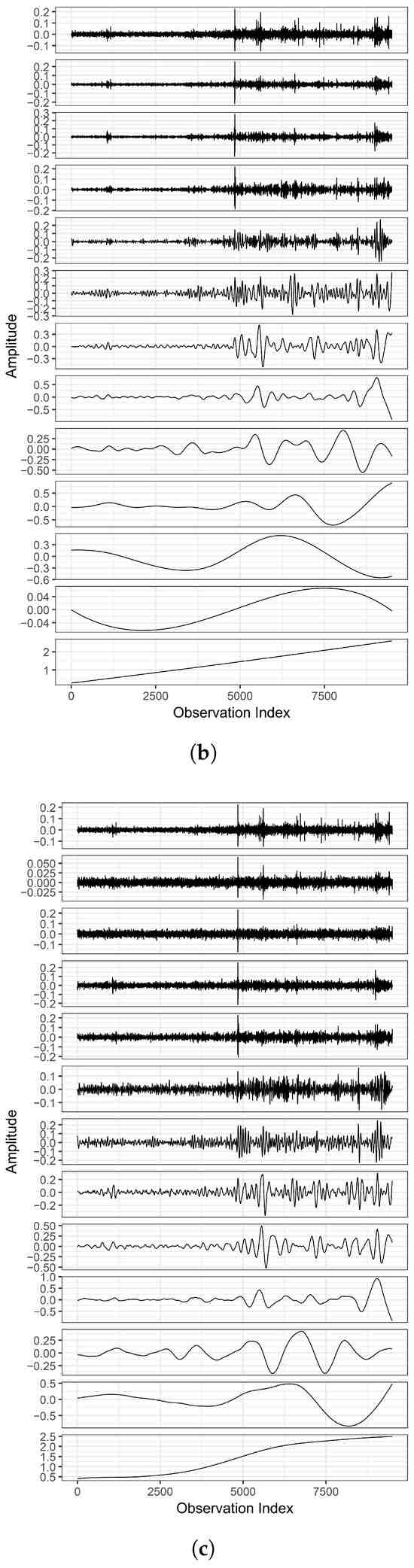
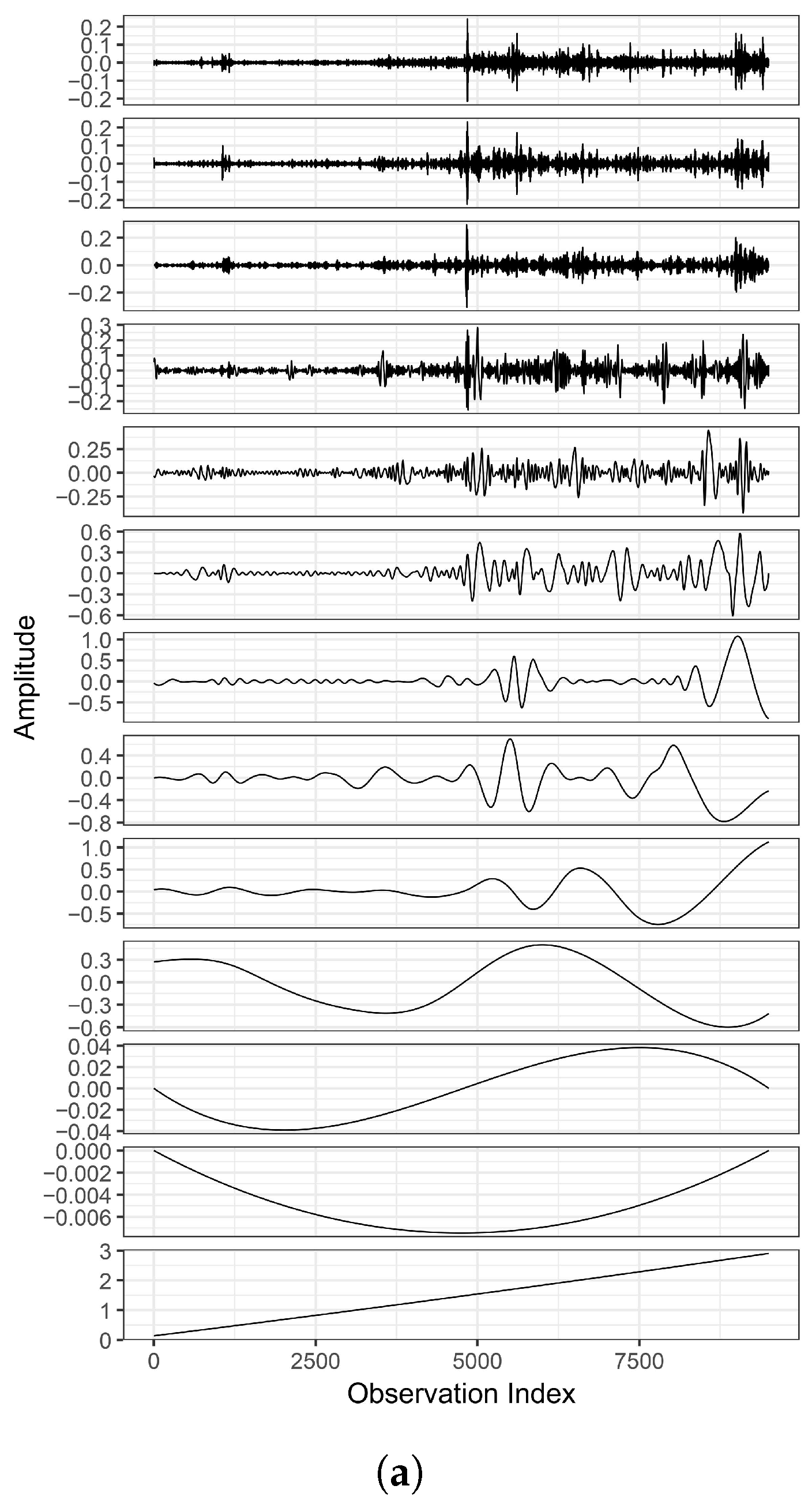
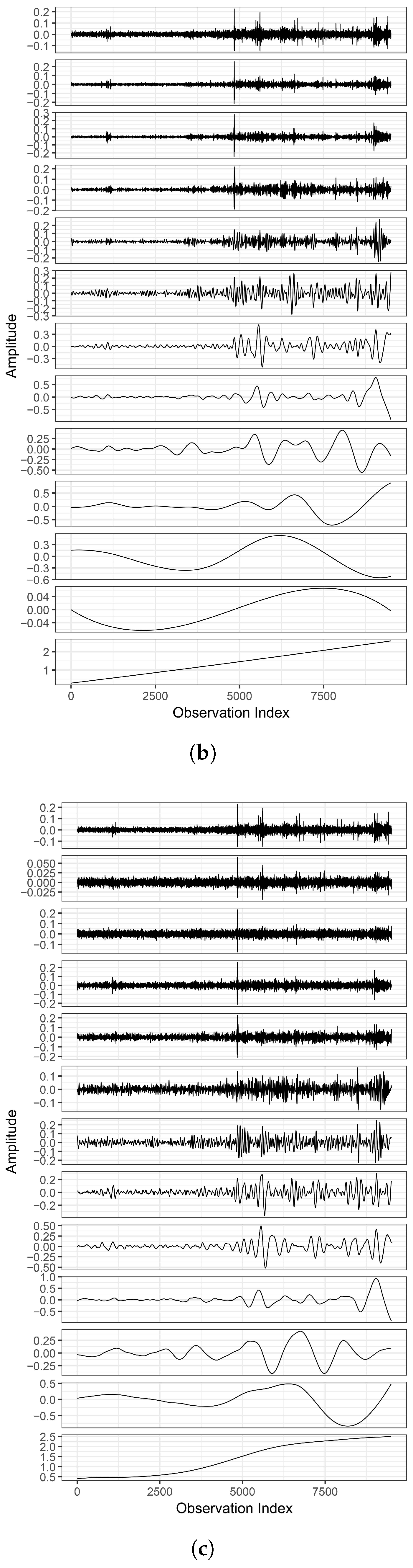
For this study, the EEMD and CEEMDAN methods were implemented using the libeemd library, introduced by Petteri J. J. Luukko et al. [65]. As the authors suggested and in accordance with the best practices in the decomposition methods literature, the standard settings for the parameters provided by the library were used: Ensemble size: 250 realizations; Noise strength: 0.2 times the standard deviation of the original signal. These settings are widely used in existing literature because they effectively balance reducing mode-mixing with improving efficiency. It is also important to emphasize that these parameters are not designed to minimize forecasting error metrics; rather, they are algorithmic parameters that control the robustness and statistical consistency of the methods’ results. The number of IMFs was not predetermined or truncated by hand. In EMD and EMD-like algorithms, it is natural that the number of IMFs grows adaptively from the process itself and depends only on the intrinsic oscillatory characteristics of the given signal. It would therefore be unnatural and risky to artificially constrain or fix it by hand. We therefore let it grow naturally according to the process’s natural stopping criteria [78,79,80,81], as mentioned in previous studies. To exemplify this structural characteristic of the decomposition, Figure 4 shows the complete set of decomposed IMFs, thereby demonstrating that the obtained components represent progressively lower-frequency oscillatory modes, indicating that the decomposition was indeed controlled by the internal structure of the signal, rather than by externally set predictive goals. Thus, the ensemble size and noise level were treated as structural parameters to ensure the stability of the decomposition method, whereas the number of IMFs was determined entirely data-driven. These parameters were not optimized to achieve a minimum in forecasting performance metrics such as MAE and MAPE.

Figure 4. Plots (a–c) illustrate the decomposition of Intrinsic Mode Functions (IMFs) achieved through EMD, EEMD, and CEEMDAN, respectively.

4.3. Model Development and Experimental Setup

For model development, each series was split into training and testing sets, with 80% of observations allocated for training and 20% reserved for testing. This ensures a robust assessment of generalization performance. Forecasting models included ARIMA, ARFIMA, LSTM, and XGBoost. ARIMA and ARFIMA serve as classical and long-memory linear benchmarks, respectively. ARIMA models were implemented via the auto.arima function in R, selecting optimal lag orders based on information criteria. ARFIMA models, implemented using the arfima package, employ fractional differencing to capture long-range dependencies in price series. Nonlinear machine learning models included LSTM networks, constructed with two hidden layers of 50 units each, a dense output layer, and dropout regularization (rate 0.2) to mitigate overfitting. Input data were Min–Max normalized and structured via sliding windows to predict one-step-ahead values. XGBoost models were trained as gradient-boosted ensembles of regularized decision trees, with hyperparameters tuned for learning rate, tree depth, subsampling ratio, and regularization terms to optimize predictive performance while controlling complexity.

Regarding hyperparameter selection, during the analysis phase, this work systematically explored a range of candidate values for key parameters (such as learning rate, number of layers, number of filters/neurons, and kernel size) by incrementally increasing and decreasing them. The objective was to identify configurations that minimized forecasting error on the validation data. Parameters that led to higher error rates or unstable predictions were discarded. The final parameters reported in the manuscript correspond to these tuned values, which consistently produced lower prediction errors and more stable model performance. Therefore, the reported hyperparameters are not arbitrary but represent empirically tuned settings selected after extensive experimentation. Also, Seasonal modeling approaches, such as SARIMA, were carefully considered in our analysis. As shown in Figure 2, the time-series plots do not exhibit any clear or recurring seasonal pattern. This visual assessment suggests that seasonality is weak or absent in the data. Nevertheless, to ensure that no seasonal structure was overlooked, we employed the auto.arima() function from the forecast package in R. This procedure automatically tests for both non-seasonal and seasonal components and selects a SARIMA model when seasonality is statistically supported. In our case, auto.arima() consistently selected a non-seasonal ARIMA specification, confirming the absence of significant seasonal effects in the series. Therefore, seasonal models were not included, as they did not improve model fit or forecasting performance.

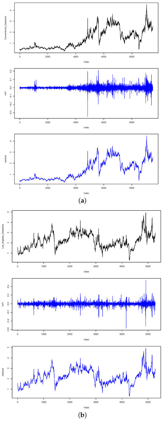
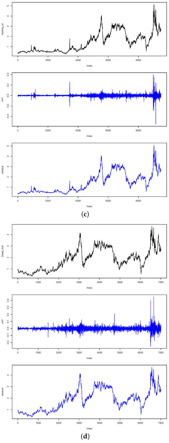
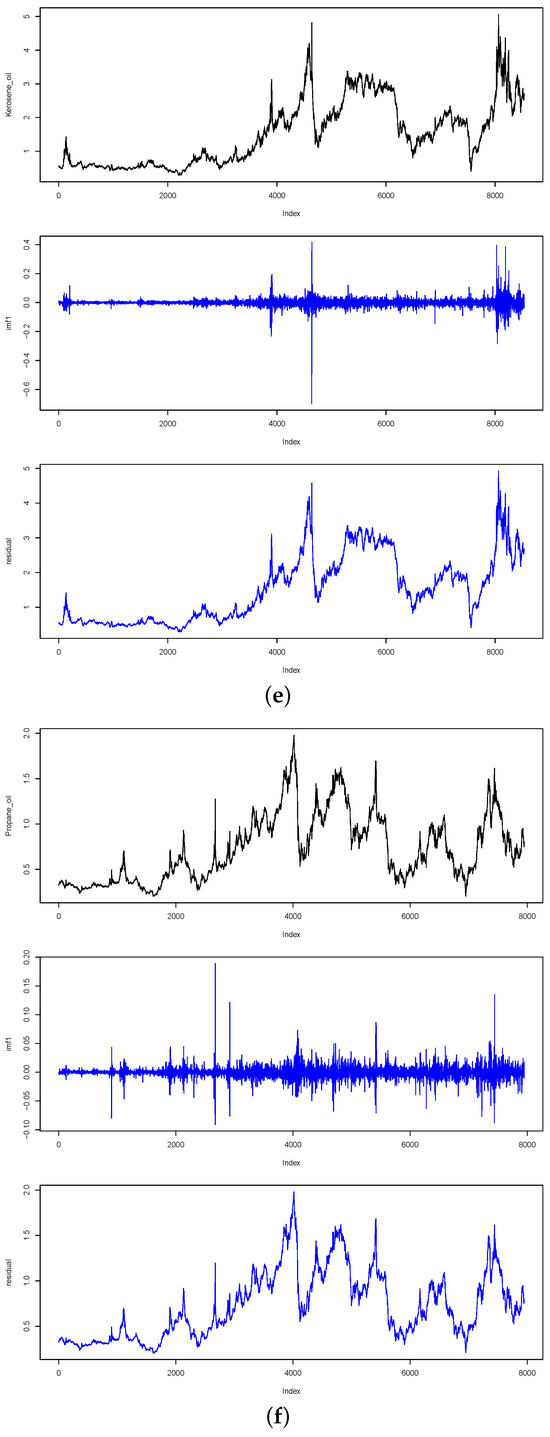
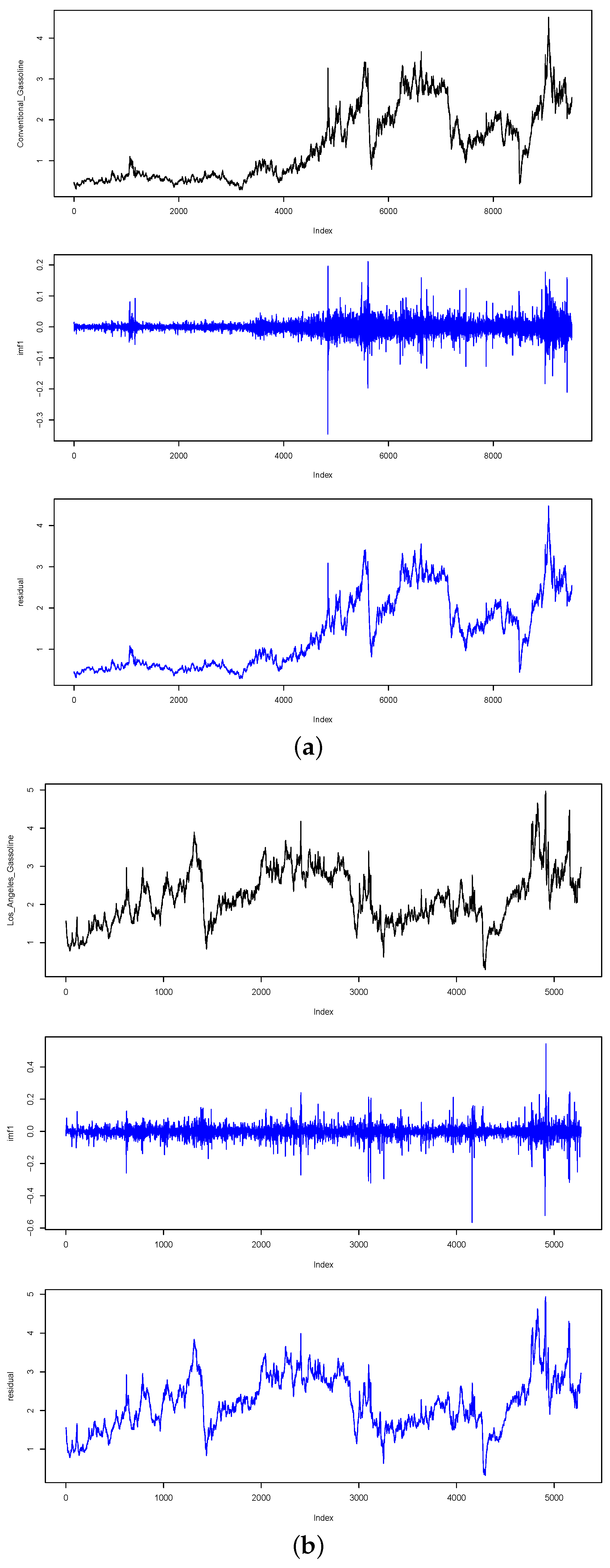
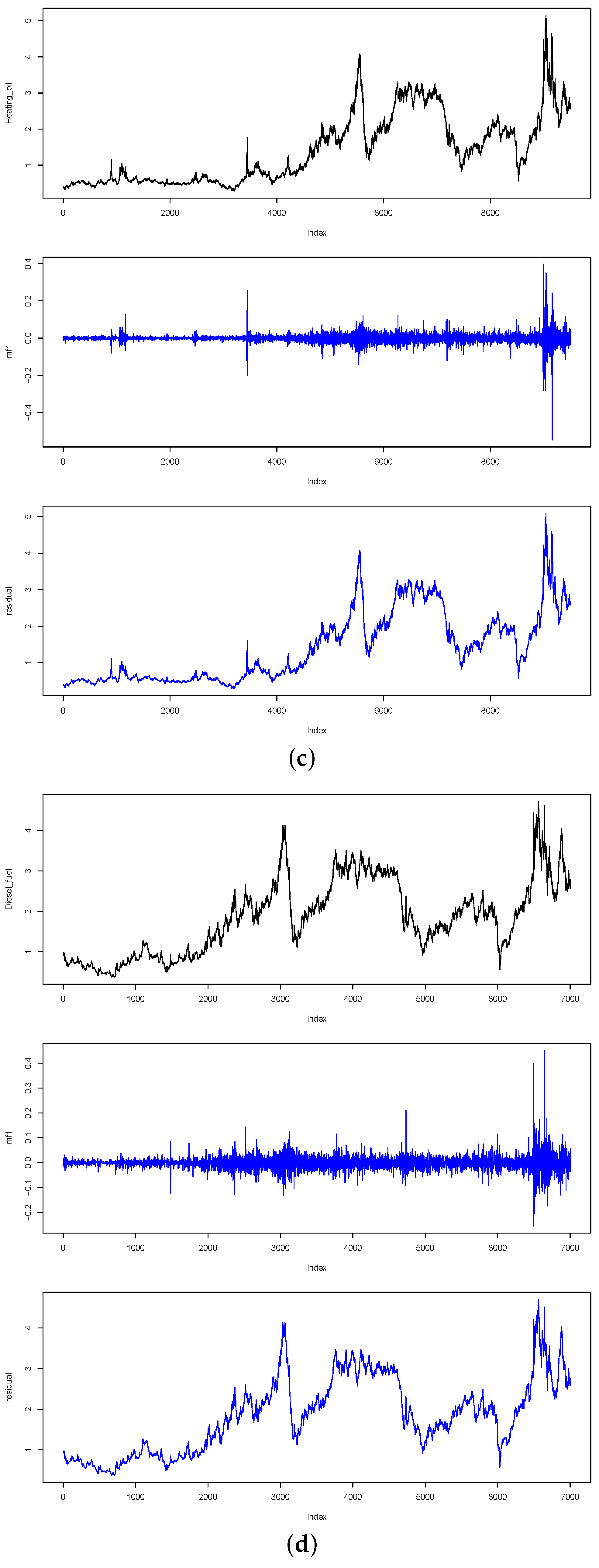
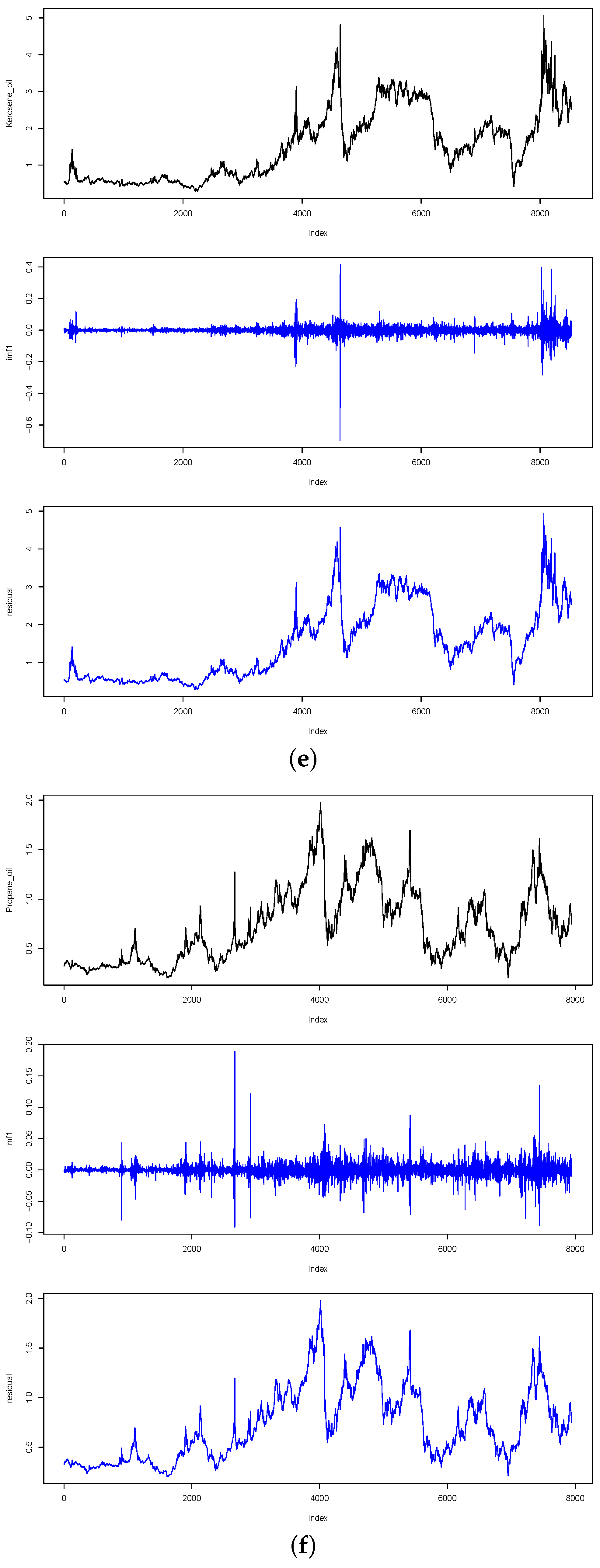
On the other hand, Figure 5a–f presents the decomposition results obtained using the proposed RAD algorithm across six representative energy commodities: Figure 5a Gasoline (New York), Figure 5b Gasoline (Los Angeles), Figure 5c Heating Oil, Figure 5d Sulphur Diesel Oil, Figure 5e Kerosene Oil, and Figure 5f Propane Oil. Each subfigure is structured into three vertically arranged panels: the original series (top), the first Intrinsic Mode Function (IMF) capturing high-frequency oscillations (middle), and the residual component reflecting long-term dynamics (bottom). This visual arrangement highlights the symmetry in the decomposition of short-term volatility and long-term structural behavior. In all cases, the high-frequency IMFs (middle panels) exhibit rapid oscillations centered around zero, consistent with stochastic fluctuations and cyclical noise. For instance, Gasoline (New York) and Gasoline (Los Angeles) both display sharp localized spikes in the IMF, indicating demand-supply shocks and seasonal effects. Conversely, the residuals (bottom panels) reveal smooth, persistent trends, which capture the deterministic structure of the series. Notably, Heating Oil Figure 5c and Sulphur Diesel Oil Figure 5d exhibit pronounced upward drifts in their residuals, reflecting structural price adjustments driven by macroeconomic conditions and regulatory interventions. Propane Oil Figure 5f shows a clear upward structural trend toward the end of the observation period, indicating latent pricing pressures not visible in the noisy IMF component. These findings underscore RAD’s ability to separate noisy short-term variations from meaningful long-term structures while preserving the intrinsic symmetry of the original signal.

Figure 5. Plots (a–f) illustrate the Intrinsic Mode Functions (IMFs) and residual components obtained using the Robust Adaptive Decomposition technique for six oil price series: (a) Gasoline (New York), (b) Gasoline (Los Angeles), (c) Heating Oil, (d) Sulphur Diesel Oil, (e) Kerosene Oil, and (f) Propane Oil.

4.4. Forecasting Results

In this work, the RAD framework was first applied to each commodity series to decompose deterministic and stochastic components. Forecasts were generated on reconstructed series using ARIMA, ARFIMA, LSTM, and XGBoost, allowing evaluation of the impact of robust decomposition on predictive accuracy. For comparison, benchmark decomposition methods (EMD, EEMD, and CEEMDAN) were also integrated with the same forecasting models. Forecasting accuracy was quantified using Mean Absolute Error (MAE), Root Mean Square Error (RMSE), Mean Absolute Percentage Error (MAPE), and Directional Accuracy (DA), ensuring a comprehensive assessment across absolute, relative, and directional criteria.

The forecasting accuracy results reported in Table 3 incorporate four key forecasting evaluation metrics—MAE, RMSE, MAPE, and Directional Accuracy (DA)—across five predictive model classes (ARIMA, LSTM, XGBOOST, ARFIMA, and their hybrid decomposed variants). The inclusion of DA enables a more comprehensive analysis of trend prediction capabilities beyond absolute and relative error magnitudes. In both the New York and Los Angeles Gasoline markets, RAD-ARIMA remains the dominant performer, yielding drastic reductions in MAE and MAPE while achieving DA values above 90%, indicating exceptional trend-capturing capability. Although EEMD and CEEMDAN occasionally achieve competitive DA, they fail to match RAD’s consistently low error magnitudes, underscoring RAD’s balanced performance between accuracy and signal directionality. In LSTM and XGBOOST settings, RAD-based models generally outperform their empirical-mode counterparts, though the magnitude of improvement varies by commodity, reflecting model–signal alignment effects.

Table 3. Forecasting performance metrics (MAE, RMSE, MAPE, DA) of RAD, EMD, EEMD, and CEEMDAN-based hybrid models across various oil commodity datasets.

Model	MAE	RMSE	MAPE	DA
Gasoline Oil (New York)
ARIMA	0.0376	0.0556	1.9299	50.34%
RAD-ARIMA	0.0048	0.0080	0.2375	92.26%
EMD-ARIMA	0.0210	0.0307	1.0976	66.43%
EEMD-ARIMA	0.2343	0.2891	14.7545	82.78%
CEEMDAN-ARIMA	0.3114	0.4206	15.8933	78.41%
LSTM	0.0397	0.0586	2.0459	53.87%
RAD-LSTM	0.1265	0.1593	6.7670	69.12%
EMD-LSTM	0.0445	0.0636	2.2314	73.21%
EEMD-LSTM	0.0560	0.0812	2.8234	78.43%
CEEMDAN-LSTM	0.0465	0.0681	2.3676	79.67%
XGBOOST	0.0542	0.1156	2.44	44.84%
RAD-XGBOOST	0.0383	0.1105	1.58	68.23%
EMD-XGBOOST	0.3033	0.4486	13.09	72.13%
EEMD-XGBOOST	0.2285	0.2980	7.40	82.81%
CEEMDAN-XGBOOST	0.2184	0.2691	10.67	72.97%
ARFIMA	3.9541	3.9550	218.05	50.92%
RAD-ARFIMA	2.6608	2.6618	146.37	70.35%
EMD-ARFIMA	2.1685	2.1700	83.44	66.82%
EEMD-ARFIMA	2.9945	2.9955	127.83	72.30%
CEEMDAN-ARFIMA	1.6761	1.6780	69.76	71.56%
Gasoline Oil (Los Angeles)
ARIMA	0.0647	0.1092	2.8601	49.87%
RAD-ARIMA	0.0102	0.0208	0.5852	91.27%
EMD-ARIMA	0.0355	0.0560	1.5063	56.86%
EEMD-ARIMA	0.1949	0.2351	9.5204	85.12%
CEEMDAN-ARIMA	0.2040	0.2301	10.3643	79.43%
LSTM	0.0745	0.1234	2.9765	61.78%
RAD-LSTM	0.0898	0.1487	4.0503	67.89%
EMD-LSTM	0.0932	0.2389	5.9763	71.45%
EEMD-LSTM	0.0898	0.1487	5.9655	83.71%
CEEMDAN-LSTM	0.0878	0.1384	4.0839	70.67%
XGBOOST	0.0810	0.3410	2.3650	45.81%
RAD-XGBOOST	0.0728	0.1685	4.58	70.59%
EMD-XGBOOST	0.3796	0.4616	15.63	74.95%
EEMD-XGBOOST	0.1609	0.2366	7.36	79.98%
CEEMDAN-XGBOOST	0.2353	0.2998	10.28	78.37%
ARFIMA	2.5476	3.7840	5.78	52.97%
RAD-ARFIMA	0.4308	0.4498	23.71	69.07%
EMD-ARFIMA	2.3520	2.3569	118.48	66.13%
EEMD-ARFIMA	2.9605	2.9642	149.56	74.48%
CEEMDAN-ARFIMA	3.8243	3.8272	193.73	72.49%
Heating Oil
ARIMA	3.2460	5.0807	2.3726	51.51%
RAD-ARIMA	0.0050	0.0149	0.2735	93.56%
EMD-ARIMA	11.3183	12.5772	8.8241	67.46%
EEMD-ARIMA	17.5562	22.2615	13.0612	70.45%
CEEMDAN-ARIMA	29.0035	33.4143	21.4131	68.67%
LSTM	3.2748	5.0417	2.3927	74.76%
RAD-LSTM	5.3996	8.0813	3.8850	63.89%
EMD-LSTM	4.3534	6.2911	3.1591	73.45%
EEMD-LSTM	5.2678	7.8989	3.7326	71.81%
CEEMDAN-LSTM	3.8426	5.8154	2.7563	73.76%
XGBOOST	0.0603	0.1354	2.39	46.73%
RAD-XGBOOST	0.0412	0.1191	1.49	67.39%
EMD-XGBOOST	0.2128	0.3190	9.09	73.18%
EEMD-XGBOOST	0.2895	0.3974	12.24	77.19%
CEEMDAN-XGBOOST	0.2895	0.3974	12.24	77.19%
ARFIMA	8.0140	8.0155	269.68	52.52%
RAD-ARFIMA	3.2001	3.2014	171.39	71.41%
EMD-ARFIMA	4.4142	4.4154	236.71	65.46%
EEMD-ARFIMA	2.9742	2.9758	159.24	72.78%
CEEMDAN-ARFIMA	2.5204	2.5224	134.82	69.67%
Sulphur Diesel Oil
ARIMA	2.0960	3.4079	2.0763	50.11%
RAD-ARIMA	0.0073	0.01579	0.2859	92.34%
EMD-ARIMA	1.3036	2.0418	1.2942	70.64%
EEMD-ARIMA	1.1133	1.6700	1.1161	85.98%
CEEMDAN-ARIMA	0.9597	1.3855	0.9799	75.10%
LSTM	2.7684	3.6734	2.0932	53.89%
RAD-LSTM	1.1432	1.8338	1.1244	69.81%
EMD-LSTM	1.8421	2.3476	1.8993	71.89%
EEMD-LSTM	1.7854	2.6012	1.8228	86.78%
CEEMDAN-LSTM	1.7961	2.6069	1.8537	84.89%
XGBOOST	0.0633	0.1126	2.45	49.54%
RAD-XGBOOST	0.0401	0.0879	1.45	70.55%
EMD-XGBOOST	0.3683	0.5341	13.28	72.84%
EEMD-XGBOOST	0.1130	0.1992	4.05	79.34%
CEEMDAN-XGBOOST	0.1064	0.1760	4.20	74.41%
ARFIMA	0.9122	0.9196	43.13	52.07%
RAD-ARFIMA	2.1309	2.1333	102.03	70.79%
EMD-ARFIMA	2.6324	2.6349	126.19	66.86%
EEMD-ARFIMA	2.2711	2.2737	108.77	72.43%
CEEMDAN-ARFIMA	2.8137	2.8158	134.97	73.93%
Kerosine Oil
ARIMA	1.9312	3.2843	2.1132	51.64%
RAD-ARIMA	0.3624	0.7191	0.4044	87.87%
EMD-ARIMA	1.1455	1.8511	1.2506	64.67%
EEMD-ARIMA	0.8292	1.2189	0.9579	81.23%
CEEMDAN-ARIMA	0.9166	1.3547	1.0483	78.92%
LSTM	2.6809	4.2519	2.4084	63.98%
RAD-LSTM	1.5856	2.5903	1.4224	67.48%
EMD-LSTM	2.6831	3.7391	2.5440	66.12%
EEMD-LSTM	1.8727	2.7516	1.7434	80.78%
CEEMDAN-LSTM	1.8035	2.6236	1.7328	79.99%
XGBOOST	0.0543	0.0954	2.43	48.04%
RAD-XGBOOST	0.0328	0.0667	1.40	67.68%
EMD-XGBOOST	0.2943	0.4325	12.18	74.84%
EEMD-XGBOOST	0.1189	0.1663	5.37	79.12%
CEEMDAN-XGBOOST	0.1526	0.2346	6.15	72.43%
ARFIMA	10.7271	10.7276	586.68	50.00%
RAD-ARFIMA	11.5145	11.5149	629.85	69.70%
EMD-ARFIMA	1.6617	1.6649	90.01	67.35%
EEMD-ARFIMA	1.9042	1.9069	103.28	72.98%
CEEMDAN-ARFIMA	2.1097	2.1122	114.56	72.63%
Propane Oil
ARIMA	0.6312	0.9959	2.0166	61.80%
RAD-ARIMA	0.1132	0.1985	0.3467	90.12%
EMD-ARIMA	5.2056	5.8681	16.9727	63.23%
EEMD-ARIMA	8.9911	9.9825	31.2124	80.11%
CEEMDAN-ARIMA	4.4012	4.9769	15.0829	77.66%
LSTM	0.8843	1.2379	2.7748	67.88%
RAD-LSTM	0.6468	0.8853	1.9673	69.90%
EMD-LSTM	0.6468	0.8853	1.9673	68.13%
EEMD-LSTM	0.7289	0.9313	1.8547	88.79%
CEEMDAN-LSTM	0.5572	0.7296	1.8547	86.76%
XGBOOST	0.0169	0.0255	2.24	47.61%
RAD-XGBOOST	0.0091	0.0137	1.21	65.81%
EMD-XGBOOST	0.1603	0.1996	20.39	67.32%
EEMD-XGBOOST	0.0281	0.0423	3.39	71.79%
CEEMDAN-XGBOOST	0.0139	0.0232	1.65	67.57%
ARFIMA	0.9233	0.9240	131.46	55.57%
RAD-ARFIMA	0.7941	0.7948	112.96	71.05%
EMD-ARFIMA	0.7826	0.7834	111.37	67.15%
EEMD-ARFIMA	0.9242	0.9249	131.64	72.31%
CEEMDAN-ARFIMA	1.1860	1.1865	169.15	70.04%

In more volatile commodities such as Heating Oil and Sulphur Diesel Oil, the superiority of RAD becomes even more pronounced. RAD-ARIMA achieves orders-of-magnitude lower MAE and MAPE compared to EMD, EEMD, and CEEMDAN, with DA values exceeding 92% in multiple cases. This highlights the fundamental advantage of RAD’s robust adaptive separation mechanism, which effectively mitigates mode mixing and over-decomposition, preventing noise contamination of predictive components. Even when paired with deep learning (LSTM) or tree-based methods (XGBOOST), RAD maintains consistently competitive performance, demonstrating its flexibility across forecasting architectures. On the other hand, the results for Kerosene Oil reveal a similar pattern: RAD-ARIMA vastly outperforms all benchmark decompositions, confirming its suitability for medium-volatility datasets. RAD-LSTM also provides consistent improvements in MAPE and DA, though the relative gains are more moderate, reflecting the interplay between decomposition structure and network learning dynamics. While the Propane Oil provides the most dramatic evidence of RAD’s robustness. Across all forecasting families—ARIMA, LSTM, XGBOOST, and ARFIMA—RAD-based models dominate in both MAE/MAPE reduction and DA enhancement. The exceptionally low errors of RAD-ARIMA (MAE = 0.1132, MAPE = 0.3467, DA = 90.12%) and RAD-XGBOOST (MAE = 0.0091) demonstrate that RAD is uniquely capable of extracting structurally meaningful modes in noisy, small-range energy price series. Thus, taken together, the updated results provide more substantial and more comprehensive support for the argument that RAD offers a superior decomposition paradigm for nonlinear, nonstationary, and volatile commodity markets. Its scale-based adaptive weighing, noise-robust stopping rule, and symmetric mode extraction lead not only to reduced error magnitudes but also substantially improved directional accuracy—an essential property for risk-sensitive financial forecasting. Through consistent dominance across multiple commodities and forecasting models, RAD positions itself as a next-generation robust time-frequency decomposition method for real-world energy analytics.

Thus, the empirical evidence decisively confirms that the proposed RAD method substantially enhances forecasting performance across diverse oil commodity datasets and modeling frameworks. Among the evaluated configurations, the RAD-ARIMA hybrid consistently achieves the best performance, yielding the lowest forecast errors and demonstrating superior robustness to structural breaks, market shocks, and regime shifts. This advantage stems from RAD’s ability to effectively disentangle high-frequency noise-like components from meaningful low-frequency structures, thereby preserving both short-term fluctuations and long-term dynamics in a balanced manner. The results further highlight RAD’s adaptability in handling the inherent nonlinearity and non-stationarity of energy price series, which pose significant challenges for conventional decomposition methods. By systematically outperforming EMD-, EEMD-, and CEEMDAN-based models in both statistical (ARIMA) and deep learning (LSTM) settings, RAD validates not only its theoretical soundness but also its empirical utility in real-world forecasting tasks. Consequently, these findings establish RAD as a powerful and generalizable signal decomposition technique, with broad applicability in applied econometrics, energy economics, and financial forecasting. In this regard, RAD advances the methodological frontier of time series analysis within the scope of symmetry-driven decomposition and predictive modeling, offering a substantial improvement over classical empirical mode decompositions.

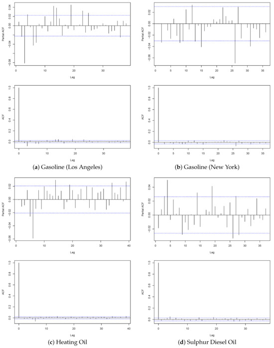
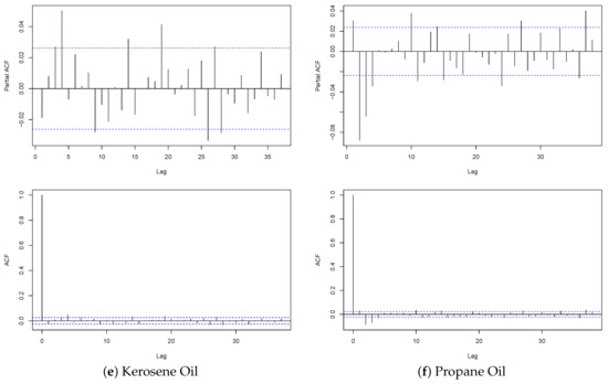
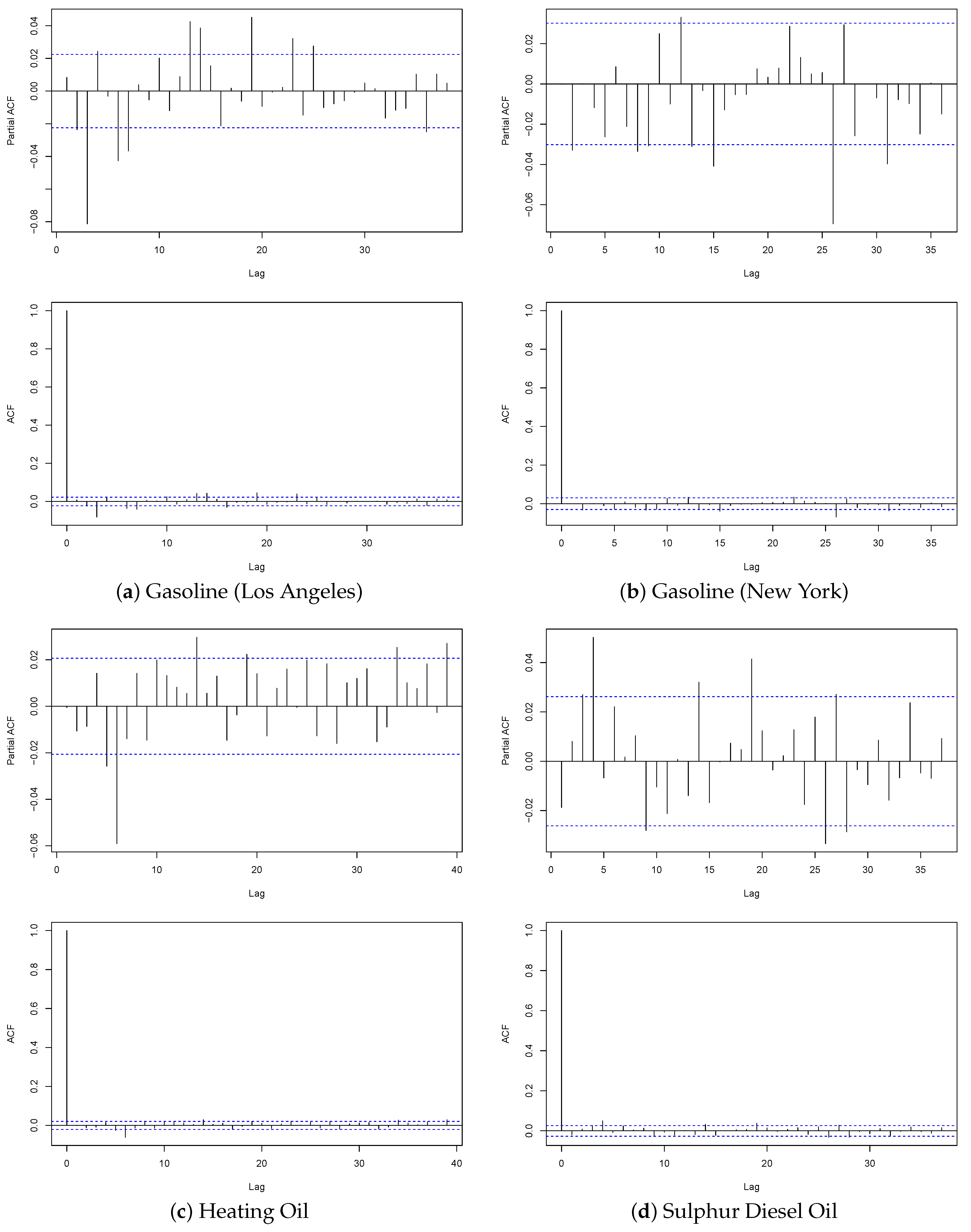
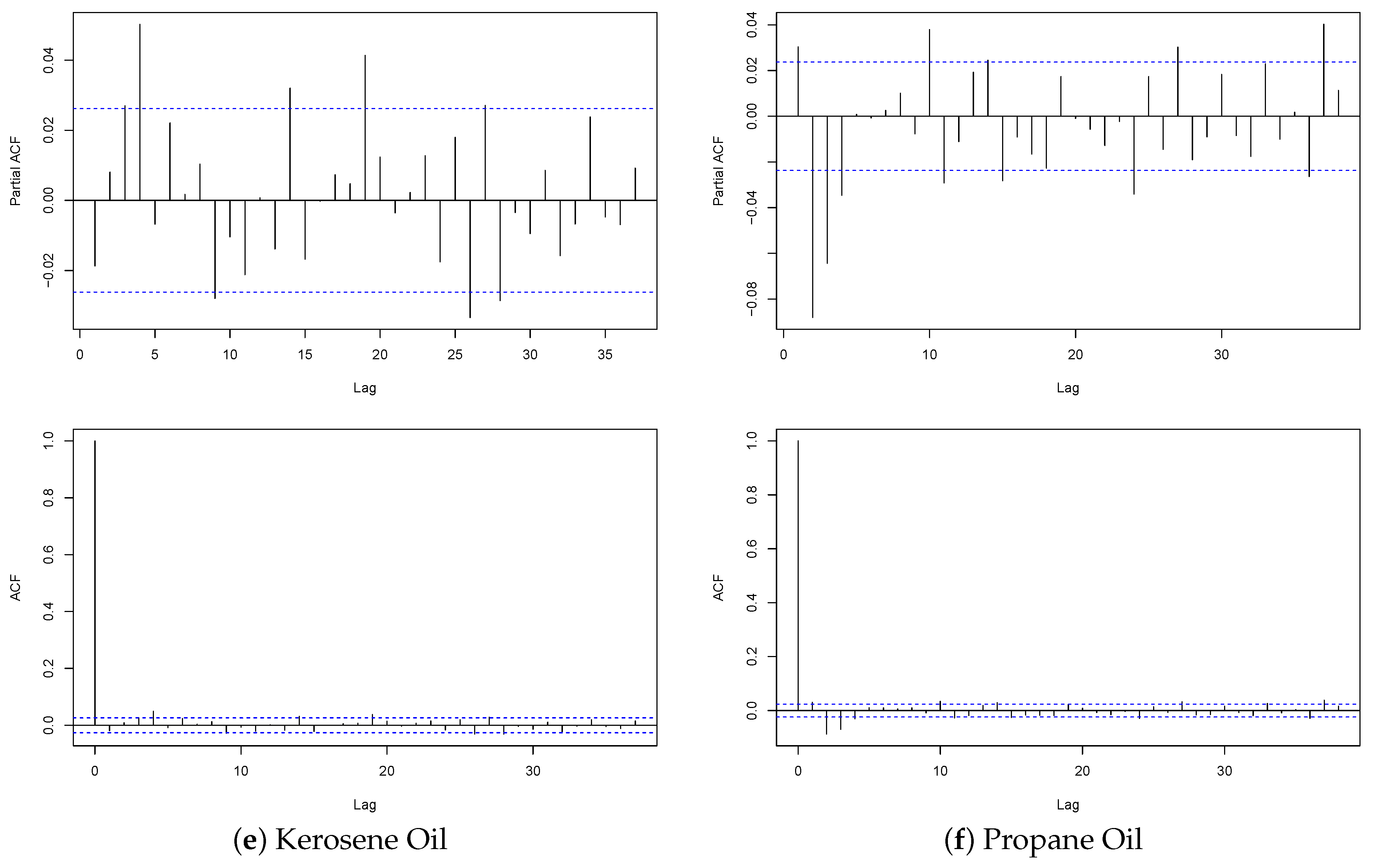
Figure 6 displays the Partial Autocorrelation Function (PACF) and Autocorrelation Function (ACF) plots for six representative oil price series: (a) Gasoline (Los Angeles), (b) Gasoline (New York), (c) Heating Oil, (d) Sulphur Diesel Oil, (e) Kerosene Oil, and (f) Propane Oil. For each subfigure, the upper panel shows the PACF up to 40 lags, and the lower panel shows the corresponding ACF. These diagnostics provide fundamental insights into the underlying stochastic structures and temporal dependencies of the examined energy commodities. Thus, across most series, the PACF plots exhibit a sharp cutoff after lag 1 or 2, a characteristic signature of autoregressive (AR) processes. In particular, Gasoline (Los Angeles), Gasoline (New York), and Sulphur Diesel Oil show highly significant spikes at lag 1 and, to a lesser extent, at lag 2, thereby supporting the suitability of parsimonious AR(1) or AR(2) specifications. This behavior reflects short-term persistence and mean-reverting dynamics, which are consistent with the rapid adjustment of energy prices to market shocks and supply-demand imbalances. By contrast, the PACF for Kerosene Oil displays negligible significant lags beyond the first, implying a structure closer to white noise, where innovations dominate, and temporal dependence is relatively weak.

Figure 6. Partial Autocorrelation Function (PACF) and Autocorrelation Function (ACF) plots for six oil price series.

However, the ACF plots further complement these findings by revealing the extent of moving average (MA) dynamics and potential non-stationarity. For Gasoline (Los Angeles) and Heating Oil, the ACF decays gradually rather than abruptly, suggesting the presence of MA components or mixed autoregressive moving-average (ARMA) structures. Heating Oil and Propane Oil, in particular, display a noticeably slower decline in their ACFs, which may reflect either persistent stochastic components or an underlying trend. Such behavior suggests potential non-stationarity, motivating the application of differencing operations prior to model estimation in ARIMA-type frameworks. For Kerosene Oil, however, both PACF and ACF exhibit very limited significant lags, further confirming its near-random structure. At the end, these ACF-PACF diagnostics highlight several important aspects of oil price dynamics. First, most series exhibit short-term dependence concentrated at low lags, which supports the inclusion of autoregressive terms in statistical models and justifies the use of lagged inputs in machine learning approaches. Second, the observed persistence in Heating Oil and Propane Oil underscores the need for careful treatment of potential non-stationarity. Finally, the white-noise-like structure of Kerosene Oil suggests that predictive gains in this series may rely more on external covariates or decomposition-based techniques than on classical ARIMA models alone. Furthermore, Figure 6 shows the ACF and PACF plots of the micro-scale oscillatory component obtained using the RAD decomposition method. From the autocorrelation plot, it is observed that there are no correlations beyond the zero-lag value, as the autocorrelation coefficients are almost entirely within the 95% confidence bounds. This suggests no temporal correlation, implying that the component consists only of high-frequency components. Furthermore, the partial autocorrelation plot shows no clear decay of the partial autocorrelation coefficients, nor are there any spikes at large lags, as the observed spikes within the confidence bounds are minimal. The ACF and PACF diagnostics, when combined on the ACF and PACF plots, confirm that the extracted IMF is related to micro-scale dynamics, exhibiting low serial correlation and high-frequency content. This is fully consistent with the objective of the RAD methodology, which is to separate transient short-term behavior from structural long-term information in the residual component. In conclusion, the patterns identified in Figure 6 reinforce the critical role of autocorrelation diagnostics in guiding the selection of appropriate univariate time-series models and provide a strong rationale for subsequent hybridization with decomposition methods, such as the proposed RAD, within the symmetry-driven time-series analysis framework.

To conclude this section, the primary objective of this paper was to introduce and evaluate the proposed Robust Adaptive Decomposition method, which is particularly effective for nonlinear and nonstationary time series. In this study, RAD was applied to financial time series data, specifically crude oil prices, to demonstrate its capability in handling complex and volatile market dynamics. While we recognize that highlighting broader implications, such as in policy formulation, risk management, healthcare, and climate change forecasting, would enhance the overall impact, such applications were beyond the current scope.

4.5. Computational Discussion

The computational time analysis reported in Table 4 provides important insights into the efficiency and scalability of the forecasting models with and without decomposition techniques. Among the standalone models, ARIMA (3 min) and ARFIMA (4 min) are the most computationally efficient, followed by XGBoost (6 min), while LSTM (10 min) requires the longest processing time due to its iterative training and parameter optimization procedures. The incorporation of classical decomposition methods such as EMD, EEMD, and CEEMDAN substantially increases computational costs. In particular, CEEMDAN-based hybrids are the most time-consuming, reaching up to 12 min for ARFIMA and 15 min for LSTM, while EEMD-based models require up to 16 min when combined with LSTM. This increase is mainly attributable to repeated sifting procedures and ensemble-based noise-assisted processing. In contrast, the proposed RAD framework demonstrates notable computational efficiency. RAD-based hybrids, such as RAD + ARIMA (4 min) and RAD + ARFIMA (5 min), require only slightly more time than their standalone counterparts, while RAD + LSTM (8 min) remains considerably faster than decomposition-based LSTM hybrids using EMD, EEMD, or CEEMDAN. Overall, the results indicate that traditional decomposition methods introduce significant computational overhead, particularly when combined with deep learning architectures, whereas the proposed RAD approach achieves a balanced trade-off between preprocessing effectiveness and computational cost. This efficiency makes RAD particularly suitable for large-scale and high-frequency energy and financial time-series forecasting applications where both accuracy and processing speed are essential.

Table 4. Estimated Computational Time (minutes) for Forecasting Models With and Without Decomposition Techniques. All experiments were conducted on an Intel Core i5 machine with 16 GB RAM, Windows 10.

Model	Platform/Package	Time (min)
ARIMA	R version 4.3.2 (forecast, stats)	3
ARFIMA	R (forecast, fracdiff)	4
LSTM	Python version 3.11.5 (TensorFlow/Keras)	10
XGBoost	Python (xgboost)	6
EMD + ARIMA	R (EMD + forecast)	8
EMD + ARFIMA	R (EMD + forecast/fracdiff)	9
EEMD + ARIMA	R (EEMD + forecast)	9
EEMD + ARFIMA	R (EEMD + forecast/fracdiff)	10
CEEMDAN + ARIMA	R (CEEMDAN + forecast)	11
CEEMDAN + ARFIMA	R (CEEMDAN + forecast/fracdiff)	12
RAD + ARIMA	R (RAD + forecast)	4
RAD + ARFIMA	R (RAD + forecast/fracdiff)	5
EMD + LSTM	Python (EMD + TensorFlow)	13
EMD + XGBoost	Python (EMD + xgboost)	8
EEMD + LSTM	Python (EEMD + TensorFlow)	16
EEMD + XGBoost	Python (EEMD + xgboost)	10
CEEMDAN + LSTM	Python (CEEMDAN + TensorFlow)	15
CEEMDAN + XGBoost	Python (CEEMDAN + xgboost)	11
RAD + LSTM	Python (RAD + TensorFlow)	8
RAD + XGBoost	Python (RAD + xgboost)	7

4.6. Cross-Validation Results

In this section, blocked cross-validation proposed by [22] was conducted to further validate the performance of the RAD–ARIMA hybrid model. The block sizes were determined based on the length of each dataset. For gasoline oil prices, which comprise 9500 observations, the data were divided into three blocks: 1–3166, 3167–6332, and 6333–9500. Similarly, the propane oil price series, which contains 7948 observations, was divided into three blocks: 1–2649, 2650–5298, and 5299–7948.

In the first fold of the analysis, the model was trained using the first block of data and then used to generate predictions for the second block. In the second fold, the model was trained on a combination of the first and second blocks, with forecasts produced for the third block. This approach, known as blocked forward validation, enables evaluation of the effectiveness of the proposed RAD methodology under potential regime changes. By training the model on historical data and assessing its performance in subsequent periods, this method aims to determine whether the RAD approach effectively differentiates between short-run and long-run fluctuations and remains robust to changes in data structure. This evaluation is crucial to determine whether the benefits of the RAD approach extend across market regimes, rather than being confined to a single regime. The cross-validation results reported in Table 5 provide a comprehensive comparison of ARIMA and decomposition-based hybrid models across two folds for both gasoline and propane price forecasting. Overall, the RAD-ARIMA model consistently outperforms all benchmark methods in terms of MAE, RMSE, MAPE, and directional accuracy (DA), and it also yields tighter 95% confidence intervals for MAPE, indicating superior stability and reliability.

Table 5. Cross-Validation Results for Gasoline and Propane Oil Prices (Two Folds).

Commodity	Fold	Model	MAE	RMSE	MAPE	DA (%)	MAPE 95% CI
Gasoline	Fold 1	ARIMA	0.0307	0.0473	2.2120	51.5008	2.1432–2.2809
		RAD-ARIMA	0.0046	0.0075	0.2436	91.2219	0.2312–0.2561
		EMD-ARIMA	0.1098	0.1550	8.0382	73.0490	7.7938–8.2820
		EEMD-ARIMA	0.1700	0.2641	11.9627	78.2306	11.4790–12.4460
		CEEMDAN-ARIMA	0.1408	0.2092	9.5860	73.6492	9.2120–9.9598
	Fold 2	ARIMA	0.0369	0.0531	1.8190	49.7009	1.7450–1.8929
		RAD-ARIMA	0.0046	0.0075	0.3353	90.9320	0.3236–0.3460
		EMD-ARIMA	0.3595	0.4811	20.6876	72.5607	19.6680–21.7060
		EEMD-ARIMA	0.3002	0.4171	17.3045	80.9599	16.3920–18.2160
		CEEMDAN-ARIMA	0.2533	0.3719	13.5680	77.6440	12.9060–14.2300
Propane	Fold 1	ARIMA	0.0146	0.0243	1.5051	50.7553	1.4180–1.5921
		RAD-ARIMA	0.0033	0.0084	0.3783	81.9109	0.3351–0.4215
		EMD-ARIMA	0.1005	0.1448	10.4156	68.7311	9.9580–10.8720
		EEMD-ARIMA	0.0846	0.1228	8.8160	75.4154	8.4380–9.1939
		CEEMDAN-ARIMA	0.0971	0.1377	10.1789	72.9230	9.7529–10.6040
	Fold 2	ARIMA	0.0141	0.0226	1.9791	50.4341	1.8930–2.0649
		RAD-ARIMA	0.0025	0.0041	0.3469	82.6727	0.3321–0.3617
		EMD-ARIMA	0.0864	0.1235	11.9298	64.2129	11.4980–12.3610
		EEMD-ARIMA	0.0671	0.0866	9.3454	74.0657	9.0580–9.6325
		CEEMDAN-ARIMA	0.1978	0.2320	28.8670	70.1774	28.0340–29.6980

For gasoline prices (Fold 1), RAD-ARIMA achieves a remarkably low MAE (0.0046), RMSE (0.0075), and MAPE (0.2436%), significantly outperforming classical ARIMA (MAPE = 2.2120%) and other decomposition-based models such as EMD-ARIMA (8.0382%), EEMD-ARIMA (11.9627%), and CEEMDAN-ARIMA (9.5860%). Moreover, RAD-ARIMA achieves the highest directional accuracy (91.22%), indicating a strong ability to capture the direction of market movement. Similar superiority is observed in Fold 2, where RAD-ARIMA maintains minimal forecasting errors (MAPE = 0.3353%) and high DA (90.93%), while competing models exhibit substantial performance deterioration, particularly EMD-ARIMA (MAPE = 20.6876%) and EEMD-ARIMA (17.3045%). For propane prices, the pattern remains consistent. In Fold 1, RAD-ARIMA yields the lowest MAPE (0.3783%) and strong directional accuracy (81.91%), outperforming ARIMA (1.5051%) and other decomposition techniques whose errors range between 8.8% and 10.4%. In Fold 2, RAD-ARIMA further improves performance (MAPE = 0.3469%, DA = 82.67%), whereas alternative hybrid models display higher error volatility, particularly CEEMDAN-ARIMA (MAPE = 28.8670%), suggesting reduced robustness under changing data splits. Importantly, the narrow 95% confidence intervals for MAPE of RAD-ARIMA across all folds confirm the statistical reliability and consistency of its forecasts. In contrast, wider confidence intervals observed for EMD-, EEMD-, and CEEMDAN-based models reflect greater uncertainty and sensitivity to data partitioning. Therefore, the results clearly demonstrate that the RAD-ARIMA framework provides superior predictive accuracy, directional consistency, and statistical stability across both commodities and validation folds. These findings validate the robustness and generalization capability of the proposed decomposition-driven hybrid approach for energy commodity price forecasting. Thus, the RAD method’s enhanced performance in high-volatility regimes can be attributed to its adaptive weighting scheme. During periods of high volatility, oil prices experience rapid short-term fluctuations and structural shifts in their local dynamics. The proposed algorithm incorporates a weighting scheme that accounts for the contributions of local extrema when computing the weighted mean. As a result, it effectively isolates micro-scale oscillations in the signal, thereby preventing contamination of the long-term component.

5. Conclusions

This study proposed a novel time-series decomposition framework (RAD) to address key limitations of classical empirical decomposition methods, including EMD, EEMD, and CEEMDAN. Unlike existing approaches, which often suffer from mode mixing, residual noise contamination, and limited interpretability, RAD adaptively separates stochastic fluctuations from deterministic structures while preserving the structural symmetry between the signal and noise components. The resulting residual series is smoother, more stable, and more interpretable, making it well-suited for downstream econometric and machine learning–based forecasting. A comprehensive empirical evaluation was conducted using six highly volatile oil-related energy commodities and through cross-validation. RAD was integrated with both ARIMA and LSTM forecasting models and benchmarked against decomposition-based hybrids using EMD, EEMD, and CEEMDAN. Across all datasets and evaluation metrics (MAE, RMSE, and MAPE), RAD-based models consistently achieved superior forecasting performance, with RAD-ARIMA yielding the lowest errors in all cases. These results confirm that improved decomposition quality directly translates into more reliable forecasts and enhanced decision-support capability in volatile market environments.

Beyond forecasting accuracy, RAD offers methodological advantages through its robust, symmetry-preserving design, enabling effective noise suppression without distorting underlying deterministic dynamics. This balance enhances interpretability and positions RAD as both a powerful preprocessing tool and an exploratory method for analyzing nonlinear and nonstationary systems. While RAD performs optimally on highly volatile signals, future work will extend the framework to low-variance regimes via regularization and explore multivariate, real-time, and deep-learning–based extensions. Overall, RAD provides a robust and interpretable decomposition strategy with strong potential for symmetry-driven time series analysis across finance, energy, and other applied domains.

The proposed RAD method has been developed and tested primarily on financial time series data, such as crude oil prices, which are typically characterized by high volatility. In such datasets, the Median Absolute Deviation (MAD) remains sufficiently large, and therefore instability arising from division by very small MAD values was not encountered in our experiments. Nonetheless, we acknowledge that in other application domains (e.g., seismic or biomedical signals), the data may contain flat or low-variance segments where the MAD could approach zero. To further enhance the robustness and generalizability of the proposed approach, future work will incorporate a small regularization parameter ($\epsilon$) into the denominator when computing the weights. This modification will mitigate potential numerical instability and broaden the applicability of the RAD framework across a wider range of signal-processing and time-series applications. Another important direction for future research is to extend the RAD framework to the multivariate time-series setting. Energy markets are inherently interdependent, with related commodities often exhibiting strong dynamic linkages. Exploiting these interdependencies has the potential to further improve forecasting accuracy. Future research will therefore focus on developing a multivariate RAD-based decomposition framework that can jointly analyze multiple interconnected time series. Such an extension would enable the model to capture cross-series dependencies while still distinguishing between short-term fluctuations and long-term trends. This advancement could also facilitate integration of the RAD framework with multivariate forecasting models, including vector autoregression models, graph neural networks, and multi-target machine learning approaches.

References

- Nasir, J.; Iftikhar, H.; Aamir, M.; Iftikhar, H.; Rodrigues, P.C.; Rehman, M.Z. A Hybrid LMD–ARIMA–Machine learning framework for enhanced forecasting of financial time series: Evidence from the NASDAQ composite index. Mathematics 2025, 13, 2389. [Google Scholar] [CrossRef] [Scilit]
- Sayari, K.; Ben Belgacem, M. Cryptocurrency and Financial Sector: A Bibliometric Analysis. Fintech Sustain. Innov. 2025, 1, A8. [Google Scholar] [CrossRef] [Scilit]
- Iftikhar, H.; Khan, F.; Rodrigues, P.C.; Alharbi, A.A.; Allohibi, J. Forecasting of Inflation Based on Univariate and Multivariate Time Series Models: An Empirical Application. Mathematics 2025, 13, 1121. [Google Scholar] [CrossRef] [Scilit]
- Qureshi, M.; Iftikhar, H.; Rodrigues, P.C.; Rehman, M.Z.; Salar, S.A. Statistical modeling to improve time series forecasting using machine learning, time series, and hybrid models: A case study of bitcoin price forecasting. Mathematics 2024, 12, 3666. [Google Scholar] [CrossRef] [Scilit]
- Khan, F.; Iftikhar, H.; Khan, I.; Rodrigues, P.C.; Alharbi, A.A.; Allohibi, J. A Hybrid Vector Autoregressive Model for Accurate Macroeconomic Forecasting: An Application to the US Economy. Mathematics 2025, 13, 1706. [Google Scholar] [CrossRef] [Scilit]
- Yang, J.; Li, Z.; Wang, T. Price discovery in Chinese agricultural futures markets: A comprehensive look. J. Futur. Mark. 2021, 41, 536–555. [Google Scholar] [CrossRef] [Scilit]
- Gonzales, S.M.; Iftikhar, H.; López-Gonzales, J.L. Analysis and forecasting of electricity prices using an improved time series ensemble approach: An application to the Peruvian electricity market. AIMS Math. 2024, 9, 21952. [Google Scholar] [CrossRef] [Scilit]
- Iftikhar, H.; Qureshi, M.; Rodrigues, P.C.; Iftikhar, M.U.; López-Gonzales, J.L. Daily crude oil prices forecasting using a novel hybrid time series technique. IEEE Access 2025. [Google Scholar]
- Xu, X. Corn cash price forecasting. Am. J. Agric. Econ. 2020, 102, 1297–1320. [Google Scholar] [CrossRef] [Scilit]
- Mohsin, M.; Ullah, H.; Iqbal, N.; Iqbal, W.; Taghizadeh-Hesary, F. How external debt led to economic growth in South Asia: A policy perspective analysis from quantile regression. Econ. Anal. Policy 2021, 72, 423–437. [Google Scholar] [CrossRef] [Scilit]
- Xu, X. Contemporaneous and granger causality among US corn cash and futures prices. Eur. Rev. Agric. Econ. 2019, 46, 663–695. [Google Scholar] [CrossRef] [Scilit]
- Mohsin, M.; Jamaani, F. A novel deep-learning technique for forecasting oil price volatility using historical prices of five precious metals in context of green financing—A comparison of deep learning, machine learning, and statistical models. Resour. Policy 2023, 86, 104216. [Google Scholar] [CrossRef] [Scilit]
- Chang, L.; Mohsin, M.; Hasnaoui, A.; Taghizadeh-Hesary, F. Exploring carbon dioxide emissions forecasting in China: A policy-oriented perspective using projection pursuit regression and machine learning models. Technol. Forecast. Soc. Change 2023, 197, 122872. [Google Scholar] [CrossRef] [Scilit]
- Bristone, M.; Prasad, R.; Abubakar, A.A. CPPCNDL: Crude oil price prediction using complex network and deep learning algorithms. Petroleum 2020, 6, 353–361. [Google Scholar] [CrossRef] [Scilit]
- Mohsin, M.; Jamaani, F. Green finance and the socio-politico-economic factors’ impact on the future oil prices: Evidence from machine learning. Resour. Policy 2023, 85, 103780. [Google Scholar] [CrossRef] [Scilit]
- Bartholomew, D.C.; Orumie, U.C.; Obite, C.P.; Duru, B.I.; Akanno, F.C. Modeling the Nigerian Bonny light crude oil price: The power of fuzzy time series. Open J. Model. Simul. 2021, 9, 370–3900. [Google Scholar] [CrossRef]
- Fazelabdolabadi, B. A hybrid Bayesian-network proposition for forecasting the crude oil price. Financ. Innov. 2019, 5, 30. [Google Scholar] [CrossRef] [Scilit]
- Jabeur, S.B.; Khalfaoui, R.; Arfi, W.B. The effect of green energy, global environmental indexes, and stock markets in predicting oil price crashes: Evidence from explainable machine learning. J. Environ. Manag. 2021, 298, 113511. [Google Scholar] [CrossRef] [Scilit]
- Zhang, C.; Jiang, F.; Wang, S.; Shang, W. A novel hybrid approach with a decomposition method and the RVFL model for crude oil price prediction. In Proceedings of the 2020 IEEE International Conference on Big Data (Big Data), Atlanta, GA, USA, 10–13 December 2020; IEEE: New York, NY, USA, 2020; pp. 4446–4449. [Google Scholar]
- Cuba, W.M.; Huaman Alfaro, J.C.; Iftikhar, H.; López-Gonzales, J.L. Modeling and analysis of monkeypox outbreak using a new time series ensemble technique. Axioms 2024, 13, 554. [Google Scholar] [CrossRef] [Scilit]
- Wu, J.; Chen, Y.; Zhou, T.; Li, T. An adaptive hybrid learning paradigm integrating CEEMD, ARIMA and SBL for crude oil price forecasting. Energies 2019, 12, 1239. [Google Scholar] [CrossRef] [Scilit]
- Herrera, G.P.; Constantino, M.; Tabak, B.M.; Pistori, H.; Su, J.J.; Naranpanawa, A. Long-term forecast of energy commodities price using machine learning. Energy 2019, 179, 214–221. [Google Scholar] [CrossRef] [Scilit]
- Zhang, K.; Hong, M.; Zhang, K.; Hong, M. Forecasting crude oil price using LSTM neural networks. Data Sci. Financ. Econ. 2022, 2, 163–180. [Google Scholar] [CrossRef] [Scilit]
- Yu, L.; Wu, Y.; Tang, L.; Yin, H.; Lai, K.K. Investigation of diversity strategies in RVFL network ensemble learning for crude oil price forecasting. Soft Comput. 2021, 25, 3609–3622. [Google Scholar] [CrossRef] [Scilit]
- Zhang, Y.; Hamori, S. Forecasting crude oil market crashes using machine learning technologies. Energies 2020, 13, 2440. [Google Scholar] [CrossRef] [Scilit]
- Yang, Y.; Guo, J.; Sun, S.; Li, Y. Forecasting crude oil price with a new hybrid approach and multi-source data. Eng. Appl. Artif. Intell. 2021, 101, 104217. [Google Scholar] [CrossRef] [Scilit]
- Sassi Hidri, M. Multistep Time Series Forecasting of Energy Consumption Based on Stacked Deep LSTM Network Architecture. In Proceedings of the International Conference on Computational Collective Intelligence, Leipzig, Germany, 9–11 September 2024; Springer: Berlin/Heidelberg, Germany, 2024; pp. 132–143. [Google Scholar]
- Chen, Q. Stock Price Prediction with LLM-Guided Market Movement Signals and Transformer Model. FinTech Sustain. Innov. 2025, 1, A12. [Google Scholar] [CrossRef] [Scilit]
- Cao, J.; Li, Z.; Li, J. Financial time series forecasting model based on CEEMDAN and LSTM. Phys. A Stat. Mech. Its Appl. 2019, 519, 127–139. [Google Scholar] [CrossRef] [Scilit]
- Wang, M.; Zhao, L.; Du, R.; Wang, C.; Chen, L.; Tian, L.; Stanley, H.E. A novel hybrid method of forecasting crude oil prices using complex network science and artificial intelligence algorithms. Appl. Energy 2018, 220, 480–495. [Google Scholar] [CrossRef] [Scilit]
- Vasant, M.; Ganesan, S.; Kumar, G. Enhancing E-commerce Security: A Hybrid Machine Learning Approach to Fraud Detection. FinTech Sustain. Innov. 2025, 1, A7. [Google Scholar] [CrossRef] [Scilit]
- Iftikhar, H.; Khan, M.; Żywiołek, J.; Khan, M.; López-Gonzales, J.L. Modeling and forecasting carbon dioxide emission in Pakistan using a hybrid combination of regression and time series models. Heliyon 2024, 10, e33148. [Google Scholar] [CrossRef] [Scilit]
- Rodrigues, P.C.; Pimentel, J.; Messala, P.; Kazemi, M. The decomposition and forecasting of mutual investment funds using singular spectrum analysis. Entropy 2020, 22, 83. [Google Scholar] [CrossRef] [Scilit]
- Qureshi, M.; Hashem, A.F.; Iftikhar, H.; Rodrigues, P.C. A hybrid stl-based ensemble model for pm2.5 forecasting in pakistani cities. Symmetry 2025, 17, 1827. [Google Scholar] [CrossRef] [Scilit]
- Iftikhar, H.; Qureshi, M.; Zywiołek, J.; López-Gonzales, J.L.; Albalawi, O. Short-term PM 2.5 forecasting using a unique ensemble technique for proactive environmental management initiatives. Front. Environ. Sci. 2024, 12, 1442644. [Google Scholar] [CrossRef] [Scilit]
- Quispe, F.; Salcedo, E.; Iftikhar, H.; Zafar, A.; Khan, M.; Turpo-Chaparro, J.E.; Rodrigues, P.C.; López-Gonzales, J.L. Multi-step ahead ozone level forecasting using a component-based technique: A case study in Lima, Peru. AIMS Environ. Sci. 2024, 11, 401–425. [Google Scholar] [CrossRef] [Scilit]
- Yu, L.; Wang, S.; Lai, K.K. Forecasting crude oil price with an EMD-based neural network ensemble learning paradigm. Energy Econ. 2008, 30, 2623–2635. [Google Scholar] [CrossRef] [Scilit]
- Wu, Y.X.; Wu, Q.B.; Zhu, J.Q. Improved EEMD-based crude oil price forecasting using LSTM networks. Phys. A Stat. Mech. Its Appl. 2019, 516, 114–124. [Google Scholar] [CrossRef] [Scilit]
- Quan, P.; Shi, W. Application of CEEMDAN and LSTM for Futures Price Forecasting. In Proceedings of the 2024 International Conference on Machine Intelligence and Digital Applications, Ningbo, China, 30–31 May 2024; Association for Computing Machinery: New York, NY, USA, 2024; pp. 249–255. [Google Scholar]
- Hao, R.; Yang, X. Multiple-output quantile regression neural network. Stat. Comput. 2024, 34, 89. [Google Scholar] [CrossRef] [Scilit]
- Xu, X. Contemporaneous causal orderings of US corn cash prices through directed acyclic graphs. Empir. Econ. 2017, 52, 731–758. [Google Scholar] [CrossRef] [Scilit]
- Zhang, T.; Tang, Z.; Wu, J.; Du, X.; Chen, K. Multi-step-ahead crude oil price forecasting based on two-layer decomposition technique and extreme learning machine optimized by the particle swarm optimization algorithm. Energy 2021, 229, 120797. [Google Scholar] [CrossRef] [Scilit]
- Wang, Y.; Li, X.; Ma, Q.; Wang, J.; Song, X.; Jin, R. The wave slamming dynamic characteristics of the installation of subsea manifold during splash zone considering air cushion effect. Ocean. Eng. 2025, 319, 120201. [Google Scholar] [CrossRef] [Scilit]
- Li, G.; Yin, S.; Yang, H. A novel crude oil prices forecasting model based on secondary decomposition. Energy 2022, 257, 124684. [Google Scholar] [CrossRef] [Scilit]
- Zhang, S.; Luo, J.; Wang, S.; Liu, F. Oil price forecasting: A hybrid GRU neural network based on decomposition-reconstruction methods. Expert Syst. Appl. 2023, 218, 119617. [Google Scholar] [CrossRef] [Scilit]
- Liu, B.; Li, M.; Ji, Z.; Li, H.; Luo, J. Intelligent Productivity Transformation: Corporate Market Demand Forecasting With the Aid of an AI Virtual Assistant. J. Organ. End User Comput. 2024, 36, 1–27. [Google Scholar] [CrossRef] [Scilit]
- Huang, N.E.; Shen, Z.; Long, S.R.; Wu, M.C.; Shih, H.H.; Zheng, Q.; Yen, N.; Tung, C.C.; Liu, H.H. The empirical mode decomposition and the Hilbert spectrum for nonlinear and non-stationary time series analysis. Proc. R. Soc. Lond. Ser. A Math. Phys. Eng. Sci. 1998, 454, 903–995. [Google Scholar] [CrossRef] [Scilit]
- Wang, T.; Zhang, M.; Yu, Q.; Zhang, H. Comparing the applications of EMD and EEMD on time-frequency analysis of seismic signal. J. Appl. Geophys. 2012, 83, 29–34. [Google Scholar] [CrossRef] [Scilit]
- Yeh, J.R.; Shieh, J.S.; Huang, N.E. Complementary ensemble empirical mode decomposition: A novel noise enhanced data analysis method. Adv. Adapt. Data Anal. 2010, 2, 135–156. [Google Scholar] [CrossRef] [Scilit]
- Colominas, M.A.; Schlotthauer, G.; Torres, M.E. Improved complete ensemble EMD: A suitable tool for biomedical signal processing. Biomed. Signal Process. Control 2014, 14, 19–29. [Google Scholar] [CrossRef] [Scilit]
- Torres, M.E.; Colominas, M.A.; Schlotthauer, G.; Flandrin, P. A complete ensemble empirical mode decomposition with adaptive noise. In Proceedings of the IEEE International Conference on Acoustics, Speech and Signal Processing (ICASSP), Prague, Czech Republic, 22–27 May 2011; IEEE: New York, NY, USA, 2011; pp. 4144–4147. [Google Scholar]
- Elouaham, S.; Dliou, A.; Latif, R.; Laaboubi, M. Filtering of biomedical signals by using complete ensemble empirical mode decomposition with adaptive noise. Int. J. Comput. Appl. 2016, 149, 39–43. [Google Scholar] [CrossRef] [Scilit]
- Tian, H.; Wang, Z.; Zhang, P.; Li, J.; Wang, Q.; Zhang, S. Complex dynamics of a symmetric quantum Stackelberg duopoly game model with heterogeneous expectations. Phys. A Stat. Mech. Its Appl. 2026, 681, 131073. [Google Scholar] [CrossRef] [Scilit]
- Zhao, Y.; Adjallah, K.H.; Sava, A.; Wang, Z. Influence of sampling frequency ratio on mode mixing alleviation performance: A comparative study of four noise-assisted empirical mode decomposition algorithms. Machines 2021, 9, 315. [Google Scholar] [CrossRef] [Scilit]
- Dragomiretskiy, K.; Zosso, D. Variational mode decomposition. IEEE Trans. Signal Process. 2013, 62, 531–544. [Google Scholar] [CrossRef] [Scilit]
- Xia, Y.; Wang, K.; Huang, Y.; Lin, T.; Shi, L.; Wu, F. Bounded rational decision-making modeling and analysis in local energy markets: A state-of-the-art review. Renew. Sustain. Energy Rev. 2026, 226, 116310. [Google Scholar] [CrossRef] [Scilit]
- Wang, Y.; Markert, R. Filter bank property of variational mode decomposition and its applications. Signal Process. 2016, 120, 509–521. [Google Scholar] [CrossRef] [Scilit]
- Zhang, M.; Jiang, Z.; Feng, K. Research on variational mode decomposition in rolling bearings fault diagnosis of the multistage centrifugal pump. Mech. Syst. Signal Process. 2017, 93, 460–493. [Google Scholar] [CrossRef] [Scilit]
- Li, Z.; Chen, J.; Zi, Y.; Pan, J. Independence-oriented VMD to identify fault feature for wheel set bearing fault diagnosis of high speed locomotive. Mech. Syst. Signal Process. 2017, 85, 512–529. [Google Scholar] [CrossRef] [Scilit]
- Jin, Z.; He, D.; Wei, Z. Intelligent fault diagnosis of train axle box bearing based on parameter optimization VMD and improved DBN. Eng. Appl. Artif. Intell. 2022, 110, 104713. [Google Scholar] [CrossRef] [Scilit]
- Hassani, H. Singular Spectrum Analysis: Methodology and Comparison. J. Data Sci. 2007, 5, 239–257. [Google Scholar] [CrossRef] [Scilit]
- Ghodsi, Z.; Omer, H.N. Forecasting energy data using Singular Spectrum Analysis in the presence of outlier(s). Int. J. Energy Stat. 2014, 2, 125–136. [Google Scholar] [CrossRef] [Scilit]
- Yu, L.; Zhang, X.; Lin, Y.; Yu, Y.; Wu, J.; Dai, D. Forecasting crude oil prices: Evidence from WOA-VMD-FE-Transformer model. Comput. Econ. 2025, 66, 4645–4676. [Google Scholar] [CrossRef] [Scilit]
- Purohit, S.K.; Panigrahi, S. Decomposition-based hybrid methods employing statistical, machine learning, and deep learning models for crude oil price forecasting. Neural Comput. Appl. 2025, 37, 12565–12610. [Google Scholar] [CrossRef] [Scilit]
- Luukko, P.J.; Helske, J.; Räsänen, E. Introducing libeemd: A program package for performing the ensemble empirical mode decomposition. Comput. Stat. 2016, 31, 545–557. [Google Scholar] [CrossRef] [Scilit]
- Pellicani, A.; Pio, G.; Ceci, M. CARROT: Simultaneous prediction of anomalies from groups of correlated cryptocurrency trends. Expert Syst. Appl. 2025, 260, 125457. [Google Scholar] [CrossRef] [Scilit]
- Dai, Q.; Zhang, L.; Zhang, K.; Chen, G.; Chen, Z.; Xue, X.; Bai, J. Carbon-pricing optimization framework for oilfield carbon dioxide-water alternation with economic and environmental gains. Energy Convers. Manag. 2026, 348, 120613. [Google Scholar] [CrossRef] [Scilit]
- Dar, L.S. Package RobustAdaptiveDecomposition: R Package Documentation. 2025. Available online: https://cran.r-project.org/package=RobustAdaptiveDecomposition (accessed on 15 January 2025).
- Hyndman, R.J.; Khandakar, Y. Automatic Time Series Forecasting: The forecast Package for R. J. Stat. Softw. 2008, 27, 1–22. [Google Scholar] [CrossRef] [Scilit]
- Hochreiter, S.; Schmidhuber, J. Long Short-Term Memory. Neural Comput. 1997, 9, 1735–1780. [Google Scholar] [CrossRef] [Scilit] [PubMed]
- Iftikhar, H.; Khan, N.; Raza, M.A.; Abbas, G.; Khan, M.; Aoudia, M.; Touti, E.; Emara, A. Electricity theft detection in smart grid using machine learning. Front. Energy Res. 2024, 12, 1383090. [Google Scholar] [CrossRef] [Scilit]
- Sheridan, R.P.; Wang, W.M.; Liaw, A.; Ma, J.; Gifford, E.M. Extreme gradient boosting as a method for quantitative structure–activity relationships. J. Chem. Inf. Model. 2016, 56, 2353–2360. [Google Scholar] [CrossRef] [Scilit]
- Hussain, I.; Qureshi, M.; Ismail, M.; Iftikhar, H.; Zywiołek, J.; López-Gonzales, J.L. Optimal features selection in the high dimensional data based on robust technique: Application to different health database. Heliyon 2024, 10, e37241. [Google Scholar] [CrossRef] [Scilit]
- Chen, T.; He, T.; Benesty, M.; Khotilovich, V.; Tang, Y.; Cho, H.; Chen, K.; Mitchell, R.; Cano, I.; Zhou, T.; et al. Xgboost: Extreme Gradient Boosting, R package version 0.4-2; The R Project for Statistical Computing: Vienna, Austria, 2015; Volume 1, pp. 1–4.
- Qureshi, M.; Ishaq, K.; Daniyal, M.; Iftikhar, H.; Rehman, M.Z.; Salar, S.A. Forecasting cardiovascular disease mortality using artificial neural networks in Sindh, Pakistan. BMC Public Health 2025, 25, 34. [Google Scholar] [CrossRef] [Scilit]
- Iftikhar, H.; Zywiołek, J.; López-Gonzales, J.L.; Albalawi, O. Electricity consumption forecasting using a novel homogeneous and heterogeneous ensemble learning. Front. Energy Res. 2024, 12, 1442502. [Google Scholar] [CrossRef] [Scilit]
- Carbo-Bustinza, N.; Iftikhar, H.; Belmonte, M.; Cabello-Torres, R.J.; De La Cruz, A.R.H.; López-Gonzales, J.L. Short-term forecasting of Ozone concentration in metropolitan Lima using hybrid combinations of time series models. Appl. Sci. 2023, 13, 10514. [Google Scholar] [CrossRef] [Scilit]
- Ma, X.; Chu, Y.; Li, Y.; Wang, Y.; Lin, W. Disentangling meteorological and emission drivers of PM2.5 and bridging the gap to WHO guideline. Air Qual. Atmos. Health 2026, 19, 41. [Google Scholar] [CrossRef] [Scilit]
- Zhang, Y.; Liu, Z.; Wang, X.; He, C. Zero group velocity Lamb waves for non-destructive testing of plate structures: A review. Nondestruct. Test. Eval. 2026, 1–33. [Google Scholar] [CrossRef] [Scilit]
- Fousekis, P. Temporal Alignment of Prices in the US Beef Marketing Chain. Agribusiness 2025. [Google Scholar] [CrossRef] [Scilit]
- Gačnik, J.; Žagar, K.; Hatvani, I.G.; Kern, Z.; Vreča, P. Climate change reflected in 40-year isotopic composition trends of precipitation in Slovenia. Environ. Res. 2025, 288, 123286. [Google Scholar] [CrossRef] [Scilit]
Disclaimer/Publisher’s Note: The statements, opinions and data contained in all publications are solely those of the individual author(s) and contributor(s) and not of MDPI and/or the editor(s). MDPI and/or the editor(s) disclaim responsibility for any injury to people or property resulting from any ideas, methods, instructions or products referred to in the content. |
© 2026 by the authors. Licensee MDPI, Basel, Switzerland. This article is an open access article distributed under the terms and conditions of the Creative Commons Attribution (CC BY) license.