


Abstract
Malignant lymphoma and other cancer types remain major global health concerns due to their rapid progression and potential for fatal outcomes. Conventional diagnostic approaches are often invasive and time-consuming, contributing to delays in early detection and treatment. These limitations highlight the urgent need for more accurate, efficient, and non-invasive diagnostic solutions that support timely clinical decision-making. In this study, we introduce CancerNet-W, a deep learning (DL) model built upon EfficientNet-B3 for automated classification of breast and cervical cancers using histopathological images (HIs). The model incorporates an Intelligent Learning Rate Controller (ILRC) that adaptively optimizes the LR during training, enhancing stability and performance. The preprocessing pipeline includes data augmentation, resizing, and normalization for the two datasets to improve feature extraction. The Breast cancer HIs Classification (BreakHis) dataset contains 10,000 HIs and the Cervical cancer (SipaKMed) dataset consists of 25,000 images. Importantly, the model leverages morphological cues such as cellular symmetry, which plays a key role in differentiating normal tissue, typically exhibiting more symmetric cellular organization—from malignant tissue, where cancer progression disrupts structural symmetry and leads to notable nuclear and architectural asymmetry, a hallmark of breast and cervical malignancies. This observation aligns with established findings on symmetry breaking in tumorigenesis and nuclear pleomorphism in cancer pathology. CancerNet-W achieved remarkable performance as a general model, yielding 100% accuracy for cervical cancer and 99.89% for breast cancer, outperforming state-of-the-art models including EfficientNet-B4, EfficientNet-B5, DenseNet-201, and MobileNet-V2. To promote strong learning and reduce overfitting, stratified five-fold cross-validation was utilized for the training-validation dataset. Model selection and optimization were based solely on validation performance. An independent test set, kept separate from both training and validation, was employed for final evaluation. The results, accuracy at 98.11% for breast cancer and 99.60% for cervical cancer, reflect the average test performance from the model trained across the five folds. Therefore, the proposed framework provides consistent and dependable diagnostic predictions while significantly reducing the time and cost associated with cancer detection, demonstrating its potential as a valuable tool for clinical applications.
1. Introduction
Cervical cancer is the fourth leading cause of cancer-related deaths among women worldwide. It forms in the cells that line the cervix, which is the lower part of the uterus that connects to the vagina. In recent years, it is a leading cause of cancer-related mortality, particularly in developing countries, following breast cancer. The most common cause of cervical cancer is a persistent infection with high-risk strains of the human papillomavirus (HPV). HPV is a sexually transmitted infection; while most infections clear up on their own, long-term exposure to the virus can lead to changes in cells and, ultimately, cancer.
Cervical cancer typically develops slowly, beginning with pre-cancerous lesions that can be identified through regular screening methods such as Pap smears and HPV tests. Currently, there are over 700 deaths each day attributed to this disease, with projections estimating around 400,000 annual fatalities by 2030. Notably, 90% of these deaths are expected to occur in developing nations [1,2]. Cervical cancer is a diagnosed malignancy among women worldwide, with approximately 660,000 new cases reported in 2022 [3,4]. In Europe, there are approximately 58,000 new diagnoses (10.7 per 100,000 women) and 26,000 deaths (3.76 per 100,000 women) due to cervical cancer annually [5]. In the United States, the age-adjusted and hysterectomy-corrected incidence rate of cervical cancer was 11.5 per 100,000 person-years among women aged 15–75 years between 2000 and 2018, with an estimated 13,820 new cases and 4360 deaths projected to occur in 2024 [3,4]. Additionally, in 2018, over 311,000 deaths from cervical cancer were reported among women aged 20 to 39 [6].
Early signs of cervical cancer may include abnormal vaginal bleeding—such as bleeding between periods, after sexual intercourse, or after menopause—as well as pelvic pain or unusual vaginal discharge. However, many women do not experience symptoms until the cancer has advanced, highlighting the need for routine screening and vaccination against HPV as preventive strategies. Cervical cancer is a form of cancer that can be effectively treated if detected in its early stages. More than 95% of its cases are linked to HPV, which is transmitted through sexual contact. Therefore, it is possible to prevent HPV infections and, subsequently, cervical cancer through vaccination, particularly among young girls. For older women who are sexually active, the recommended screening method for cervical cancer is a Pap smear. This procedure, along with a cervical biopsy, is typically used to confirm a diagnosis of cervical cancer. Imaging techniques can be employed to assess the progression of cervical cancer—referred to as cancer staging [7].
Cervical cancer presents significant challenges for both researchers and healthcare providers dedicated to caring for patients affected by this disease. The existing methods for detecting early-stage cervical cancer are often insufficient, primarily due to the limitations of current medical diagnostic tests. The primary techniques utilized for cervical cancer detection include [8]:
- Pap Smear Screenings: This test involves collecting cells from the cervix and examining them under a microscope to detect abnormalities. However, it is important to note that this test is not perfect and can sometimes miss abnormal cells, leading to undiagnosed cases of cervical cancer. Research shows that a single Pap test can have a false-negative rate (FNR) between 20% and 30%. Furthermore, the cytologist’s expertise and the quality of the sample collected significantly affect the test’s accuracy.
- HPV DNA Testing: This method detects HPV types linked to cervical cancer. It is commonly used in conjunction with the Pap smear to enhance accuracy. Many HPV infections are temporary and can clear up without treatment, which may result in unnecessary follow-ups or interventions for low-risk cases. Additionally, HPV testing tends to be more costly than Pap smears and might not be easily accessible in areas with limited resources.
- Colposcopy: If any irregularities are found in a Pap smear or HPV test, a colposcopy is conducted. This procedure uses a magnifying instrument to inspect the cervix closely and may involve taking a biopsy. Patients might experience discomfort, and there is a risk of bleeding or infection. Additionally, receiving biopsy results may take some time, which can postpone treatment. Early-stage diseases can sometimes be overlooked during the visual examination, leading to missed subtle lesions.
Therefore, there is an urgent need for computer-aided diagnosis (CAD) systems for the timely and accurate diagnosis of cervical cancer at all stages, especially in the early stages, to reduce morbidity and mortality rates, particularly in low-income countries.
Breast cancer is one of the most common cancers affecting women worldwide and is a significant public health concern due to its high prevalence and potential for serious outcomes. Breast cancer accounts for 10.4% of all cancer-related deaths among women aged 20 to 50. According to the WHO, it was estimated that in 2020, 2.3 million women would be diagnosed with breast cancer. Over the last five years, 7.8 million women have received this diagnosis, solidifying breast cancer as the most prevalent malignancy worldwide [9]. This disease develops when abnormal cells in breast tissue grow uncontrollably, forming a tumor that can either remain localized or spread to other body parts through the lymphatic system or bloodstream [9]. Several factors can increase the risk of developing breast cancer, including age (the risk increases as women get older), genetic factors (mutations in genes such as BRCA1 and BRCA2 can heighten risk, hormonal changes (variations in hormone levels can play a role), lifestyle choices (diet, exercise, and other habits can influence risk, and environmental exposures (certain environmental elements may contribute to the likelihood of developing the disease) [10,11].
In the initial stages, breast cancer often shows no apparent symptoms. However, as the condition advances, individuals might notice changes in the size or shape of the breast, the appearance of lumps in the breast or underarm region, unusual discharge from the nipple, and alterations in the skin, such as dimpling or redness. Regular screenings, including mammograms, clinical breast exams, ultrasounds, fine-needle aspirations, core needle biopsies, and self-examinations, are crucial for early detection [12,13]. These practices can significantly enhance treatment outcomes. While each of these methods plays a vital role in identifying breast cancer, particularly in its early stages, they also have limitations that may impact accuracy, accessibility, and patient outcomes. Physical breast examinations conducted by healthcare providers can help find lumps or abnormalities; however, their effectiveness heavily depends on the examiner’s expertise and may miss deep-seated or tiny tumors [12,13]. Mammography, which employs low-dose X-rays to create images of the breast, is among the most used screening tools. It is practical, especially in detecting microcalcifications and asymptomatic cancers, but it can produce false positives (FPs), leading to unnecessary biopsies and heightened anxiety. Additionally, mammography’s sensitivity is reduced in dense breast tissue, frequently seen in younger women, complicating early detection [12,13]. Ultrasound is often utilized as a supplementary tool to mammography, particularly for women with dense breasts. This method is non-invasive and does not involve radiation; however, it is operator dependent, and its ability to differentiate between benign and malignant masses is limited [12,13]. Fine-needle aspiration and core needle biopsy are critical for confirming a cancer diagnosis by examining cell or tissue samples under a microscope. While these procedures are particular, they are invasive and can be uncomfortable for patients. Furthermore, they may sometimes fail to obtain a representative tumor sample, resulting in inconclusive findings [12,13].
Traditional methods for detecting breast cancer are essential, but they have some challenges. These include accessibility, high rates of FPs and false negatives (FNs), invasiveness, and the need for specialized equipment and expertise. These limitations highlight the necessity for improvements in diagnostic techniques that are non-invasive, accurate, cost-effective, and available to all groups of people [9].
Although advancements in medical imaging technology have been made, the interpretation of imaging data remains susceptible to errors and variability among healthcare providers, potentially leading to FP diagnoses [14].
Radiologists can benefit from computers that function autonomously and have quick processing abilities. Consequently, there is a necessity for the development of an automated computer-aided diagnosis (CAD) system, which will reduce the workload involved in classifying and diagnosing different cancer types. This CAD system will be a significant asset for radiologists and medical practitioners [15]. As a result, there is a growing interest in leveraging Artificial Intelligence (AI) and DL techniques to enhance the accuracy and reliability of breast and cervical cancer detection.
Artificial Intelligence (AI) is a rapidly evolving field within computer science focused on developing systems that can execute tasks typically requiring human thought processes. This area encompasses various techniques aimed at imitating intelligent behaviors. AI algorithms are crucial in identifying cancer types by examining extensive patient information datasets to uncover patterns and risk factors linked to specific cancers. This analysis involves scrutinizing lab results, medical histories, and demographic data to identify individuals who may be at an elevated risk [15].
DL models have emerged as essential tools in analyzing medical images. Their performance is comparable to, and sometimes even superior to, human experts. These models are proficient at identifying crucial features within imaging data, enabling the automated detection and classification of cancerous lesions [15]. In cancer detection systems, DL models effectively extract complex features from medical images, facilitating the accurate recognition of patterns linked to various types of cancer.
Key hyperparameters, including LR, momentum, and batch size, require careful tuning to improve the performance of artificial neural networks (ANNs) in particular applications. Of these parameters, the LR is the most critical factor in enhancing model accuracy while training convolutional neural networks (CNNs). The best LR is usually determined through a trial-and-error approach, employing conventional methods such as exponential decay, step decay, and constant LR. Instead of choosing among various options, the primary approach is to train the model using a fixed LR strategy [16].
When the LR is set too low, the model converges more slowly, requiring more iterations to reach an optimal solution. Conversely, if the LR is excessively high, the training process can become unstable, leading to poor results. Using an optimal LR enables the network to converge in fewer iterations. The LR plays a crucial role in controlling the amount of backpropagated loss gradient, directly influencing the model’s ability to achieve a global minimum. Once the gradient has reached a local minimum, only the computational effort needed to make further progress is justified [16].
Commonly used LR schedulers like cosine annealing and cyclical schedulers in medical imaging often face limitations due to their dependence on preset schedules or delayed validation feedback. This can lead to less effective convergence, oscillatory behavior, or early stagnation, especially when dealing with small, diverse, and high-resolution histopathological datasets. Adaptive LR methods such as Adam and RMSProp modify the LR globally or per parameter based on gradient statistics or predefined schedules, but they do not explicitly use morphological or structural feedback from the medical images. Similarly, attention-based models mainly improve feature representation by re-weighting spatial or channel-wise activations, but they do not affect the optimization dynamics or learning rate adaptation during training. In contrast, ILRC dynamically adjusts the LR based on training dynamics, enhancing convergence stability and lowering the risk of overfitting.
ILRC training utilizes an LR that can change by a specific amount when there is no improvement in accuracy after several epochs or if the LR gets stuck in local minima. In contrast, a non-adaptive schedule keeps the LR constant during training or decreases it gradually after each epoch. Several techniques exist for adjusting the LR, including inverse square root decay, exponential decay, linear decay, and cosine decay. These methods often involve a trial-and-error approach to finding the most suitable learning rate for DL or machine learning (ML) models. Typically, the training process combines the LR with gradient descent algorithms (GDA) to develop DL or ML models. Additionally, there are several effective ILRC algorithms available, such as cyclical learning rate (CLR) [16], stochastic gradient descent with warm restarts (SGDWR) [17], and stochastic weight averaging (SWA) [18]. Variations in LR are illustrated in Figure 1:
Figure 1.
The LR varies between the minimum and maximum limits in figures (a,b). The model continues to repeat this process until the last epoch is reached. Reprinted with permission from Ref. [19].
Current CAD systems face challenges like sensitivity to staining, morphological variability, poor generalization across datasets, and unstable training due to fixed or heuristic optimization strategies. These challenges highlight the need for more robust features learning and adaptive training mechanisms in clinical. Therefore, this study introduces CancerNet-W, a highly optimized model for detecting breast and cervical cancers using EfficientNet-B3. The model incorporates a novel LR adjustment method called the ILRC, which automatically modifies the LR at the beginning of each epoch based on the training accuracy and loss metrics from the previous epoch. This innovation aids healthcare professionals in swiftly identifying tumors, reducing diagnosis time and costs. The model’s effectiveness was assessed using the Multi Cancer dataset, which contains data for both breast and cervical cancers. In this work, symmetry-related characteristics are subtly reinforced at both the data and learning levels through specific augmentation strategies, such as controlled rotations, flips, and spatial transformations that either preserve or disturb symmetric structures. This approach encourages the network to learn features that are sensitive to deviations from normal tissue symmetry, enhancing differentiation between benign and malignant regions beyond the capabilities of standard CNN feature learning. The performance of the proposed fine-tuned classifier was evaluated and compared to other classifiers, including EfficientNet-B0, EfficientNet-B2, ConvNeXtBase, and MobileNetV3Small. The research highlights the significance and implications of our findings, summarizing the key contributions made in cancer detection:
- ▪
- The ILRC algorithm has been used to automatically adjust at the start of each epoch by comparing training accuracy and loss values from the previous epoch.
- ▪
- This algorithm was applied alongside the EfficientNet-B3 technique for detecting breast and cervical tumors.
- ▪
- An ablation study was conducted to identify the optimal hyperparameters. The fine-tuned model developed aids medical professionals in understanding the key factors that contribute to breast and cervical tumors.
- ▪
- A thorough statistical analysis was performed across all methods.
- ▪
- The proposed model achieved an accuracy rate of 99.89% for breast cancer and 100% for cervical cancer.
This paper is structured into several sections. Section 2 reviews the current literature on various diagnostic systems for different types of cancer. Section 3 outlines the preprocessing steps applied to the Multi Cancer dataset and details the methodology of our proposed model. Section 4 presents the experimental results from our proposed framework. Section 5 concludes the discussion on our proposed model.
2. Literature Review
The diagnosis of breast and cervical cancers is a significant focus of research in the field of medical image analysis. Various studies examine this topic from multiple angles to deepen understanding and advance diagnostic methods.
2.1. CNN-Based Methods for HIs Cancer Classification
For instance, researchers are continuously exploring innovative approaches to refine detection techniques and improve outcomes for patients. Sujana, M. D. et al. [15] aimed to utilize AI, particularly DL algorithms, for the automated identification of various types of cancer, including lung, brain, breast, and cervical cancers. They concentrated on CNNs such as VGG16, VGG19, DenseNet-201, MobileNetV3 (both small and large versions), and Xception and InceptionV3. The authors implemented transfer learning from established models like MobileNet, VGGNet, and DenseNet. To fine-tune hyperparameters and enhance model performance, they applied Bayesian Optimization. To address challenges associated with transfer learning, the authors incorporated Learning without Forgetting (LwF), which preserves the original network’s capabilities while improving classification accuracy on new datasets. The results indicated that their proposed approach outperformed existing methods, with the MobileNet-V3 minor variant achieving an accuracy of 86% on the Multi Cancer dataset. To further enhance performance, the authors explored predictive techniques using Xception and InceptionV3, aiming for an accuracy goal of 90% or higher. Additionally, they recommended developing a user-friendly front end using the Flask framework, which would facilitate user testing with secure login features.
Agarwal, P. et al. [20] performed a performance evaluation of CNNs using four well-known architectures: VGG16, VGG19, MobileNet, and ResNet 50. They utilized the publicly available BreakHis dataset to classify breast cancer through HIs. The results showed that VGG16 surpassed the other classifiers, achieving an impressive accuracy of 94.67%, a precision of 92.60%, an F1 score of 85.21%, and a recall value of 80.52%.
Xiao, M. et al. [21] introduced a method using CNNs to categorize pathological images to enhance breast cancer detection efficiency rapidly. The proposed technique enabled the swift and automatic classification of pathological images into benign and malignant categories. The methodology utilized a CNN model based on the Inceptionv3 architecture and incorporated a transfer learning algorithm to extract features from the pathological images. It consisted of a neural network with fully connected layers and employed the SoftMax function for image classification. Additionally, image partitioning was introduced to manage high-resolution images effectively. The final classification results were obtained by combining the classification probabilities from each image block using three different algorithms: summation, product, and maximum. Experimental validation was conducted using the BreaKHis public dataset, achieving accuracy rates above 92% across all four magnification levels (40×, 100×, 200×, and 400×).
Kumar, Y. et al. [22] explored various CNNs, including DenseNet121, DenseNet-201, Xception, InceptionV3, MobileNet-V2, NASNetLarge, NASNetMobile, InceptionResNetV2, VGG19, and ResNet152V2. Their study focused on image datasets about seven different types of cancer: brain, oral, breast, kidney, acute lymphoblastic leukemia (ALL), lung, colon, and cervical cancers. The research methodology started with image segmentation, extracting contour features, and calculating important parameters such as perimeter, area, and epsilon. The models were thoroughly evaluated, with DenseNet121 achieving the highest validation accuracy of 99.94%, a loss value of 0.0017, and the lowest Root Mean Square Error (RMSE) values of 0.036056 during training and 0.045826 during validation.
Chandran, V. et al. [23] presented two DL CNN architectures aimed at detecting cervical cancer using colposcopy images: the VGG19 (Transfer Learning) model and a newly developed model called the Colposcopy Ensemble Network (CYENET)—the VGG19 model employed transfer learning for this study. The CYENET model was designed to classify cervical cancers from colposcopy images automatically. The VGG19 model achieved a classification accuracy of 73.3%, which indicates satisfactory results but places it in the moderate classification category based on its kappa score. In contrast, the experimental results show that CYENET exhibited significantly higher sensitivity, specificity, and kappa scores of 92.4%, 96.2%, and 88%, respectively. Furthermore, the classification accuracy for the CYENET model reached 92.3%, demonstrating a 19% improvement over the VGG19 (Transfer Learning) model.
Al-asbaily, S.A. et al. [24] focused on creating effective DL classification models to detect cancer early. They used CNNs for classifying data. They collected 4049 carefully cropped images of individual cells from 966 images of clustered cells found on Pap smear slides sourced from the SIPaKMeD dataset. These images were taken with a modified Charged-Coupled Device (CCD) camera and an optical microscope. The cell images were sorted into five categories: normal, aberrant, and benign. Additionally, the study evaluated a classification method known as principal component analysis (PCA), which achieved a classification accuracy of 94.20% in cervical cancer detection when tested with biopsy data.
Elwahsh, H. et al. [25] introduced the deep neural learning cancer prediction model (DNLC) model, which focuses on predicting cancer through a series of critical steps: feature selection, training, and evaluation. In the final step, the effectiveness of the DNLC model in predicting early-stage cancer was assessed. For the classification tasks, the DNLC model utilized five distinct cancer datasets: colon cancer, lung adenocarcinoma, squamous cell carcinoma, breast cancer, and leukemia. These datasets were employed in experiments to evaluate the model’s performance. The data were split into two segments: training sets, which accounted for 80% of the total data, and testing sets, which comprised the remaining 20%. Experimental results revealed that the DNLC approach achieved an impressive average accuracy of 93%.
Nath, M.K. et al. [26] conducted a detailed survey of ML and DL methods used in breast cancer detection and segmentation through medical imaging, including histopathology whole-slide images. They evaluated performance metrics and proposed a DL model for multi-class breast cancer classification. The study discussed the strengths and limitations of current AI-based techniques, highlighting ongoing challenges and opportunities to enhance diagnostic accuracy and clinical outcomes.
Solorzano, L. et al. [27] employed a combination of four DL models (Inception-V3, ResNet-50, Inception ResNet-V2, and Xception) to detect breast cancer. Their process included steps like preprocessing, ensemble learning through sampling, integrating CNNs, combining results, and predictive modeling. The ensemble strategy surpassed the single CNN model in terms of tile-level accuracy for 89%.
2.2. Transformer-Based and Hybrid DL Models
Gella, V. et al. [28] focused on fine-tuning a Vision Transformer (ViT) that had been pre-trained on ImageNet using the Ranger optimizer, which resulted in impressive performance. The results from our experiments reveal that the fine-tuned ViT model on BreakHis dataset achieved the following metrics for breast cancer detection: Accuracy: 99.99%, Precision: 99.98%, Recall: 99.99%, F1 Score: 99.99%, Specificity: 100.00%, False Discovery Rate (FDR): 0.00%, FNR: 0.02%, False Positive Rate (FPR): 0.00%, Matthews Correlation Coefficient (MCC): 99.97%, and Negative Predictive Value (NPV): 99.96%.
Mathivanan S. et al. [29] introduced a novel approach for effective and intelligent screening, utilizing pre-trained deep neural network models such as AlexNet, ResNet-101, ResNet-152, and InceptionV3 for feature extraction. These models were fine-tuned on the SIPaKMeD dataset and integrated with various ML algorithms, with ResNet-152 showing exceptional performance in cervical cancer diagnosis by achieving an accuracy rate of 98.08%. Mathivanan, S. et al. employed the publicly available SIPaKMeD dataset, which enhanced the transparency and reproducibility of the findings. The proposed hybrid method combined aspects of DL and ML to classify cervical cancer. DL excelled at extracting intricate features from images, while different ML algorithms could be implemented on these extracted features.
Yanar, E. et al. [30] trained and compared several pre-trained CNN architectures, including VGG-16, ResNet-50, Inception-V3, DenseNet121, DenseNet-201, and AlexNet, along with ViT models. Additionally, they introduced an innovative stacking-based ensemble model—Combined Ensemble Learning Model (CELM)—which integrates complementary CNN features through a meta-classifier. The results showed that CELM achieved the diagnostic performance, with a test accuracy of 92%, precision of 99%, recall of 89%, F1-score of 0.94, specificity of 92.0%, and AUC of 0.90.
2.3. Federated Learning for Privacy-Preserving Cancer Diagnosis
Abbas, T. et al. [31] developed a self-adaptive framework tailored for federated ML within intelligent healthcare systems. This approach recognized the various levels of abstraction present in the healthcare ecosystem, which includes multiple stakeholders. Each hospital created its local model using a self-adaptive mechanism, which was subsequently sent to a central server for overall model improvement, aiming to reduce communication cycles. To tackle a multi-task optimization problem, the authors segmented the Multi Cancer dataset—comprising brain, kidney, and breast cancer datasets—into multiple subsets based on the number of devices. Each device selected the most advantageous subset for local model training. Initial evaluations of the training dataset showed that the algorithm effectively converged with varying numbers of hospitals and devices. By combining a federated ML strategy with advanced DL models, the framework efficiently and accurately predicted various cancer types in the human body. Within the context of Smart Healthcare Industry 5.0, the results from the federated ML techniques were utilized to validate predictions across different cancer types. The proposed adaptive federated ML method achieved an impressive accuracy rate of 90.0%, exceeding the 87.30% accuracy observed with traditional federated learning methods.
2.4. Morphological Analysis and Symmetry/Asymmetry Modeling in Digital Pathology
Morphological analysis has long been central to the histopathological diagnosis of cancer, beyond just architectural advancements. Traditional pathology literature highlights that malignancy is marked by the breaking of symmetry, nuclear pleomorphism, irregular chromatin distribution, and architectural disarray. Although some studies utilize segmentation or contour-based features Kumar, Y. et al. [22]. They started with image segmentation, extracting contour features, and calculating important parameters such as perimeter, area, and epsilon, which are nuclear shape and symmetry descriptors. The models were thoroughly evaluated, with DenseNet121 achieving the validation accuracy of 99.94%, a loss value of 0.0017, and the lowest Root Mean Square Error (RMSE) values of 0.036056 during training and 0.045826 during validation. Most DL methods implicitly learn these patterns without explicitly focusing on symmetry or asymmetry awareness.
Current CNN- and transformer-based models mainly concentrate on achieving high classification accuracy and often neglect biologically grounded factors related to tissue organization and cellular symmetry. This oversight encourages further exploration into learning strategies that highlight symmetry disruption as a critical distinguishing factor, supplementing standard deep feature learning rather than replacing it.
2.5. Limitations of Previous Studies
Existing research highlights the significant potential of DL in diagnosing breast and cervical cancer. However, challenges remain regarding validation rigor, dependence on generic feature learning, and underutilization of pathology-specific morphological cues like symmetry disruption. Although optimization strategies and federated learning frameworks tackle training and privacy issues, there is a clear opportunity to incorporate biologically relevant, symmetry-aware learning mechanisms and adaptive optimization strategies to enhance robustness and generalization in histopathological cancer classification.
CancerNet-W directly addressed the gaps by integrating symmetry analysis, ILRC strategy, robust validation, and efficient multi-cancer classification, thereby providing more reliable, generalizable, and clinically applicable predictions.
Moreover, researchers in the previous study concentrated on metrics such as accuracy, precision, recall, and F1 score. However, many did not evaluate the results using statistical confidence intervals. In contrast, our approach effectively integrates statistical methods to analyze and compare the outcomes of various DL techniques by evaluating confidence intervals. Unlike most previous studies, we performed this analysis to comprehend the influence of individual components or features in our proposed model by systematically removing or modifying them and assessing their effect on performance. Table 1 presents a summary of the previous studies.
Table 1.
A summary of the limitations of the previous studies.
3. Materials and Methods
3.1. Multi-Cancer, BreaKHis, and SipaKMed Datasets
The Multi-Cancer dataset is a comprehensive collection of various cancer types compiled for research and analysis. It encompasses eight main cancer categories and twenty-six subcategories, making it a significant resource for medical image classification and DL applications. This dataset was created from eight different cancer datasets, which include breast and cervical cancer datasets, which were employed to train our proposed model independently [32,33].
The Breast cancer HIs Classification (BreakHis) dataset contains 9109 microscopic images of breast tumor tissue. These images were collected from 82 patients and are available at different magnification levels: 40×, 100×, 200×, and 400×. Currently, the dataset includes 2480 benign samples and 5429 malignant samples. Each image has a resolution of 700 × 460 pixels and is formatted in a 3-channel RGB format with an 8-bit depth per channel, saved in PNG format. This extensive database has been created in collaboration with the P&D Laboratory—Pathological Anatomy and Cytopathology in Parana, Brazil (http://www.prevencaoediagnose.com.br accessed on 26 January 2026) [34,35].
The BreaKHis dataset is divided into two main categories: benign tumors and malignant tumors. The term benign refers to lesions that, upon histological examination, do not show signs of malignancy. It includes the absence of significant cellular atypia, low mitotic activity, intact basement membranes, and no metastasizing ability. Generally, benign tumors are considered relatively harmless, growing slowly and remaining localized to their original site. On the other hand, malignant tumors are associated with cancer. These lesions can invade and damage surrounding tissues (locally invasive) and can spread to other areas of the body (metastasize), which can potentially result in death [34,35].
The cervical cancer (SipaKMed) dataset consists of 4049 individual cells, meticulously chosen from a pool of 966 images of clustered cells derived from Pap smear slides. These images were taken using a CCD camera linked to an optical microscope. The dataset categorizes the cells into normal, abnormal, and benign groups. This resource is essential for studying cellular morphology with Pap smear assessments [36]. Both datasets are described as follows and summarized in Table 2.
Table 2.
The count of the two datasets.
While SipaKMed and BreaKHis offer a significant number of images for evaluating models, several limitations and potential biases are worth noting. Firstly, both datasets exhibit class imbalance, which might result in decreased performance for those classes. Secondly, differences in sample size and image diversity between the datasets may impact the model’s ability to generalize across various cancer types.
3.2. Methodology
To detect breast and cervical cancers from HIs, we developed CancerNet-W, a DL model capable of identifying these two tumor types using the Multi Cancer dataset. Our proposed model leveraged the EfficientNet-B3 architecture and incorporates the ILRC technique. This architecture was chosen for its remarkable accuracy in analyzing HIs. The performance of the EfficientNet-B3 model was assessed using the breast and cervical datasets from the Multi Cancer dataset. The architecture of our proposed DL model is illustrated in Figure 2, and Algorithm 1 details the procedures for training and fine-tuning five DL models: EfficientNet-B3, EfficientNet-B0, EfficientNet-B2, ConvNeXtBase, and MobileNetV3Small. The implementation steps for the proposed DL model are outlined as follows: Phase 1 (Datasets Preprocessing): In the initial phase, the SipaKMed and BreaKHis datasets were downloaded from Kaggle. Their HIs were rescaled, normalized, and augmented during the preprocessing stage. Phase 2 (Two Datasets Splitting): In the second stage, the two datasets were divided such that 70% was allocated for the training set, 15% was designated for the testing set, and 15% was reserved for the validation set. We used this ration to maintain a balanced approach between model training, hyperparameter tuning, and unbiased performance evaluation. Allocating 70% of the data for training ensures a diverse sample set for robust feature learning, which is crucial for DL models used on complex medical images. The 15% validation set serves as an independent subset for model selection, hyperparameter optimization, and early stopping, minimizing overfitting without affecting training capacity. The remaining 15% is reserved for testing, allowing for an unbiased and statistically meaningful assessment of the final model’s generalization performance. This split ratio is commonly used in medical imaging and DL studies, providing an effective balance between training efficiency and reliable evaluation, especially when cross-validation is computationally demanding or impractical. In our experiment, we ensured data integrity by employing strict subject-level data partitioning for breast cancer dataset and stratified image-level for cervical cancer dataset, which prevented any overlap between the training and validation/testing sets. Phase 3 (Using 5 Pre-training DL Models): We selected five advanced pre-trained DL models created using the ImageNet dataset. The five models are EfficientNet-B3, EfficientNet-B4, EfficientNet-B5, DenseNet-201 and MobileNet-V2. Phase 4 (Fine-tuning for the Five DL Models): The five DL models were fine-tuned using the two datasets’ training sets to determine the best hyperparameters. Phase 5 (Using the ILRC Technique): We implemented ILRC while training the five DL models. We monitored the errors in the training sets, and if these errors were deemed excessive, we retrained the models. Once the training errors were acceptable, we evaluated the errors in the testing sets. Similarly, we retrained the models to improve their performance if the testing errors were too high. Phase 6 (Model’s Evaluation with the ILRC): We conducted two experiments to identify breast and cervical cancers using the ILRC from the Multi Cancer dataset. Our performance evaluation was based on various metrics, including F1-score, sensitivity, precision, accuracy, and specificity.
| Algorithm 1. The training and fine-tuning algorithm for the five DL models with the ILRC | |
| 1 | Input Cervical Cancer and Breast Cancer dataset as . |
| 2 | Output Fine-tuned 5 DL Models. |
| 3 | BEGIN |
| 4 | STEP 1: Preprocessing of HIs |
| 5 | Apply augmentation. |
| 6 | FOR EACH HI IN the DO |
| 7 | Resize HI to 224 × 224 pixels. |
| 8 | Normalize HI from the range [0, 255] to [0, 1]. |
| 9 | STEP 2: Data Splitting |
| 10 | SPLIT and INTO |
| 11 | Training set . |
| 12 | Testing set . |
| 13 | Validation set %. |
| 14 | STEP 3: 5 Models Pre-Training |
| 15 | FOR EACH D IN [EfficientNet-B3, EfficientNet-B4, EfficientNet-B5, DenseNet-201 and MobileNet-V2] DO |
| 16 | Load D. |
| 17 | pre-trained D on the ImageNet dataset. |
| 18 | END FOR |
| 19 | STEP 4: 5 Models Fine-Tuning |
| 20 | FOR EACH D IN [EfficientNet-B3, EfficientNet-B4, EfficientNet-B5, DenseNet-201 and MobileNet-V2] DO |
| 21 | Fine-tune D on the training set of . |
| 22 | IF train error < Threshold GOTO Step 25 |
| 23 | ELSE |
| 24 | GOTO Step 20 |
| 25 | END IF |
| 26 | END FOR |
| 27 | STEP 5: 5 Models Evaluation |
| 28 | FOR EACH D IN [EfficientNet-B3, EfficientNet-B4, EfficientNet-B5, DenseNet-201 and MobileNet-V2] DO |
| 29 | Evaluate D on the testing set of . |
| 30 | IF testing error < Threshold GOTO 33 |
| 31 | ELSE |
| 32 | GOTO Step 20. |
| 33 | END IF |
| 34 | Calculate the evaluated metrics. |
| 35 | END FOR |
Figure 2.
The workflow of CancerNet-W model architecture.
3.2.1. Data Preprocessing
Data preprocessing is vital in any data analysis, DL, or ML process. This stage focuses on converting raw data into an appropriate format for analysis and modeling. The processes of data preprocessing include data augmentation to expand the dataset by applying transformations such as flipping, rotating, or introducing noise to the original data; scaling and normalization like Min–Max scaling, Z-score normalization, or logarithmic transformation are used to adjust features so that they can be compared on a similar scale, and resizing to ensure that all images conform to standardized input size. Images are resized to a specific resolution (224 × 224 or 512 × 512 pixels) depending on the model’s input layer specifications and the computational resources available. These processes are essential for preparing data to enhance the effectiveness of subsequent analysis and modeling efforts.
In our approach, we utilized several data augmentation techniques. We rotated images up to 10 degrees to maintain cellular and tissue structure while enhancing model resilience to minor orientation changes. We modified the width and height by up to 10% of the total image size and included shearing and zooming variations of 10% to simulate slide preparation differences, such as tissue stretching or uneven sectioning, prompting the model to recognize features unaffected by these artifacts. To further diversify the data, we incorporated random horizontal flips, which increase variety without compromising biological plausibility. Additionally, we adjusted brightness within a range from 0.2 to 1.2 to account for different lighting conditions, mimic realistic staining variations, and improve generalization. By selecting augmentation parameters based on actual histopathological variations—such as rotation, spatial distortions, and brightness adjustments—we ensure that the model captures significant morphological features while retaining biological credibility. This method sets our preprocessing apart from standard.
Additionally, the images were resized to 244 × 244 pixels, and the pixel values were normalized from the range of [0, 255] to [0, 1]. The number of images in the two datasets of the Multi Cancer dataset after applying these data augmentation techniques is presented in Table 3. Table 3 shows that the SipaKMed dataset includes 25,000 images, with each class containing 5000 images. In contrast, the BreaKHis dataset contains 10,000 images, with each class containing 5000 images. Hence, both datasets are class balanced.
Table 3.
The number of images in the two datasets of the Multi Cancer dataset after applying data augmentation techniques.
3.2.2. The Improved ILRC
The ILRC is an approach utilized in DL that modifies the rate at which the weights of a model are updated during the training process rather than relying on a constant LR. This technique plays a crucial role in improving the model’s performance and the efficiency of the training process. Initially, a higher LR is employed to enable the model to make significant adjustments quickly. As the training progresses, reducing the LR facilitates more accurate updates, allowing the model to converge on a local or global minimum without overshooting the target. Several common ILRC strategies include step decay, exponential decay, and cosine annealing. These strategies are frequently implemented alongside adaptive optimizers such as Adam and RMSprop, which adjust the LR based on the behavior of the gradients. Compared to a fixed LR, the ILRC method can accelerate convergence, prevent the model from becoming trapped in less optimal local minima, and enhance generalization, ultimately improving accuracy and robustness. The process of ILRC is detailed in Algorithm 2.
| Algorithm 2. The algorithm of the ILRC | |
| 1 | Input epoch, fr, 1.0 > fr > 0.0 |
| 2 | Output ILRC |
| 3 | BEGIN |
| 4 | DO |
| 5 | READ Num. |
| 6 | IF (Num ≠ 0) |
| 7 | no_epoch = Num. |
| 8 | ELSE |
| 9 | HALT |
| 10 | END IF |
| 11 | WHILE (epoch = 0) |
| 12 | DO |
| 12 | READ dwell_V |
| 13 | IF dwell_V == True THEN |
| 14 | Compute C_vd_loss |
| 15 | Compute C_tn_accu |
| 16 | IF C_vd_loss > Pre_vd_loss THEN |
| 16 | C_W = Pre_W |
| 17 | C_B = Pre_B |
| 18 | N_LR = C_RL * fr |
| 19 | END IF |
| 20 | IF C_tn_ac < Pre_tn_ac THEN |
| 21 | C_W = Pre_W |
| 22 | C_B = Pre_B |
| 23 | N_LR = C_LR * fr |
| 24 | END IF |
| 25 | END IF |
| 26 | epoch = epoch − 1 |
| 27 | WHILE (epoch = 0) |
| 28 | END |
The algorithm features a flexible adjustment of the LR. If the validation loss at the current step exceeds that of the previous step—suggesting possible overfitting or ineffective convergence—or if the training accuracy has decreased since the last epoch, the weights from the previous epoch are restored. After this, the LR is modified. The new LR is determined by multiplying the current LR by a factor greater than 0.0 but less than 1.0.
The reduction factor controls the magnitude of LR decay when unstable training behavior is detected. Specifically, ILRC reduces the LR multiplicatively:
This formulation ensures smooth and controlled adaptation rather than abrupt changes that may destabilize optimization. Multiplicative decay maintains consistent performance regardless of the initial size of the LR, unlike additive schedules, which are sensitive to scale. provides a balance between convergence speed and training stability, consistent with established LR decay practices in DL.
Since histopathological datasets frequently have limited size and show significant variability within classes. Sudden or substantial decreases in the LR may cause optimization to stall prematurely. Using the above multiplicative reduction helps maintain gradient flow while. Moreover, since the ILRC reinstates prior weights when it identifies a decline in performance, must guarantee that future updates investigate a more confined and secure optimization area. This approach minimizes the risk of divergence.
The mathematical basis of the ILRC is as follows:
Let denotes the set of trainable parameters (weights and biases) of a DL model. At training epoch , the model is optimized using a LR .
- Standard Parameter Update Rule: At each iteration, parameters are updated using gradient descent as:where is the training loss function, is the gradient with respect to , is dynamically adjusted by ILRC.
- Validation-Guided Monitoring: ILRC introduces performance-aware control using validation loss and training accuracy: validation loss at epoch : , training accuracy at epoch : . These are compared with their previous values:
- Decision Conditions for Learning Rate Adaptation:Case 1: Validation Loss Increases:If this indicates potential overfitting or divergence. ILRC responds by:
- ○
- Reverting parameters:
- ○
- Reducing the learning rate:where is the LR reduction factor.
Case 2: Training Accuracy Decreases:If this reflects instability in optimization. ILRC again:- ○
- Restores previous parameters:
- ○
- Decreases the learning rate:
- Conditional Activation via Dwell Variable: The dwell variable controls whether ILRC is applied: .ILRC updates are performed only when .
- Learning Rate Evolution: Combining the above rules, the ILRC learning rate update can be summarized as:
- Optimization Interpretation: Mathematically, ILRC acts as a feedback control mechanism, enforcing: by shrinking the step size when the optimization trajectory degrades, thereby stabilizing convergence and improving generalization.
While ILRC shares some concepts with rollback-based optimization and adaptive schedulers, its unique contribution is the integration of loss-informed LR adjustments with controlled weight restoration within a single framework. Unlike ReduceLROnPlateau, which applies a fixed decay upon detecting a plateau, ILRC uses the magnitude and trend of recent changes in validation loss to precisely adjust the LR and selectively restore weights. Table 4 provides a comparison of the ILRC and ReduceLROnPlateau techniques.
Table 4.
A comparison between ILRC and ReduceLROnPlateau techniques.
3.2.3. EfficientNet
EfficientNet, developed by Mingxing Tan and Quoc V. Le in their influential 2019 paper titled “EfficientNet: Rethinking Model Scaling for Convolutional Neural Networks,” transformed the way Convolutional Neural Networks (CNNs) are designed by introducing a systematic approach to model scaling. This method enhances model performance by optimizing three key aspects: network depth (the number of layers), width (the number of channels), and input resolution [37].
The foundational model, EfficientNet-B0, was created using neural architecture search (NAS) to maximize both accuracy and efficiency, utilizing mobile inverted bottleneck convolution (MBConv) layers. Building on B0, the subsequent models (B1 through B7) are generated by applying scaling coefficients. For example, EfficientNet-B3, B4, and B5 show increasing complexity: B3 uses a 300 × 300 input resolution, B4 ups it to 380 × 380, and B5 further increases this to 456 × 456. The parameter counts grow substantially from approximately 12 million in B3, to around 19 million in B4, and about 30 million in B5, compared to B0’s 5.3 million parameters. This method of scaling guarantees proportional advancements in accuracy and computational efficiency, allowing EfficientNet models to surpass traditional CNNs like ResNet and Inception while consuming fewer resources [37].
EfficientNet-B3 achieves a commendable equilibrium between accuracy and efficiency, making it a good choice for applications that have moderate computational power. With its 300 × 300 input resolution and around 12 million parameters, it attains high accuracy (approximately 81% top 1 accuracy on ImageNet) while being suitable for deployment on GPUs and certain edge devices. Benefits include quicker inference times compared to larger models and adequate performance for tasks such as object detection in autonomous vehicles or medical imaging. However, it may fall short in applications that demand extremely high precision, where larger models like B4 or B5 provide better results. Additionally, B3’s memory usage may pose challenges for deployment on low-power edge devices. The architecture of EfficientNet-B3 is depicted in Figure 3.
Figure 3.
The EfficientNet-B3’s architecture [38].
EfficientNet-B4, with a 380 × 380 input resolution and around 19 million parameters, delivers enhanced accuracy (approximately 83% top 1 accuracy on ImageNet), making it suitable for critical applications such as satellite imagery analysis or comprehensive medical diagnostics. Its increased depth and width allow it to capture more detailed spatial information, but this improvement leads to higher computational requirements, extended training times, and more memory usage, which can hinder its real-time use [37].
EfficientNet-B5, featuring a 456 × 456 input resolution and approximately 30 million parameters, further enhances accuracy (around 84% top 1 accuracy on ImageNet), making it ideal for research environments or settings with ample computational resources. However, its significant resource needs limit its feasibility for edge deployment or real-time applications, and training requires specialized hardware such as TPUs or high-performance GPUs [37].
The key strength of the EfficientNet series lies in its ability to scale efficiently, allowing users to choose models that fit their computational resources and accuracy requirements. Nevertheless, as one moves from B3 to B5, the trade-offs become pronounced: achieving higher accuracy demands considerably more computational power, memory, and training time. For instance, the training costs associated with B5 can be overwhelming for smaller organizations, while B3 and B4 might still encounter difficulties with lower-end hardware. Despite these challenges, EfficientNet continues to be a fundamental model in computer vision, thanks to its well-structured scaling methodology [37,38].
4. Experiment’s Results and Discussion
4.1. Performance Metrics
Equations (1)–(7) evaluate the effectiveness of the five DL models: EfficientNet-B3, EfficientNet-B4, EfficientNet-B5, DenseNet-201, and MobileNet-V2.
True Positive (TP) occurs when the model correctly identifies a positive case that is positive (valid) in the dataset. True Negative (TN) happens when the model accurately predicts a negative case that is genuinely negative (valid) in the dataset. FP indicates the model incorrectly predicts a positive case when the actual case is negative (no tumor) within the dataset. False Negative (FN) signifies that the model inaccurately predicts a negative case when the actual case is positive (has tumor) in the dataset.
Accuracy measures how often the model makes correct predictions by calculating the ratio of correct predictions to the total number of predictions made. Precision, also known as positive predictive value (PPV), assesses the proportion of true positive predictions out of all positive predictions, highlighting the quality of positive classifications. Sensitivity, or recall (true positive rate), examines the model’s ability to identify positive cases correctly. This metric is vital in situations where it is essential to capture all positive instances. Specificity, or actual negative rate, evaluates the model’s capacity to accurately recognize negative cases, which is important in scenarios where minimizing FPs is crucial. The F1-score represents the harmonic mean of precision and sensitivity, offering a balanced perspective of these two metrics, particularly in cases of class imbalance. FNR measures the proportion of positive cases incorrectly classified as negatives and serves as the complement of sensitivity. Lastly, the NPV measures the proportion of cases predicted as negative that are actually TNs, reflecting the model’s effectiveness in recognizing TNs.
In medical image classification, relying solely on accuracy can be misleading, especially when dealing with class imbalances. High accuracy may be achieved by focusing on the majority classes. To provide a more thorough and clinically relevant evaluation, additional performance metrics are assessed. Recall and the FNR are crucial for determining the model’s ability to accurately identify pathological cases, as FNs can delay diagnosis and negatively impact patient outcomes. Precision and the F1-score assess the reliability and balance of positive predictions, highlighting the trade-off between sensitivity and specificity. The NPV is particularly important in clinical screening settings, as it indicates the confidence with which non-disease cases can be excluded. These metrics together provide complementary insights into diagnostic performance, allowing for a more robust assessment of a model’s safety, reliability, and clinical applicability in imbalanced medical datasets.
4.2. Experiments’ Setup
In this study, we experimented using the Kaggle platform equipped with an NVIDIA Tesla T4 GPU (NVIDIA Corporation, Santa Clara, CA, USA) (16 GB VRAM), 4-core CPU, and 32 GB RAM. Additionally, we utilized a desktop processor, specifically an Intel Core i7-1355U (13th Gen) with Intel Iris Xe Graphics (Intel Corporation, Santa Clara, CA, USA), 16 GB RAM, a 512 GB SSD, and Windows 11 Home. The hyperparameters applied in the experiment, and their corresponding values are detailed in Table 5.
Table 5.
The hyperparameter values used in the two experiments.
4.3. CancerNet-W Performance Analysis
The Multi Cancer dataset includes breast and cervical datasets. The cervical tumor dataset comprises a training set of 17,500 HIs, a testing set of 3750 HIs, and a validation set of 3750 HIs. The breast tumor dataset comprises a training set of 7000 HIs, a testing set of 1500 HIs, and a validation set of 1500 HIs.
We conducted one experiment aimed at implementing transfer learning by pre-training five DL models. In the initial phase of transfer learning, we performed supervised pre-training using the ImageNet dataset for these five DL models. In the subsequent phase, we fine-tuned the models with two training sets. In the experiment, we utilized the ILRC algorithm and evaluated the performance of the five DL models using metrics derived from Equations (1)–(7).
In our experiment, we predicted two types of tumors: cervical and breast. The cervical tumor dataset has five classes: dyskeratotic (abnormal cell growth), koilocytotic (cells showing changes from viral infections), metaplastic (cells that have changed from one type to another), parabasal (immature squamous cells), and superficial–intermediate (more mature squamous cells); each class contains 5000 images. The breast tumor dataset has two classes: benign and malignant; each class contains 5000 images.
The results of EfficientNet-B3, EfficientNet-B4, EfficientNet-B5, DenseNet-201, and MobileNet-V2 over the two testing sets are shown in Table 6 and Table 7. Table 6 presents that EfficientNet-B3 demonstrated remarkable performance, achieving perfect scores with 100% in accuracy, specificity, NPV, precision, recall, and F1-score, alongside a 0% FNR. This result highlighted the model’s exceptional reliability in identifying cervical tumors.
Table 6.
The results of the five DL models on the Cervical Tumor testing set using the ILRC.
Table 7.
The results of the five DL models on the Breast Tumor testing set using the ILRC.
EfficientNet-B4 showed significantly lower performance, with an accuracy of 97.66% and a specificity of 98.54%. It had an FNR of 5.84%, and its recall was 94.16% and F1-score was 94.17%.
EfficientNet-B5 performed admirably, recording an accuracy of 97.44% and a specificity of 98.40%. It had an FNR of 6.40%, while maintaining high precision at 93.58%, recall at 93.60%, and F1-score at 93.57%.
DenseNet-201 achieved a higher accuracy of 98.82% and a specificity of 99.26%. Its FNR was 2.96%, and its precision, recall, and F1-score were 97.04%.
MobileNet-V2 lagged behind the other models, recording the lowest accuracy at 95.36% and a specificity of 97.10%. It faced a particularly high FNR of 11.60%, along with a low recall of 88.40% and an F1-score of 88.35%, indicating considerable difficulties in accurately classifying the cases.
In conclusion, EfficientNet-B3, combined with the ILRC algorithm, emerged as the top performer, achieving perfect scores across all metrics and demonstrating high accuracy for the Cervical Tumor dataset.
Table 7 shows that EfficientNet-B3 demonstrated the best overall performance, achieving an impressive accuracy of 99.98% and a specificity of 99.99%. It had the lowest FNR at 0.2%, along with remarkable precision (99.8%), recall (99.8%), and an F1-score of 99.8%.
EfficientNet-B4 and EfficientNet-B5 closely followed, with EfficientNet-B4 reporting an accuracy of 99.53% and EfficientNet-B5 slightly lower at 99.47%. Both models maintained high levels of specificity, precision, recall, and F1-scores, though their FNRs were slightly higher than that of EfficientNet-B3.
DenseNet-201 exhibited performance metrics similar to EfficientNet-B4, achieving an accuracy of 99.53% and a specificity of 99.53%, indicating a level of consistency in their predictive performance.
In contrast, MobileNet-V2 fell short compared to the EfficientNet and DenseNet models. It reached an accuracy of 97.53% and a specificity of 97.53%, with a higher FNR of 2.47% and generally lower precision, recall, and F1-scores. MobileNet-V2 demonstrated lower performance in detecting cervical tumors, especially in terms of recall and F1 score, likely due to its limited feature-extraction capabilities. To improve this, incorporating attention mechanisms, feature fusion, or knowledge distillation from more robust models can strengthen its representational capacity.
In conclusion, the analysis suggested that EfficientNet-B3 was superior to the other models across nearly all metrics, indicating it was the most dependable choice for classifying breast tumors within this dataset.
The performance results for EfficientNet-B3, EfficientNet-B4, EfficientNet-B5, DenseNet-201, and MobileNet-V2 on the five classes of the Cervical Tumor testing set are summarized in Table 8, Table 9, Table 10, Table 11 and Table 12. Table 8 shows that the EfficientNet-B3 model achieved perfect results across all evaluated categories. Specifically, for each cervical category—Cervix Superficial-Intermediate, Cervix Dyskeratotic, Cervix Metaplastic, Cervix Parabasal, and Cervix Koilocytotic—the model recorded 100% accuracy, specificity, precision, recall, and F1-score, along with a FNR of 0% and a NPV of 100%. The average metrics across all categories also reflected a flawless score of 100%. This remarkable performance indicates that the model was exceptionally well tuned for the designated datasets.
Table 8.
The results of the EfficientNet-B3 model on the testing set of the Cervical Tumor dataset using the ILRC.
Table 9.
The results of the EfficientNet-B4 model on the testing set of the Cervical Tumor dataset using the ILRC.
Table 10.
The results of the EfficientNet-B5 model on the testing set of the Cervical Tumor dataset using the ILRC.
Table 11.
The results of the DenseNet-201 model on the testing set of the Cervical Tumor dataset using the ILRC.
Table 12.
The results of the MobileNet-V2 model on the testing set of the Cervical Tumor dataset using the ILRC.
Table 9 presented the performance of EfficientNet-B4 on the test set of the Cervical Tumor dataset. EfficientNet-B4’s performance across the five cervical cell classes was evaluated, revealing consistently strong classification abilities, though with some variability depending on the class. The model achieved remarkably high accuracy and specificity across all classes, indicating reliable discrimination and a low false positive rate (FPR). The Cervix Superficial–Intermediate class showed the highest performance, with an accuracy of 99.73%, specificity of 99.77%, recall of 99.60%, and an F1-score of 99.34%, reflecting nearly perfect separation and minimal FNs.
Conversely, the Cervix Dyskeratotic and Cervix Parabasal classes had lower recall rates (92.13% and 90.67%, respectively) and higher FNRs (7.87% and 9.33%), indicating challenges in identifying these morphologically complex classes. Despite this, their specificity and NPV remained high, suggesting reliable negative predictions.
The Cervix Metaplastic and Cervix Koilocytotic classes displayed balanced performance, with F1-scores exceeding 92%, indicating a good trade-off between precision and recall.
Overall, the average results (accuracy: 97.66%, precision: 94.21%, recall: 94.16%, F1-score: 94.17%) confirmed EfficientNet-B4’s robust performance across classes. The findings also highlighted that inter-class morphological similarity affected sensitivity more than specificity, a pattern often observed in multi-class medical image classification tasks.
From Table 10, the EfficientNet-B5 model demonstrated impressive classification abilities, achieving an overall accuracy of 97.44% across five cervical cell classes, which suggests that most samples were accurately categorized. The Superficial-Intermediate class showed the best results, with an accuracy of 99.68% and specificity of 99.77%. It had a minimal FNR of 0.67% and excellent precision, recall, and F1-score, indicating near-perfect classification.
The Dyskeratotic class was the weakest, with an accuracy of 95.97% and a specificity of 98.07%. It had the highest FNR at 12.40%, meaning more TP cases were missing, resulting in the lowest recall and F1-score among the classes.
The Metaplastic class performed well, achieving 98.51% accuracy and a low FNR of 2.13%. Its precision, recall, and F1-score were high, reflecting reliable classification. The Parabasal class had 96.48% accuracy and moderate FNR at 8.53%, with solid precision, recall, and F1-score. Similarly, the Koilocytic class showed 96.56% accuracy and an FNR of 8.27%, with consistent precision, recall, and F1-score.
Overall, the model performed robustly, excelling with Superficial-Intermediate and Metaplastic types, while facing more challenges with Dyskeratotic samples due to higher false negatives and lower recall and F1-score. Nevertheless, its high specificity, NPV, and balanced precision/recall across all classes reflect reliable predictive capability in this multi-class cervical cytology task.
From Table 11, the analysis of DenseNet-201’s performance across five cervical cell classes showed consistently high classification effectiveness. The model excelled in the Cervix Superficial–Intermediate class, achieving the highest accuracy at 99.79% and specificity at 99.90%, with a very low FNR at 0.67%, indicating excellent sensitivity. Precision, recall, and F1-score all exceeded 99%, confirming balanced and reliable predictions.
For the Cervix Dyskeratotic class, while performance was strong, it was comparatively lower, with an accuracy of 98.08% and specificity of 98.70%. The highest FNR at 4.40% among all classes suggested a greater likelihood of missing dyskeratotic samples, and precision of 94.84% and recall of 95.60% were slightly reduced, leading to an F1-score of 95.22%.
In the Cervix Metaplastic category, the model maintained robust performance, achieving 98.93% accuracy and 99.27% specificity, with a low FNR of 2.40%. Precision and recall exceeded 97%, resulting in a strong F1-score of 97.34%, reflecting effective discrimination.
The Cervix Parabasal and Cervix Koilocytic classes also exhibited strong results, with accuracies of 98.59% and 98.69%, respectively. Both classes showed high specificity (>99%), moderate FNR values, and balanced precision-recall trade-offs, yielding F1-scores above 96%.
Overall, the average performance metrics confirmed the robustness of DenseNet-201, with an average accuracy of 98.82% and specificity of 99.26%. Consistent precision, recall, and F1-score values (all 97.04%) indicated a well-balanced classification capability across all cervical cell categories, with only minor variability in more challenging classes.
From Table 12, the evaluation of MobileNet-V2 across five cervical cell classes revealed strong but varying performance based on class type. The model excelled in the Cervix Superficial-Intermediate class, achieving an accuracy of 99.09%, specificity of 99.30%, and a recall of 98.27%, indicating highly reliable discrimination with minimal FNR at 1.73%. This suggests the model was particularly adept at identifying well-represented and visually distinct cell patterns.
Conversely, the Cervix Dyskeratotic class experienced the weakest performance, with accuracy declining to 92.05% and recall to 79.73%, alongside the highest FNR at 20.27%. Despite maintaining a relatively high specificity at 95.13%, the reduced precision at 80.38% and F1-score at 80.05% indicated significant confusion with other classes, reflecting the known morphological overlap of dyskeratotic cells with adjacent categories.
For the Cervix Metaplastic class, MobileNet-V2 demonstrated balanced and robust outcomes, achieving an accuracy of 96.13%, a recall of 92.40%, and an F1-score of 90.53%. The relatively low FNR at 7.60% and high NPV at 98.08% suggested reliable exclusion of negative cases.
Similarly, the Cervix Parabasal class showed solid results with 95.44% accuracy and 96.97% specificity, although recall of 89.33% and FNR of 10.67% indicated some misclassification of TPs.
The Cervix Koilocytotic class achieved good overall accuracy at 94.08% and high specificity at 97.03%, but its recall of 82.27% and elevated FNR of 17.73% revealed reduced sensitivity, implying that a notable proportion of koilocytotic cells were missed by the model.
Overall, the averaged results confirmed that MobileNet-V2 provided strong general performance, with a mean accuracy of 95.36%, specificity of 97.10%, and F1-score of 88.35%. Nonetheless, the variability in recall and FNR across classes indicated that while the model was effective at ruling out negatives, its sensitivity was inconsistent for morphologically complex or minority classes, consistent with prior findings in cervical cytology classification using lightweight CNN architectures.
EfficientNet-B3’s remarkable performance is attributed to its enhanced representational capacity and compound scaling, which facilitate the effective learning of subtle cervical cell morphology. These results were achieved by maintaining strict subject-level data separation and consistent training practices, minimizing the risk of data leakage. However, it is important to note that this performance may not fully extend to real-world, multi-center environments.
The experimental results consistently showed that the other four DL models excelled in overall classification performance, demonstrating high accuracy and specificity in most cervical cell classes. The four models were especially effective at ruling out negative cases, as evidenced by high specificity and NPVs, indicating low FPRs and reliable decision boundaries. Classes with distinct morphological features, such as Superficial–Intermediate and Metaplastic cells, were classified with near-perfect or very high accuracy and F1-scores, highlighting the models’ capability to identify discriminative visual patterns.
However, there were sensitivity limitations depending on the class. Morphologically ambiguous or clinically difficult categories, like Dyskeratotic and Koilocytotic cells, had higher FNRs and lower recall and F1-scores. This suggests that while the models were precise, they sometimes missed TP cases in complex classes—a critical issue in clinical screening. The averaged metrics indicated a strong and stable overall performance but emphasized the need for further optimization, such as class-balanced training strategies or improved feature representation, to enhance sensitivity for underperforming classes.
Overall, the evidence from all tables concluded that the evaluated models were suitable for automated cervical cytology classification, providing strong reliability and generalization, while identifying specific areas for improving diagnostic sensitivity. These findings align with prior studies in automated cervical cancer screening, which have also reported high specificity but variable recall for morphologically overlapping cell classes.
The performance results for EfficientNet-B3, EfficientNet-B4, EfficientNet-B5, DenseNet-201, and MobileNet-V2 on the Breast Tumor testing set are summarized in Table 13, Table 14, Table 15, Table 16 and Table 17. Table 13 presents the performance metrics of the EfficientNet-B3 model for classifying Benign and Malignant cases, along with averaged results. The model achieved an impressive 99.87% accuracy for both classes on average, indicating near-perfect overall classification performance. This suggests that the model rarely misclassified samples across both categories.
Table 13.
The results of the EfficientNet-B3 model on the testing set of the Breast Tumor dataset using the ILRC.
Table 14.
The results of the EfficientNet-B4 model on the testing set of the Breast Tumor dataset using the ILRC.
Table 15.
The results of the EfficientNet-B5 model on the testing set of the Breast Tumor dataset using the ILRC.
Table 16.
The results of the DenseNet-201 model on the testing set of the Breast Tumor dataset using the ILRC.
Table 17.
The results of the MobileNet-V2 model on the testing set of the Breast Tumor dataset using the ILRC.
For the Benign Class, both specificity and precision were perfect at 100%. This means that no malignant cases were incorrectly labeled as benign (no FPs), and all predicted benign cases were indeed correct. The recall was 99.73%, indicating that 0.27% of true benign cases were misclassified as malignant (FNs). This aligns with the FNR of 0.27%. The NPV of 99.73% indicated a 0.27% chance of a sample being malignant if it was predicted as benign.
For the Malignant Class, both recall and NPV were perfect at 100%, meaning that all true malignant cases were identified (no FNs), and all negative predictions (classified as benign) were reliable. The specificity was 99.73%, implying that 0.27% of benign cases were misclassified as malignant (FPs), aligning with the FNR of 0% for benign cases. Precision was also 99.73%, indicating that 0.27% of predicted malignant cases were benign.
Overall, the EfficientNet-B3 model demonstrated exceptional diagnostic capability, particularly for malignant cases. Its near-perfect metrics underscored its reliability, with minor compromises in benign specificity to maximize the detection of malignancies. Such performance would be highly suitable for clinical applications that prioritize patient safety.
Table 14 demonstrates that the EfficientNet-B4 model performed exceptionally well in classifying both benign and malignant cases. For the Benign class, the model achieved an accuracy of 99.53%, with a perfect specificity of 100%. It recorded a very low FNR of 0.93% and an NPV of 99.08%. Its precision was perfect at 100%, and it had a recall of 99.07%, leading to an F1-score of 99.53%.
In the malignant class, the model maintained an accuracy of 99.53% with a slightly lower specificity of 99.07%. Notably, it had a 0.00% FNR and an NPV of 100%, with a precision of 99.08% and a perfect recall of 100%, resulting in an F1-score of 99.54%. These results indicated that the EfficientNet-B4 model had been highly effective and reliable for the binary classification of benign versus malignant cases.
Table 15 demonstrates that the EfficientNet-B5 model performed exceptionally well in distinguishing between benign and malignant cases. For the Benign class, the model achieved an accuracy of 99.47% with a perfect specificity of 100.00%. It recorded an FNR of 1.07% and a negative predictive value (NPV) of 98.94%. Moreover, it attained a perfect precision of 100.00% and a recall of 98.93%, leading to an F1-score of 99.46%.
For the Malignant class, the model also achieved an accuracy of 99.47%, with a slightly lower specificity of 98.93%. Notably, it recorded a 0.00% FNR and an NPV of 100.00%. Its precision was 98.94%, while its recall was perfect at 100.00%, resulting in an F1-score of 99.47%.
Table 16 shows that the DenseNet-201 model excelled in differentiating between benign and malignant cases. For the Benign class, the model achieved an accuracy of 99.53% with perfect specificity at 100.00%. It recorded a very low FNR of 0.93% and an NPV of 99.08%. Additionally, the model attained perfect precision at 100.00% and a recall of 99.07%, resulting in an F1-score of 99.53%.
For the Malignant class, the model also achieved an accuracy of 99.53%, although its specificity was slightly lower at 99.07%. Importantly, the model recorded a 0.00% FNR and an NPV of 100.00%. Its precision was 99.08%, and it achieved perfect recall at 100.00%, leading to an F1-score of 99.54%.
Table 17 summarizes the performance of the MobileNet-V2 model on benign and malignant cases of the Breast Tumor dataset. The model achieved 97.53% accuracy for both classes, on average, indicating strong but slightly reduced performance compared to models like EfficientNet-B3 (99.87%). This suggested occasional misclassifications, particularly in distinguishing benign cases.
For the Benign class, specificity and precision were perfect (100%), meaning no malignant cases were incorrectly labeled as benign (zero FPs). However, the FNR (4.93%) and NPV (95.30%) revealed that 4.93% of true benign cases were misclassified as malignant (FNs). Recall (95.07%) confirmed this gap, showing the model missed ~5% of benign cases.
For the Malignant class, recall and NPV were flawless (100%), ensuring all malignant cases were correctly identified (no FNs) and all benign predictions were reliable. Specificity (95.07%) indicated 4.93% of benign cases were misclassified as malignant (FPs), aligning with the benign class’s FNR. Precision (95.30%) showed that ~4.7% of predicted malignant cases were benign.
Figure 4 illustrates the training and validation loss of the five DL models tested on the Cervical Tumor testing set, utilizing the ILRC. The graph depicts the training and validation loss across various epochs. For EfficientNet-B3, the loss curves for EfficientNet-B3 during training and validation displayed rapid and stable convergence. Training loss decreased sharply in the early epochs, approaching near-zero values quickly. Validation loss followed a similar pattern with minimal fluctuations. The close alignment of these curves indicated excellent generalization and no signs of overfitting. The early stabilization suggested that the model effectively learned important features within a few epochs, aligning with EfficientNet’s compound scaling strategy.
Figure 4.
The training and validation loss for the five DL on the Cervical Tumor testing set using the ILRC.
EfficientNet-B4 showed a smooth and gradual decrease in both training and validation loss over the epochs. The validation loss consistently tracked slightly above the training loss, indicating expected generalization behavior. Minor oscillations appeared in later epochs but did not indicate instability. Overall, the loss curves reflected stable learning with good convergence, although at a slower rate than EfficientNet-B3, due to increased model capacity and depth.
The EfficientNet-B5 loss curves initially declined steeply, followed by a slower convergence phase. While the training and validation losses were close for most epochs, a slight divergence occurred toward the end, where the validation loss plateaued or slightly increased. This suggested mild overfitting due to the model’s higher complexity relative to the dataset size. Nonetheless, the overall downward trend indicated effective learning and reasonable generalization.
DenseNet-201 exhibited a sharp initial decrease in training loss, with the validation loss closely aligned. Both losses steadily declined and stabilized at low values, reflecting robust feature reuse and efficient gradient flow, typical of DenseNet architectures. The lack of significant divergence between the curves indicated good generalization without severe overfitting, despite the model’s depth.
MobileNet-V2 demonstrated a gradual and consistent reduction in training and validation loss. However, the validation loss remained noticeably higher than the training loss, especially in later epochs, suggesting limited representational capacity and underfitting of complex patterns. While the learning process was stable, convergence occurred at higher loss values compared to other architectures, reflecting the trade-off between lightweight design and predictive power.
In summary, the analysis of the loss curves showed successful convergence across all models, with varying stability and generalization. EfficientNet-B3 achieved the fastest and most stable convergence, making it highly effective for the task. EfficientNet-B4 and DenseNet-201 demonstrated balanced and reliable learning, while EfficientNet-B5 showed mild overfitting due to increased complexity. MobileNet-V2, though stable, exhibited underfitting, highlighting the limitations of lightweight architectures for detailed classification tasks. Overall, the results affirm that deeper and well-scaled architectures provide superior convergence with adequate regularization and data support.
Figure 5 shows the training and validation accuracy for the DL models evaluated on the Cervical Tumor testing set using the ILRC. The graph illustrates the training and validation accuracies across different epochs. For EfficientNet-B3, the accuracy curves for training and validation with EfficientNet-B3 showed a rapid convergence. Training accuracy increased sharply within the first few epochs, quickly surpassing 98%. Validation accuracy closely mirrored the training curve, reaching near-perfect performance and staying stable throughout the remaining epochs. The minimal gap between training and validation accuracy indicated excellent generalization and balanced model capacity, suggesting that EfficientNet-B3 effectively learned discriminative features without overfitting.
Figure 5.
The training and validation accuracy for the five DL on the Cervical Tumor testing set using the ILRC.
EfficientNet-B4 exhibited a smooth and steady rise in both training and validation accuracy across successive epochs. Validation accuracy remained slightly higher or closely aligned with training accuracy for most of the training process, reflecting robust generalization. The gradual convergence towards the mid-to-high 90% range indicated effective learning, albeit at a slower pace than EfficientNet-B3, which was expected due to its increased architectural complexity.
The accuracy curves for EfficientNet-B5 showed a consistent upward trend, with improvements in both training and validation accuracy. Although both curves converged towards high accuracy values, minor fluctuations in validation accuracy occurred in later epochs. This behavior suggested mild instability or early overfitting, likely due to the higher model capacity relative to the dataset size. Despite this, the overall alignment between the curves indicated acceptable generalization performance.
DenseNet-201 displayed rapid improvement in accuracy during the early epochs, followed by a stable convergence phase. Training accuracy slightly exceeded validation accuracy in later epochs, but the gap remained small, indicating controlled overfitting. Validation accuracy approached the high-90% range, confirming the model’s ability to effectively exploit dense feature reuse and maintain strong generalization despite its depth.
MobileNet-V2 showed a gradual and slower increase in both training and validation accuracy compared to the other models. Validation accuracy consistently lagged behind training accuracy, especially in later epochs, resulting in a persistent performance gap. This pattern suggested limited representational capacity and partial underfitting, consistent with MobileNet-V2’s lightweight design. Although convergence was stable, the final accuracy plateaued at a lower level than that of deeper architectures.
The analysis of training and validation accuracy confirmed that all models successfully learned discriminative features, but with differences in convergence speed and generalization quality. EfficientNet-B3 achieved the fastest convergence and strongest generalization, making it the most stable performer. EfficientNet-B4 and DenseNet-201 provided balanced and reliable performance, while EfficientNet-B5 showed signs of mild overfitting due to increased complexity. MobileNet-V2, although computationally efficient, exhibited lower final accuracy and signs of underfitting, highlighting the trade-off between model efficiency and classification performance. These findings align with established literature on CNN scaling, dense connectivity, and lightweight architectures in medical image analysis.
Figure 6 shows the confusion matrices for the five DL models, evaluated using the ILRC on the Cervical Tumor testing set. The cervical tumor dataset comprises a testing set with 3750 HIs. Each class in the dataset—Dyskeratotic (cervix_dyk), Koilocytotic (cervix_koc), Metaplastic (cervix_mep), Parabasal (cervix_pab), and Superficial-Intermediate (cervix_sfi)—contains 750 HIs. For EfficientNet-B3, all five classes were perfectly balanced, with exactly 750 samples per class. This indicated no inherent class imbalance in the dataset, which simplified evaluation metrics such as accuracy. EfficientNet-B3 showed flawless classification across all five cervical cell classes. Each class recorded 750 TPs with no FNs, indicating that every sample was correctly identified. Additionally, there were no FP for any class, meaning no samples were wrongly categorized. As a result, the TNs were maximized for each class, demonstrating perfect differentiation between all categories.
Figure 6.
The confusion matrices for the five DL models tested on the Cervical Tumor testing set using the ILRC.
EfficientNet-B4 displayed high but not perfect classification performance. Most predictions were correctly aligned along the diagonal, resulting in high true positive counts for all classes, although some FNs occurred, especially among morphologically similar classes like Dyskeratotic and Metaplastic. Correspondingly, FPs happened when samples were misclassified into neighboring categories. Despite these errors, TNs remained high, reflecting strong overall class separation. The error distribution indicated slight inter-class confusion rather than systematic misclassification.
The confusion matrix for EfficientNet-B5 resembled that of EfficientNet-B4 but with slightly increased misclassification rates. While TPs were prevalent, certain classes—particularly Dyskeratotic and Koilocytotic—showed higher FNs, indicating some missed detections. These errors were matched by FPs in nearby classes. Nonetheless, TNs were significantly high, confirming that most non-target samples were correctly rejected. The pattern suggested that the increased model complexity introduced minor instability rather than improved separability.
DenseNet-201 achieved strong and balanced results in the confusion matrix. High TP counts were observed across all classes, with very few FNs, indicating robust sensitivity. FPs were minimal and sporadic, mainly occurring between classes with overlapping features. The high number of true negatives across all classes showed effective suppression of incorrect predictions. Overall, the matrix reflected stable generalization, benefiting from DenseNet’s dense connectivity and feature reuse, which reduced error propagation.
MobileNet-V2 showed the largest deviation from ideal classification among the models evaluated. Although true positives were still dominant, noticeable FNs occurred across multiple classes, particularly for Dyskeratotic and Koilocytotic cells. These missed detections led to increased FPs in other categories, indicating weaker class boundaries. While TNs remained relatively high, they were lower than those observed in deeper architectures. This pattern reflected limited representational capacity, consistent with MobileNet-V2’s lightweight design.
The confusion matrix analysis revealed a clear performance hierarchy. EfficientNet-B3 achieved perfect distributions of TP, FP, TN, and FN. DenseNet-201 and EfficientNet-B4 showed strong but slightly imperfect class separation, whereas EfficientNet-B5 exhibited mild degradation due to increased complexity. MobileNet-V2 showed notable sensitivity limitations. These findings align with literature indicating that deeper and well-scaled architectures offer superior discriminative power for detailed medical image classification tasks.
Figure 6 shows that EfficientNet-B3 achieved perfect classification for all five cervical cell types, with 750 TPs and zero FPs or FNs in each class. Clinically, this model presents no misdiagnoses, meaning the risk of incorrect treatment decisions based on predictions would be essentially zero. Such flawless performance, however, is rare in practice and may indicate potential overfitting or idealized test conditions.
The EfficientNet-B4 model demonstrated high but not perfect classification accuracy. Most classes show a high TPR, but misclassifications occur. For instance, 36 cases of cervix_dyk were incorrectly classified as cervix_koc, and 24 cases of cervix_pab were misclassified as cervix_dyk. Clinically, these errors could cause minor misinterpretations of disease types. Misclassifying cervix_dyk as cervix_koc might lead to unnecessary interventions or inaccurate prognoses, although the overall risk is moderate due to the model’s generally high accuracy.
Similarly to B4, the EfficientNet-B5 model performed well but had slightly higher error rates in certain classes. For example, 37 cases of cervix_pab were misclassified as cervix_dyk, and 20 cases of cervix_dyk were misclassified as cervix_mep. Such misclassifications could lead to clinical consequences, such as inadequate or excessive treatment if specific diseases require distinct therapeutic approaches. The model is overall reliable but carries a minor clinical risk.
DenseNet-201 provided mostly accurate predictions with some misclassifications. For example, 16 cases of cervix_dyk were incorrectly classified as cervix_koc, and 11 cases of cervix_mep were misclassified as cervix_dyk. Clinically, this presents a low to moderate risk of incorrect patient management. Although the errors are less pronounced compared to B4/B5, careful human review is still advisable.
Among the models, MobileNet-V2 shows the highest misclassification rates. For instance, 79 cervix_dyk cases were misclassified as cervix_koc, 51 as cervix_dyk, and 50 as cervix_mep. Misclassifications are widespread across multiple classes. Clinically, this poses a significant risk, as patients might be misdiagnosed and receive inappropriate treatments. Its reliability is lower for sensitive decision-making.
From a clinical risk standpoint, EfficientNet-B3 posed negligible risk. DenseNet-201 offered a balance between accuracy and reliability. EfficientNet-B4 and EfficientNet-B5 presented low to moderate risk, while MobileNet-V2 posed the highest risk due to frequent misclassifications. When implementing these models in practice, those with lower misclassification rates are preferred to minimize potential patient harm.
Figure 7 shows the training and validation loss of the five DL models tested on the Breast Tumor testing set while using the ILRC. Based on the data provided, each model’s loss curves displayed unique features. For EfficientNet-B3, the training loss smoothly decreased from 0.200 to 0.000, indicating stable learning. The validation loss remained at zero for most of the training, with only slight, near-zero values appearing towards the end. This implies the model effectively converged without signs of overfitting, as both losses maintained very low levels.
Figure 7.
The training and validation loss for the five DL on the Breast Tumor testing set using the ILRC.
EfficientNet-B4 saw its training loss steadily drop from 0.175 to 0.000. However, the validation loss showed a significant anomaly, spiking dramatically to 1.000 at one epoch after staying low or zero. This sharp increase suggests a potential instance of severe overfitting or instability during validation, despite the overall decline in training loss.
For EfficientNet-B5, the training loss fell from 0.100 to 0.000. In contrast, the validation loss initially rose from 0.080 to 0.100 before dropping back to 0.010. Hence, there were slight fluctuations in the later epochs. These minor variations indicated a bit less stability compared to EfficientNet-B4, although the final loss values remained.
DenseNet-201 started with a training loss of 0.000 and showed minor fluctuations, ending at 0.000. However, the validation loss was more volatile, beginning at 0.010, rising to 0.070, then unevenly decreasing back to 0.000. This fluctuation in validation loss, while training loss remained minimal, suggests potential instability in the learning process or sensitivity to the validation set.
Lastly, MobileNet-V2 exhibited a well-behaved learning curve. The training loss decreased smoothly from 0.100 to 0.000, and the validation loss followed a similar downward trend from 0.080 to 0.010 without any concerning spikes. This parallel decline indicates that the model generalized effectively, learning efficiently without overfitting the training data.
In summary, examining the training and validation loss curves highlighted distinct differences in model performance and generalization. EfficientNet-B3 and MobileNet-V2 exhibited the most favorable and consistent learning patterns, with both losses decreasing smoothly together, indicating effective generalization without overfitting. Conversely, EfficientNet-B5 showed a typical sign of overfitting, as its validation loss increased while the training loss decreased. EfficientNet-B4 experienced a significant, though isolated, instance of severe validation instability. DenseNet-201, despite achieving low loss, displayed troubling volatility in its validation curve, suggesting sensitivity or instability during training. Thus, EfficientNet-B3 and MobileNet-V2 proved to be the most robust models for reliable and generalizable performance under the observed training conditions.
Figure 8 illustrates the training and validation accuracy for the DL models assessed on the Breast Tumor testing set using the ILRC. The graph depicts the training and validation accuracies throughout various epochs. Based on the accuracy data provided, the training and validation accuracy curves for each model demonstrated excellent performance, with a close match between the training and validation sets. For the EfficientNet-B3, the training accuracy improved from 0.990 to 0.998, while the validation accuracy rose from 0.995 to 0.999. Both curves increased steadily and remained closely aligned, with the validation accuracy consistently slightly higher, indicating effective learning without overfitting.
Figure 8.
The training and validation accuracy for the five DL on the Breast Tumor testing set using the ILRC.
The EfficientNet-B4 model attained a high training accuracy of 0.995 and a validation accuracy of 0.998. The accuracy curves maintained a narrow gap and high values throughout, reflecting stable convergence and strong generalization.
EfficientNet-B5 showed nearly perfect accuracy, with training at 0.998 and validation at 0.999. The curves were virtually identical, suggesting that the model thoroughly learned the task without compromising performance on unseen data.
For DenseNet-201, the training accuracy reached 0.992 and the validation accuracy 0.993. The curves closely followed each other at elevated levels, indicating robust learning and minimal divergence between the training and validation phases.
MobileNet-V2 demonstrated strong results with a training accuracy of 0.990 and a validation accuracy of 0.991. The accuracy curves progressed in tandem at high values, showcasing efficient generalization and consistent performance.
In summary, all models achieved exceptionally high accuracy, with validation accuracies slightly exceeding training accuracies, indicating no significant overfitting. The curves for each model remained tightly aligned, reflecting excellent generalization across the board. EfficientNet-B5 and EfficientNet-B3 achieved the highest validation accuracies at 0.999, while MobileNet-V2, though slightly lower, still performed impressively at 0.991.
Figure 9 displays the confusion matrices for the five DL models, which were assessed using the ILRC on the Breast Tumor testing set. The Breast Tumor dataset includes a test set containing 1500 HIs. Each class in the testing set—Benign and Malignant—consists of 750 samples. For the EfficientNet-B3 model, out of 750 actual breast Benign samples, the model accurately classified 748 as Benign (TNs), misclassifying 2 as Malignant (FPs). In the case of the 750 actual breast Malignant samples, the model successfully identified all 750 as Malignant (TPs). Overall, the model displayed a high level of accuracy, featuring a very low FP rate with only 2 misclassifications and no FNs in the Malignant category. The model achieved a precision of approximately 99.73% for the malignant class, indicating that almost all cases predicted as malignant were indeed malignant. The recall, or sensitivity, for malignant cases reached 100%, which shows that the model successfully identified all malignant cases without any FNs.
Figure 9.
The confusion matrices for the five DL models tested on the Breast Tumor testing set using the ILRC.
EfficientNet-B4 and DenseNet-201 accurately identified 743 instances of Benign breast cancer and 750 instances of Malignant breast cancer. However, there were 7 Benign cases incorrectly classified as Malignant (FPs). Importantly, there were no Malignant cases mistakenly identified as Benign (FNs), indicating a strong capability of the model to accurately recognize Malignant cases. The high counts of TPs and TNs reflect the model’s effectiveness in distinguishing between the two categories. The lack of FNs is particularly noteworthy, as it implies that the model successfully detected all Malignant cases, which is essential in medical diagnostics. The small number of FPs suggests a slight inclination to over-predict malignancy, but this was relatively minor. The precision was 99.08%, indicating that nearly all cases predicted as malignant were indeed malignant. The recall, or sensitivity, for malignant cases was 100%, demonstrating that the model successfully identified all malignant cases without any FNs. The specificity for benign cases was 99.07%, showing that the model correctly identified most benign instances, with only a minimal number of FPs.
EfficientNet-B5 accurately classified 742 Benign cases and 750 Malignant cases, with only 8 Benign cases misidentified as Malignant. Importantly, there were no Malignant cases incorrectly classified as Benign (FNs), which is vital in medical diagnostics to avoid missing critical cases. This performance yielded an overall accuracy of 99.47%, highlighting the model’s high reliability. The precision for the Malignant class was 98.94%, indicating that nearly all cases predicted as Malignant were indeed Malignant. The recall for Malignant cases was 100%, demonstrating that the model successfully identified all Malignant cases without any FNs. The specificity for Benign cases was 98.93%, showing that the model accurately identified most Benign cases, with only a small number of FPs.
The MobileNet-V2 model accurately classified 713 benign cases and 750 malignant cases. However, it misclassified 37 benign cases as malignant, which resulted in FPs. Importantly, there were no malignant cases incorrectly classified as benign (FNs), which is crucial in medical diagnostics to avoid missing critical cases. This led to an overall accuracy of approximately 97.53%, indicating the model’s high reliability. The precision for the malignant class was approximately 95.30%. This means that most cases predicted as malignant were indeed malignant. The recall for malignant cases was 100%, demonstrating that the model successfully identified all malignant cases without any FNs. The specificity for benign cases was approximately 95.07%, which indicates that the model correctly identified most benign cases, though there were more FPs compared to previous models.
Figure 9 shows that all the five DL models (EfficientNet-B3, EfficientNet-B4, EfficientNet-B5, DenseNet201, and MobileNet-V2) achieve perfect sensitivity (100%) in detecting malignant breast lesions. This is evidenced by their consistent ability to correctly identify all malignant cases (e.g., 750 out of 750). A zero FNR is essential in clinical practice, as it ensures no cancers are overlooked, reducing the risk of delayed diagnosis and progression to advanced stages—a primary concern in oncology. However, differences in accuracy for benign cases (approximately 99.8% for EfficientNet-B3, slightly lower for others) indicate variations in specificity, which may lead to different rates of FPs. While FPs can result in unnecessary biopsies and patient anxiety, the priority remains patient safety, given the models’ consistent ability to rule out malignancy. Thus, from a clinical risk standpoint, any of these models could serve as a highly reliable screening tool, with the choice among them based on secondary factors such as computational efficiency or integration into existing workflows, rather than diagnostic superiority.
Figure 10 depicts the Receiver Operating Characteristic (ROC) and precision–recall (PR) curves for the Efficient-B3 on the two datasets.
Figure 10.
The ROC and PR curves for the Efficient-B3 on the two datasets using the ILRC.
4.4. Statistical Analysis
The statistical results for EfficientNet-B3, EfficientNet-B4, EfficientNet-B5, DenseNet-201, and MobileNet-V2 across the two testing sets are presented in Table 18 and Table 19. Table 18 compares the five DL models based on their confidence intervals for classifying cervical tumors. These confidence intervals indicate the range in which the model’s performance is expected to fall, given a certain confidence level. A narrower and higher confidence interval signifies better and more consistent performance. EfficientNet-B3 achieved a perfect confidence interval of [100, 100], demonstrating complete confidence in its predictions. No misclassifications were found for each cervical cancer category in the testing set, which included 750 samples per class. As a result, the standard deviation was zero, leading to a standard error of the mean of zero. Consequently, the confidence interval was [100, 100]. EfficientNet-B4 produced a confidence interval of [76.89, 90.36], suggesting moderate certainty in its predictions, with a wider range indicating some variability. EfficientNet-B5 attained high performance with a narrow confidence interval of [95.12, 97.32], reflecting robust and reliable prediction accuracy. DenseNet-201 also showed strong performance, with a confidence interval of [92.61, 94.93], though slightly lower than that of EfficientNet-B5. MobileNet-V2 recorded the lowest confidence interval at [66.41, 82.4], implying that its predictions were less consistent and exhibited higher uncertainty. These findings suggest that the EfficientNet models, particularly B3 and B5, performed exceptionally well on the dataset, while MobileNet-V2 struggled to achieve that level of reliability.
Table 18.
The statistical results of the five DL models on the testing set of the Cervical Tumor dataset using the ILRC.
Table 19.
The statistical results of EfficientNet-B3 on the testing set of the Breast Tumor dataset using the ILRC.
Table 19 presents the performance of five DL models in detecting breast tumors, evaluated through their confidence intervals. EfficientNet-B3 reached a perfect confidence interval of [99.87, 99.87], indicating that its predictions were made with almost complete certainty. EfficientNet-B4 and DenseNet-201 both recorded a confidence interval of [99.53, 99.53], suggesting they performed with equally high precision. EfficientNet-B5 achieved a slightly lower interval of [99.47, 99.47], indicating a small decrease in confidence compared to the previous models. MobileNet-V2 had the lowest confidence interval at [97.53, 97.53], but it still demonstrated a very high level of performance. These narrow and fixed intervals suggested that the models consistently delivered their predictions with minimal variability, which may reflect either the robustness of the dataset for these specific architectures or the accuracy of the evaluation method used.
The analysis of results from Table 18 and Table 19 highlighted significant differences in the performance of the five DL models across two testing sets. For EfficientNet-B3, while both intervals were remarkable, the result for the Cervical Tumor dataset was exactly perfect, whereas the Breast Tumor result was slightly lower, yet still exceptional. EfficientNet-B4’s performance on the Breast Tumor dataset was dramatically better and more consistent compared to the Cervical Tumor dataset. Although EfficientNet-B5 performed well on both datasets, its predictions were slightly more confident for the Breast Tumor dataset. DenseNet-201’s performance significantly improved on the Breast Tumor dataset, indicating it was either better calibrated or that this dataset was inherently easier to predict with high certainty. MobileNet-V2’s results varied widely, struggling with the Cervical Tumor dataset but performing exceptionally well on the Breast Tumor dataset.
The findings indicated that all models generally delivered much higher and more consistent confidence levels on the Breast Tumor dataset compared to the Cervical Tumor dataset. This discrepancy may suggest that the Breast Tumor dataset was either more homogeneous or better aligned with the strengths of these models, whereas the Cervical Tumor dataset introduced greater variability and uncertainty, particularly affecting models like EfficientNet-B4 and MobileNet-V2.
In addition to CIs, McNemar’s test was employed to assess whether the performance differences between classifiers are statistically significant based on their paired predictions, rather than aggregate metrics alone. Table 20 and Table 21 present the results of McNemar’s test for the Cervical Tumor and Breast Tumor datasets based on the five folds and the ILRC. Table 20 shows that EfficientNet-B3 consistently outperformed DenseNet-121 and MobileNet-V2, while it was statistically equivalent to EfficientNet-B4 and mostly superior but partially overlapping with EfficientNet-B5. Table 21 demonstrates the reliability of EfficientNet-B3. Although EfficientNet-B4 sometimes equalled or slightly surpassed EfficientNet-B3 in certain instances, EfficientNet-B3 consistently and significantly outperformed EfficientNet-B5, DenseNet-121, and MobileNet-V2 in most scenarios.
Table 20.
The results of McNemar’s test for the Cervical Tumor dataset based on five folds and the ILRC.
Table 21.
The results of McNemar’s test for Breast Tumor dataset based on five folds and the ILRC.
4.5. Ablation Study
An ablation study is an important technique used in research, especially in ML and DL. The primary aim of this method is to assess the significance of specific components or factors within a model, algorithm, or system. By systematically removing or modifying these components and observing the effects on performance, researchers can derive valuable insights regarding the role and importance of each element. This approach offers empirical evidence to justify why confident design choices yield effective results. Ablation studies are especially useful for enhancing model architectures, clarifying the behavior of complex systems, and promoting reproducibility and transparency in research. In summary, ablation studies are crucial for improving understanding and performance in ML and DL applications [39].
In our research, we carried out two ablation studies. In the first study, we utilized a fixed LR instead of the ILRC. In the second study, we employed the two datasets without applying augmentation techniques.
In the first ablation study, we used a fixed LR instead of the ILRC. Table 22 presents a comparison of the EfficientNet-B3 with and without ILRC for the two datasets. Table 22 reveals that the ILRC method consistently surpassed the Fixed LR baseline in both tumor datasets. For the Cervical Tumor dataset, ILRC achieved flawless classification with 100% accuracy and a 100% F1-score, marking an increase of 0.92 percentage points in accuracy and 2.29 percentage points in F1-score compared to Fixed LR. This outcome indicated that ILRC effectively eliminated all false predictions in this dataset. In the Breast Tumor dataset, ILRC once again exhibited superior performance, achieving 99.87% accuracy and a 100% F1-score, whereas Fixed LR reached 97.933% accuracy and 97.932% F1-score. The 2.068 percentage point increase in the F1-score suggested that ILRC enhanced the balance between precision and recall, potentially by better managing class imbalance or borderline cases that Fixed LR misclassified.
Table 22.
The results of the EfficientNet-B3 on the testing sets of the Cervical and Breast Tumor datasets using a fixed LR and the ILRC.
The improvement was more noticeable in the Breast Tumor dataset, where the data’s complexity or variability likely offered more opportunities for ILRC’s adaptive mechanism to optimize. The nearly perfect scores across both datasets indicated that ILRC represented a significant advancement, with its dynamic LR calibration proving effective for medical image classification.
In the second ablation study, we employed the two datasets without applying augmentation techniques. The results of the final ablation study are shown in Table 23. Table 23 reveals that data augmentation significantly enhanced the model’s performance on both datasets. For the Cervical Tumor dataset, the model achieved perfect results (100% accuracy and 100% F1-score) with augmentation, a marked improvement over the non-augmented results of 96.78% accuracy and 74.60% F1-score. The 25.4 percentage point increase in F1-score highlighted the augmentation’s powerful impact on balancing precision and recall. In the Breast Tumor dataset, augmentation also led to improvements, albeit more moderate. Accuracy increased from 97.95% to 99.87%, and the F1-score rose from 97.42% to 99.87%. The alignment of accuracy and F1-score at 99.87% indicated nearly perfect classification with balanced metrics.
Table 23.
The results of the EfficientNet-B3 on the testing sets of the Cervical and Breast Tumor datasets with and without augmentation.
The Cervical Tumor dataset initially showed a significant gap between accuracy (96.78%) and F1-score (74.60%) without augmentation, suggesting class imbalance or challenges in detecting minority classes. Augmentation effectively addressed this, aligning the F1-score with accuracy. The Breast Tumor dataset displayed high and closely aligned metrics even without augmentation, indicating a more balanced dataset or a well-performing baseline model. Augmentation refined the model’s performance, pushing it closer to perfection.
The findings strongly ensure that augmentation was particularly beneficial for the Cervical tumor dataset, which had lower baseline performance. This technique proved valuable for both datasets, highlighting its general utility in medical imaging tasks where data scarcity and class imbalance are common challenges.
4.6. Generality Experiment
To ensure the general applicability of the proposed model, we conducted a five-fold cross-validation experiment on the two augmented datasets with the ILRC. The results of the five-folds cross-validation experiment are shown in Table 24 for the cervical cancer (SipaKMed) dataset and in Table 25 for Breast cancer HIs Classification (BreakHis) dataset.
Table 24.
The results of five-folds cross-validation on the Cervical Tumor dataset.
Table 25.
The results of five-folds cross-validation on the Breast Tumor dataset.
Table 24 reveals that the EfficientNet series consistently outperformed DenseNet-121 and MobileNet-V2 across all evaluation metrics. EfficientNet-B4 achieved the highest overall performance, with an average accuracy of 99.81%, specificity of 99.88%, precision of 99.52%, recall of 99.51%, and F1-score of 99.51%. It also had the lowest FNR at 0.49%, demonstrating superior robustness and generalization across the folds. EfficientNet-B3 was slightly behind, showing stable average metrics with a 99.60% accuracy and a 98.99% F1-score. Meanwhile, EfficientNet-B5 displayed somewhat reduced performance and higher variability, particularly noticeable in the fifth fold. In contrast, DenseNet-121 showed moderate results with more variability between folds and a significantly higher average FNR of 7.07%, indicating weaker consistency. MobileNet-V2 performed the poorest, with large fluctuations between folds, a low recall of 72.47%, and a high false negative rate of 27.53%, suggesting it is less suitable for reliable classification in this task.
Table 25 reveals that the EfficientNet family consistently surpassed baseline architectures in classification reliability and stability. Notably, EfficientNet-B4 excelled with the highest average performance across all metrics, achieving a mean accuracy, specificity, precision, recall, and F1-score of 99.59%. It also had the lowest FNR at 0.41%, demonstrating superior discrimination and robustness. EfficientNet-B5 performed well with an average accuracy of 99.33%, though it showed slightly higher variability and a higher average FNR at 0.67% than EfficientNet-B4. EfficientNet-B3 delivered stable and competitive results with an average accuracy of 98.11%, indicating reliable generalization but at a lower level than its larger counterparts. In contrast, DenseNet-121 achieved moderate performance with an average accuracy of 97.41% and a noticeable decline across folds, indicating weaker generalization. MobileNet-V2 showed significant instability, with a wide range of fold accuracies and a low average accuracy of 65.37%, indicating sensitivity to data partitioning and limited robustness.
Overall, the analysis confirmed that deeper and more parameter-efficient architectures, particularly EfficientNet-B4, offered the most consistent and accurate performance, supporting established findings that five-fold cross-validation effectively assesses model generalization and reliability in supervised learning tasks.
The analysis revealed that the highest accuracy was achieved in single-run experiments with ILRC using the EfficientNet-B3 model, while five-fold cross-validation provided more conservative yet robust performance estimates.
In the single-run ILRC setting, EfficientNet-B3 achieved the highest classification performance across both datasets, with 100% accuracy for cervical tumor classification and 99.98% accuracy for breast tumor classification, along with excellent precision, recall, and F1-scores. No other model, in either single-run or cross-validation experiments, matched this level of accuracy. These results suggest that ILRC allowed EfficientNet-B3 to fully utilize its balanced architecture, leading to rapid convergence and optimal fitting on the specific train-test split.
Conversely, the five-fold cross-validation slightly lower average accuracies due to performance being averaged across multiple data partitions. Under this rigorous evaluation, EfficientNet-B4 slightly outperformed other models in terms of stability and average metrics; however, it did not surpass the perfect and near-perfect results of EfficientNet-B3 in single-run ILRC experiments.
Overall, the study showed that the highest accuracy was achieved in the single-run ILRC experiments with EfficientNet-B3, while cross-validation offered a more comprehensive assessment of generalization performance. This distinction underscores the complementary roles of single-run optimization and multi-fold validation in evaluating DL.
4.7. Computational Costs
Table 26 presents the computational costs of the five DL models —EfficientNet-B3, EfficientNet-B4, EfficientNet-B5, MobileNet-V2, and DenseNet-201. The computational requirements of the five DL models were examined in terms of total training time, average epoch duration, number of trainable parameters, LR adjustments, and rollback frequency.
Table 26.
The computational cost of the five DL models.
EfficientNet-B3 presented a moderate computational load, with a total training duration of approximately 1266.55 s and an average epoch time of 158.16 s. The model involved 11.18 million parameters, offering a balanced compromise between capacity and efficiency. The limited number of LR adjustments and rollbacks (three each) indicated stable convergence, aligning with the compound scaling strategy of EfficientNet architectures.
EfficientNet-B4 required more computational resources than B3, with the total training time increasing to 1610.17 s and the average epoch time rising to 201.07 s. This was due to its larger parameter count (18.14 million) and more complex architecture. The increased number of LR adjustments and rollbacks (four each) suggested a slightly more sensitive optimization process, typical with greater model depth and width.
EfficientNet-B5 incurred the highest computational cost among the EfficientNet models. It recorded a total training time of 1944.17 s and the longest average epoch duration (277.48 s), driven by a significantly larger parameter size (29.05 million). Although fewer epochs were completed, the cost per epoch was notably higher, confirming that scaling up EfficientNet variants increases computational expense non-linearly.
Conversely, MobileNet-V2 demonstrated the lowest computational cost among all evaluated models. Despite completing more epochs, it achieved the shortest total training time (1022.19 s) and the lowest average epoch duration (72.93 s). This efficiency was due to its lightweight architecture and minimal parameter count (2.59 million), utilizing depthwise separable convolutions. However, the higher number of LR adjustments and rollbacks (seven each) indicated that the model, while efficient, required more frequent optimization corrections.
DenseNet-201 was identified as computationally demanding, with the longest total training time (2032.13 s) among all models. Although its average epoch time (144.88 s) was lower than that of EfficientNet-B5, the dense connectivity and large parameter size (18.82 million) contributed to increased memory usage and backpropagation overhead. The highest number of LR adjustments and rollbacks (eight each) pointed to a more complex and sensitive training process.
Overall, the analysis revealed that model depth, parameter count, and architectural design directly impacted computational cost. Lightweight models like MobileNet-V2 emphasized efficiency and faster training, while deeper and more expressive architectures like EfficientNet-B5 and DenseNet-201 required substantially higher computational overhead. These findings align with established DL benchmarks, where improvements in scalability and accuracy often come with increased training time and resource consumption.
4.8. Comparing the Experiment Results with the Recent Studies
Table 27 compares research contributions from recent breast and cervical cancer research studies. Sujana, M. D. et al. [15] and our CancerNet-W model are the only entries comprehensively addressing breast and cervical cancer research. Agarwal, P. et al. [20], Gella, V. et al. [28], Xiao, M. et al. [21], Abbas, T. et al. [31], and Elwahsh, H. et al. [25] had contributed exclusively to breast cancer research. [22], Mathivanan, S. et al. [29], Chandran, V. et al. [23], and Al-asbaily, S.A. et al. [24] have contributed exclusively to cervical cancer research.
Table 27.
Comparison of the proposed model and recent models for breast and cervical cancer detection.
Breast cancer research has more contributions (6 references) than cervical cancer research (five references). Only two references (Sujana, M. D. et al. [15] and the CancerNet-W model) demonstrated an interdisciplinary focus by addressing both types of cancer.
Table 28 compares the accuracy rates of five DL models for breast and cervical cancer detection. Gella, V. et al. [28] achieved the highest accuracy for breast cancer detection, reaching 99.99%. The model proposed in this study follows closely with an accuracy of 99.89%, demonstrating competitive performance. Additionally, Sujana, M. D. et al. [15] reported an accuracy of 99%, while Agarwal, P. et al. [20] achieved 94.67%. Other studies include Xiao, M. et al. [21] with an accuracy of 92%, Abbas, T. et al. [31] at 90%, and Elwahsh, H. et al. [25] with an accuracy of 93%.
Table 28.
Comparison of the proposed model and recent models for breast and cervical cancer detection accuracy.
For cervical cancer, the proposed model attained an accuracy of 100%, outperforming all other models mentioned. Kumar, Y. et al. [22] reported an impressive accuracy of 99.94%, while Mathivanan, S. et al. [29] and Al-asbaily, S.A. et al. [24] achieved accuracies of 98.08% and 94.20%, respectively. Additionally, Chandran, V. et al. [23] reported an accuracy of 92.3%.
The proposed model was identified as the most effective for detecting cervical cancer, achieving an impressive accuracy of 100%, which represents a significant improvement in this area. Although its performance in breast cancer detection was slightly lower than that of Gella, V. et al. [28], it still falls within the high-performance range. There is a wider variety of accuracy rates for cervical cancer detection, yet most models consistently achieve over 90%, demonstrating overall reliability within this field.
Breast cancer detection demonstrated significant variability, with 90% and 99.99% accuracy rates, which indicates that specific models have potential for improvement. For instance, models that exhibit high accuracy in one area, such as Gella, V. et al. [28] for breast cancer, may not perform at the same level in another area or may not have been assessed in that context (for example, cervical cancer data is absent for Gella, V. et al. [28]).
The proposed model demonstrated exceptional performance, particularly for cervical cancer detection. Its nearly perfect accuracy in both domains suggests it could set a new benchmark for cancer detection systems. However, slight improvements might enable it to surpass the current highest accuracy of 99.99% for breast cancer detection.
The comparative analysis, in Table 28, showed that, although previous studies achieved high accuracy in cancer classification, they had several limitations. Models like those developed by Sujana et al. [15] and Kumar et al. [22] delivered excellent results but were dependent on large ensembles or multiple CNN architectures, leading to high computational costs and limited scalability. Some research, including works by Agarwal et al. [20] and Gella et al. [28], reported remarkable performance for only one type of cancer or utilized Transformer-based models without assessing multi-cancer datasets, which limited their generalizability. Other studies, such as those by Xiao et al. [21] and Chandran et al. [23], attained moderate accuracy due to the limited feature extraction capabilities of single CNN models. In contrast, the proposed Cancer-Net-W, which combines EfficientNet-B3 with an ILRC, achieved 99.89% and 100% accuracy for breast and cervical cancers, respectively, offering both high performance and efficiency. This underscores the need for approaches that balance accuracy, adaptability, and multi-cancer generalizability while maintaining computational.
EfficientNet-B3 outperformed the other models from its compound scaling, which jointly scales network depth, width, and input resolution in a principled manner. This balanced scaling allows the model to extract richer multi-scale features without introducing unnecessary redundancy or overfitting, unlike models that scale only one dimension. As a result, EfficientNet-B3 achieves a favorable trade-off between representational power and computational efficiency.
From an architectural perspective, EfficientNet-B3 employs MBConv blocks with depthwise separable convolutions and squeeze-and-excitation (SE) modules, which enhance channel-wise feature recalibration. These components improve the model’s ability to emphasize diagnostically relevant patterns while suppressing less informative features, contributing to higher discrimination capability compared to conventional convolutional blocks. In addition, the optimized parameter efficiency of EfficientNet-B3 enables more stable gradient propagation and improved generalization, particularly on limited or imbalanced medical datasets. Compared to heavier architectures, EfficientNet-B3 reduces overfitting while maintaining sufficient depth to capture complex visual cues. Compared to lighter models, it provides higher feature expressiveness due to increased resolution and channel capacity. Finally, empirical learning curves and evaluation metrics were added to demonstrate that EfficientNet-B3 converges more consistently and achieves superior accuracy, F1-score, and AUC across cancer classes. These observations collectively explain why EfficientNet-B3 outperformed alternative backbones in the proposed framework.
5. Conclusions
This study introduced CancerNet-W, a specialized model to identify breast and cervical tumors using EfficientNet-B3. CancerNet-W incorporates an advanced LR adjustment mechanism called ILRC, which automatically modifies the LR at the beginning of each epoch. This adjustment is based on evaluating training accuracy and loss metrics from the preceding epoch. The goal of CancerNet-W model is to assist healthcare professionals in the early detection of these two tumor types, ultimately reducing diagnosis time and costs while slowing tumor progression. Our experiments utilized four DL models—EfficientNet-B0, EfficientNet-B2, ConvNeXtBase, and MobileNetV3Small—along with the ILRC algorithm for classification tasks. Before conducting these experiments, we implemented preprocessing steps, including resizing images, applying data augmentation techniques, and normalizing data across two cancer datasets from the Multi Cancer dataset. We also employed transfer learning to pre-train the five DL models on the ImageNet dataset, followed by fine-tuning the training subsets of the two tumor datasets. The model’s performance was evaluated using the corresponding testing sets for the tumor datasets. The results showed remarkable accuracy rates: 99.89% for breast cancer and 100% for cervical cancer. The assessment of our proposed classifier indicated that the DL model based on EfficientNet-B3, enhanced with the ILRC approach, has significant potential for accurately and efficiently diagnosing these two cancer types. Its remarkable performance and capability to shorten diagnosis time and reduce costs make it a valuable resource for clinicians in the medical field.
Although CancerNet-W shows promising performance, there are several limitations to consider. Firstly, the model was tested on a limited number of publicly available histopathological datasets, focusing only on breast and cervical cancers. This restricts its applicability to other cancer types, imaging techniques, or data from various clinical centers. Secondly, while the ILRC improved training stability, its effectiveness was not compared with other advanced adaptive optimization or scheduling methods, limiting conclusions about its relative benefits. Additionally, the model relied mainly on image-level supervision without region-level annotations, which could reduce interpretability and clinical trust. Lastly, the computational requirements and inference efficiency were not assessed in resource-constrained or real-time clinical environments. Future research should address these limitations by validating across multiple centers, including broader datasets, conducting comparative optimizer studies, analyzing explainability, and focusing on deployment evaluations. To further enhance performance and robustness, future research will explore a broader range of advanced DL architectures, including convolutional models like Inception and ConvNeXt, as well as transformer-based approaches such as ViT. Additionally, developing ensemble or hybrid frameworks that combine complementary architectures could enhance classification accuracy, stability, and practical application in real-world clinical environments.
Author Contributions
Conceptualization, S.A.E.-G. and K.K.; Methodology, S.A.E.-G.; Software, A.A.A.E.-A. and S.A.E.-G.; Validation, S.A.E.-G. and K.K.; Formal Analysis, K.K.; Investigation, A.A.A.E.-A.; Resources, K.K.; Data Curation, A.A.A.E.-A.; Writing—Original Draft Preparation, A.A.A.E.-A.; Writing—Review and Editing, S.A.E.-G.; Visualization, K.K.; Supervision, K.K.; Project Administration, K.K.; Funding Acquisition, K.K. All authors have read and agreed to the published version of the manuscript.
Funding
This work was funded by the Deanship of Graduate Studies and Scientific Research at Jouf University under grant No. (DGSSR-2024-02-02214).
Data Availability Statement
The datasets analyzed in this study are publicly available. The Cervical Cancer Largest Dataset (SipakMed) can be accessed online at (https://www.kaggle.com/datasets/prahladmehandiratta/cervical-cancer-largest-dataset-sipakmed) (accessed on 6 January 2025). The Breast Cancer Dataset is available at (https://www.kaggle.com/datasets/Anaselmasry/breast-cancer-dataset) (accessed on 6 January 2026).
Acknowledgments
The authors extend their appreciation to the Deanship of Graduate Studies and Scientific Research at Jouf University under grant No. (DGSSR-2024-02-02214).
Conflicts of Interest
The authors declare no conflict of interest.
References
- Alyafeai, Z.; Ghouti, L. A Fully-Automated Deep Learning Pipeline for Cervical Cancer Classification. Expert Syst. Appl. 2020, 141, 112951. [Google Scholar] [CrossRef] [Scilit]
- Yang, W.; Gou, X.; Xu, T.; Yi, X.; Jiang, M. Cervical Cancer Risk Prediction Model and Analysis of Risk Factors Based on Machine Learning. In Proceedings of the 2019 11th International Conference on Bioinformatics and Biomedical Technology, Stockholm, Sweden, 29–31 May 2019; ACM: New York, NY, USA; pp. 50–54. [Google Scholar]
- WHO. Cervical Cancer. Available online: https://www.who.int/News-Room/Fact-Sheets/Detail/Cervical-Cancer (accessed on 26 January 2025).
- Xu, M.; Cao, C.; Wu, P.; Huang, X.; Ma, D. Advances in Cervical Cancer: Current Insights and Future Directions. Cancer Commun. 2025, 45, 77–109. [Google Scholar] [CrossRef] [Scilit]
- WHO. HPV Information Center. 2024. Available online: https://hpvcentre.net/ (accessed on 26 January 2025).
- Almubarak, H.A.; Stanley, R.J.; Long, R.; Antani, S.; Thoma, G.; Zuna, R.; Frazier, S.R. Convolutional Neural Network Based Localized Classification of Uterine Cervical Cancer Digital Histology Images. Procedia Comput. Sci. 2017, 114, 281–287. [Google Scholar] [CrossRef] [Scilit]
- Ghoneim, A.; Muhammad, G.; Hossain, M.S. Cervical Cancer Classification Using Convolutional Neural Networks and Extreme Learning Machines. Future Gener. Comput. Syst. 2020, 102, 643–649. [Google Scholar] [CrossRef] [Scilit]
- Youneszade, N.; Marjani, M.; Pei, C.P. Deep Learning in Cervical Cancer Diagnosis: Architecture, Opportunities, and Open Research Challenges. IEEE Access 2023, 11, 6133–6149. [Google Scholar] [CrossRef] [Scilit]
- Siegel, R.L.; Miller, K.D.; Jemal, A. Cancer Statistics, 2019. CA A Cancer J. Clin. 2019, 69, 7–34. [Google Scholar] [CrossRef] [Scilit]
- Breast Cancer Risk Factors. Available online: https://www.cdc.gov/Breast-Cancer/Risk-Factors/Index.Html (accessed on 26 January 2026).
- World Health Organization. Breast Cancer: Key Facts. Available online: https://www.who.int/News-Room/Fact-Sheets/Detail/Breast-Cancer (accessed on 26 January 2026).
- Henderson, J.T.; Webber, E.M.; Weyrich, M.S.; Miller, M.; Melnikow, J. Screening for Breast Cancer: Evidence Report and Systematic Review for the US Preventive Services Task Force. JAMA 2024, 331, 1931–1946. [Google Scholar] [CrossRef] [Scilit]
- American Cancer Society Recommendations for the Early Detection of Breast Cancer. Available online: https://www.cancer.org/cancer/types/breast-cancer/screening-tests-and-early-detection/american-cancer-society-recommendations-for-the-early-detection-of-breast-cancer.html?Utm_source=chatgpt.Com (accessed on 26 January 2026).
- Masud, M.; Sikder, N.; Nahid, A.-A.; Bairagi, A.K.; AlZain, M.A. A Machine Learning Approach to Diagnosing Lung and Colon Cancer Using a Deep Learning-Based Classification Framework. Sensors 2021, 21, 748. [Google Scholar] [CrossRef] [Scilit] [PubMed]
- Sujana, M.D. Classifying Many Types of Cancer Using CT/MRI Images Based on Learning Without Forgetting—Powered Deep Learning Approaches. 2024. Available online: https://www.iosrjen.org/Papers/vol14_issue4/2/1404102111.pdf (accessed on 26 January 2026).
- Smith, L.N. Cyclical Learning Rates for Training Neural Networks. arXiv 2015, arXiv:1506.01186. [Google Scholar]
- Loshchilov, I.; Hutter, F. SGDR: Stochastic Gradient Descent with Warm Restarts. arXiv 2016, arXiv:1608.03983. [Google Scholar]
- Izmailov, P.; Podoprikhin, D.; Garipov, T.; Vetrov, D.; Wilson, A.G. Averaging Weights Leads to Wider Optima and Better Generalization. arXiv 2018, arXiv:1803.05407. [Google Scholar]
- El-Aziz, A.A.A.; Mahmood, M.A.; El-Ghany, S.A. Enhancing Early Detection of Oral Squamous Cell Carcinoma: A Deep Learning Approach with LRT-Enhanced EfficientNet-B3 for Accurate and Efficient Histopathological Diagnosis. Diagnostics 2025, 15, 1678. [Google Scholar] [CrossRef] [Scilit]
- Agarwal, P.; Yadav, A.; Mathur, P. Breast Cancer Prediction on BreakHis Dataset Using Deep CNN and Transfer Learning Model. In Data Engineering for Smart Systems; Nanda, P., Verma, V.K., Srivastava, S., Gupta, R.K., Mazumdar, A.P., Eds.; Lecture Notes in Networks and Systems; Springer: Singapore, 2022; Vol. 238, pp. 77–88. ISBN 978-981-16-2640-1. [Google Scholar]
- Xiao, M.; Li, Y.; Yan, X.; Gao, M.; Wang, W. Convolutional Neural Network Classification of Cancer Cytopathology Images: Taking Breast Cancer as an Example. In Proceedings of the 2024 7th International Conference on Machine Vision and Applications, Singapore, 12–14 March 2024; ACM: New York, NY, USA; pp. 145–149. [Google Scholar]
- Kumar, Y.; Shrivastav, S.; Garg, K.; Modi, N.; Wiltos, K.; Woźniak, M.; Ijaz, M.F. Automating Cancer Diagnosis Using Advanced Deep Learning Techniques for Multi-Cancer Image Classification. Sci. Rep. 2024, 14, 25006. [Google Scholar] [CrossRef] [Scilit]
- Chandran, V.; Sumithra, M.G.; Karthick, A.; George, T.; Deivakani, M.; Elakkiya, B.; Subramaniam, U.; Manoharan, S. Diagnosis of Cervical Cancer Based on Ensemble Deep Learning Network Using Colposcopy Images. BioMed Res. Int. 2021, 2021, 1–15. [Google Scholar] [CrossRef] [Scilit] [PubMed]
- Al-asbaily, S.A.; Almoshity, S.; Younus, S.; Bozed, K. Classification of Cervical Cancer Using Convolutional Neural Networks. In Proceedings of the 2024 IEEE 4th International Maghreb Meeting of the Conference on Sciences and Techniques of Automatic Control and Computer Engineering (MI-STA), Tripoli, Libya, 19–21 May 2024; IEEE: New York, NY, USA; pp. 735–739. [Google Scholar]
- Elwahsh, H.; Tawfeek, M.A.; Abd El-Aziz, A.A.; Mahmood, M.A.; Alsabaan, M.; El-shafeiy, E. A New Approach for Cancer Prediction Based on Deep Neural Learning. J. King Saud Univ. Comput. Inf. Sci. 2023, 35, 101565. [Google Scholar] [CrossRef] [Scilit]
- Nath, M.K.; Sundararajan, K.; Mathivanan, S.; Thandapani, B. Analysis of Breast Cancer Classification and Segmentation Techniques: A Comprehensive Review. Inform. Med. Unlocked 2025, 56, 101642. [Google Scholar] [CrossRef] [Scilit]
- Solorzano, L.; Robertson, S.; Acs, B.; Hartman, J.; Rantalainen, M. Ensemble-Based Deep Learning Improves Detection of Invasive Breast Cancer in Routine Histopathology Images. Heliyon 2024, 10, e32892. [Google Scholar] [CrossRef] [Scilit]
- Gella, V. High-Performance Classification of Breast Cancer Histopathological Images Using Fine-Tuned Vision Transformers on the BreakHis Dataset. bioRxiv 2024. [Google Scholar] [CrossRef] [Scilit]
- Mathivanan, S.K.; Francis, D.; Srinivasan, S.; Khatavkar, V.; Shah, P.K.; Shah, M.A. Enhancing Cervical Cancer Detection and Robust Classification through a Fusion of Deep Learning Models. Sci. Rep. 2024, 14, 10812. [Google Scholar] [CrossRef] [Scilit]
- Yanar, E.; Hardalaç, F.; Ayturan, K. CELM: An Ensemble Deep Learning Model for Early Cardiomegaly Diagnosis in Chest Radiography. Diagnostics 2025, 15, 1602. [Google Scholar] [CrossRef] [Scilit] [PubMed]
- Abbas, T.; Fatima, A.; Shahzad, T.; Alharbi, M.; Khan, M.A.; Ahmed, A. Multidisciplinary Cancer Disease Classification Using Adaptive FL in Healthcare Industry 5.0. Sci. Rep. 2024, 14, 18643. [Google Scholar] [CrossRef] [Scilit] [PubMed]
- Ravuri, V.; Subbarao, M.V.; Kumar, T.S.; Kavitha, T.S.; Sandeep, D.R.; Dangeti, L. Multi-Cancer Early Detection and Classification Using Machine Learning Based Approaches. In Proceedings of the 2023 Third International Conference on Advances in Electrical, Computing, Communication and Sustainable Technologies (ICAECT), Bhilai, India, 5–6 January 2023; IEEE: New York, NY, USA; pp. 1–7. [Google Scholar]
- Multi Cancer Dataset. Available online: https://www.kaggle.com/Datasets/Obulisainaren/Multi-Cancer (accessed on 10 December 2025).
- Breast Cancer Dataset. Available online: https://www.kaggle.com/Datasets/Anaselmasry/Breast-Cancer-Dataset (accessed on 26 January 2026).
- Spanhol, F.A.; Oliveira, L.S.; Petitjean, C.; Heutte, L. A Dataset for Breast Cancer Histopathological Image Classification. IEEE Trans. Biomed. Eng. 2016, 63, 1455–1462. [Google Scholar] [CrossRef] [Scilit] [PubMed]
- Cervical Cancer Largest Dataset (SipakMed). Available online: https://www.kaggle.com/datasets/prahladmehandiratta/cervical-cancer-largest-dataset-sipakmed (accessed on 26 January 2026).
- Tan, M.; Le, Q.V. EfficientNet: Rethinking Model Scaling for Convolutional Neural Networks. arXiv 2019, arXiv:1905.11946. [Google Scholar] [CrossRef] [Scilit]
- Le, T.A.N.; Nguyen, N.V.; Nguyen, N.T.; Le, N.Q.P.; Nguyen, N.N.N.; Tran, H.N. Semantic Scene Segmentation for Indoor Autonomous Vision Systems: Leveraging an Enhanced and Efficient U-NET Architecture. Multimed. Tools Appl. 2024, 84, 9341–9365. [Google Scholar] [CrossRef] [Scilit]
- Gupta, V.; Gunukula, N. Evaluating MEDIRL: A Replication and Ablation Study of Maximum Entropy Deep Inverse Reinforcement Learning for Human Social Navigation. arXiv 2024, arXiv:2406.00968. [Google Scholar] [CrossRef] [Scilit]
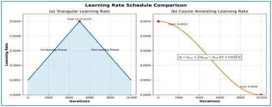
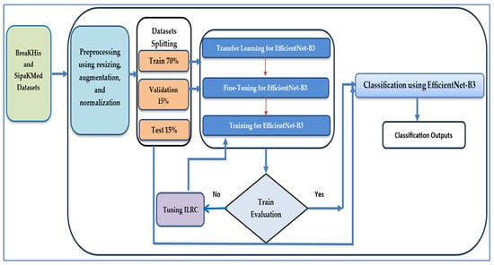
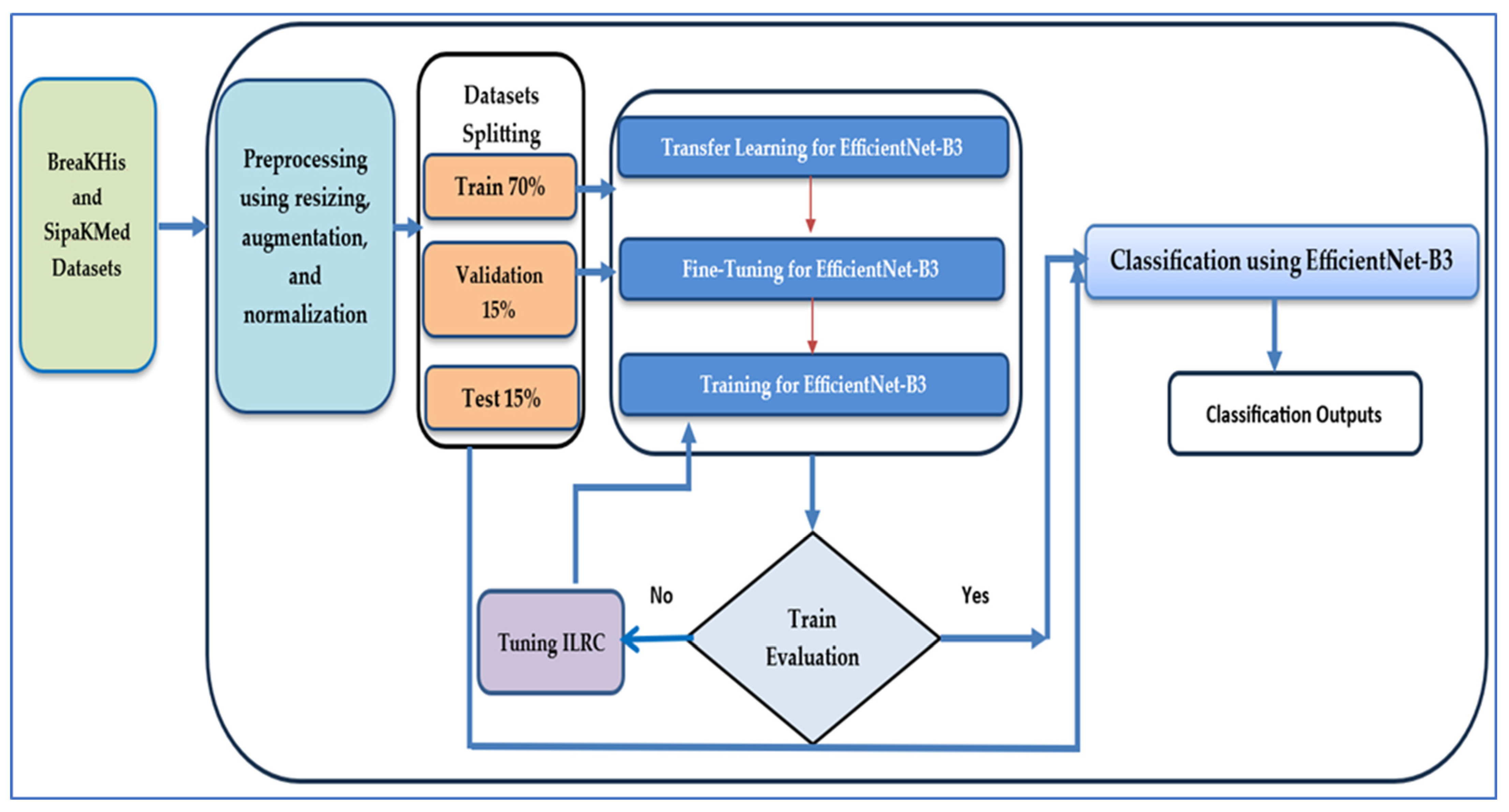
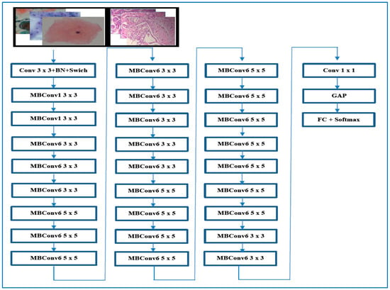
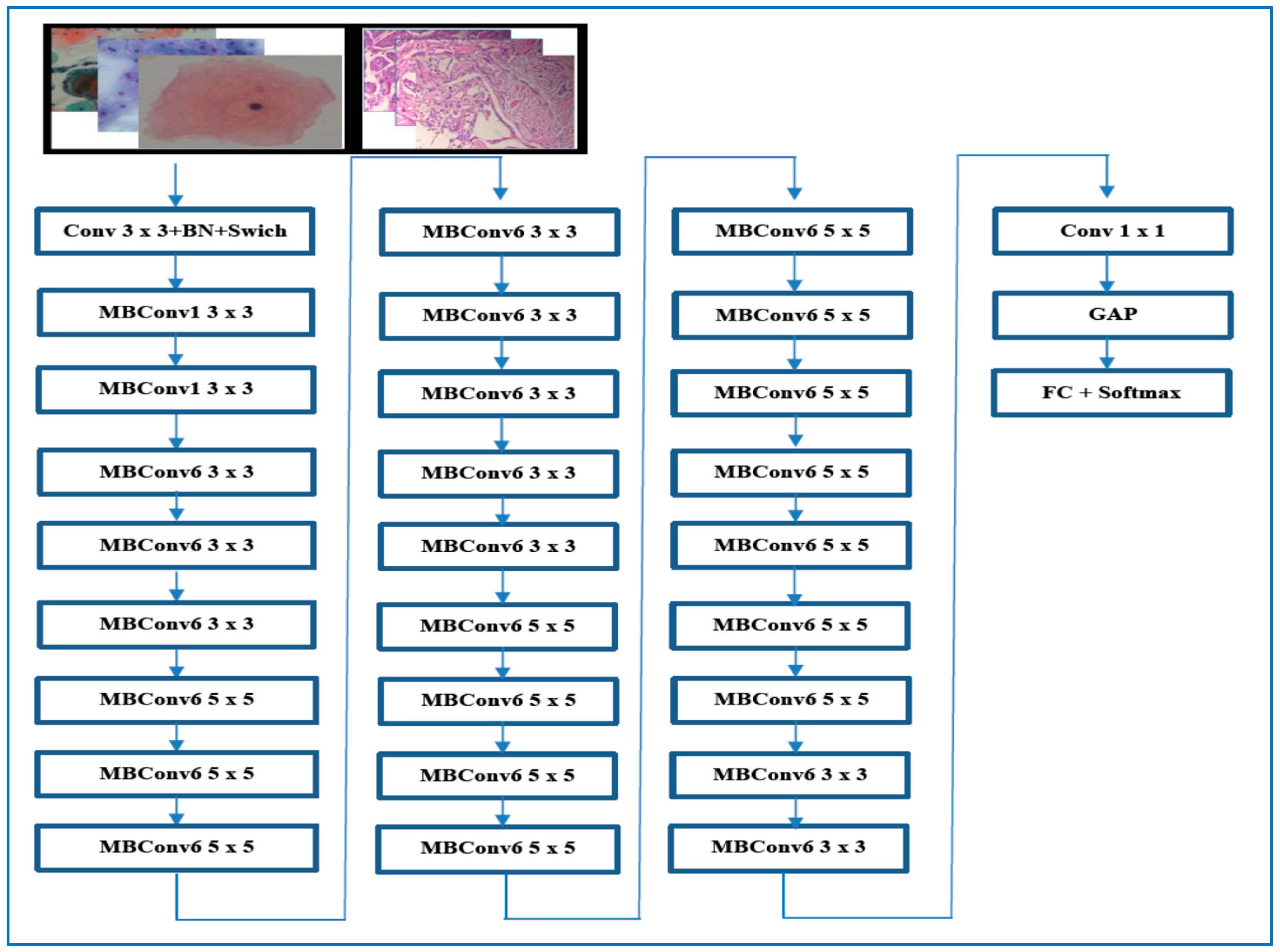
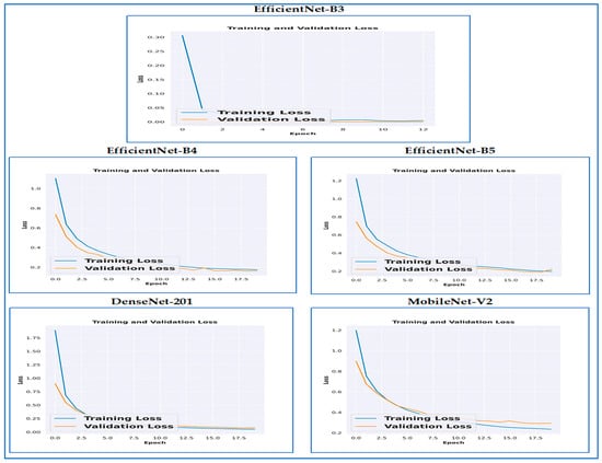
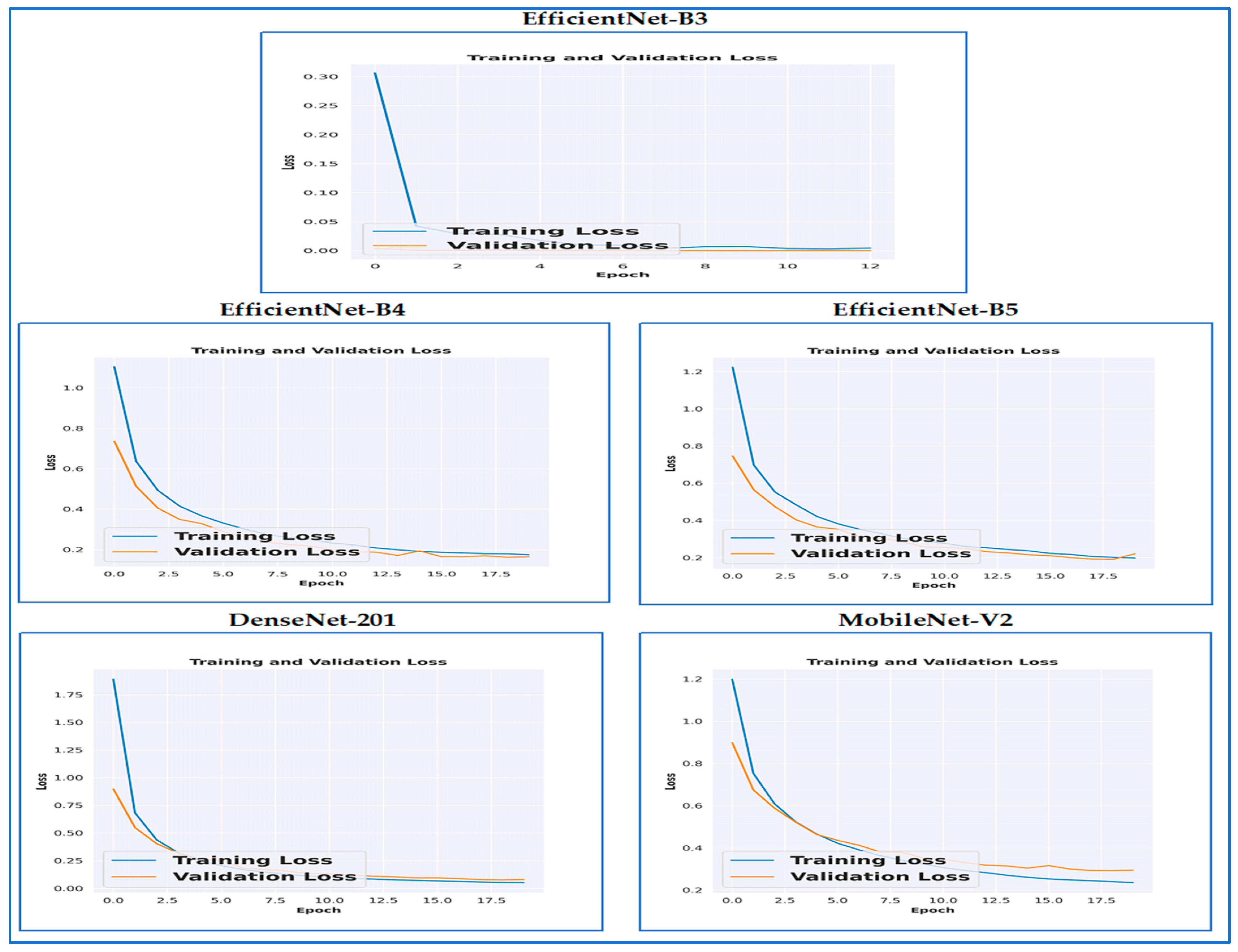
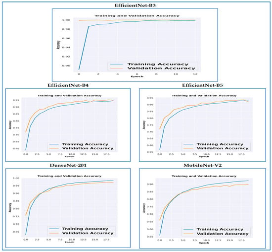
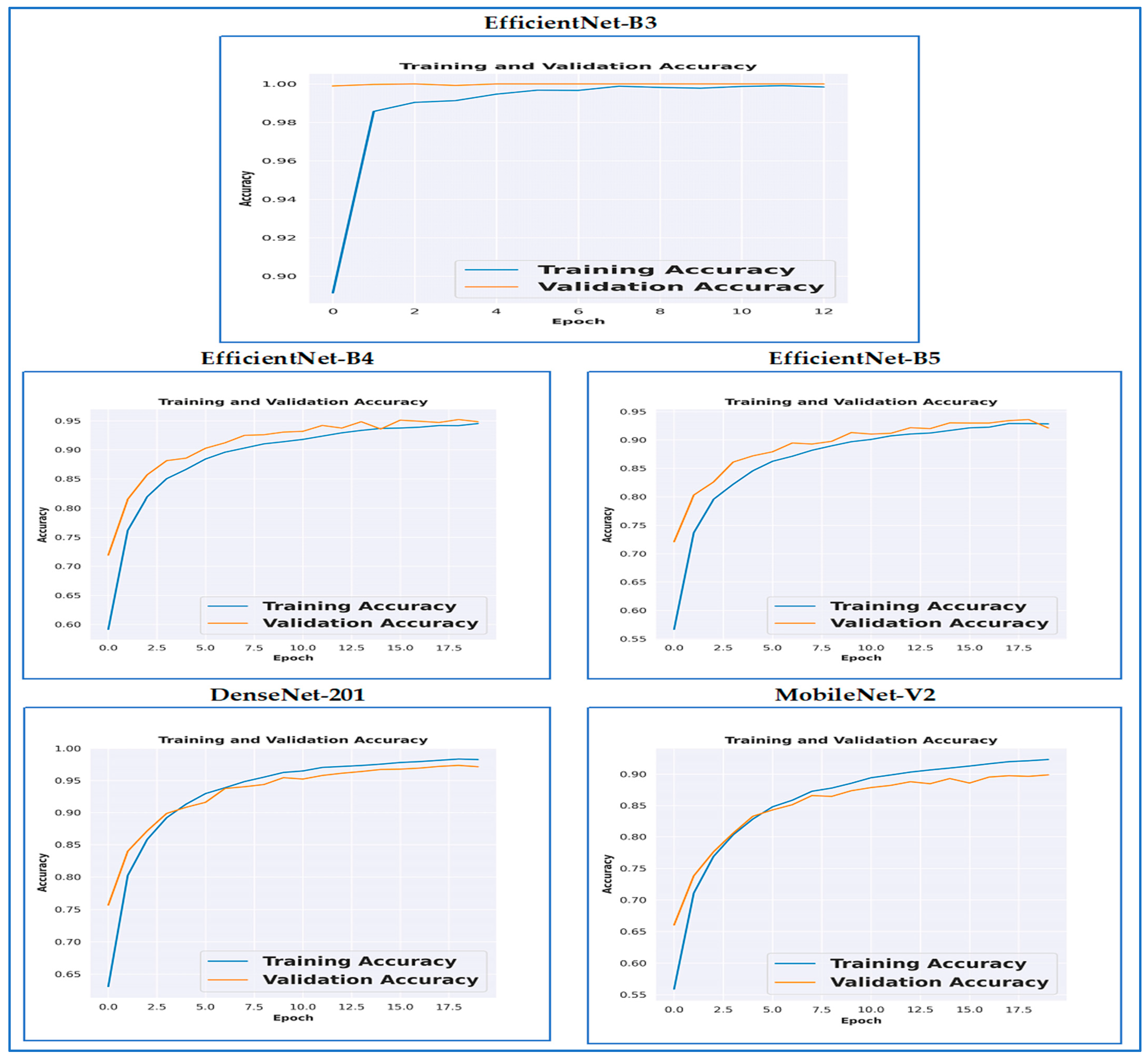
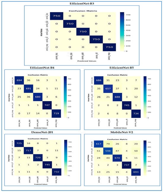
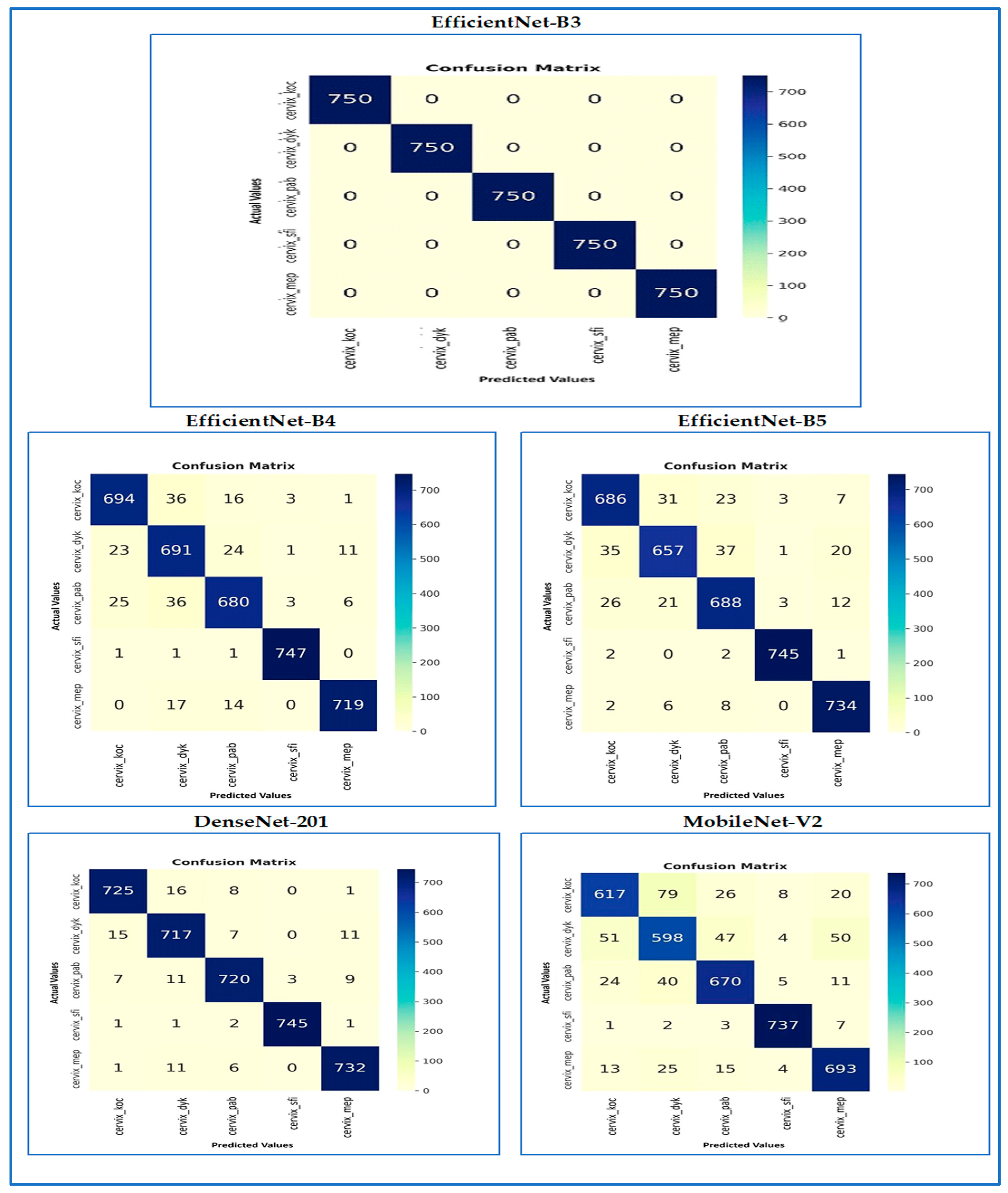
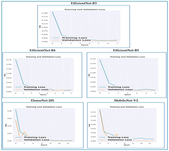
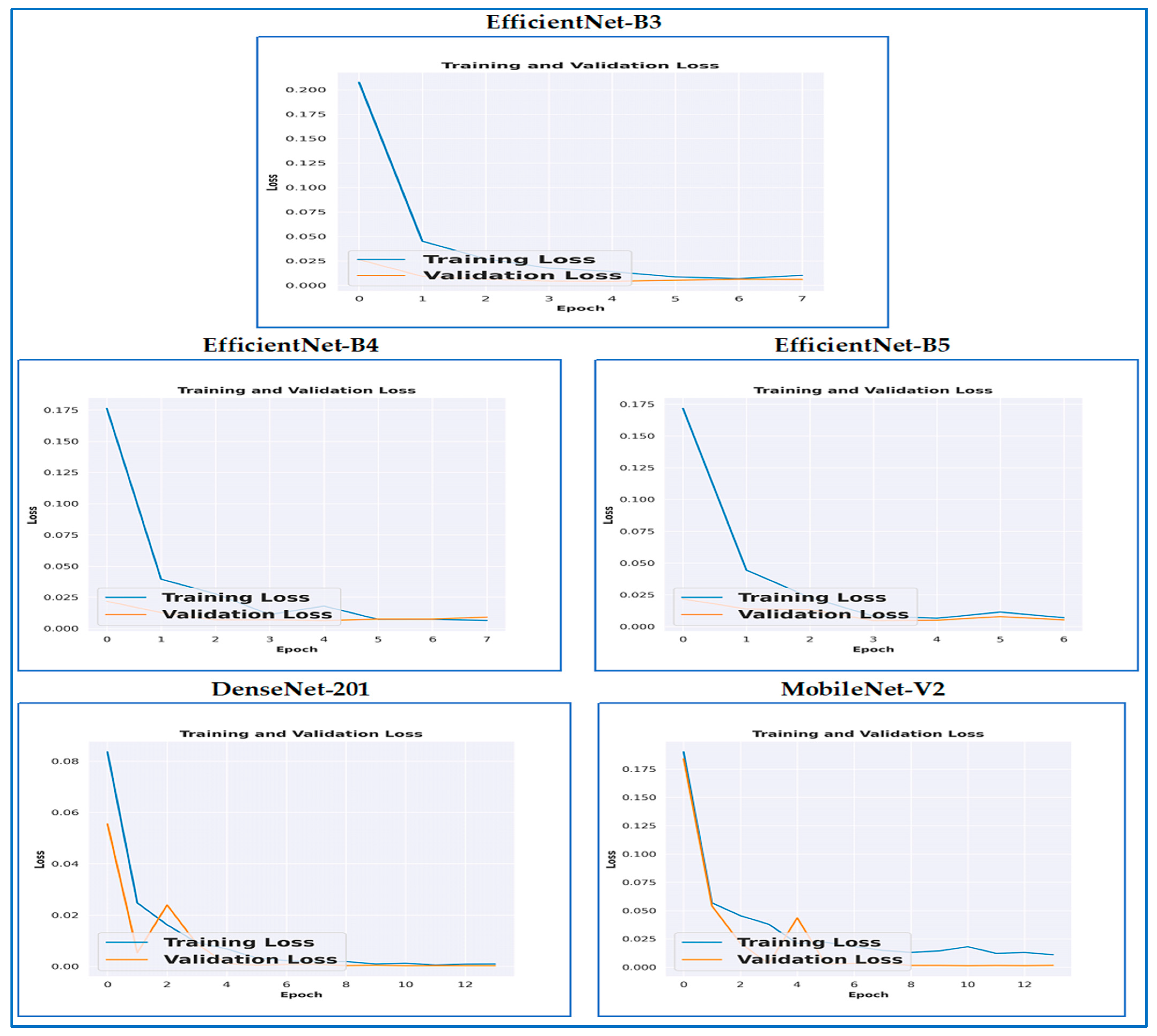
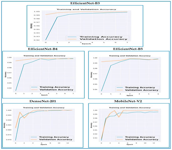
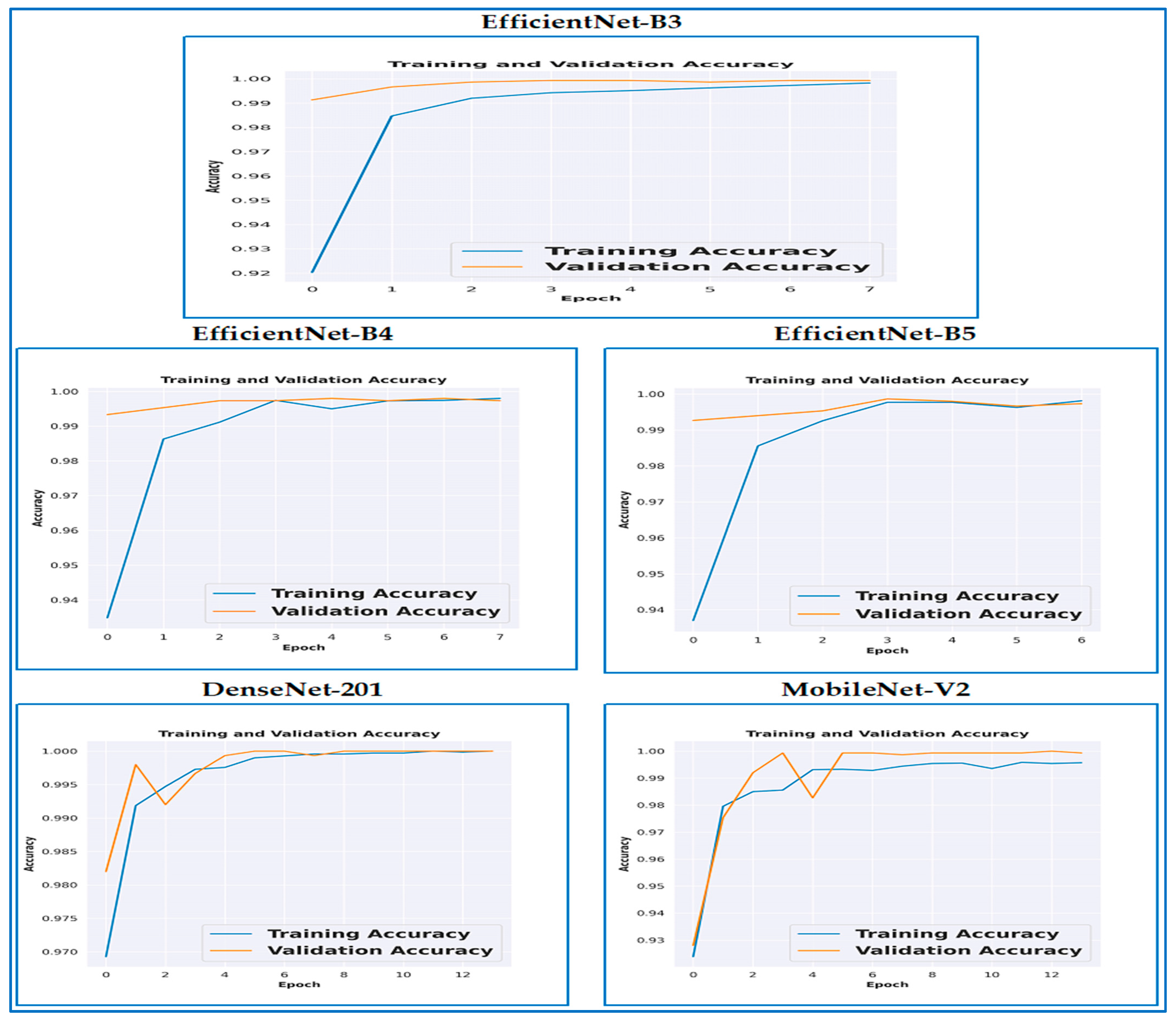
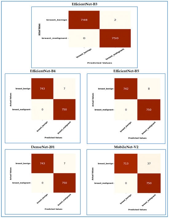
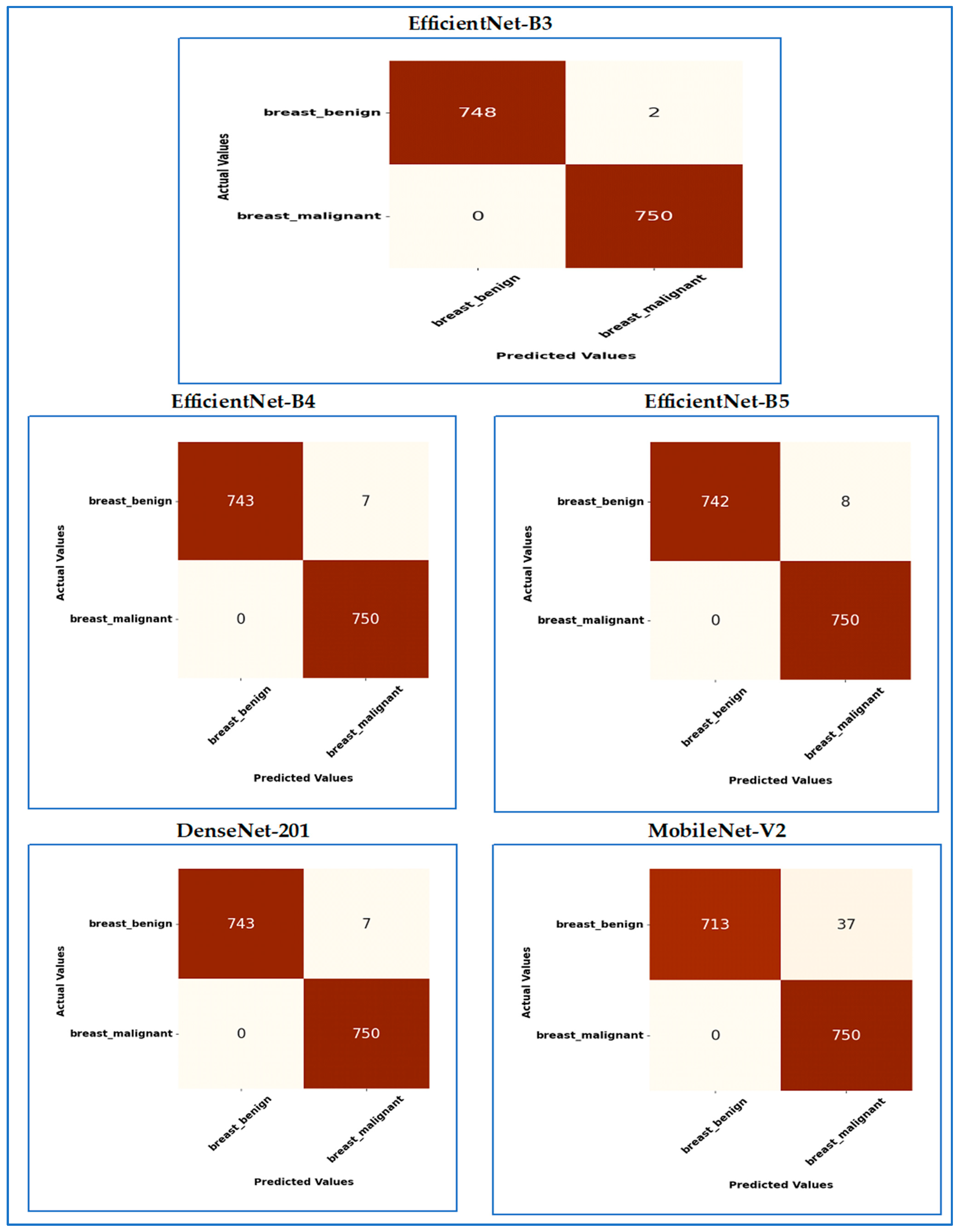
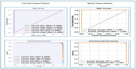
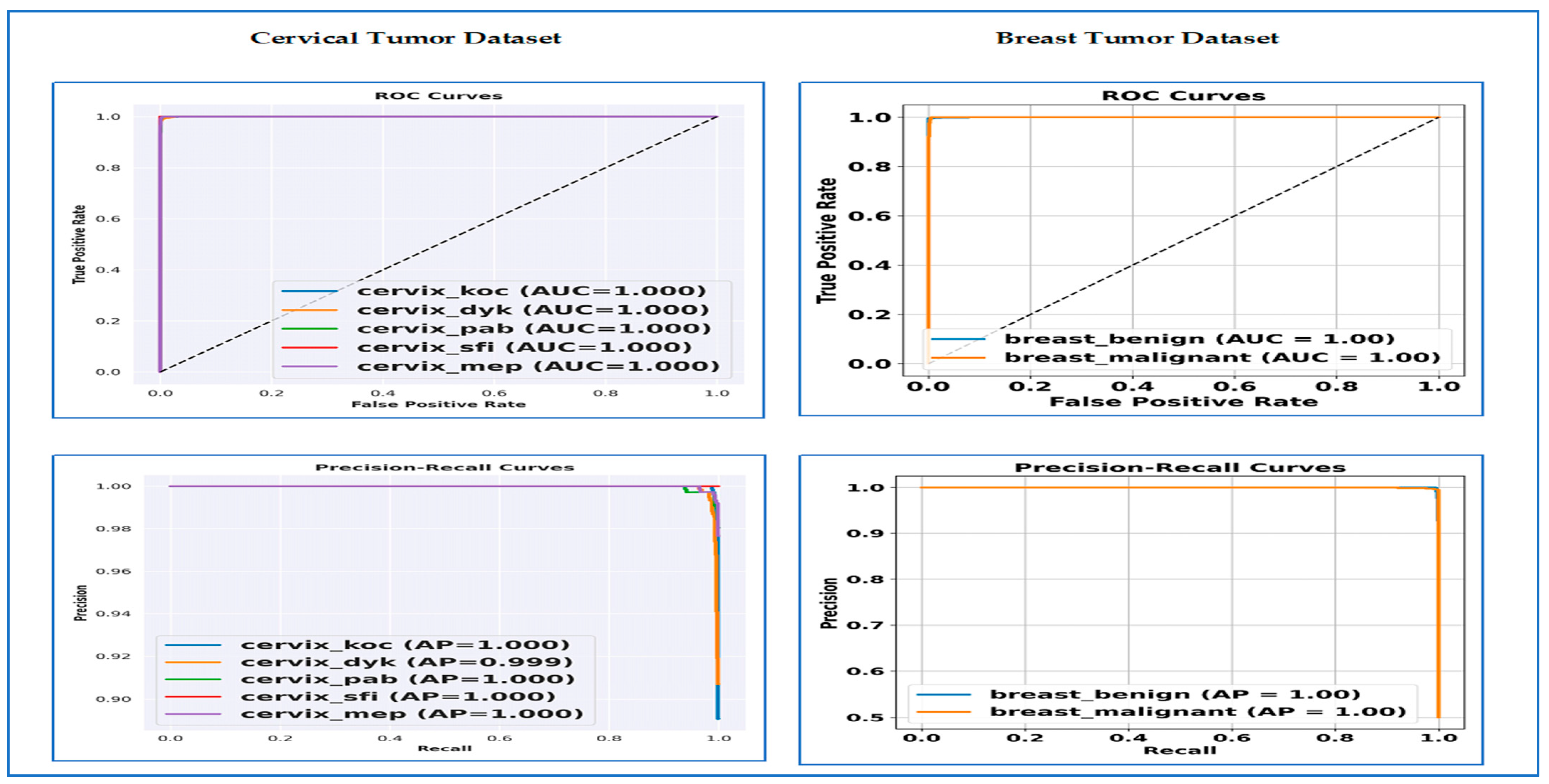

Disclaimer/Publisher’s Note: The statements, opinions and data contained in all publications are solely those of the individual author(s) and contributor(s) and not of MDPI and/or the editor(s). MDPI and/or the editor(s) disclaim responsibility for any injury to people or property resulting from any ideas, methods, instructions or products referred to in the content. |
© 2026 by the authors. Licensee MDPI, Basel, Switzerland. This article is an open access article distributed under the terms and conditions of the Creative Commons Attribution (CC BY) license.