


Abstract
To address the data quality challenges in ship maintenance data, such as high missing rates, anomalous noise, and multi-source heterogeneity, this paper proposes a data quality enhancement method based on a multi-strategy enhanced Harris Hawks Optimization algorithm for optimizing the Kolmogorov–Arnold Stacked Denoising Autoencoder. First, leveraging the Kolmogorov–Arnold theory, the fixed activation functions of the traditional Stacked Denoising Autoencoder are reconstructed into self-learnable B-spline basis functions. Combined with a grid expansion technique, the KASDAE model is constructed, significantly enhancing its capability to represent complex nonlinear features. Second, the Harris Hawks Optimization algorithm is enhanced by incorporating a Logistic–Tent compound chaotic map, an elite hierarchy strategy, and a nonlinear logarithmic decay mechanism. These improvements effectively balance global exploration and local exploitation, thereby increasing the convergence accuracy and stability for hyperparameter optimization. Building on this, an IHHO-KASDAE collaborative cleaning framework is established to achieve the repair of anomalous data and the imputation of missing values. Experimental results on a real-world ship maintenance dataset demonstrate the effectiveness of the proposed method: it achieves an 18.3% reduction in reconstruction mean squared error under a 20% missing rate compared to the best baseline method; attains an F1-score of 0.89 and an AUC value of 0.929 under a 20% anomaly rate; and stabilizes the final fitness value of the IHHO optimizer at 0.0216, which represents improvements of 31.7%, 25.6%, and 12.2% over the Particle Swarm Optimization, Differential Evolution, and the original HHO algorithm, respectively. The proposed method outperforms traditional statistical methods, deep learning models, and other intelligent optimization algorithms in terms of reconstruction accuracy, anomaly detection robustness, and algorithmic convergence stability, thereby providing a high-quality data foundation for subsequent applications such as maintenance cost prediction and fault diagnosis.
1. Introduction
Against the backdrop of intensifying competition over maritime interests, modern vessels are consistently deployed in high-intensity, high-frequency missions while being subjected to the combined effects of multiple extreme operational conditions such as salt spray corrosion, mechanical vibration, and electromagnetic interference. Statistics indicate that maintenance costs already account for 30–50% of the total lifecycle expenses of ships. Furthermore, with increasing levels of intelligentization and frequent switching between multi-mission profiles, maintenance demands are exhibiting exponential growth [1]. Under this backdrop, constructing a high-precision ship maintenance cost prediction model holds significant importance for scientifically formulating maintenance budgets and accurately allocating spare parts resources. However, the practical effectiveness of such prediction models in engineering applications is heavily constrained by the quality of the underlying data. Ship maintenance data encompasses multi-dimensional features such as construction information, performance parameters, and maintenance records. During the processes of acquisition, transmission, and storage, factors such as equipment failures, sensor inaccuracies, and human operations often introduce noise and errors into the data, severely compromising the accuracy and reliability of subsequent analyses [2]. As a key preprocessing technique for enhancing data quality, data cleaning has established relatively mature and effective solutions in various engineering fields, such as power equipment fault prediction [3,4] and wind turbine health management [5]. Building on these cross-domain successes, developing a specialized data cleaning framework tailored to the ship maintenance context has become an urgent requirement. Such a framework is essential for supporting high-precision prediction models and effectively addressing the practical data quality challenges inherent in this domain.
Traditional data cleaning methods primarily rely on statistical theory and classical machine learning algorithms, such as the 3σ rule, regression imputation, cluster analysis, and One-class Support Vector Machines (OC-SVMs). While these approaches demonstrate reasonable usability when handling small-scale, low-dimensional datasets, they often exhibit notable limitations in adaptability and structural suitability when confronted with the high-dimensional, nonlinear, and multi-source heterogeneous nature of ship maintenance data. Specifically, statistical methods based on the identical distribution assumption—such as the 3σ rule [6] and box-plot approach [7]—show high sensitivity to extreme values while demonstrating a limited capability to capture complex nonlinear couplings among multiple parameters. Furthermore, they fail to account for dynamic correlations within the temporal dimension, resulting in the oversight of numerous potential anomalies that are inherently embedded within data structural irregularities. Traditional clustering and classification algorithms—such as K-means [8], DBSCAN [9], and OC-SVM [10]—are highly sensitive to parameter settings. In ship maintenance scenarios characterized by uneven data density distribution or class imbalance, the inherent structural asymmetry of the data often leads to false positives and missed detections. Moreover, their computational complexity increases drastically with data scale, making them inadequate for the efficient cleaning of massive datasets. Furthermore, most traditional methods adopt a strategy of directly removing anomalous data. While this simplifies the operational workflow, it compromises the intrinsic completeness of the dataset, ultimately undermining the reliability of subsequent prediction models.
In recent years, deep learning techniques have brought new breakthroughs to the field of data cleaning. Among various deep models, the Stacked Denoising Autoencoder (SDAE), as a representative unsupervised learning approach, utilizes its symmetric encoder–decoder architecture to learn the underlying distribution patterns of normal data from noisy or incomplete inputs, thereby enabling effective anomaly correction and missing value imputation. Compared to the single-layer Denoising Autoencoder (DAE), the multi-layer stacked structure of SDAE enhances both the level of feature abstraction and robustness to noise. It has achieved promising results in scenarios with relatively stable data patterns, such as power equipment condition monitoring and traffic flow restoration [11]. However, when applied to complex data characteristics like those in ship maintenance, traditional SDAE still exhibits notable limitations in modeling capacity and adaptability. First, these networks typically employ fixed-form activation functions, such as Sigmoid or ReLU, which limits their ability to fit complex, asymmetric data distributions and hinders the effective capture of deep nonlinear coupling relationships among maintenance parameters. Second, most existing SDAE-based repair methods are designed for regularly sampled data or scenarios with low missing rates, whereas ship maintenance data commonly exhibit random missingness and non-uniform sampling. This mismatch leads to insufficient joint modeling capability across temporal and feature dimensions. More critically, the performance of SDAE is highly dependent on key hyperparameters such as the number of hidden nodes and the noise ratio. Current approaches to setting these parameters often rely on empirical assignments or traditional optimization methods like grid search. Although previous studies have attempted to incorporate intelligent optimization algorithms—such as an improved sine-cosine algorithm [12] and an artificial variable beetle antennae search algorithm [13]—for tuning SDAE hyperparameters and have achieved some progress in fields like fault diagnosis, their applicability and effectiveness in the highly asymmetric task of ship maintenance data cleaning remain to be thoroughly investigated.
The No Free Lunch Theorem (NFL) profoundly reveals that in the field of optimization, there exists no universally optimal algorithm suitable for all problems. Its core implication is that the effectiveness of an algorithm is heavily dependent on the alignment between its design and the specific structure and characteristics of the problem at hand. Given the inherent complexities of the ship maintenance data cleaning task, generic optimization algorithms and basic network models often struggle to achieve satisfactory performance. Based on this understanding, this paper proposes a ship maintenance data cleaning method based on a multi-strategy improved Harris Hawks Optimization (IHHO) algorithm for optimizing the Kolmogorov–Arnold SDAE (KASDAE). The core innovations of this method are as follows: (1) To address the inability of the fixed activation functions in traditional SDAE to adapt to complex nonlinear features, the Kolmogorov–Arnold (KA) theory is introduced. This involves reconstructing the network weights into self-learnable B-spline basis functions. Combined with a grid expansion technique, this enables dynamic fine-grained adjustment of the activation functions, significantly enhancing the model’s capability to represent features within multi-source heterogeneous maintenance data. (2) To address the imbalance between exploration and exploitation during hyperparameter optimization, the IHHO algorithm is introduced for optimizing KASDAE parameters, in line with the problem-specific customization principle emphasized by the NFL Theorem. Population diversity is enhanced through a Logistic–Tent compound chaotic map, local search is guided by an elite hierarchy strategy, and the escape energy is dynamically adjusted via a nonlinear decay mechanism based on a logarithmic function. These strategies collectively achieve an effective balance between global exploration and local exploitation. (3) A comprehensive IHHO-KASDAE co-optimization framework is constructed. This framework deeply integrates the data feature-enhanced model with the task-specific improved algorithm, forming a solution capable of adapting to data asymmetry characteristics for ship maintenance data quality enhancement.
2. Related Work
2.1. Overview of Data Cleaning Methods
Data cleaning serves as a core component of data quality management, with its primary task focusing on identifying and rectifying anomalies within datasets. The methodology of data cleaning has evolved from statistical analysis to deep learning, gradually forming a multi-level methodological framework. Throughout this evolution, there has been a continuous focus on exploring the symmetry of data distribution, the symmetry of algorithmic structure, and the symmetry of processing logic.
Statistical analysis-based methods rely on mathematical models of data distribution for anomaly detection, with typical approaches including the 3σ rule, box-plot method, and Grubbs test. These methods offer the advantages of high computational efficiency and straightforward implementation, making them suitable for unidimensional data cleaning tasks that satisfy symmetric distribution assumptions. For instance, Huang et al. [14] applied the 3σ rule to clean water supply network pressure monitoring data, achieving an anomaly recognition accuracy of 89%. However, these methods exhibit a strong dependence on the assumption of symmetric data distribution, leading to limited performance when handling asymmetric data scenarios such as non-Gaussian and multimodal distributions. Research shows that in the context of wind turbine operational data cleaning, the misjudgment rate of the 3σ rule at operational condition switching points can reach 22–35% [15], clearly demonstrating its limitations in dynamic asymmetric systems.
Density-based and clustering-based methods perform anomaly detection by analyzing the spatial distribution characteristics of data points, partially overcoming the constraints of the global symmetric distribution assumption. The DBSCAN algorithm, based on the principle of density reachability, can effectively identify outliers and noise points outside clusters. Cui et al. [16] applied an improved DBSCAN model to process ship AIS data, achieving 92.7% accuracy in anomalous trajectory detection. The LOF algorithm, on the other hand, calculates the local density deviation to accommodate anomaly detection requirements in non-uniform distribution scenarios. Although these methods are capable of handling locally asymmetric data distributions, they remain sensitive to parameter settings and face computational complexity challenges in high-dimensional spaces.
Machine learning-based detection methods primarily fall into two paradigms—supervised and unsupervised learning—each exhibiting distinct characteristics in handling data symmetry. Supervised approaches, such as support vector machines and random forests, rely on labeled data to construct classification boundaries. Han et al. [17] improved the SVM kernel function, achieving an F1-score of 0.91 in industrial process anomaly detection. Unsupervised methods, represented by isolation forest, leverage the isolability of anomalies in feature space for efficient detection. Yang et al. [18] applied this approach to clean SCADA system data of wind turbines, improving computational efficiency by 40% compared to traditional methods. Although these methods demonstrate advantages in constructing symmetric discriminative structures in feature space, supervised learning still faces challenges related to high annotation costs and data imbalance, while unsupervised methods often suffer from limited interpretability of decision logic.
Advanced deep learning-based methods leverage the powerful feature extraction capabilities of neural networks, demonstrating significant advantages in handling high-dimensional and nonlinear data. Autoencoders (AEs) learn essential data characteristics through their encoder–decoder symmetric architecture; Zhao et al. [19] employed an SDAE to process mine ventilation data, maintaining 96% reconstruction accuracy under noisy conditions. Generative models such as GANs and VAEs learn data distributions to generate highly realistic imputations, showing outstanding performance in missing data restoration. Temporal models like LSTM and Transformer excel at capturing time-dependent features; Xu et al. [20] developed a DLSTM model that limited reconstruction error to within 0.5% in turbine data prediction. Although deep learning methods offer breakthrough advantages in feature abstraction, they still face challenges including high computational resource demands and sensitivity to data quality. Achieving an optimal balance between algorithmic efficiency and performance remains a key research focus.
2.2. Application of AE in Data Cleaning
The AE is a specially structured neural network designed to achieve efficient compression and reconstruction of input data through unsupervised learning. In data cleaning tasks, AEs are primarily employed for anomaly detection and noise removal. Their core working principle involves learning a low-dimensional latent representation of normal data and identifying/repairing anomalous points based on reconstruction error. The AE structure, as shown in Figure 1, consists of two main components: an encoder and a decoder. To ensure narrative flow, all symbols related to model parameters, algorithmic variables, and evaluation metrics used in this paper are defined upon their first occurrence. A complete list of notations is provided in Appendix A.
Figure 1.
Basic structure of AE.
The encoder is responsible for mapping the high-dimensional input data to a low-dimensional, dense latent representation . This process can be formally expressed as Equation (1):
where and represent the weight matrix and bias vector of the encoder, respectively, and denotes a nonlinear activation function.
The decoder takes the latent representation from the encoder as input and aims to reconstruct it back into the original high-dimensional space, generating the reconstructed data . This process is formally expressed by Equation (2):
where and are the weight matrix and bias vector of the decoder, respectively, and is the nonlinear activation function employed in the decoder.
The objective of the model training is to optimize all parameters by minimizing the discrepancy between the reconstructed data and the original input . This discrepancy is quantified by a loss function , commonly implemented as the Mean Squared Error (MSE) or cross-entropy. The calculation using MSE is formulated in Equation (3):
After model training is completed, a reconstruction error threshold is established. For any test sample , the anomaly detection procedure is as follows:
Step 1: Feed into the trained AE to obtain the corresponding reconstruction .
Step 2: Calculate the reconstruction error for the sample: .
Step 3: Perform anomaly determination: if , the sample is labeled as an anomaly; otherwise, it is classified as normal.
For detected anomalous data, the normal data distribution patterns learned by the AE can be utilized to replace or correct the abnormal portions. However, standard AEs suffer from structural and functional limitations during data cleaning, such as susceptibility to overfitting and restricted feature representation capability. To address these issues, researchers have proposed various architectural improvements, which can be broadly categorized into three types: AE variants emphasizing enhanced feature learning, generation-oriented architectures, and specialized structures adapted to specific data types.
Feature learning-based AE variants aim to enhance model expressiveness and generalization by incorporating various regularization mechanisms. Sparse Autoencoders (SAEs) enforce sparse activation patterns in the hidden layer through L1 regularization or KL divergence constraints, achieving a balance between interpretability and computational efficiency in feature selection. For example, Yu et al. [21] integrated them with an improved isolation forest for network intrusion detection. Denoising Autoencoders (DAEs) improve robustness against noise corruption by intentionally adding noise to the input and training the network to reconstruct the original clean data. Yin et al. [22] developed a DAE-GRU hybrid model that effectively reduced the impact of asymmetric noise in traffic anomaly detection. Contractive Autoencoders (CAEs) enhance feature stability against minor input variations by penalizing the Jacobian matrix of the encoder output. For complex data scenarios, Stacked Autoencoders (SAEs) enable hierarchical feature extraction through multi-layer network structures. Chen et al. [23] proposed an enhanced SAE-BiLSTM fusion model that demonstrated superior feature abstraction capability in intrusion detection. Xu et al. [24] designed a serial AE that amplifies reconstruction errors of anomalous data through a two-stage reconstruction mechanism, significantly improving sensitivity in time-series anomaly detection.
Generation-oriented AE architectures are designed to learn the underlying distribution of data for sample generation and data imputation, offering unique advantages in handling non-uniform data distributions. Variational Autoencoders (VAEs) employ probabilistic encoding and KL divergence regularization to map inputs to probability distributions in the latent space, demonstrating excellent performance in data generation and anomaly detection tasks. Zhang et al. [25] enhanced the temporal dependency modeling capability of VAE by integrating a BiLSTM network, achieving notable results in time-series anomaly detection. Guo et al. [26] proposed a Memory-Skip VAE that incorporates memory modules and skip connections, effectively improving the accuracy of ship trajectory anomaly detection. Adversarial Autoencoders (AAEs) adopt the concept of generative adversarial networks by using a discriminator to constrain the latent space distribution. Huo et al. [27] optimized AAE training with a mutual information maximization strategy, enhancing semi-supervised anomaly detection performance.
To accommodate the structural characteristics of different data modalities, researchers have developed specialized AE variants aimed at addressing data heterogeneity and structural mismatch in specific domains. Convolutional Autoencoders (CAEs) utilize convolutional and transposed convolutional layers to process high-dimensional grid data such as images; Shen et al. [28] applied CAE to abnormal sound detection in coal mine conveyors, achieving accurate equipment condition monitoring through MFCC feature extraction and reconstruction error analysis. Recurrent Autoencoders (RAEs) employ recurrent neural units like RNN and LSTM to handle sequential data; Sun et al. [29] developed a GRU-DAE model that effectively captured temporal dependencies in power consumption anomaly detection. Graph Autoencoders (GAEs) are designed for graph-structured data; Zhang et al. [30] proposed a traffic flow data repair model based on a self-attention mechanism and GAE, which successfully learned spatiotemporal patterns within urban road network topology. By incorporating domain-specific prior knowledge, these specialized architectures maintain model structural appropriateness while effectively addressing inherent structural and distributional variations across different data types.
2.3. Application of Intelligent Optimization Algorithms in SDAE Optimization
The network architecture of the SDAE comprises an input layer, multiple hidden layers (including encoding and decoding layers), and an output layer, as illustrated in Figure 2. The core concept involves intentionally injecting random noise at the input layer, mapping the noisy input data to a low-dimensional hidden space via the encoder to extract essential features, and then reconstructing the clean original data from the latent features through the decoder.
Figure 2.
Structure of SDAE.
Let the original input data be . A stochastic mapping is first applied to corrupt the input with noise, yielding the noisy data .
The encoding process maps the noisy data to the hidden layer, obtaining the latent feature representation , as expressed in Equation (4):
where is the encoder weight matrix, is the bias vector, and is a nonlinear activation function.
The decoding process reconstructs the latent features into the output , as given by Equation (5):
where and are the decoder weight matrix and bias vector, respectively.
The training objective of the model is to minimize the reconstruction error between the original input and the reconstructed output . The MSE is commonly adopted as the loss function, as defined in Equation (6) [31]:
A single DAE has limited learning capacity, while the SDAE enhances feature representation by stacking multiple DAEs into a deep architecture. The training process consists of two main phases:
Phases 1: Layer-wise unsupervised pre-training. Starting from the bottom DAE, each AE is trained sequentially, with the hidden features output by the preceding encoder serving as input to the subsequent encoder. This enables the model to hierarchically extract abstract features from low-level to high-level representations.
Phases 2: Global supervised fine-tuning. After pre-training all DAEs, the entire network is treated as a multilayer perceptron. Using reconstruction error as the loss function, backpropagation is applied to fine-tune all parameters globally, thereby further optimizing model performance.
During the training phase, the SDAE learns the underlying distribution patterns and intrinsic characteristics of normal data by recovering clean data from actively corrupted, noisy inputs. In the cleaning phase, actual faulty data containing anomalies or missing values is fed into the trained SDAE model. The corresponding cleaning and restoration effect is illustrated in Figure 3.
Figure 3.
Data cleaning and restoration effect of SDAE.
When performing data reconstruction with SDAE, the model utilizes the internal patterns learned from extensive normal data to correct anomalous values that deviate from the normal range, producing reconstructed outputs that align with the overall data distribution. For data samples with missing values, SDAE can accept inputs where missing entries are filled with zeros or random values, and then leverage the complex nonlinear relationships among features through forward propagation to predict the most probable imputations. However, the performance of SDAE in data cleaning and restoration tasks is highly dependent on the configuration of key hyperparameters, such as the number of hidden nodes, sparsity constraints, and the noise ratio. Traditional manual or grid search methods face significant challenges when dealing with such high-dimensional nonconvex hyperparameter optimization problems, including high computational costs and difficulty in obtaining the global optimum. To address these issues, intelligent optimization algorithms have been introduced into the hyperparameter optimization process of SDAE, aiming to achieve exploration and exploitation of the hyperparameter space through their efficient search mechanisms.
In the early stages of research, classical swarm intelligence optimization algorithms were predominantly employed. Zhang et al. [32] achieved notable results in bearing fault diagnosis by optimizing SDAE parameters using an enhanced hybrid strategy combining rat swarm optimization and sparrow search algorithm. Qin et al. [33] utilized a Particle Swarm Optimization (PSO) algorithm to set hyperparameters for an SDAE, enabling high-precision data cleaning in the prediction of driver states within highway tunnels. Narmadha et al. [34] developed a hybrid PSO-AE-LSTM model that employed PSO to tune AE parameters for high-accuracy anomaly classification in network intrusion detection. Furthermore, Han et al. [35] also utilized a PSO algorithm by integrating it with SDAE and a BP neural network for feature extraction from hyperspectral data, which validated the effectiveness of classic optimizers in complex feature learning. On the other hand, probabilistic model-based optimization methods such as Bayesian optimization have also been applied. Peng et al. [36] adopted this approach to systematically optimize the hyperparameters of SDAE, thereby establishing a high-quality data foundation for electric vehicle battery state estimation. These classical algorithms have validated the feasibility of intelligent optimization in SDAE fine-tuning and enhanced model performance in specific tasks. However, they generally suffer from inherent mechanistic deficiencies, such as the tendency of PSO to become trapped in local optima and the rapid decay of population diversity in Differential Evolution (DE). When dealing with nonlinear hyperparameter spaces characterized by complex and rugged landscapes, these methods often struggle to effectively maintain the dynamic balance between global exploration and local exploitation, resulting in insufficient convergence accuracy or premature convergence.
In recent years, a series of novel intelligent optimization algorithms inspired by natural phenomena have been introduced, providing more advanced solutions for the optimization of SDAE. For instance, the Sparrow Search Algorithm (SSA) simulates the foraging and anti-predator behaviors of sparrow populations, balancing search through a finder–follower–sentinel model, and has been demonstrated to possess advantages in convergence speed. Jia et al. [37] fed wavelet time–frequency diagrams into an SDAE model optimized by the SSA for fault diagnosis, achieving excellent results. Liu et al. [38] employed the SSA to tune SDAE parameters, realizing high-precision fault diagnosis for marine diesel engines. The Golden Jackal Optimization (GJO) algorithm, which mimics the cooperative hunting strategy of golden jackals, exhibits strong local escape capability and convergence accuracy. Zhang et al. [39] applied this algorithm to optimize an SDAE, enhancing the fault diagnosis performance for centrifugal pumps. Additionally, other algorithms such as the sine cosine algorithm [12] and the artificial beetle algorithm [13] have also been applied to the optimization of SDAE. In their respective application scenarios, these novel algorithms often demonstrate certain improvements in optimization accuracy, convergence speed, or robustness compared to classical algorithms, thereby advancing the field of data-driven model optimization.
Although the integration of the aforementioned intelligent optimization algorithms with SDAE has achieved progress across multiple fields, their application to the specific task of ship maintenance data cleaning still faces significant adaptation challenges and limitations. Firstly, these algorithms are primarily general-purpose optimizers, and their core search mechanisms are not specifically designed for extracting complex nonlinear coupled features inherent in data cleaning tasks. Secondly, ship maintenance data exhibits strongly asymmetric characteristics, such as high-dimensional heterogeneity and temporal drift, which create an exceptionally complex optimization landscape. This demands that the optimization algorithm possess robust dynamic adaptability and fine-grained search capabilities. Currently, most existing methods are prone to converging to local optima in the later stages of iteration due to the loss of population diversity, or they suffer from limitations in precision within ship maintenance data scenarios because of their fixed energy decay mechanisms, which lack the flexibility to adapt to the varying demands of different optimization phases. More critically, the majority of existing studies treat the optimization algorithm and the deep learning model as two separate components connected in a simple series, lacking a collaborative and adaptive framework. This makes it difficult for the model to dynamically perceive data characteristics and adjust its search strategy during the optimization process, thereby limiting its generalization capability in real-world ship maintenance data environments.
2.4. Limitations of Existing Research
Current studies have provided multiple technical pathways for ship maintenance data cleaning; however, several critical issues remain unresolved when confronting the unique complexities of this domain. First, traditional deep learning methods, such as the SDAE model, rely on fixed-form activation functions. Their static nonlinear mapping capability struggles to adequately capture the complex dynamic couplings among ship maintenance parameters and the distribution shifts under multi-operational condition switching [39]. This structural rigidity limits the model’s capacity to represent the intrinsic data structure, particularly hindering robust extraction of essential features from data with strong noise and high missing rates. Second, most existing research directly applies general-purpose intelligent optimization algorithms to tune SDAE hyperparameters. According to the NFL theorem, the inherent search mechanisms of such algorithms often perform poorly when navigating the specific optimization landscape characteristic of ship maintenance data cleaning. Specifically, they are prone to premature convergence to local optima in the early iterations and suffer from insufficient convergence accuracy later due to loss of population diversity. Although some studies have attempted to introduce newer algorithms like the Golden Jackal Optimization (GJO), their core operations are not specifically designed for the collaborative optimization objectives within this domain [40]. Furthermore, most existing methods treat model design and parameter optimization as separate processes, lacking an end-to-end, collaboratively adaptive framework. This makes it difficult for the models to adapt to the time-varying characteristics and concept drift exhibited by ship maintenance data during long-term monitoring. Consequently, their generalization capability and computational efficiency face significant challenges in practical engineering deployment. Therefore, there is an urgent need to construct a novel framework that deeply integrates advanced representation learning with targeted optimization strategies to address the core challenges in ship maintenance data cleaning.
3. Methodology Design
3.1. KASDAE Model Architecture
Traditional SDAE models employ fixed activation functions, which struggle to adequately capture the strong nonlinearity, multi-source heterogeneity, and multi-condition variability inherent in ship maintenance data. This often leads to significant reconstruction deviations in tasks involving anomaly correction and missing value imputation. To address these limitations, this study reconstructs the conventional SDAE based on the KA theory by incorporating self-adaptive B-spline basis functions as activations. Furthermore, the structure is optimized using grid expansion techniques, thereby establishing a KASDAE model specifically designed for ship maintenance data cleaning.
3.1.1. Theoretical Foundation of KA
The KA theory states that any multivariate continuous function defined on a bounded domain can be decomposed into a finite sum of univariate functions, mathematically expressed as Equation (7):
Here, represent the multi-dimensional input features of ship maintenance data; denotes a univariate basis function responsible for nonlinear mapping of individual features; and is a composite function that integrates the results of multi-feature mappings. Based on this theorem, KASDAE reconstructs the fixed weight matrix of the traditional SDAE into a learnable form of B-spline basis functions, enabling the model to dynamically adapt to the complex distribution of ship maintenance data.
3.1.2. Core Architecture of KASDAE
Traditional SDAE processes data using fixed weight matrices and fixed activation functions, which can be mathematically represented as Equation (8):
where are fixed weight matrices and is a fixed activation function. In contrast, KASDAE reconstructs the weight matrix into learnable B-spline basis functions based on the KA theorem. These basis functions facilitate nonlinear feature mapping and inter-layer transmission. The computational logic for a single layer is given by Equation (9):
where is the layer index; is the input to the -th node in the -th layer; is the number of nodes in the -th layer; is the B-spline basis function connecting the -th and (-th layers; and is the output of the -th node in the (-th layer.
Thus, the overall computation of the KASDAE model can be simplified as Equation (10):
where each represents the transformation defined by the learnable B-spline basis functions at layer .
The detailed architecture of the KASDAE model is illustrated in Figure 4.
Figure 4.
Structure of the KASDAE model.
To enhance the ability of B-spline basis functions to capture detailed characteristics in maintenance data, KASDAE incorporates a grid expansion technique. This technique dynamically adjusts the density of the spline grid, enabling a gradual transition from coarse-grained fitting to fine-grained optimization, thereby effectively mitigating potential overfitting issues caused by an excessive number of initial parameters. The working principle of the grid expansion technique is shown in Figure 5.
Figure 5.
Principle of grid expansion: (a) Coarse-grained B-spline (Initial Training Stage); (b) Fine-grained B-spline (Late Training Stage).
During the initial training phase, the B-spline basis functions are set to order , with the domain defined as (corresponding to the actual value range of a specific feature in ship maintenance data, such as the temperature feature in [−20 °C, 80 °C]). The initial grid width is set as , and the domain is divided into equally spaced subintervals: . To ensure continuity and smoothness of the spline curve at the domain boundaries, the support interval of the basis functions is extended to . At this stage, the coarse-grained B-spline is formed by a linear combination of basis spline functions, expressed mathematically as Equation (11):
where is the weight coefficient of the basis spline function, and is the -th order basis B-spline function.
In the later stage of training, once the model training error converges to a preset threshold, the grid width is expanded to (where ). The domain is then subdivided into finer subintervals: , and the support interval is correspondingly extended to , increasing the number of basis spline functions to . The fine-grained B-spline is given by Equation (12):
where is the weight coefficient of the basis spline under the fine-grained configuration, and is the refined -th order basis B-spline function.
3.1.3. KASDAE Workflow
The feature transformation process of KASDAE is built upon the reconstructed B-spline activation functions and the grid expansion technique, which unfolds in the following three stages:
Stages 1: Input Noise Injection and Data Preprocessing. For each raw ship maintenance data sample , a preset probability is applied to randomly set feature values to zero across all dimensions, producing a noisy input . This procedure simulates random missing entries and noise interference commonly encountered during real-world data acquisition, thereby compelling the model to learn the underlying statistical patterns and inter-feature correlations of the data.
Stages 2: Forward Propagation through Encoder and Decoder. Each layer of the encoder performs the computation defined in Equation (9): first, each input feature undergoes a nonlinear transformation via a set of dedicated learnable B-spline basis functions ; subsequently, all transformed outputs corresponding to the same neuron are linearly weighted and summed to yield the activation value of that neuron. This process is repeated layer-by-layer, ultimately compressing the high-dimensional input into a low-dimensional latent representation . The decoder then takes as input and performs up-sampling layer-by-layer through the same weighted computation using B-spline basis functions, eventually reconstructing an output with the same dimensionality as the original data.
Stages 3: Model Training and Dynamic Grid Expansion. The training objective is to minimize the discrepancy between the reconstructed output and the original input . The MSE is adopted as the loss function, as given in Equation (13):
where denotes the true value of the -th feature in the -th sample, is the corresponding reconstructed value, is the total number of samples, and is the feature dimensionality.
The training process is optimized using mini-batch stochastic gradient descent. Both the control point coefficients of the B-spline basis functions and the linear weights between network layers are treated as trainable parameters and updated jointly via backpropagation. In the initial training phase, B-splines defined with a relatively coarse grid density are employed, allowing the model to rapidly capture the main trends of the data. When the training loss converges and enters a plateau, a grid expansion operation is triggered: the grid density of the B-splines is increased to , and the newly added control point parameters are initialized. The model then continues training on the refined grid to capture more subtle nonlinear patterns in the data. The entire training procedure uses the Adam optimizer, and an early-stopping strategy based on a validation set can be applied to prevent overfitting.
Through the above procedure, KASDAE ultimately learns a complex nonlinear mapping from noisy data to clean data. The key lies in its use of learnable B-splines and a dynamic grid structure, which enable the model to adapt to the inherent complexity of ship maintenance data, thereby achieving superior reconstruction and repair capabilities. The restoration effect is demonstrated using temperature data reconstruction as an example, as illustrated in Figure 6.
Figure 6.
Temperature data reconstruction curves: (a) Temperature data with anomalies and gaps; (b) KASDAE temperature data reconstruction.
3.2. Multi-Strategy IHHO Algorithm
The performance of the KASDAE model is highly dependent on its hyperparameter configuration, which constitutes a high-dimensional, nonconvex, and computationally intensive optimization problem. Although the objective function appears relatively straightforward, the training dynamics of deep neural networks, result in a loss landscape characterized by numerous local optima and flat regions. Commercial optimizers are primarily designed for differentiable convex optimization or combinatorial problems with well-defined structures; their efficiency and global search capability are often limited in such complex black-box function optimization. In contrast, metaheuristic algorithms do not rely on gradient information and excel in global exploration within high-dimensional spaces, making them more suitable for this type of problem. Among numerous nature-inspired optimization algorithms, the HHO algorithm shows considerable potential due to its clear mechanism that mimics the predatory behaviors across different exploration and exploitation phases. It achieves an adaptive transition between search phases through an escape energy parameter, offering an inherent advantage in balancing global exploration and local exploitation. However, the HHO algorithm employs a linear energy decay mechanism. This fixed strategy struggles to meet the dynamic requirements for search behavior during different stages of KASDAE hyperparameter optimization, often leading to insufficient convergence accuracy or entrapment in local optima. Therefore, building upon the HHO framework, this paper introduces a multi-strategy enhancement mechanism to develop the IHHO algorithm. The aim is to enhance its dynamic adaptability and search efficiency when tackling complex optimization problems, thereby achieving more precise and stable optimization of KASDAE hyperparameters.
3.2.1. Fundamentals of HHO Algorithm
The HHO algorithm is selected as the foundation for enhancement in this work for the following reasons. First, the algorithm adaptively regulates exploration and exploitation behaviors via an energy factor. This mechanism is clear and easily amenable to targeted improvements, allowing it to better adapt to the optimization landscape of specific problems. Second, compared with other classical algorithms, HHO has demonstrated competitive convergence accuracy and robustness across a variety of complex benchmark problems. Inspired by the cooperative hunting behavior of Harris’s hawks, its search strategy exhibits strong performance in solving high-dimensional nonlinear problems [41]. In the HHO algorithm, each candidate solution to the optimization problem is represented as the position of a Harris’s hawk. The core of the algorithm simulates the complete process from prey discovery to cooperative siege by the hawk group. It utilizes the prey’s escape energy, denoted as , to dynamically control a smooth transition from global exploration to local exploitation.
In HHO, the population consists of hawk individuals, where each individual’s position represents a candidate solution in the search space. The algorithm iteratively updates the positions of the hawks to progressively approach the global optimum. Its core mechanism is described as follows:
1. Escape Energy Mechanism. The escape energy is a key parameter that governs the transition from global exploration to local exploitation, defined by Equation (14):
where denotes the initial energy, which follows a uniform distribution over the interval [−1, 1]; is the current iteration number; and is the maximum number of iterations. The absolute value reflects the physical state of the prey. Based on the threshold of , the search stage is determined:
(1) When , the prey is considered energetic and highly motivated to escape. The algorithm operates in the global exploration phase, where the hawk group broadly searches the solution space to locate potential prey regions.
(2) When , the prey’s energy declines, and the algorithm enters the local exploitation phase, during which the hawks perform refined search around the already identified potential optimal solutions.
2. Exploration Phase. During the exploration phase, the hawk population updates its positions using one of two equally probable strategies to conduct a broad search of the solution space. The position update rule is given by Equation (15):
Here, denotes the position of a randomly selected individual from the current population, represents the current best solution, and is the average position of the hawk population. The coefficients , , , , and are random numbers uniformly distributed in [0, 1], while and are the lower and upper bounds of the search space, respectively.
3. Exploitation Phase. During the exploitation phase, the algorithm employs four distinct besiege strategies based on the escape energy and a random number , simulating the cooperative hunting behavior of the hawk group. A threshold of 0.5 is used to further differentiate the intensity of strategies within this phase, aiming to balance convergence speed and solution diversity: ≥ 0.5 indicates that the prey still retains some energy, corresponding to relatively gentle surrounding tactics; whereas < 0.5 suggests the prey is fatigued, warranting more aggressive besiege maneuvers.
(1) Soft Besiege. When ≥ 0.5 and ≥ 0.5, a soft besiege strategy is adopted. The position update is given by Equation (16):
where represents the vector difference between the prey position and the current Harris hawk’s position; is used to simulate the random jumping behavior of the prey during escape, with being a random number within [0,1]. The introduction of increases the stochasticity of local search, helping to maintain a certain level of population diversity during the exploitation phase. This design originates from the original HHO algorithm’s simulation of predator–prey escape interactions.
(2) Hard Besiege. When < 0.5 and ≥ 0.5, a hard besiege strategy is employed. The position update is defined as Equation (17):
(3) Soft Besiege with Progressive Rapid Dives. When ≥ 0.5 and < 0.5, a soft besiege strategy combined with progressive rapid dives based on Lévy flight is adopted. The position update is expressed as Equation (18):
where denotes the objective function value for the minimization problem, and and are computed as Equation (19):
Here, is the dimensionality of the problem; is a random vector with each component drawn uniformly from (0,1); and represents the Lévy flight function, calculated as Equation (20):
In the above expression, and are random numbers within (0,1), and is a predefined constant.
(4) Hard Besiege with Progressive Rapid Dives. When < 0.5 and < 0.5, a hard besiege strategy combined with progressive rapid dives is applied. In this case, and are defined as Equation (21):
3.2.2. Multi-Strategy Improvement Design
While the HHO algorithm demonstrates strong performance on numerous benchmark problems, it exhibits notable limitations when applied to hyperparameter optimization tasks with complex characteristics, such as ship maintenance data cleaning. These limitations primarily manifest in the following three aspects. First, the algorithm relies on random initialization to generate the initial population, which may fail to ensure an even distribution and sufficient diversity of individuals across the complex search space, potentially compromising the efficiency of global exploration. Second, its core escape energy update mechanism follows a linear decay pattern. This rigid strategy does not align well with the dynamic needs of the optimization process, resulting in an insufficiently flexible transition between the exploration and exploitation phases. Finally, during later iterations, the population tends to converge around the current best solution. The algorithm lacks effective mechanisms to guide individuals away from local optima or to enhance the precision of local search, thereby constraining its ultimate convergence performance.
To address these issues, this study introduces three targeted enhancements to the HHO algorithm, refining it across three key dimensions: population initialization, search guidance, and energy regulation [42]. First, a Logistic–Tent compound chaotic map is employed for population initialization. This is designed to improve the uniformity and ergodicity of the initial solution distribution in the search space, laying a solid foundation for global exploration. Second, an elite hierarchy strategy is designed, guiding ordinary individuals to learn from elite individuals. This balances the algorithm’s global exploration capability with the intensity of local exploitation. Third, the linear energy decay mechanism is replaced by a nonlinear decay strategy based on a logarithmic function. This allows the algorithm to adjust its search behavior more smoothly and adaptively across different optimization stages. These three enhancements work synergistically, forming the IHHO algorithm proposed in this study.
1. Population Initialization via Logistic–Tent Compound Chaotic Map. To overcome the uneven population distribution caused by traditional random initialization, a Logistic–Tent compound chaotic map is introduced to generate the initial population. This map combines the ergodicity of the Logistic map with the uniform distribution characteristics of the Tent map. The chaotic sequence is generated by the following iterative formula, mathematically expressed as Equation (22):
Here, is a control parameter; denotes the modulo operation; represents the current chaotic state value, which is used as the initial position of an individual in the population; and is the next state value computed via the mapping, employed to generate new individual positions. This strategy constructs an initial population with high diversity and uniform distribution during the initialization phase, thereby effectively preventing premature convergence caused by an uneven initial distribution.
2. Elite Hierarchy Strategy. To balance the algorithm’s global exploration and local exploitation capabilities, an elite hierarchy strategy based on fitness ranking is introduced. In each iteration, the top 10% of individuals with the best fitness values are selected to form an elite group . The remaining individuals then move toward the elite individuals according to the following position update formula given in Equation (23):
Here, is a guiding individual randomly chosen from the elite group; and are control parameters within the interval [0, 1]. By leveraging the guidance of elite individuals, this mechanism enhances local search capability while preserving population diversity, thereby achieving a dynamic balance between the exploration and exploitation phases. This helps mitigate the issue of insufficient convergence accuracy in the later iterations of the HHO algorithm, which often results from declining population diversity.
3. Nonlinear Decay Strategy Based on Logarithmic Function. To address the limitation of the traditional HHO’s linear energy decay mechanism in adapting to complex optimization scenarios, a nonlinear escape energy update mechanism based on a logarithmic function is proposed. Its calculation formula is given by Equation (24):
Here, and represent the initial and final values of the energy, respectively; is the current iteration number; and is the maximum number of iterations. This strategy maintains a high energy level in the early iterations to promote global exploration, while allowing a gradual decay in the later stages to intensify local exploitation. This facilitates a smooth transition in the algorithm’s search behavior, effectively coordinating the requirements across different optimization phases. A comparison of the escape energy curves is illustrated in Figure 7.
Figure 7.
Escape energy comparison.
In summary, the three core enhancements made to the HHO algorithm in this study are as follows. Firstly, the Logistic–Tent compound chaotic map is primarily responsible for generating an initial population with greater uniformity and ergodicity at the start of the optimization process, establishing a diverse foundation for global exploration. Secondly, the elite hierarchy strategy dynamically balances the algorithm’s global exploration capability and local exploitation intensity by guiding ordinary individuals to learn from elite ones during iteration, thereby preventing premature convergence and improving local search precision. Finally, the nonlinear decay strategy based on a logarithmic function replaces the original linear mechanism, enabling a smoother variation in escape energy throughout the iterative process. This allows more precise control over the transition rhythm from global exploration to local exploitation. These three enhancements act on different key stages of the algorithm workflow. Functionally complementary, they together constitute a synergistically reinforced optimization framework.
3.2.3. IHHO Algorithm Flow
The complete procedure of the IHHO algorithm for KASDAE hyperparameter optimization is illustrated in Figure 8, with the detailed steps as follows:
Figure 8.
IHHO algorithm process.
Step 1: Parameter initialization and search space definition. Set the basic operational parameters of the IHHO algorithm according to the problem scale. These include the population size , the maximum number of iterations , the chaos control parameter , the initial and final values of escape energy and , and the elite ratio = 10%. Simultaneously, define the optimization search space for the KASDAE hyperparameters, encompassing the number of encoder nodes , the number of decoder nodes , the initial B-spline grid density , the input zeroing ratio , and the lower and upper bounds for the learning rate .
Step 2: Population initialization based on chaotic mapping. To address the non-uniformity inherent in random initialization, a Logistic–Tent compound chaotic map is employed to generate a chaotic sequence of length . This sequence is then sequentially reshaped into vectors of dimension . Each vector is linearly mapped to the actual hyperparameter search space using the lower and upper bounds defined in Step 1, thereby obtaining an initial population with favorable ergodicity.
Step 3: Fitness evaluation. For each individual in the population, its position vector is first decoded into a specific set of KASDAE hyperparameters. Using this parameter set, a KASDAE model is initialized and trained on a fixed training set. Training is performed with mini-batch gradient descent for a sufficient number of epochs to ensure preliminary convergence of the model. After training, the reconstruction mean squared error of the model on the validation set is computed and taken as the fitness of that individual, as given by Equation (25):
where is the original data value from the validation set and denotes the reconstructed value produced by the KASDAE model configured with hyperparameters . A smaller fitness value indicates better performance of the corresponding hyperparameter set.
Step 4: Elite group selection and global best solution recording. After evaluating the fitness of all individuals, the population is sorted in ascending order of fitness values. The top individuals are selected to form the elite group . Simultaneously, the global best position is recorded.
Step 5: Nonlinear update of escape energy. Based on the current iteration count , the escape energy is updated using the logarithmic nonlinear decay strategy defined in Equation (24). This strategy ensures that decays relatively slowly in the early iterations to maintain exploration, while decaying gently in the later iterations to facilitate deep exploitation.
Step 6: Population position update integrated with elite guidance. Based on the updated value of , the algorithm phase is determined. If ≥ 1, global exploration is performed and positions are updated according to Equation (15). If < 1, the algorithm enters the local exploitation phase, where one of the four besiege strategies (Equations (16)–(21)) is selected for position update according to the values of and a random number . A key refinement in this step is the introduction of an elite guidance mechanism during position updating in the exploitation phase. For non-elite individuals, their updates are partially influenced by an elite individual randomly chosen from the elite group . The specific guidance is implemented as shown in Equation (23).
Step 7: Iteration termination and optimal solution output. Check the termination criteria: whether the maximum iteration count has been reached, or whether the improvement of the global best fitness over consecutive iterations falls below a preset threshold . If either condition is satisfied, the iteration terminates and the historically recorded global best hyperparameter set is output. Otherwise, return to Step 3 to proceed with the next iteration.
3.3. IHHO-KASDAE Data Cleaning Process
The IHHO-KASDAE collaborative cleaning framework represents a systematic solution that deeply integrates targeted optimization with adaptive modeling. Its core idea is to employ the IHHO algorithm to automatically search for the optimal KASDAE configuration that matches the complex characteristics of the data, thereby achieving high-precision restoration of mixed quality issues in ship maintenance data. The complete system workflow is illustrated in Figure 9; the specific steps and the design considerations behind them are as follows:
Figure 9.
Schematic of the IHHO-KASDAE data cleaning process.
Step 1: Data Preprocessing and Normalized Partitioning. The raw dataset is preprocessed by applying min–max normalization, which linearly scales each feature to the range [0, 1] according to Equation (26):
where is the original feature value, and and are the minimum and maximum values of that feature in the training set, respectively.
For any inherent missing values present in the data, temporary zero-filling is applied during preprocessing. This preserves the structural integrity of the data matrix, while the model will learn through training to distinguish such placeholder zeros from genuine valid data. The normalized complete dataset is then partitioned into a training set and a test set according to a predefined ratio, ensuring that the partitioning reflects the overall data distribution to avoid bias.
Step 2: Adaptive Hyperparameter Optimization Driven by IHHO. The key parameters governing the model capacity and behavior of KASDAE—including the number of nodes in the encoding and decoding layers (), the initial B-spline grid density , the input noise ratio , and the learning rate —are formulated as a high-dimensional continuous optimization problem. Leveraging its enhanced capabilities in maintaining population diversity and balancing exploration versus exploitation, the IHHO algorithm is employed to automatically search for the optimal solution to this problem. The fitness function is defined as the reconstruction mean squared error of KASDAE on an independent validation subset, which directs the optimization process explicitly toward improving the model’s generalization and repair performance. Through this step, the model architecture is no longer predetermined but instead evolves into a data-driven optimal configuration.
Step 3: Deep Training of KASDAE Based on the Optimal Configuration. The optimal hyperparameter set is used to configure the corresponding KASDAE network architecture. Subsequently, this model undergoes comprehensive end-to-end training using the complete training set . During training, leveraging its learnable B-spline basis functions and dynamic grid expansion mechanism, KASDAE adaptively captures the complex nonlinear patterns and local intricacies within the data. By minimizing the reconstruction loss, the encoder progressively learns a compact, low-dimensional manifold representation of the ship maintenance data in its clean state, while the decoder masters the ability to reconstruct complete and normalized data from this manifold.
Step 4: Data Cleaning and Reconstruction Repair Based on Model Knowledge. The actual data containing quality issues such as anomalies and missing values, denoted as , is fed into the trained KASDAE model. The forward propagation process of the model essentially projects the problematic data onto the learned manifold of normal data and performs reconstruction. Since anomalies deviate from this normal manifold, they incur larger reconstruction errors. The decoder, constrained by the manifold structure, generates outputs that reconstruct these points into the normal value range, thereby achieving correction. Temporary zero-fill values in the input are treated as information to be inferred during manifold projection. Leveraging the learned complex nonlinear relationships among features, the model infers the optimal imputation values that best conform to the overall data distribution from the available partial information. Ultimately, the model outputs a reconstructed, quality-enhanced dataset .
Step 5: Data Post-Processing and Application Output. The cleaned and repaired normalized data, , undergoes reverse normalization to restore its original physical dimensions and numerical scale. This yields the final high-quality dataset , which is directly applicable to downstream analytical tasks. The output of this framework preserves the intrinsic feature correlations and statistical properties of the original data through a data-driven repair process, thereby establishing a reliable data foundation for subsequent advanced analyses such as maintenance cost prediction.
4. Experiments and Analysis of Results
4.1. Experimental Setup
4.1.1. Dataset and Preprocessing
The experimental data used in this study were collected during a six-month field investigation, comprising actual ship maintenance records accumulated by seven major shipyards between 2010 and 2023. After performing completeness verification and logical consistency cleaning on the raw data, a final dataset containing 673 valid samples was constructed. Each sample includes 11 key engineering features that comprehensively describe the ship’s basic attributes, performance status, and maintenance process. These features are: construction cost, displacement, ship length, ship width, draft depth, maximum speed, main engine power, service length at the time of maintenance, maintenance duration, actual labor hours, and total maintenance cost. This dataset authentically reflects the multi-source and heterogeneous characteristics inherent in ship maintenance activities. To meet the input requirements of deep learning models, min–max normalization, as described in Equation (26), was applied to standardize features with different units, linearly mapping each feature value to the [0, 1] interval. The entire dataset was then divided into a training set and a test set in a 7:3 ratio using stratified random sampling. This approach ensured that the distribution proportions of different ship types, tonnage classes, and maintenance scales remained approximately consistent across both sets.
4.1.2. Evaluation Metrics
To comprehensively evaluate the overall performance of different data cleaning methods, a multi-dimensional evaluation index system was established, covering aspects such as reconstruction accuracy, anomaly detection, missing value imputation, algorithm efficiency, comprehensive error, and the basis for statistical testing.
1. Reconstruction Accuracy Metrics. As core indicators for measuring the ability of a cleaning model to recover the original clean data, the Root Mean Square Error (RMSE) and Mean Absolute Error (MAE) were adopted. Their calculation formulas are shown in Equation (27):
where is the original true value, is the value reconstructed by the model, is the number of samples, and is the feature dimensionality.
2. Comprehensive Error Metrics. To provide a more comprehensive error analysis, two additional metrics are introduced: the Sum of Squared Error (SSE) and the Mean Relative Error (MRE). SSE reflects the cumulative scale of the total error, while MRE measures the magnitude of the error relative to the true value. Their calculation formulas are given in Equation (28):
Here, is a very small constant introduced to avoid division by zero.
3. Anomaly Detection Performance Metrics. To evaluate the effectiveness of the methods in identifying anomalous data points, Precision, Recall, and F1-Score are introduced as evaluation metrics. Their calculations are based on the outcomes of anomaly detection: True Positives (TP), False Positives (FP), and False Negatives (FN). The corresponding formulas are provided in Equation (29):
4. Missing Value Imputation Performance Metric. For the missing value imputation task, the Imputation Error (IE) is used for evaluation, defined as the MSE between the values imputed by the model and the corresponding ground truth values. The calculation formula is given by Equation (30):
where is the total number of artificially introduced missing values, is the masked true value, and is the value imputed by the model.
5. Algorithm Efficiency Metrics. To compare the efficiency of different optimization algorithms and cleaning models, two key metrics were adopted: first, the convergence generation, which refers to the minimum number of iterations required for the optimization algorithm to satisfy the preset convergence criterion; second, the computation time, defined as the total CPU/GPU time consumed by the model to complete the entire training process or to clean a specified dataset under identical hardware conditions.
6. Basis for Statistical Testing and Multi-Criteria Decision Making. To ensure the statistical rigor of performance comparisons, the non-parametric Wilcoxon signed-rank test was employed to analyze the significance of performance differences between two methods. For the comprehensive ranking of multiple algorithms, the Friedman test was utilized. Furthermore, to facilitate integrated trade-offs and decision-making among multiple potentially conflicting evaluation criteria, the theoretical framework of Multi-Criteria Decision Making (MCDM) methods was introduced in the subsequent comprehensive analysis, providing more engineering-practical guidance for algorithm selection.
4.1.3. Comparative Methods and Parameter Configuration
To systematically validate the performance of the proposed IHHO-KASDAE method in ship maintenance data cleaning tasks, a multi-level comparative framework was constructed, encompassing representative approaches from diverse technical paradigms including traditional statistics, classical machine learning, deep learning, and their integration with optimization algorithms. All experiments were conducted under the same Python environment utilizing mainstream libraries such as Scikit-learn 1.3.0 and PyTorch 2.1.0, and were performed using an identical dataset with the same training-test split to ensure the fairness of the comparisons.
Within the domains of traditional statistics and classical machine learning, the 3σ Rule, the Boxplot method, Isolation Forest, and OCSVM were selected as baselines, representing cleaning approaches based on distribution assumptions, density detection, and classical classification. Deep learning baselines include standard SDAE and VAE, reflecting the performance of mainstream unsupervised deep representation learning models. To adequately address recent advances in the field, Sparrow Search Algorithm optimized Denoising Autoencoder (SSA-DE) and Golden Jackal Optimization optimized Autoencoder (GJO-AE) were specifically introduced as state-of-the-art comparative methods. Both are based on the SSA and the GJO algorithm respectively, and have demonstrated superior performance in related engineering data cleaning and fault diagnosis tasks, representing the current forefront of integrating intelligent optimization with deep feature learning. Furthermore, the study also includes models driven by classical optimizers such as Particle Swarm Optimization optimized Stacked Denoising Autoencoder (PSO-SDAE), Differential Evolution optimized Stacked Denoising Autoencoder (DE-SDAE), and the original Harris Hawks Optimization optimized Stacked Denoising Autoencoder (HHO-SDAE), to systematically evaluate the performance differences in various optimization strategies on the same task. A brief description and parameter configurations of all compared methods are summarized in Table 1.
Table 1.
Summary of compared methods.
4.2. Quantitative Analysis of Data Cleaning Effectiveness
4.2.1. Reconstruction Performance Under Different Missing Rates
To simulate real-world engineering scenarios with varying degrees of data missingness, four gradient missing rates were established in this section: 5%, 10%, 15%, and 20%. Missing values were introduced using a random uniform distribution strategy to ensure that the missing positions across feature dimensions were independent and uniformly distributed. Figure 10 presents the overall reconstruction performance of each method under different missing rates. In general, the performance of all methods declines as the missing rate increases; however, IHHO-KASDAE consistently maintains the best performance across all missing rates. Specifically, at a 5% missing rate, IHHO-KASDAE achieves RMSE, MAE, and IE values of 0.0231, 0.0154, and 0.0245, respectively. Compared to the best baseline method, Original HHO-SDAE, these represent reductions of 18.3%, 16.7%, and 19.8%. Its SSE and MRE are also the lowest among all methods. When the missing rate increases to 20%, the error metrics of IHHO-KASDAE remain significantly lower than those of other compared methods, demonstrating robust resistance to missing data interference. The results of the Wilcoxon signed-rank test indicate that the performance differences between IHHO-KASDAE and all major baseline methods under a 20% missing rate are statistically significant ( < 0.05).
Figure 10.
Reconstruction performance comparison of different methods under varying missing rates: (a) Comparison of RMSE at different missing rates; (b) Comparison of MAE at different missing rates; (c) Comparison of IE at different missing rates; (d) Comparison of SSE at different missing rates; (e) Comparison of MRE at different missing rates.
Analysis from the methodological category perspective reveals distinct performance patterns. Traditional statistical methods exhibit poor adaptability to the inherent asymmetric data structure of ship maintenance data, resulting in significantly higher errors under a 20% missing rate. Among classical machine learning methods, Isolation Forest performs acceptably at low missing rates, but its error increases rapidly as the missing rate rises, reflecting its limitations in capturing complex correlations among high-dimensional features. Deep learning methods generally outperform traditional approaches; however, their fixed network architectures still pose bottlenecks when handling the high-dimensional nonlinearity and random missing patterns present in this dataset. Within the category of models driven by intelligent optimization, the original HHO-SDAE performs better than PSO-SDAE and DE-SDAE, while the more recent advanced methods, SSA-DAE and GJO-AE, demonstrate stronger competitiveness. Nevertheless, by incorporating the KA theory-reconstructed KASDAE model and the multi-strategy improved IHHO optimizer, IHHO-KASDAE achieves a further breakthrough in both exploration capability and exploitation precision, thereby attaining the best reconstruction performance.
To more intuitively demonstrate the cleaning effectiveness, Figure 11 compares the reconstruction curves of the total maintenance cost by different methods under a 20% missing rate. It can be observed that the reconstruction curve of IHHO-KASDAE aligns most closely with the ground-truth values, effectively restoring large-magnitude fluctuations and trend transition points. In contrast, the reconstruction results of traditional methods exhibit noticeable over-smoothing bias, while the deep learning baseline methods show over-correction or lagged responses near extreme-value points. A close-up view of the key sample interval (samples 80–120) further reveals that IHHO-KASDAE accurately tracks the dynamic variations in the true data, whereas the reconstruction curve of the original HHO-SDAE exhibits noticeable phase shift and amplitude distortion. This observation verifies the effectiveness of the dynamic B-spline activation functions and the refined optimization strategy adopted in IHHO-KASDAE for recovering the authentic structure and details of the data.
Figure 11.
Comparison of reconstruction effectiveness of different methods for the total maintenance cost feature under 20% missing rate.
4.2.2. Detection Performance Under Different Anomaly Ratios
To systematically evaluate the robustness of each method under varying degrees of anomaly contamination, this section establishes four anomaly ratio levels: 5%, 10%, 15% and 20%. Anomalies are generated by introducing random deviations and local outliers into normal data, simulating scenarios caused by sensor errors and manual recording mistakes in real-world ship maintenance data. Figure 12 compares the Precision, Recall, and F1-score of each method across these anomaly ratio levels. As the anomaly ratio increases from 5% to 20%, the performance of all methods declines, yet IHHO-KASDAE consistently maintains the best results. Specifically, at the 20% anomaly ratio, IHHO-KASDAE achieves Precision, Recall, and F1-score values of 0.90, 0.89, and 0.89, respectively, representing improvements of 6.2%, 6.1%, and 6.2% over the original HHO-SDAE. Wilcoxon signed-rank tests confirm that the performance differences between IHHO-KASDAE and all major baseline methods at the 20% anomaly ratio are statistically significant ( < 0.05).
Figure 12.
Performance metrics comparison of different methods under varying anomaly rates: (a) Precision comparison; (b) Recall comparison; (c) F1-score comparison.
From a methodological perspective, traditional statistical methods, due to their reliance on global distribution assumptions, exhibit a significant rise in false positive rates under high anomaly ratios, with their Precision dropping to 0.62 and 0.65, respectively. Among classical machine learning methods, Isolation Forest and OCSVM show insufficient adaptability to high-dimensional heterogeneous data, leading to marked performance degradation as the anomaly ratio increases. Deep learning methods generally outperform traditional approaches, yet their fixed network architectures limit their capacity to capture complex anomaly patterns. Within the category of intelligent-optimization-driven models, PSO-SDAE and DE-SDAE tend to converge to local optima, resulting in mediocre performance in anomaly detection; meanwhile, SSA-DAE and GJO-AE demonstrate strong competitiveness, excelling in Precision and Recall, respectively. However, by leveraging the feature extraction capability enhanced by the KA theory and the multi-strategy optimization mechanism, IHHO-KASDAE achieves higher Recall while maintaining high Precision, thereby attaining the best overall performance.
Figure 13 compares the ROC curves of different methods under a 20% anomaly ratio. The ROC curve of IHHO-KASDAE is closest to the top-left corner, achieving an area under the curve (AUC) value of 0.929, which is significantly superior to those of the other methods. Its curve rises rapidly in the region of low false positive rates, indicating that IHHO-KASDAE can obtain a high anomaly detection rate at a relatively low cost of false alarms. In contrast, the ROC curves of traditional statistical methods are relatively flat, with the 3σ rule and the box-plot method attaining AUC values of only 0.738 and 0.650, respectively, reflecting their limited ability to identify local anomaly patterns. Among the classical machine learning methods, Isolation Forest and OCSVM yield AUC values of 0.790 and 0.772, and their slowly rising curves suggest insufficient discriminative power in high-dimensional space. For the deep learning methods, Standard SDAE and VAE achieve AUC values of 0.842 and 0.821. Within the group of intelligent-optimization-driven models, PSO-SDAE, DE-SDAE, SSA-DAE, and GJO-AE obtain AUC values of 0.858, 0.870, 0.874, and 0.893, respectively, while the original HHO-SDAE reaches an AUC of 0.912. The highest AUC value attained by IHHO-KASDAE confirms its robust detection performance across different decision thresholds.
Figure 13.
ROC curves comparison of different methods under 20% anomaly rate.
4.2.3. Feature-Level Cleaning Effectiveness Analysis
In-depth analysis is performed on three indicative features: construction cost, main-engine power, and maintenance labor hours. By simultaneously imposing a 20% missing rate and a 20% anomaly ratio on the test set, realistic data-corruption scenarios are simulated, enabling a systematic comparison of the performance of different methods in terms of feature-reconstruction accuracy and error control.
Based on the normalized cleaning–effectiveness comparison curves shown in Figure 14, IHHO-KASDAE demonstrates excellent reconstruction performance on all three features. For the construction-cost feature (Figure 14a), the method successfully recovers the anomalous low value at sample 95, while the reconstructed curve remains smooth across the entire sample range without over-smoothing at extreme points. In contrast, the 3σ rule exhibits a significant deviation at the same location; although Standard SDAE and HHO-SDAE achieve partial restoration, they suffer from reconstruction lag and residual errors, respectively. For the main-engine-power feature (Figure 14b), IHHO-KASDAE demonstrates strong robustness against the anomaly at sample 368 caused by sensor failure. Particularly noteworthy is its performance in the consecutive missing segment (samples 200–205), where the imputations generated based on nonlinear inter-feature correlations exhibit a physically plausible smooth transition, fully preserving the dynamic characteristics of the data. Among the compared methods, traditional statistical approaches prove largely ineffective in such scenarios, while the deep learning baselines introduce noticeable noise interference in high-variability regions. The analysis of the maintenance-labor-hours feature (Figure 14c) further validates the scenario adaptability of the proposed method. For the magnitude error present at sample 563, IHHO-KASDAE accurately identifies and effectively corrects it, achieving a reconstruction error below 0.3%. Moreover, within the locally dense data region (samples 180–200), the reconstructed curve precisely captures the fluctuation patterns of the original data, exhibiting neither the systematic deviation observed in Standard SDAE nor the local distortion present in HHO-SDAE.
Figure 14.
Feature normalization cleaning effectiveness comparison curves: (a) Construction cost feature cleaning comparison; (b) Main power feature cleaning comparison; (c) Repair hours feature cleaning comparison.
Figure 15 presents the normalized absolute-error distribution in box-plot form, revealing the performance differences among the methods from a statistical perspective. For the construction-cost feature, IHHO-KASDAE achieves a median error of only 0.015, with its interquartile range concentrated in [0.008, 0.025], which is significantly superior to the other compared methods. More importantly, the error distribution of IHHO-KASDAE exhibits the narrowest box and the fewest outliers, indicating high stability and reliability of its cleaning results. The error analysis for the main-engine-power feature reveals a similar pattern: IHHO-KASDAE achieves a median error of 0.012, representing a reduction of 57.1% compared to HHO-SDAE (0.028), and its upper quartile is kept below 0.018, demonstrating the method’s precise processing capability for high-dynamic-range data. The error distribution of the maintenance-labor-hours feature further highlights the method’s strong adaptability to non-uniform data. IHHO-KASDAE not only maintains the lowest median error (0.014) but also excels in controlling the tails of the distribution, with a maximum error not exceeding 0.035, whereas the extreme errors of the other compared methods all surpass 0.1.
Figure 15.
Normalized absolute error distribution box plot: (a) Construction cost; (b) Main power; (c) Repair hours.
4.3. Algorithm Optimization Performance Analysis
4.3.1. Convergence Comparison Analysis
To evaluate the convergence performance, we select PSO, DE, the original HHO, SSA, and GJO as comparative algorithms. Under consistent experimental settings and with the reconstruction mean square error of KASDAE on the validation set serving as the fitness function, the convergence trajectories of each algorithm over 200 iterations are recorded, as shown in Figure 16.
Figure 16.
Convergence curves comparison.
As shown in the figure, the convergence curve of IHHO is the smoothest with minimal fluctuations, demonstrating strong robustness. In contrast, PSO, DE, HHO, SSA, and GJO all exhibit varying degrees of instability. IHHO descends rapidly in the early iterations (first 30 iterations), benefiting from the enhanced global exploration capability provided by chaotic initialization and the elite strategy. During the mid-phase (iterations 30–100), the nonlinear energy-decay mechanism effectively balances search behavior, successfully avoiding premature convergence. In the later phase, IHHO stabilizes first at a fitness value of 0.0216, representing reductions of 31.7%, 25.6%, 12.2%, 15.4%, and 15.4% compared to PSO, DE, the original HHO, SSA, and GJO, respectively. In comparison, PSO suffers from convergence stagnation in the mid-to-late stages due to inherent algorithmic limitations, with a final fitness value of 0.0315. Although DE outperforms PSO, its final fitness value remains at 0.0289. The SSA and GJO algorithms converge to 0.0254, which is still noticeably inferior to IHHO. While the original HHO performs better than PSO and DE, its linear energy-update mechanism leads to noticeable oscillations during the iterative process, resulting in a convergence value of 0.0245. In summary, IHHO demonstrates clear advantages in both convergence accuracy and stability.
4.3.2. Computational Efficiency and Cost-Effectiveness Analysis
To comprehensively compare the time-cost differences among the methods, the total durations consumed by each compared approach during the model-training phase and the data-cleaning phase are recorded. Here, training time refers to the time required from model initialization to the completion of the entire training process; cleaning time denotes the time taken by the model to perform anomaly correction and missing-value imputation on the entire test set. The results are presented in Table 2.
Table 2.
Computational efficiency comparison of different methods.
Based on the information presented in Table 2, traditional statistical methods require no model training and rely only on basic statistical computations, resulting in very short cleaning times but limited cleaning accuracy. Among the classical machine learning methods, Isolation Forest and OCSVM have total runtimes of 2.72 s and 6.28 s, respectively, reflecting the efficiency of tree-structured and classification-based models. Due to their complex network architectures, deep learning methods exhibit significantly longer training times than traditional approaches, with total runtimes of 59.19 s for Standard SDAE and 77.53 s for VAE. Within the group of intelligent-optimization-coupled-SDAE methods, the original HHO-SDAE suffers from slow convergence caused by its linear energy-update mechanism, leading to a training time of 152.16 s and a total runtime of 152.72 s. Meanwhile, PSO-SDAE and DE-SDAE show total runtimes of 128.99 s and 118.98 s, respectively. SSA-DAE and GJO-AE demonstrate relatively good time efficiency, with total runtimes of 130.78 s and 124.85 s, respectively. The proposed IHHO-KASDAE method, through its multi-strategy improvements, reduces the training time to 142.39 s, a 6.4% reduction compared to the original HHO-SDAE, demonstrating the effectiveness of the adopted optimization strategies. The cleaning time of IHHO-KASDAE is 0.54 s, which is comparable to that of Standard SDAE, indicating that its model architecture does not introduce significant additional computational overhead. Overall, IHHO-KASDAE effectively controls the training time cost while maintaining leading cleaning accuracy, with a total runtime of 142.93 s. Although this is slightly higher than the runtimes of SSA-DAE and GJO-AE, it is notably lower than the time costs of grid-search and commercial optimizers. Commercial optimizers or grid-search methods require the problem to be encoded into a specific form when dealing with such black-box, non-convex optimization problems; each evaluation is computationally expensive and the preliminary modeling is complex. In contrast, IHHO-KASDAE, while achieving the best cleaning accuracy, supports fully automated operation and strikes a favorable balance between accuracy and time cost, thereby offering considerable practical engineering value and cost-effectiveness.
4.3.3. Parameter Sensitivity Analysis
To evaluate the impact of the key hyperparameters in the IHHO-KASDAE method on data-cleaning performance, a systematic parameter-sensitivity analysis is conducted. The focus is on the KASDAE model hyperparameters optimized by the IHHO algorithm, namely the number of encoder nodes , the number of decoder nodes , the initial B-spline grid density , the input corruption rate , and the learning rate . Using a one-factor-at-a-time approach, each parameter is varied individually within a reasonable range while keeping the others fixed, and the resulting change in the model’s performance on the test set is observed. The experimental setup follows the dataset and preprocessing procedures described in Section 4.1, with the training-to-test split maintained at 7:3. During the analysis, all other parameters are fixed at the baseline configuration obtained by IHHO optimization ( = 120, = 120, = 12, = 0.18, = 0.001), while the target parameter is varied individually to record the resulting performance trends.
The sensitivity analysis of the encoder node count reveals a distinct three-phase pattern, as shown in Figure 17a. When < 80, the model capacity is clearly insufficient, leading to a relatively high reconstruction error—MSE reaches 0.0352 and the F1-score is only 0.79. As the node count increases to 120, the model attains its best performance, with MSE dropping to 0.0228 and the F1-score rising to 0.87. However, when exceeds 150, overfitting occurs: MSE rebounds to 0.0285 and the F1-score also declines. The results indicate that a node count in the range of 100–140 achieves a good balance between feature abstraction capability and model generalization performance.
Figure 17.
Comparison of convergence curves: (a) Encoder nodes sensitivity; (b) Decoder nodes sensitivity; (c) B-spline grid density sensitivity; (d) Input zeroing ratio sensitivity; (e) Learning rate sensitivity.
The sensitivity analysis of the decoder node count highlights the importance of structural symmetry in the network, as illustrated in Figure 17b. When is set symmetrically to (both at 120), the model achieves its best performance, with an MSE of 0.0231 and an F1-score of 0.876. In contrast, asymmetric configurations lead to a notable increase in reconstruction error—for example, the MSE rises to 0.0304 when = 60 and reaches 0.0279 when = 180. These results indicate that a symmetric configuration of encoder and decoder node numbers helps maintain stability and accuracy throughout the model’s reconstruction process.
The sensitivity analysis of the B-spline grid density indicates that the grid density significantly affects the model’s fitting ability, as shown in Figure 17c. With a coarse grid setting ( = 5), the model cannot adequately capture data details, resulting in an MSE of 0.0337 and an F1-score of 0.81. A moderate grid density ( = 12) yields the best fit, lowering the MSE to 0.0235 and raising the F1-score to a peak of 0.868. However, an excessively fine grid ( > 15) induces overfitting, causing the MSE to rebound to 0.0268 and the F1-score to decline. These results confirm the necessity of an appropriate grid-expansion strategy for balancing model complexity and fitting capability.
The sensitivity analysis of the input corruption rate demonstrates that the noise level plays a critical role in the model’s robustness, as illustrated in Figure 17d. When the noise ratio is too low ( = 0.1), the model exhibits weaker noise resistance, yielding an MSE of 0.0296 and an F1-score of 0.845. A moderate noise ratio ( = 0.18) matches the actual missing-data characteristics well, leading to the best model performance—MSE of 0.0230 and F1-score of 0.874. Conversely, an excessively high noise ratio ( = 0.3) disrupts the underlying data distribution excessively, causing the MSE to rise to 0.0312 and the F1-score to drop to 0.82. Therefore, it is recommended to set the corruption rate within the range of 0.15–0.22 in order to align with the real-world missing-data patterns.
The sensitivity analysis of the learning rate indicates that this parameter critically governs both the training efficiency and stability of the model, as depicted in Figure 17e. An excessively small learning rate ( = 0.0005) leads to slow convergence, resulting in an MSE of 0.0321 and an F1-score of 0.84. A moderate learning rate ( = 0.001) enables an efficient and stable training process, yielding an MSE of 0.0229 and the highest F1-score of 0.871. In contrast, an overly large learning rate ( = 0.005) induces oscillatory behavior during training, causing the MSE to rebound to 0.0274 and the F1-score to drop to 0.85. These observations confirm the pivotal role of the learning rate in controlling the training dynamics.
Based on the sensitivity analysis above, the potential for parameter simplification can be further considered. Among the investigated parameters, the encoder and decoder node counts ( and ) exhibit a gentle performance variation within the range of 100–140 and can be fixed at 120 to reduce tuning complexity. In contrast, the B-spline grid density and the input corruption rate have a pronounced impact on performance and thus require careful optimization. The learning rate shows stable performance within the interval of 0.0008–0.0012 and can be set straightforwardly. To verify this simplification, experiments were repeated with = = 120 fixed. Under a 20% missing rate, the MSE of IHHO-KASDAE increased by only 0.8% and the F1-score decreased by 0.5%, demonstrating that parameter simplification is feasible and the associated performance loss is acceptable. These findings provide practical tuning guidance for engineering deployment, effectively balancing performance with ease of use.
4.4. Ablation Study
4.4.1. Experimental Setup
The core objective of the ablation study is to evaluate the individual and combined contributions of each key component in the proposed framework. By systematically removing or replacing specific components, a series of comparative models are constructed under strictly controlled conditions. This approach allows us to quantify how much the KA-based reconstruction, the multi-strategy algorithmic improvements, and the grid expansion technique each enhance the overall model performance. Furthermore, it helps clarify whether these components introduce redundancy or, instead, exhibit complementary and synergistic effects.
Based on the aforementioned objectives, four model configurations were designed for comparison against the complete IHHO-KASDAE framework. The first configuration serves as the baseline model (HHO-SDAE), which employs the original HHO algorithm to optimize a conventional SDAE. This model does not incorporate any of the core innovations proposed in this study and is intended to establish a performance baseline against traditional deep cleaning methods that use intelligent optimization. The second configuration, Variant 1 (HHO-KASDAE), builds upon the baseline by introducing the KASDAE architecture proposed in this work—namely, the learnable B-spline activation functions reconstructed based on the KA theory. However, it retains the original, unmodified HHO algorithm for hyperparameter optimization. This experimental setup aims to isolate and evaluate the contribution of the structural innovation alone, thereby verifying the effectiveness of the KA-theory-based reconstruction in enhancing feature representation capability. The third configuration, Variant 2 (IHHO-SDAE), retains the multi-strategy IHHO algorithm proposed in this work, including chaotic initialization, the elite guidance strategy, and the nonlinear energy decay mechanism. However, the KASDAE model is replaced with a standard SDAE that uses fixed ReLU activation functions. This design aims to separately evaluate the contribution of the algorithmic-level improvements, analyzing how IHHO enhances convergence accuracy and stability compared to the original HHO in hyperparameter optimization tasks. The fourth configuration, Variant 3 (IHHO-KASDAE-NoGrid), is built upon the complete framework but removes the grid expansion technique from KASDAE, fixing the density of the B-spline basis functions at an intermediate value. This experiment is specifically designed to investigate the role of the dynamic adjustment mechanism enabled by grid expansion, verifying its effect on achieving coarse-to-fine fitting, preventing overfitting, and enhancing the generalization capability of the model. All models were optimized within the same hyperparameter space over 200 iterations, with a population size of 50. A 20% missing rate and a 20% anomaly rate were introduced into the test set to simulate realistic data contamination scenarios in ship maintenance data.
4.4.2. Core Performance Metrics Comparison
Figure 18 illustrates the convergence trajectories of the compared algorithms over 200 iterations, revealing the significant impact of different optimization strategies on search efficiency. IHHO-KASDAE demonstrates the most favorable convergence behavior: its curve descends rapidly in the early iterations, maintains a smooth transition during the mid-phase, and finally stabilizes at the lowest fitness value of 0.0172, exhibiting a characteristic ideal convergence pattern.
Figure 18.
Ablation study convergence curves.
Detailed analysis reveals that the convergence curve of HHO-SDAE exhibits noticeable fluctuations, with a final fitness value of 0.0425. This reflects the search instability caused by the linear energy decay mechanism inherent to the original HHO algorithm. In contrast, HHO-KASDAE demonstrates faster convergence during the initial 50 iterations. However, it subsequently becomes trapped in a local optimum, yielding a final fitness value of 0.0298. This indicates that the feature representation capacity of the standard SDAE limits further model optimization. Meanwhile, IHHO-SDAE shows a distinct plateau in the mid-iterative phase, where the fitness value stagnates around 0.0282, confirming the limitations of a fixed grid density in fitting complex data distributions.
Notably, the complete IHHO-KASDAE maintains a smooth descending trend throughout the entire optimization process, achieving stable convergence in merely 114 iterations. This demonstrates a clear advantage in convergence speed compared to other variants. Specifically, its final fitness value shows a reduction of 58.0% compared to HHO-SDAE, 40.2% compared to HHO-KASDAE, and 36.7% compared to IHHO-SDAE. This significant improvement validates the effectiveness of the proposed adaptive grid mechanism and knowledge-enhanced strategy in balancing exploration and exploitation capabilities.
Furthermore, as an intermediate variant, IHHO-KASDAE-NoGrid, which removes the grid expansion technique, exhibits convergence performance between that of IHHO-SDAE and the complete IHHO-KASDAE. It achieves a final fitness value of 0.0242 and converges in 131 iterations. This result indicates that although the algorithm can be simplified by removing the grid structure, the adaptive grid mechanism remains crucial for maintaining search diversity in complex optimization problems.
4.4.3. Convergence Stability Evaluation
The distribution characteristics of the final fitness values were recorded through 10 independent repeated experiments. The complete IHHO-KASDAE demonstrates the best convergence stability, exhibiting the narrowest box range with an interquartile range of only 0.000956 and the lowest median value of 0.018792, with no outliers present. This reflects the algorithm’s strong robustness to initial conditions.
Figure 19 illustrates the stability characteristics of each variant. Comparative analysis shows that the box ranges of HHO-SDAE and HHO-KASDAE expand to 0.002843 and 0.002121, respectively, with the presence of outliers. This confirms the inherent randomness deficiencies in the population initialization and energy update mechanisms of the original HHO algorithm. IHHO-SDAE exhibits relatively better stability, with an interquartile range of 0.001373. This indicates that while the IHHO optimization strategy alone can improve convergence accuracy, it still struggles to achieve optimal stability without the support of the knowledge enhancement theory. Notably, IHHO-KASDAE-NoGrid, while demonstrating better stability than traditional methods, shows an interquartile range of 0.002079, which is still clearly inferior to that of the complete model. This indicates that the grid expansion technique effectively reduces the model’s sensitivity to initial parameter configuration by dynamically adjusting the fitting granularity of the B-spline basis functions. The stability ranking of all variants aligns closely with their convergence accuracy performance, demonstrating that the proposed multi-component improvement strategy not only enhances overall algorithmic performance but also effectively strengthens its anti-interference capability in complex optimization environments.
Figure 19.
Convergence stability box plot.
4.5. Comprehensive Comparison and Multi-Criteria Decision Analysis
To comprehensively evaluate the overall performance of the various data cleaning algorithms, a comparative analysis was conducted using the Friedman statistical test and the TOPSIS multi-criteria decision-making method. Under four missing rate scenarios ranging from 5% to 20%, a multi-dimensional analysis was performed on the intelligent optimization-deep learning methods represented by IHHO-KASDAE, focusing on aspects including reconstruction accuracy, anomaly detection performance, training efficiency, and convergence stability. To thoroughly benchmark against the current research frontier, the study primarily compares the proposed method with recent variants demonstrating relatively advanced performance such as SSA-DAE and GJO-AE, as well as classical optimization baselines including the original HHO-SDAE, PSO-SDAE, and DE-SDAE. The Friedman test ranked the aforementioned six algorithms based on the RMSE metric, while the TOPSIS method further constructed a decision matrix using RMSE, F1-score, training time, and stability as criteria to calculate the comprehensive closeness coefficients for each algorithm. The results of both evaluations are collectively presented in Table 3.
Table 3.
Comprehensive comparison of algorithms.
Analysis of Table 3 indicates that IHHO-KASDAE ranks first in both evaluations. Its Friedman average ranking is 1.2, and its TOPSIS comprehensive closeness coefficient reaches as high as 0.912, demonstrating that its multi-dimensional performance is the closest to the ideal solution. Particularly significant is the comparison with currently prominent advanced algorithms; the closeness coefficient of IHHO-KASDAE shows an improvement of 26.0 percent over GJO-AE and 33.9 percent over SSA-DAE, highlighting its comprehensive advantage relative to the latest existing variants. The traditional PSO and DE optimization frameworks performed relatively lower in this comparative evaluation. This result fully demonstrates that IHHO-KASDAE not only leads in singular reconstruction or detection accuracy but also exhibits comprehensive superiority in the multi-criteria holistic evaluation. This advantage stems from its core design: the multi-strategy enhanced IHHO algorithm achieves a superior balance between exploration and exploitation in complex hyperparameter spaces, while the KASDAE model, reconstructed based on KA theory, endows it with robust adaptive nonlinear feature representation capabilities. Their synergistic interaction enables the method to better adapt to the inherent high-dimensional heterogeneity and asymmetry characteristic of ship maintenance data, thereby outperforming existing methods, including the latest variants.
4.6. Discussion of Results
The comprehensive experimental results indicate that the proposed IHHO-KASDAE method demonstrates comprehensive and significant advantages in handling the data cleaning tasks for ship maintenance data characterized by high missing rates and high anomaly ratios. Under scenarios with missing and anomaly rates ranging from 5% to 20%, its reconstruction accuracy and anomaly detection performance outperform all compared methods, including traditional statistical, deep learning, and intelligent optimization approaches. Specifically, under the most challenging condition of a 20% high missing rate, its RMSE is reduced by 18.3% compared to the best baseline method, GJO-AE. At a 20% anomaly rate, it achieves an F1-score of 0.89 and an AUC value as high as 0.929. This outstanding performance stems from two core innovations of the method. First, the KASDAE model, through its dynamic B-spline activation functions reconstructed based on the KA theory, enables adaptive learning of complex nonlinear features. Second, the IHHO algorithm achieves efficient and robust searches in the hyperparameter space via multi-strategy enhancements. Unlike traditional strategies that directly discard outliers, this method not only accurately identifies anomalies but also performs high-quality data restoration, thereby fully preserving the overall information structure and intrinsic correlations within the dataset. The systematic parameter sensitivity analysis reveals key tuning principles for critical hyperparameters: the node counts in the encoding and decoding layers should be symmetrically configured; the B-spline grid density should be moderate, with an optimal value of = 12; and the input noise ratio should match the actual missing characteristics of the data, with a recommended range of 0.15 to 0.22. These principles provide direct and reliable guidance for the efficient deployment and application of the model in practical engineering.
The ablation experiments further quantify the contributions of each innovative component. The complete IHHO-KASDAE model reduces the MSE by 26.9% compared to the baseline HHO-SDAE model. When compared to variants employing only the KASDAE structure or only the IHHO optimizer, its performance shows improvements of 15.7% and 18.6%, respectively. These results confirm that the multi-strategy improvements in IHHO play a key role in enhancing convergence stability, the reconstruction based on the KA theory significantly strengthens the model’s ability to represent nonlinear features, and the grid expansion technique effectively improves the model’s capacity to capture data details and its generalization performance. The synergistic interaction of these three components collectively underpins the comprehensive advantages of the IHHO-KASDAE method in handling data cleaning tasks for high-dimensional, heterogeneous, and strongly nonlinear ship maintenance data.
5. Conclusions and Outlook
5.1. Conclusions
To address the challenges in ship maintenance data cleaning, such as high-dimensional heterogeneity, nonlinear coupling, and high missing rates, this study proposes a data cleaning method based on a multi-strategy improved Harris Hawks Optimization algorithm for optimizing KASDAE. Through systematic theoretical analysis and experimental validation, the following main conclusions are drawn:
1. The proposed KASDAE model reconstructs the network weights by introducing the KA theory, replacing fixed activation functions with self-adaptive B-spline basis functions. This design, combined with grid expansion techniques for dynamic fine-grained adjustment, significantly enhances the model’s ability to represent the complex nonlinear features inherent in ship maintenance data. The optimal parameter configuration for the model is an encoder–decoder node count of = = 120, a B-spline grid density of = 12, and an input noise ratio of = 0.18.
2. The designed IHHO algorithm effectively balances global exploration and local exploitation by integrating a Logistic–Tent compound chaotic map, an elite hierarchy strategy, and a nonlinear decay mechanism based on a logarithmic function. In the hyperparameter optimization of KASDAE, IHHO demonstrates excellent convergence accuracy and stability. Its final fitness value stabilizes at 0.0216, which represents accuracy improvements of 31.7%, 25.6%, 28.3%, and 12.2% compared to the PSO, DE, GWO, and original HHO algorithms, respectively.
3. Experimental results of the constructed IHHO-KASDAE collaborative cleaning framework on a real-world ship maintenance dataset demonstrate that the method maintains optimal performance under various missing rate and anomaly ratio scenarios. At a 20% high missing rate, its RMSE is reduced by 18.3% compared to the best baseline method. Under a 20% anomaly ratio, it achieves an anomaly detection F1-score of 0.89 and an AUC value of 0.929. Comprehensive multi-criteria evaluation shows that its Friedman average ranking is 1.2 and its TOPSIS closeness coefficient reaches 0.912. Furthermore, the method maintains good computational efficiency, with the total training time reduced by 6.4% compared to the original HHO-SDAE. This provides a reliable and efficient solution for the high-quality cleaning of ship maintenance data and subsequent intelligent analyses.
5.2. Outlook
While the IHHO-KASDAE method demonstrates significant advantages in ship maintenance data cleaning, the increasing complexity of engineering data environments and the demands for intelligent decision-making indicate that there remains considerable scope for enhancing both the depth and breadth of this research. Future work could focus on more systematic exploration in the following directions:
1. Model Architecture Enhancement: Incorporating Temporal Modeling Capabilities. Future work could focus on deepening the model architecture by integrating temporal modeling capabilities. For instance, incorporating multi-head attention mechanisms or temporal convolutional modules into KASDAE could explicitly capture both long-term and short-term dependencies inherent in maintenance records, such as equipment degradation trends and periodic maintenance patterns. Furthermore, as ship systems are inherently complex networks of interconnected components, introducing graph neural networks to explicitly model the physical connections and functional relationships among equipment holds promise for achieving more accurate system-level anomaly propagation analysis and root cause identification.
2. Advancement in Algorithm Optimization Theory. Future efforts could focus on designing parameter adaptive mechanisms. These would enable the algorithm to dynamically adjust its search strategies and control parameters based on real-time feedback from the optimization progress and the characteristics of the data distribution. This adaptability would enhance the algorithm’s generalization capability and robustness across different scenarios. Concurrently, as data cleaning inherently involves multiple conflicting objectives, constructing a multi-objective optimization framework is crucial. Researching efficient solution and decision-making methods based on the Pareto front would provide a solid theoretical foundation and practical solutions for real-world engineering applications.
3. Development of Adaptive Learning Mechanisms. Ship operational data is continuously evolving and dynamic. Developing incremental or online learning mechanisms would enable the model to adaptively learn data characteristics under new operating conditions and fault patterns without forgetting previously acquired knowledge. This capability is crucial for ensuring the long-term effective operation of the system and facilitating the continuous updates of a digital twin. Such an advancement would elevate the proposed method from a static cleaning tool into an intelligent data governance system with full lifecycle management capabilities.
Author Contributions
Conceptualization, C.Z.; methodology, C.Z.; validation, H.W.; data curation, H.W.; writing—original draft preparation, C.Z.; writing—review and editing, S.S. and L.X.; visualization, H.W.; project administration, L.X.; funding acquisition, S.S. All authors have read and agreed to the published version of the manuscript.
Funding
This research was funded by the National Social Science Foundation of China under grant number 19CGL073.
Data Availability Statement
The data used and analyzed during this study are proprietary, derived from a field investigation of seven major shipyards and based on actual ship maintenance records from 2010 to 2023. Due to confidentiality agreements with the data providers, the raw data are not publicly available. However, the de-identified datasets are available from the corresponding author upon reasonable request.
Conflicts of Interest
The authors declare no conflicts of interest. The funders had no role in the design of the study; in the collection, analyses, or interpretation of data; in the writing of the manuscript; or in the decision to publish the results.
Abbreviations
The following abbreviations are used in this manuscript:
| OCSVM | One-class Support Vector Machines |
| SDAE | Stacked Denoising Autoencoder |
| DAE | Denoising Autoencoder |
| NFL | No Free Lunch Theorem |
| IHHO | improved Harris Hawks Optimization |
| KASDAE | Kolmogorov–Arnold-based Stacked Denoising Autoencoder |
| KA | Kolmogorov–Arnold |
| HHO | Harris Hawks Optimization |
| AE | Autoencoders |
| MSE | Mean Squared Error |
| SAE | Sparse Autoencoders |
| CAE | Contractive Autoencoders |
| SAE | Stacked Autoencoders |
| VAE | Variational Autoencoders |
| AAE | Adversarial Autoencoders |
| CAE | Convolutional Autoencoders |
| RAE | Recurrent Autoencoders |
| GAE | Graph Autoencoders |
| PSO | Particle Swarm Optimization |
| DE | Differential Evolution |
| SSA | Sparrow Search Algorithm |
| GJO | Golden Jackal Optimization |
| RMSE | Root Mean Square Error |
| MAE | Mean Absolute Error |
| SSE | Sum of Squared Error |
| MRE | Mean Relative Error |
| TP | True Positives |
| FP | False Positives |
| FN | False Negatives |
| IE | Imputation Error |
| AUC | Area Under Curve |
Appendix A
Table A1.
Symbol table.
References
- Golovan, A.; Mateichyk, V.; Gritsuk, I.; Lavrov, A.; Smieszek, M.; Honcharuk, I.; Volska, O. Enhancing Information Exchange in Ship Maintenance through Digital Twins and IoT: A Comprehensive Framework. Computers 2024, 13, 261. [Google Scholar] [CrossRef] [Scilit]
- Zhang, K.; Xi, P.; Liang, X.; Li, X. Decision-making Method and Application of Ship Maintenance Resource Allocation Based on ε-EGA Multi-criteria Adjustment. Oper. Res. Manag. Sci. 2023, 32, 53–60. [Google Scholar] [CrossRef]
- Wang, S.; Li, B.; Li, G.; Yao, B.; Wu, J. Short-term wind power prediction based on multidimensional data cleaning and feature reconfiguration. Appl. Energy 2021, 292, 116851. [Google Scholar] [CrossRef] [Scilit]
- Wang, D.; Li, S.; Fu, X. Short-Term Power Load Forecasting Based on Secondary Cleaning and CNN-BILSTM-Attention. Energies 2024, 17, 4142. [Google Scholar] [CrossRef] [Scilit]
- Shen, X.; Fu, X.; Zhou, C. A Combined Algorithm for Cleaning Abnormal Data of Wind Turbine Power Curve Based on Change Point Grouping Algorithm and Quartile Algorithm. IEEE Trans. Sustain. Energy 2019, 10, 46–54. [Google Scholar] [CrossRef] [Scilit]
- Yao, Y.; Zhang, X.; Cui, W. A LOF-IDW based data cleaning method for quality assessment in intelligent compaction of soils. Transp. Geotech. 2023, 42, 101101. [Google Scholar] [CrossRef] [Scilit]
- Zhu, H.; Zhang, X.; Wu, J.; Hu, S.; Wang, Y. A novel solar irradiance calculation method for distributed photovoltaic power plants based on K-dimension tree and combined CNN-LSTM method. Comput. Electr. Eng. 2025, 122, 109990. [Google Scholar] [CrossRef] [Scilit]
- Peng, B.; Li, Y.; Gong, X. Improved K-Means Photovoltaic Energy Data Cleaning Method Based on Autoencoder. Comput. Sci. 2024, 51, 713–717. [Google Scholar] [CrossRef]
- Song, C.; Cui, J.; Cui, Y.; Zhang, S.; Wu, C.; Qin, X.; Wu, Q.; Chi, S.; Yang, M.; Liu, J.; et al. Integrated STL-DBSCAN Algorithm for Online Hydrological and Water Quality Monitoring Data Cleaning. Environ. Model. Softw. 2025, 183, 106262. [Google Scholar] [CrossRef] [Scilit]
- Han, B.; Xie, H.; Shan, Y.; Liu, R.; Cao, S. Characteristic Curve Fitting Method of Wind Speed and Wind Turbine Output Based on Abnormal Data Cleaning. J. Phys. Conf. Ser. 2022, 2185, 012085. [Google Scholar] [CrossRef] [Scilit]
- Ji, R.; Hou, H.; Sheng, G.; Zhang, L.; Shu, B.; Jiang, X. Data Quality Improvement Method for Power Equipment Condition Based on Stacked Denoising Autoencoders Improved by Particle Swarm Optimization. J. Shanghai Jiao Tong Univ. 2025, 59, 780–788. [Google Scholar]
- Li, B.; Liang, S.Q.; Shan, W.N.; Zeng, W.; He, Y. Motor Bearing Fault Diagnosis Based on Improved Sine and Cosine Algorithm for Stacked Denoising Autoencoders. Trans. China Electrotech. Soc. 2022, 37, 4084–4093. [Google Scholar]
- Du, X.J.; Jia, L.L.; Izaz, U.H. Fault Diagnosis Based on SPBO-SDAE and Transformer Neural Network for Rotating Machinery. Measurement 2022, 188, 110545. [Google Scholar] [CrossRef] [Scilit]
- Huang, G.; Long, Z.; Zhu, Z.; Cheng, W. Monitoring Data Cleaning for Water Distribution System Based on Support Vector Machine. Water Wastewater Eng. 2022, 48, 124–129. [Google Scholar] [CrossRef]
- Mei, Y.; Li, X.; Hu, Z.; Yao, H.; Liu, D. Identification and Cleaning of Wind Power Data Methods Based on Control Principle of Wind Turbine Generator System. J. Chin. Soc. Power Eng. 2021, 41, 316–322. [Google Scholar] [CrossRef]
- Cui, X.; Lin, H.; An, N.; Wang, R. Ship Navigation Data Recognition Based on LOF-FCM Algorithm. Ship Eng. 2024, 46, 488–493. [Google Scholar] [CrossRef]
- Han, H.; Lu, S.; Wu, X.; Qiao, J. Abnormal Data Cleaning Method for Municipal Wastewater Treatment Based on Improved Support Vector Machine. J. Beijing Univ. Technol. 2021, 47, 1011–1020. [Google Scholar] [CrossRef]
- Yang, H.; Tang, J.; Shao, W.; Liu, B.; Chen, R. Wind Power Data Cleaning Method Based on Rule Base and PRRL Model. Acta Energ. Sol. Sin. 2024, 45, 416–425. [Google Scholar] [CrossRef]
- Zhao, D.; Shen, Z.; Song, Z.; Xie, L.; Liu, B. Mine Airflow Speed Sensor Data Cleaning Model for Intelligent Ventilation. China Saf. Sci. J. 2023, 33, 56–62. [Google Scholar] [CrossRef]
- Xu, X.; Wang, Z.; Wang, H. Turbine Data Cleaning Based on Deep LSTM. Therm. Power Gener. 2023, 52, 179–187. [Google Scholar] [CrossRef]
- Yu, C.; Xu, K.; Zhang, Z.; Gao, M. Improving Network Intrusion Detection Methods in Isolated Forests Based on Split Points. Comput. Eng. 2024, 50, 148–156. [Google Scholar] [CrossRef]
- Yin, Z.; Ma, H.; Hu, T. A Traffic Anomaly Detection Method Based on the Combination of DAE and GRU. J. Cyber Secur. 2023, 8, 11–27. [Google Scholar] [CrossRef]
- Chen, H.; Jiang, C.; Jin, H.; Wu, C.; Lu, J. Fusion of Improved Stacked Encoder and Multi-Layer BiLSTM for Intrusion Detection Model. Comput. Eng. Appl. 2025, 61, 306–314. [Google Scholar] [CrossRef]
- Xu, T.; Guo, Q.; Zhang, C. A Serial Autoencoders Based Method for Detecting Time Series Anomalies. Control Decis. 2023, 38, 3507–3515. [Google Scholar] [CrossRef]
- Zhang, C.; Xie, B.; Zhang, J. A Hybrid Method of Improved VAE and BiLSTM for Unsupervised Time Series Anomaly Detection. Comput. Eng. 2024, 1–15. [Google Scholar] [CrossRef]
- Guo, T.; Xie, L.; Wu, B. Memory and Skip Variational Autoencoder: A Novel Approach for Ship Trajectory Anomaly Detection. J. Mar. Sci. Technol. 2025, 30, 466–479. [Google Scholar] [CrossRef] [Scilit]
- Huo, W.; Wang, X.; Liang, R. An Anomaly Detection Method Combining Mutual Information Estimation with Adversarial Autoencoder. J. Beijing Univ. Posts Telecommun. 2021, 44, 28–34. [Google Scholar] [CrossRef]
- Shen, L.; Shan, H.; Pei, W.; Yang, G.; Wang, Y. Abnormal Sound Detection Method for Coal Mine Belt Conveyors Based on Convolutional Autoencoder. J. Mine Autom. 2025, 51, 100–105. [Google Scholar] [CrossRef]
- Sun, N.; Wang, Y.; Ji, Z. Anomaly Detection Method of Electrical Power Consumption Based on Deep Autoencoder. J. Syst. Simul. 2022, 34, 2557–2565. [Google Scholar] [CrossRef]
- Zhang, W.; Zhang, P.; Su, Z.; Sun, F. Missing Data Repairs for Road Network Traffic Flow with Self-attention Graph Auto-encoder Networks. J. Transp. Syst. Eng. Inf. Technol. 2021, 21, 90–98. [Google Scholar] [CrossRef]
- Vincent, P.; Larochelle, H.; Lajoie, I.; Bengio, Y.; Manzagol, P. Stacked Denoising Autoencoders: Learning Useful Representations in a Deep Network with a Local Denoising Criterion. J. Mach. Learn. Res. 2010, 11, 3371–3408. [Google Scholar]
- Zhang, B.; Shu, Y.; Jiang, Y. Bearing Fault Diagnosis Based on Improved Variational Mode Decomposition and Optimized Stacked Denoising Autoencoder. Comput. Integr. Manuf. Syst. 2024, 30, 1408–1421. [Google Scholar] [CrossRef]
- Qin, C.; Liang, B.; Niu, J.; Xiao, J.; Zhu, S.; Long, H. Prediction of Psychophysiological Perception of Driver in Road Tunnel Using Particle Swarm Optimization Improved Stacked Denoising Autoencoder Model. Array 2025, 27, 100475. [Google Scholar] [CrossRef] [Scilit]
- Narmadha, S.; Balaji, N.V. Improved Network Anomaly Detection System Using Optimized Autoencoder—LSTM. Expert Syst. Appl. 2025, 273, 126854. [Google Scholar] [CrossRef] [Scilit]
- Han, B.; Zhao, Q.; Chang, R.; Li, X.; Yan, K.; Fu, Q. Chlorophyll-a Concentration Inversion Model: Stacked Auto-encoder Particle Swarm Optimization BP Neural Network. J. Geo-Inf. Sci. 2023, 25, 1882–1893. [Google Scholar] [CrossRef]
- Peng, Z.; Wang, S.; Xiao, S. SOC & SOH Estimation Method of Electric Vehicle Battery Based on SDAE-DCPInformer. CAAI Trans. Intell. Syst. 2025, 20, 969–983. [Google Scholar]
- Jia, N.; Cheng, Y.; Liu, Y.; Tian, Y. Intelligent Fault Diagnosis of Rotating Machines Based on Wavelet Time-Frequency Diagram and Optimized Stacked Denoising Auto-Encoder. IEEE Sens. J. 2022, 22, 17139–17150. [Google Scholar] [CrossRef] [Scilit]
- Liu, X.; Zeng, H.; Dong, J.; He, T.; Liu, L. Fault Diagnosis of Diesel Engine Based on Stacked Auto-Encoder. Navig. China 2022, 45, 45–51. [Google Scholar] [CrossRef]
- Zhang, M.; Zhang, W.; Xu, S. Centrifugal Pump Diagnosis Using Stacked Denoising Auto Encoders Optimized by Improved Golden Jackal Optimization. Acta Metrol. Sin. 2025, 46, 730–737. [Google Scholar] [CrossRef]
- Luo, G.; Yang, X.; Shang, B.; Luo, S.; He, J.; Wang, X. High Impedance Grounding Fault Detection Method of a Distribution Network Based on an Improved Stacked Denoised Autoencoder. Power Syst. Prot. Control 2024, 52, 149–160. [Google Scholar] [CrossRef]
- Mehrabadi, Z.K.; Fartash, M.; Torkestani, J.A. An Energy-aware Virtual Machine Placement Method in Cloud Data Centers Based on Improved Harris Hawks Optimization Algorithm. Computing 2025, 107, 136. [Google Scholar] [CrossRef] [Scilit]
- Chen, Z.; Qi, C.; Zhao, Y.; Cheng, Y. Localization of Hazardous Chemical Leakage Based on Multi-Strategy Improved Harris Hawk Algorithm. J. Shanghai Jiao Tong Univ. 2024, 1–18. [Google Scholar] [CrossRef]
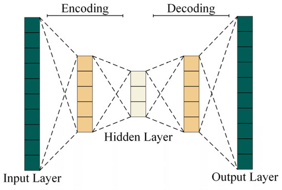
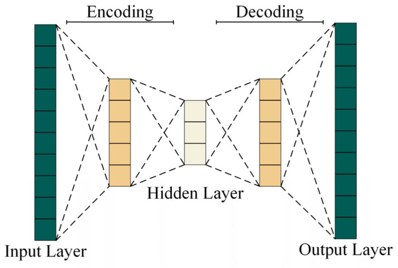
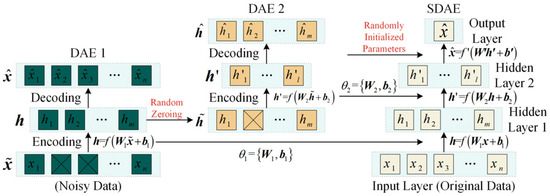
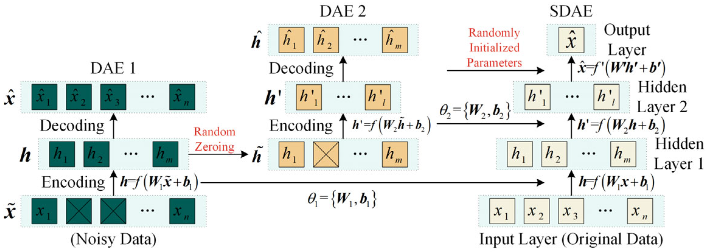
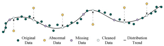
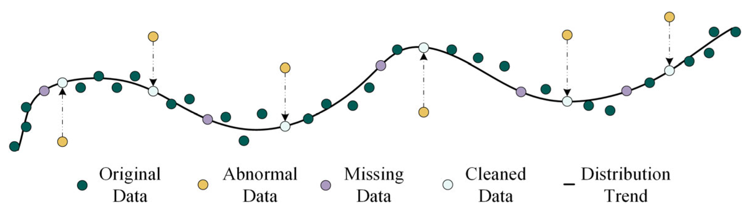
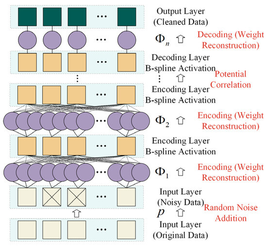
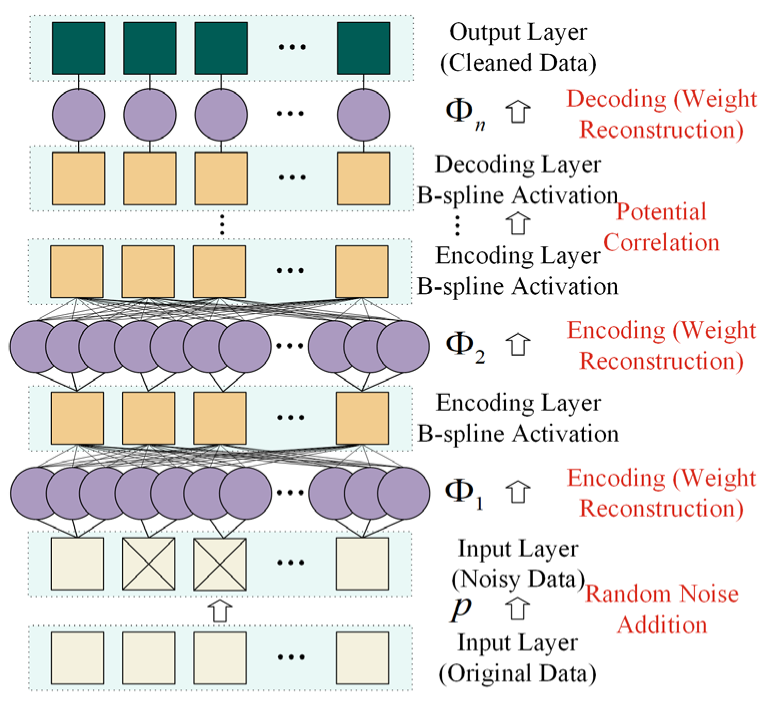
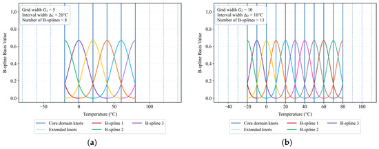
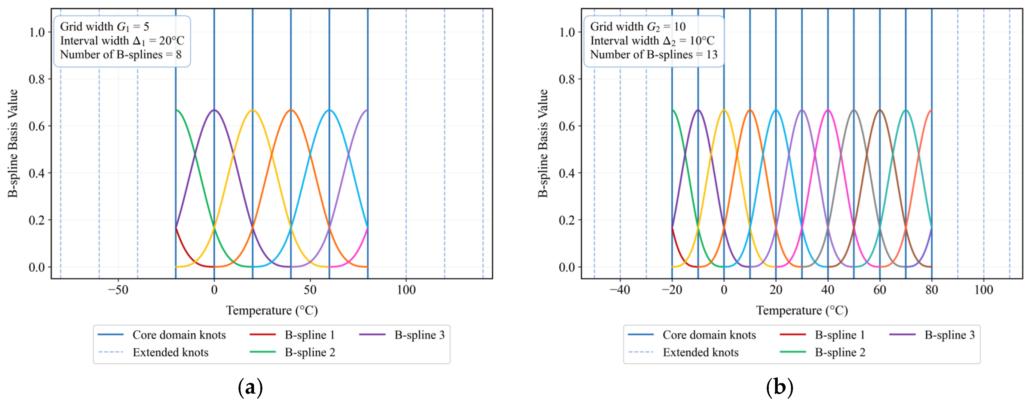
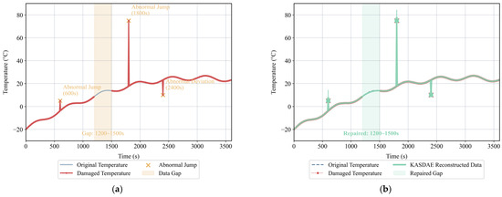
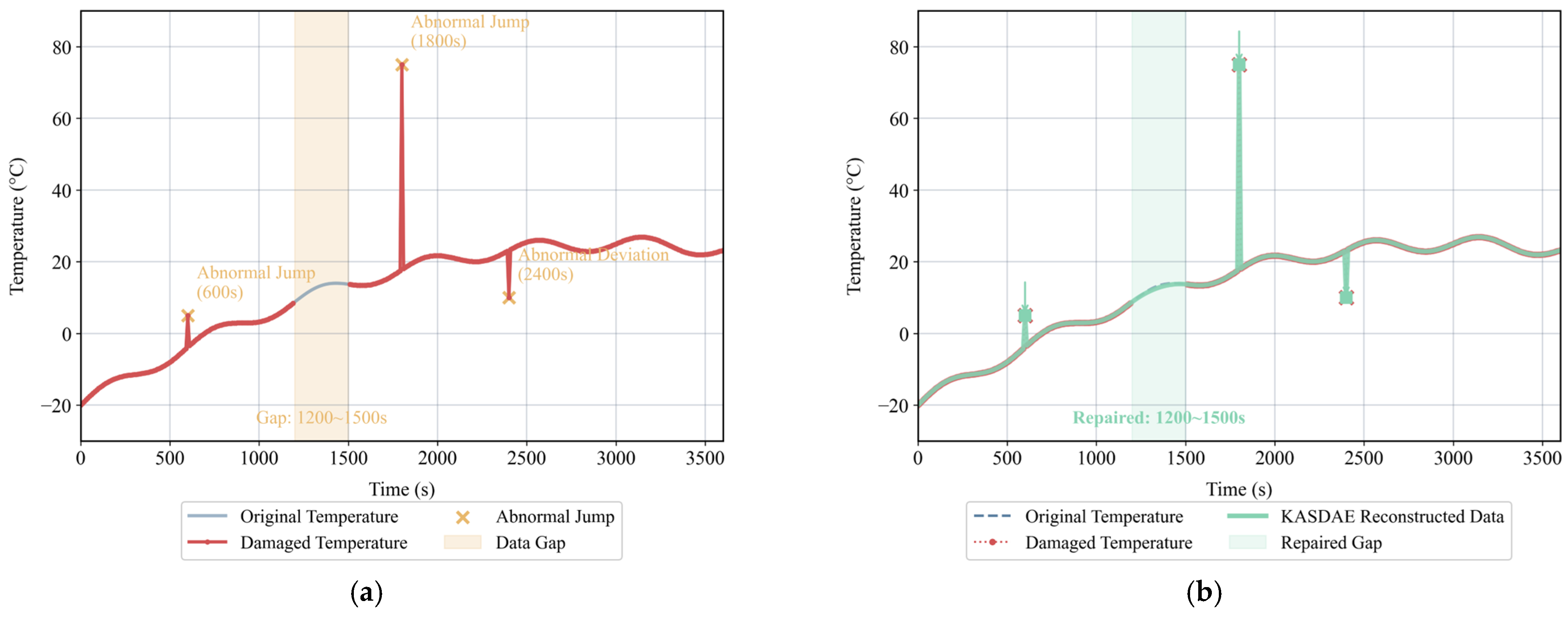
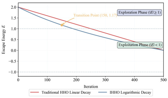
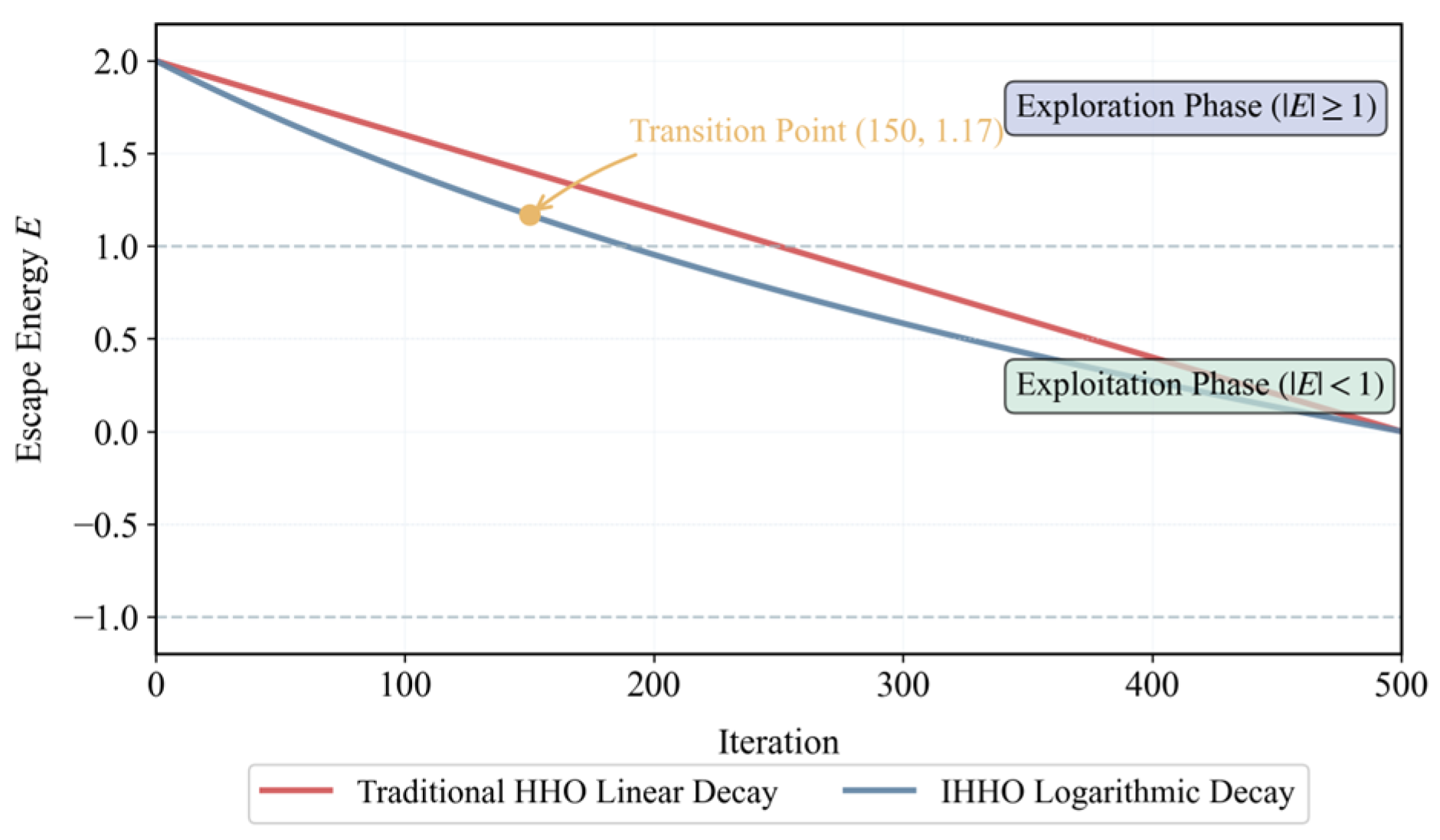
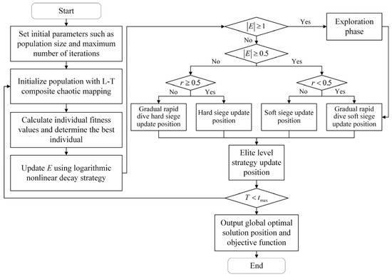
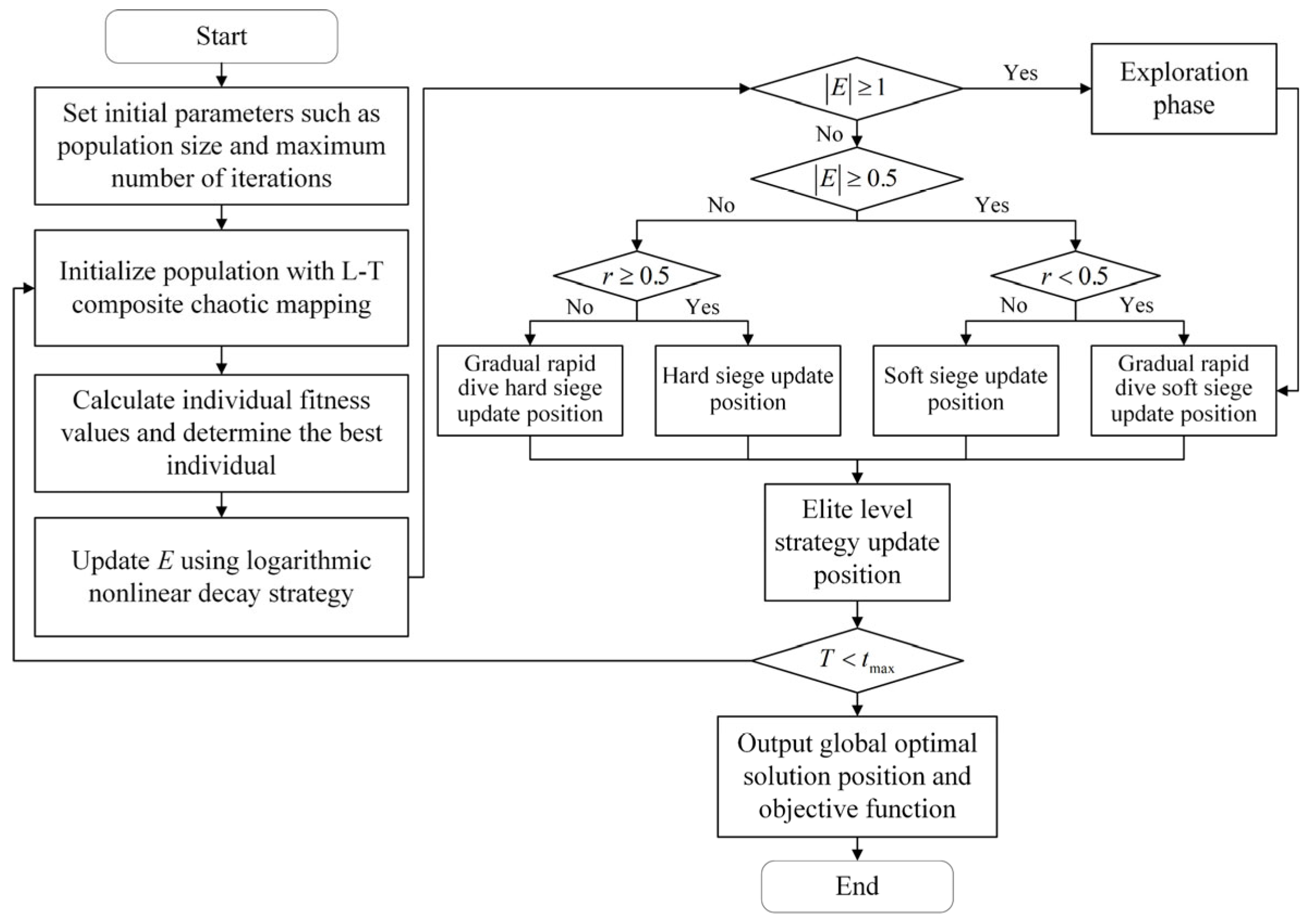
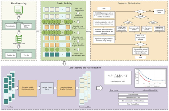
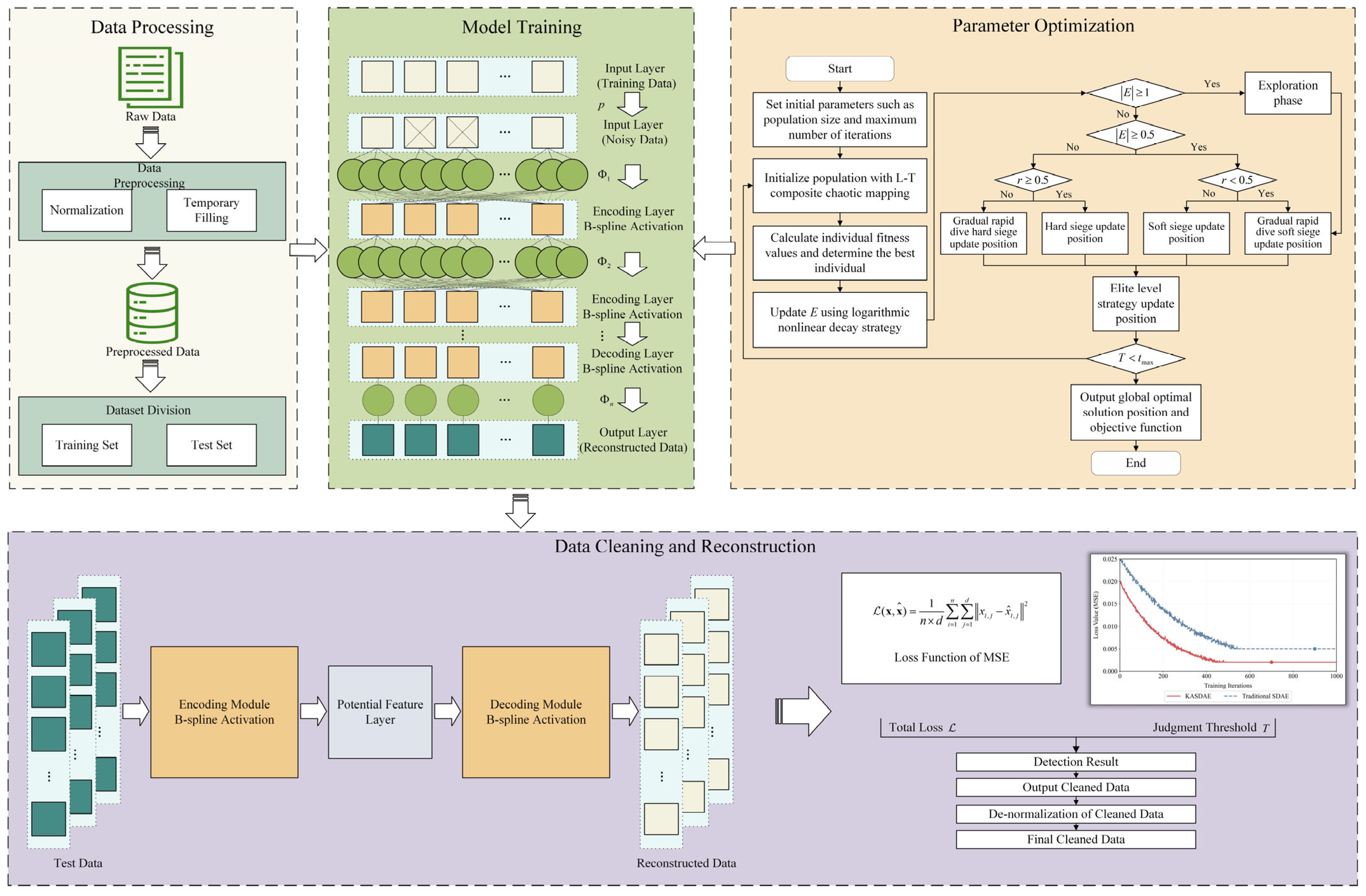
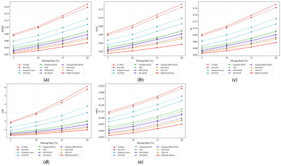
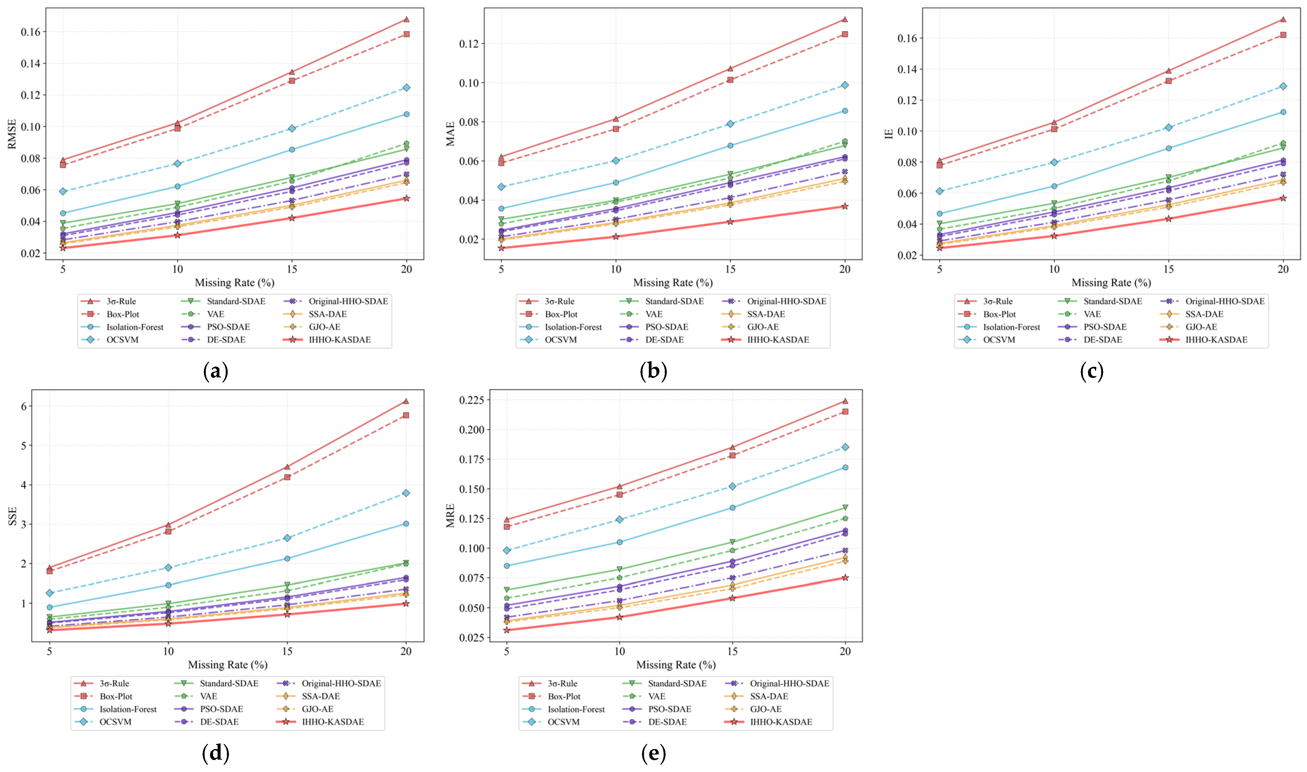
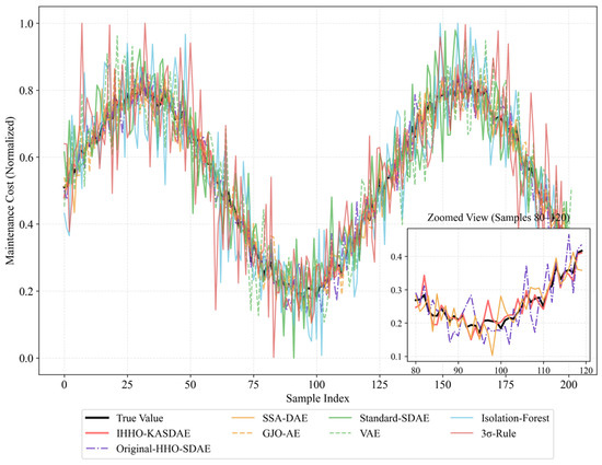
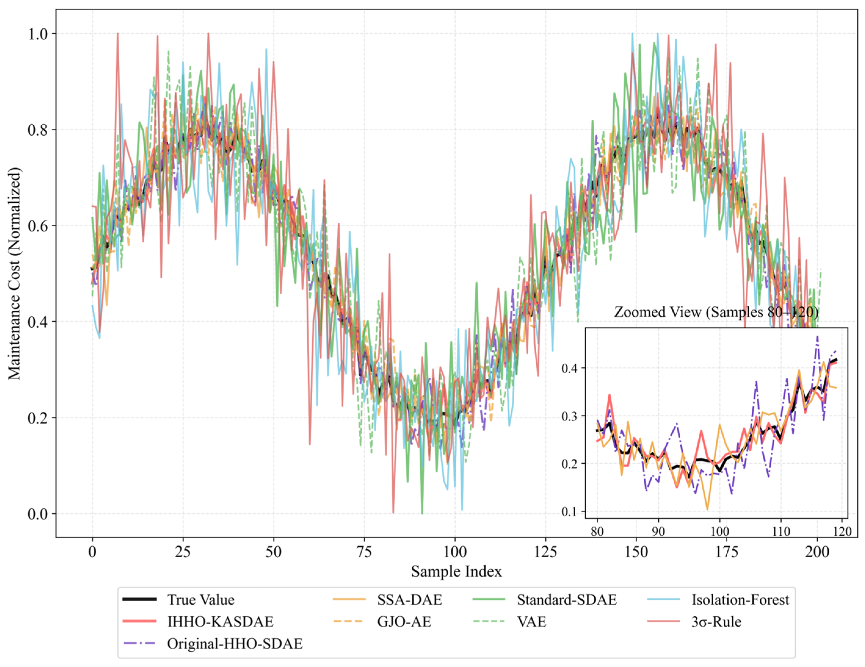
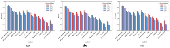
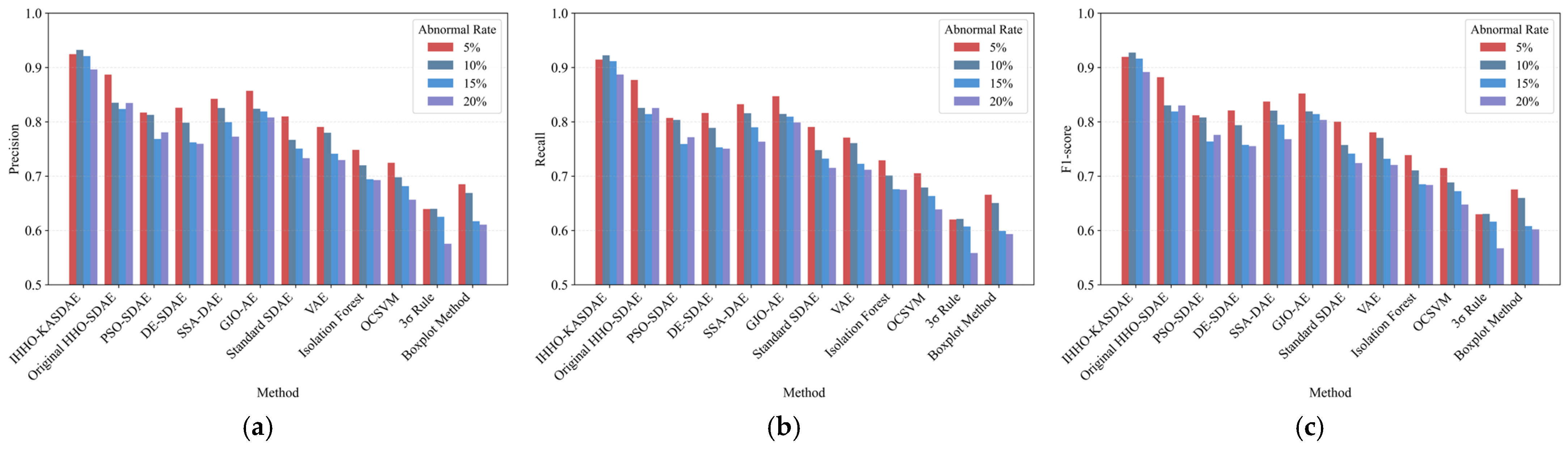
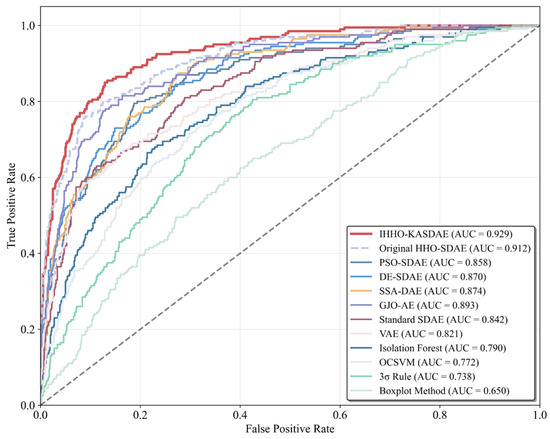
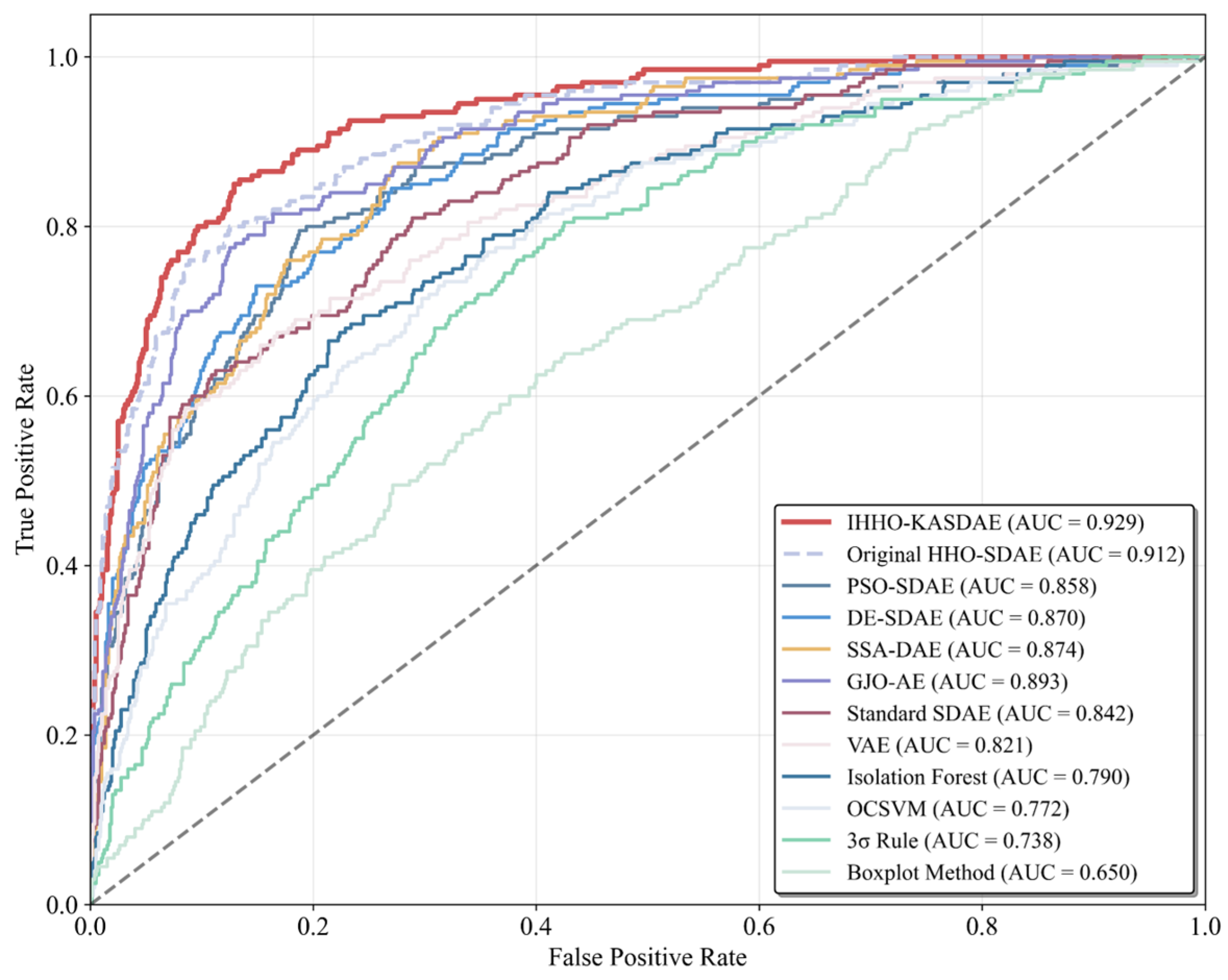
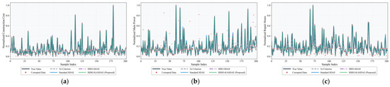
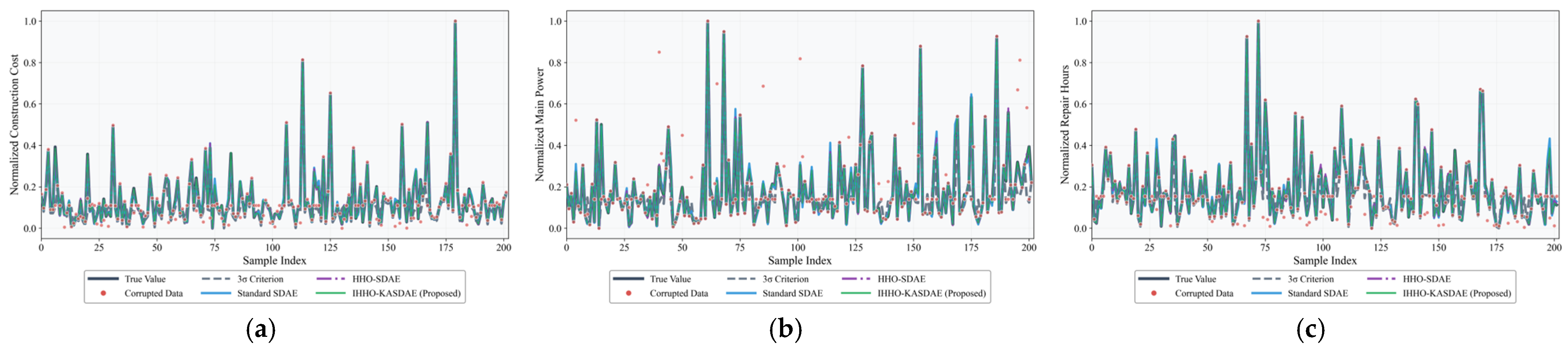
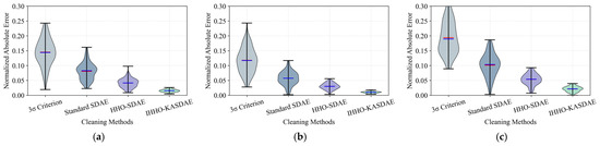
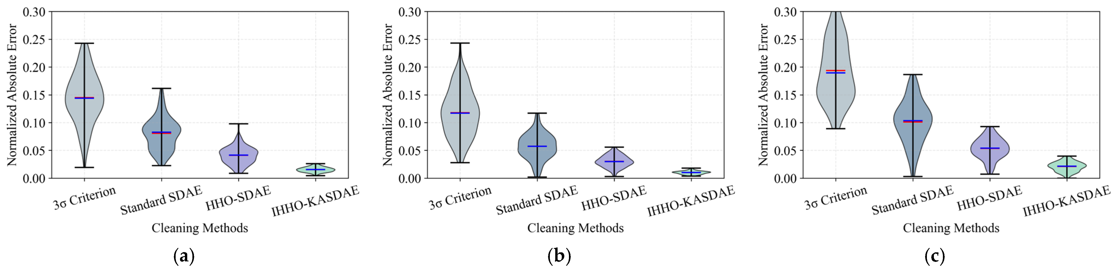
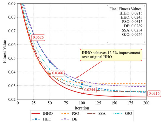
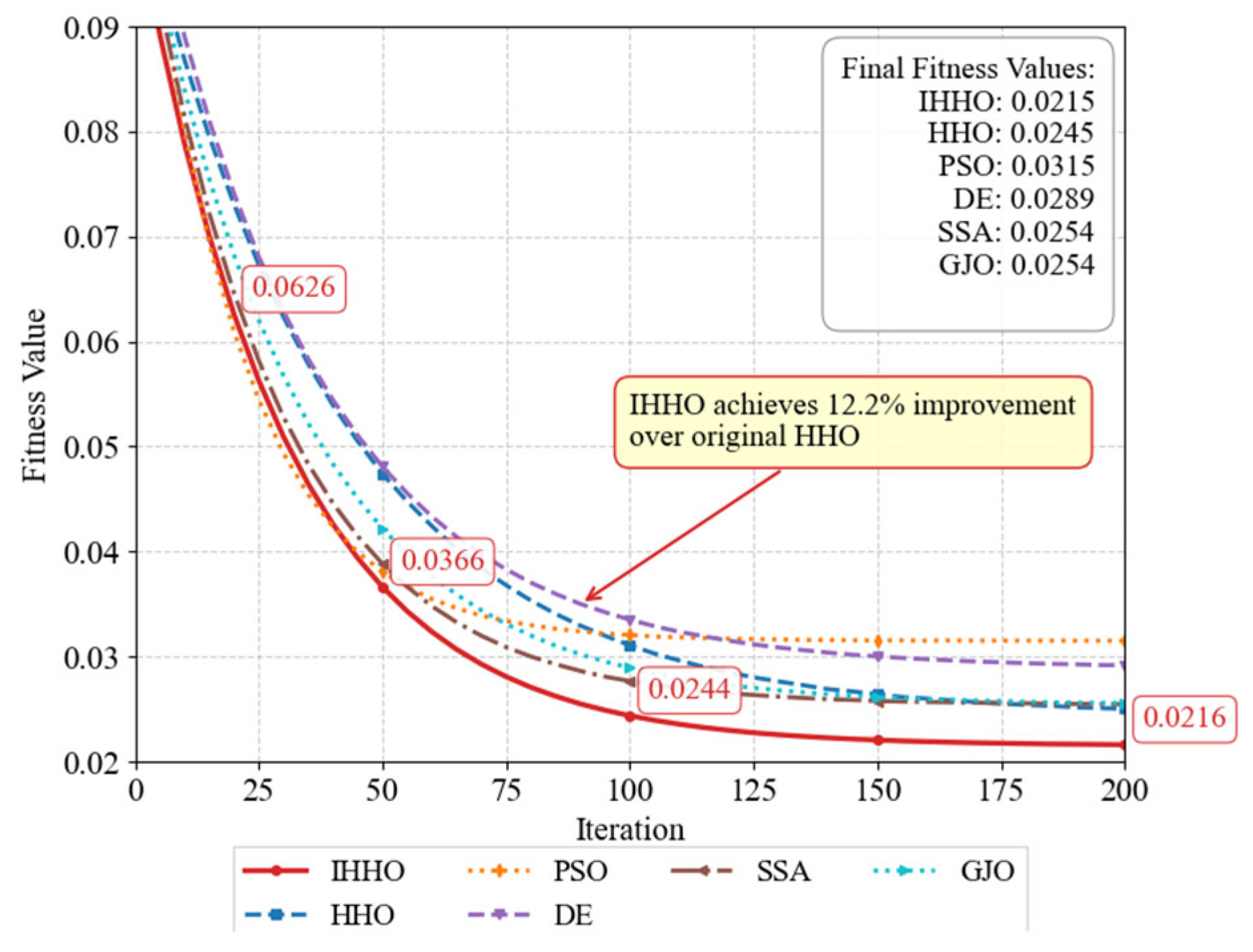
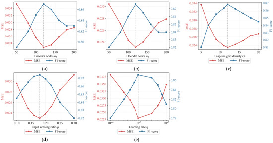
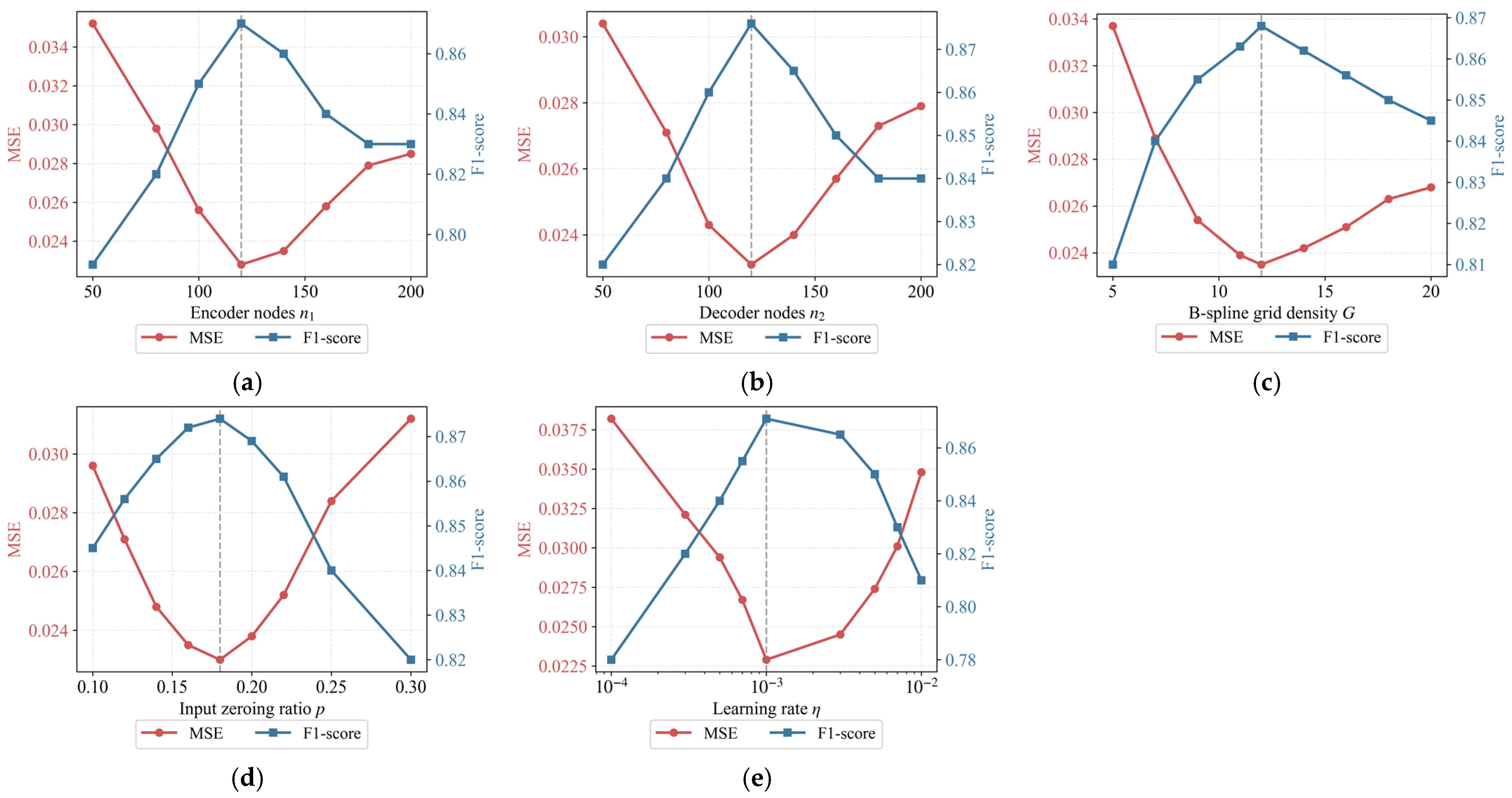
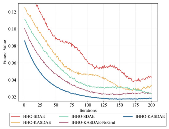
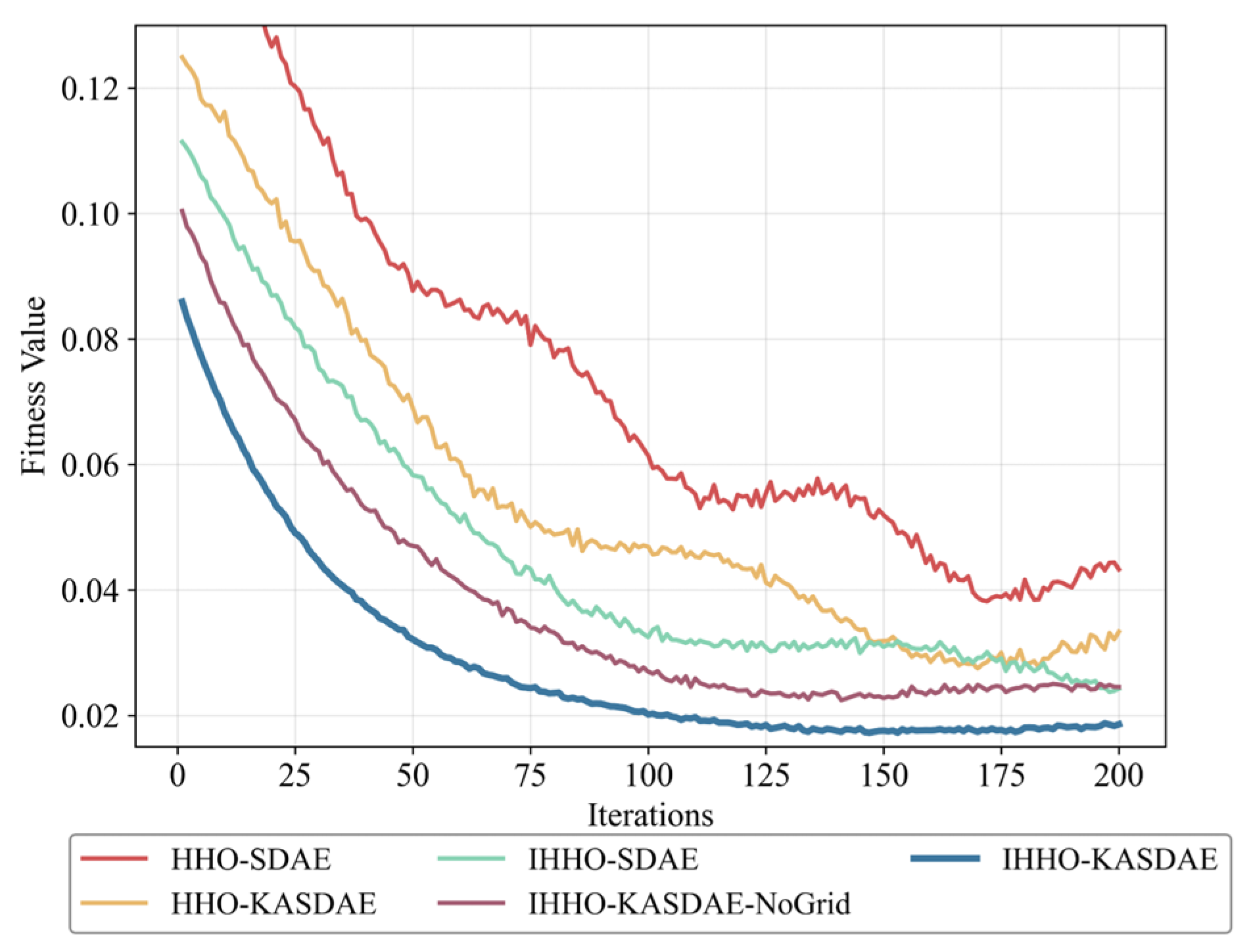
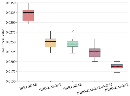
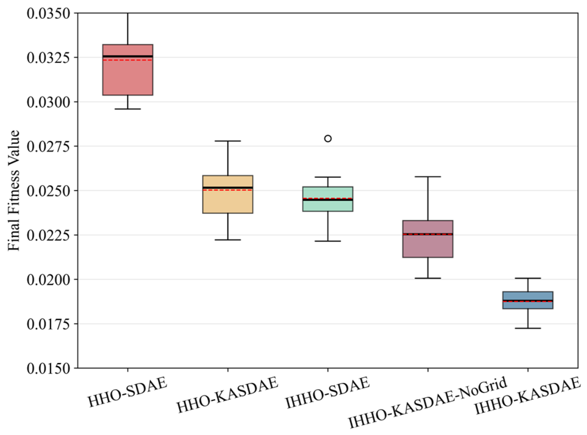

Disclaimer/Publisher’s Note: The statements, opinions and data contained in all publications are solely those of the individual author(s) and contributor(s) and not of MDPI and/or the editor(s). MDPI and/or the editor(s) disclaim responsibility for any injury to people or property resulting from any ideas, methods, instructions or products referred to in the content. |
© 2026 by the authors. Licensee MDPI, Basel, Switzerland. This article is an open access article distributed under the terms and conditions of the Creative Commons Attribution (CC BY) license.