


Abstract
Video anomaly detection is critical for information security in IoT-based intelligent surveillance, where heterogeneous sensors continuously measure the physical environment and anomalies manifest as deviations from learned normal behavior. Existing methods, however, still struggle to jointly model long-range spatio-temporal dependencies and to fuse heterogeneous multimodal measurements. Deploying such detectors on resource-constrained edge devices remains a further practical barrier. To address these challenges, we propose E-STG-DiffNet, an edge–cloud collaborative multimodal spatio-temporal graph diffusion network that formulates secure IoT surveillance as a network measurement problem. The system employs a Video Swin Transformer to extract multi-scale visual features with linear complexity. A dynamic adaptive spatio-temporal graph convolutional network (ST-GCN) with trainable node embeddings then fuses the heterogeneous sensor measurements in non-Euclidean space, and a masked latent diffusion model (MLDM) combines masked context reconstruction with stochastic denoising for anomaly scoring. A confidence-aware edge–cloud collaborative inference mechanism, supported by knowledge distillation, enables low-latency deployment. On UCSD Ped2, CUHK Avenue, and ShanghaiTech, E-STG-DiffNet reaches frame-level micro-AUC scores of 98.1%, 90.4%, and 78.3%, respectively, competitive with the strongest recent methods on these benchmarks. All results are averaged over three random seeds. Ablation studies confirm that each core component contributes to the overall performance. In the efficiency analysis, the system sustains 26.3 FPS with a mean end-to-end latency of 43 ms (99th percentile: 88 ms), while only about 10% of frames are offloaded to the cloud as compressed latents, about 0.03% of the raw-video uplink traffic. Because the public benchmarks used in our experiments do not contain real non-visual sensor streams, the temperature, vibration, and acoustic modalities are simulated following an established protocol. The reported results therefore primarily validate the video anomaly detection capability of the framework, and validation on real multimodal sensor networks is left to future work.
1. Introduction
Physical security increasingly relies on large-scale networked sensing as Internet of Things (IoT) devices become more widely deployed. Modern surveillance systems combine high-definition cameras, acoustic sensors, infrared thermal imagers, vibration monitors, and environmental probes to monitor complex scenes continuously [1,2]. Video alone does not capture every relevant signal. Cameras can show flames and smoke or record pedestrian falls, but abnormal equipment vibration, explosion sounds, and unexpected temperature increases may be easier to detect with other sensors. Security monitoring systems in smart cities, industrial facilities, and critical infrastructure therefore use video anomaly detection (VAD) together with these non-visual measurements to detect such events.
Network measurement infers the state of an environment from sensor streams that differ in modality, sampling time, and location. These streams tend to follow recurring patterns during normal operation, but attacks, accidents, and safety violations can disrupt these patterns in ways that are difficult to anticipate. A training set cannot cover every disruption that might occur. We instead train the model only on normal measurements to learn the manifold of routine behavior, following established deep anomaly detection formulations and VAD evaluation protocols [3,4]. Observations that depart from this manifold are flagged as anomalous [1,5]. Our framework uses the same procedure for anomaly scoring.
In IoT security deployments, a VAD model has to capture activity over long periods and across an entire scene without exceeding the compute budget of an edge device. ConvLSTM architectures [6] have difficulty with long sequences because their gradients may vanish, and their local receptive fields limit the scene context available to each prediction. Transformer architectures [7,8] handle long-range context better, but the cost of self-attention grows quadratically with input length. For high-resolution video, this cost makes real-time edge inference difficult. A temperature surge at one location can coincide with smoke recorded by a distant camera during the same incident. Distance-based heuristics would miss this relationship. Many methods nevertheless concatenate or stack features in Euclidean space [9,10], without modeling the irregular topology of the IoT deployment. GAN-based reconstruction models [11,12] can collapse onto a small set of modes during training. Normal patterns outside those modes are then reconstructed poorly and may be mistaken for anomalies. Edge devices may also lack the computational resources needed for real-time inference [13,14]. Sending raw measurements to the cloud avoids this local bottleneck but adds latency and increases bandwidth use. It also sends sensitive surveillance data off-site, creating additional privacy risks.
To address these challenges, we introduce E-STG-DiffNet, an edge–cloud collaborative multimodal spatio-temporal graph diffusion network for IoT video anomaly detection. Our approach exploits both the statistical regularity of normal spatio-temporal patterns and the structured deviations caused by anomalies across the sensing-to-decision pipeline. The framework focuses on combining complementary components into a unified system rather than redesigning individual building blocks, with the main contributions summarized below:
- We incorporate a hierarchical perception backbone based on the Video Swin Transformer [15] into the detection pipeline. This design captures long-range spatio-temporal dependencies with linear computational complexity and produces compact multi-scale representations of normal visual dynamics.
- We design a dynamic adaptive ST-GCN fusion module that learns semantic topology using trainable node embeddings. Learning the two embedding matrices independently yields a directed adjacency matrix that captures asymmetric cross-modal dependencies among heterogeneous IoT measurement sources in non-Euclidean space.
- We introduce a masked latent diffusion model (MLDM) that combines masked context reconstruction with stochastic denoising in a compressed latent space, together with a boundary consistency objective; this combination is designed to enlarge the reconstruction gap between normal and anomalous inputs while retaining the stable likelihood-based training of diffusion models.
- We design a confidence-aware edge–cloud collaborative inference mechanism based on knowledge distillation [16] and uncertainty-driven task offloading, in which the variance of anomaly scores across stochastic masked forward passes serves as the offloading criterion. Edge devices process easy samples locally and route only ambiguous hard samples to the cloud, reducing latency and bandwidth consumption without sacrificing accuracy.
- Experiments on UCSD Ped2, CUHK Avenue, and ShanghaiTech, each repeated with three random seeds, yield frame-level micro-AUC scores of 98.1%, 90.4%, and 78.3%, respectively, comparable to those of the strongest representative methods. Ablation and component-wise analyses quantify the contribution of each module, and the efficiency analysis reports the latency, throughput, and uplink-traffic behavior of the deployed system.
Beyond the integration itself, three design choices are central to this work. First, we formulate IoT surveillance as a measurement problem over a single dynamic heterogeneous graph in which cameras and non-visual sensors are interchangeable node types, so that cross-modal fusion is performed by learned message passing rather than by feature concatenation. Second, the MLDM couples a masked-context objective with latent-space denoising through a boundary consistency loss (Equations (12) and (13)), which is specifically designed to enlarge the reconstruction gap between normal and anomalous inputs. Third, we link the stochasticity of diffusion inference to system scheduling: the variance of anomaly scores over multiple randomly masked forward passes (Equation (19)) is used as an uncertainty signal that drives edge–cloud offloading, and a hybrid feature-plus-trajectory distillation objective (Equation (17)) transfers this behavior to the quantized edge model. These three elements, rather than any single component, constitute the primary technical contribution of the paper.
Finally, we emphasize a scope limitation of the present experiments. Audio–visual anomaly detection benchmarks with real non-visual streams do exist: XD-Violence [17], for example, provides synchronized audio for weakly supervised violence detection. The three standard benchmarks used in this study (UCSD Ped2, CUHK Avenue, and ShanghaiTech), however, contain no temperature, vibration, or acoustic measurements, and XD-Violence targets a supervised recognition setting rather than the unsupervised reconstruction-based setting studied here. The non-visual sensor streams in this work are simulated following the protocol of [18] (Section 4.3), and we additionally report a video-only variant of the framework to isolate the contribution of the simulated modalities (Section 4.4). The reported results therefore mainly establish the video anomaly detection capability of E-STG-DiffNet and the feasibility of its graph-based fusion mechanism, while the framework’s effectiveness on genuinely multimodal sensor networks remains to be verified on real deployments.
The rest of this paper is organized as follows. Section 2 reviews related work on video anomaly detection, diffusion models, spatio-temporal graph neural networks, and edge–cloud collaborative inference, linking these topics to symmetry and asymmetry in network measurement. Section 3 presents the system design, mathematical formulations, and algorithmic workflows. Section 4 describes the experimental setup, benchmark results, and component-wise analyses. Section 5 discusses the advantages and limitations of the framework and its implications for information security. Section 6 concludes the paper.
2. Related Work
2.1. Video Anomaly Detection
Video anomaly detection methods generally fall into three categories: reconstruction-based, prediction-based, and memory-augmented approaches. Reconstruction-based methods [19,20] assume that models trained only on normal data produce less accurate reconstructions for unseen anomalies than for normal inputs. Anomalous inputs therefore yield higher reconstruction errors. Hasan et al. [19] used convolutional autoencoders to learn temporal regularity, and their method remains a standard reconstruction baseline. Gong et al. [20] added a memory of normal-pattern prototypes to the autoencoder. At inference, the model retrieves prototypes from this memory for reconstruction, so anomalous inputs are less likely to be reproduced accurately.
Prediction-based methods [12,21] instead identify anomalies by comparing a predicted future frame with the frame actually observed. Liu et al. [12] introduced a widely used baseline of this type, in which a U-Net is trained adversarially to predict future frames. Park et al. [22] combined reconstruction and prediction objectives in a memory-guided architecture.
Transformers and hybrid generative models have also been used for VAD. Ristea et al. [7] used self-distilled masked autoencoders to trade off accuracy against inference speed on server-grade GPUs. Hirschorn and Avidan [8] modeled normal human pose sequences with spatio-temporal graph normalizing flows and reported competitive results on ShanghaiTech. Liu et al. [23] combined memory-augmented optical flow reconstruction with flow-guided frame prediction in HF2-VAD and reported high frame-level AUC on standard benchmarks. Although these methods improve long-range and generative modeling, they do not address heterogeneous multimodal inputs or the resource limits of IoT edge deployments.
2.2. Diffusion Models for Anomaly Detection
Denoising diffusion probabilistic models (DDPMs) [24,25] learn to reverse a forward diffusion process rather than relying on adversarial optimization. Compared with GANs, they generally train more stably and can produce higher-quality samples with better mode coverage for complex distributions.
Diffusion-based anomaly detection has been studied in both medical imaging and video. Wolleb et al. [26] localized pathological regions by comparing an abnormal medical image with its diffusion-reconstructed healthy counterpart. For VAD, Zhou et al. [27] guided patch diffusion with motion and appearance in MA-PDM. Their model captures localized dynamics and achieves high frame-level accuracy. Zhang et al. [28] proposed DiffVAD, which performs unsupervised VAD through diffusion-based latent pattern learning.
Diffusion models have also been applied to input types beyond unimodal video. For example, Hu et al. [29] developed AnomalyXFusion, which synthesizes anomalies by combining image, text, and mask representations. Flaborea et al. [30] used motion-conditioned diffusion for skeleton-based VAD and reported strong results. These studies suggest that diffusion models can provide broader mode coverage and more reliable anomaly scoring than adversarial baselines. We therefore use diffusion in the proposed architecture.
2.3. Spatio-Temporal Graph Neural Networks
Spatio-temporal graph convolutional networks (ST-GCN) were originally proposed by Yan et al. [9] for skeleton-based action recognition. Their key idea is to model the human skeleton as a graph and apply graph convolutions along both the spatial and temporal dimensions. Subsequent works have introduced adaptive graph learning mechanisms to overcome the limitations of predefined graph structures. Li et al. [10] proposed actional–structural graph convolutional networks that learn both structural and actional links between joints. Shi et al. [31] introduced a two-stream adaptive graph convolutional network that learns the graph topology directly from data. In the context of anomaly detection, Luo et al. [32] applied spatial–temporal graph convolutional encoders to extract pose sequences for anomaly detection, whereas Markovitz et al. [33] used graph-embedded pose clustering to detect anomalous human activities. Recent research has also extended graph neural networks to heterogeneous multimodal data fusion scenarios. Deng and Hooi [34] proposed a GNN-based approach for anomaly detection in multivariate time series, showing that graph structures are effective at capturing inter-sensor dependencies. These advances motivate the use of adaptive ST-GCN for fusing heterogeneous IoT sensor data in this work.
2.4. Edge–Cloud Collaborative Inference
Large detection models are often too expensive to run on IoT edge devices. Edge–cloud inference can move computation between these devices and cloud servers to balance processing latency and inference accuracy [13,35]. Knowledge distillation (KD) [16] provides a compact model for local execution by training a lightweight student network to mimic a larger teacher.
Yang et al. [18] used lightweight statistical filters at the edge and deep models in the cloud for anomaly detection in industrial sensor networks. Ferrari et al. [35] compared cloud-only and edge–cloud configurations and reported lower latency and bandwidth use for hybrid execution. Abbasi et al. [36] studied deep-learning-based anomaly detection in IoT edge computing with instance-level horizontal reduction. In our diffusion-based detection pipeline, we use reconstruction uncertainty to make a per-input deployment choice: predictable inputs are processed locally, whereas ambiguous or complex ones are sent to the cloud.
2.5. Symmetry and Asymmetry in Network Measurement and Anomaly Detection
Symmetry and asymmetry provide a useful perspective on anomaly detection and network measurement. In standard formulations, normal data are assumed to lie on a low-dimensional manifold or follow a distribution with compact support [19,20]. Models fitted to normal data can therefore reliably reconstruct, predict, or generate typical observations. Anomalies depart from these regularities because they occur infrequently and differ structurally from baseline behavior, leading to higher reconstruction errors or lower likelihood scores under the trained model.
Network operators face the same difficulty: normal traffic is easier to characterize than every possible fault or attack. Traffic matrices, telemetry streams, and sensor topologies have recurring spatial and temporal patterns, and departures from these patterns may signal intrusions, system faults, or attacks [18,34]. In intrusion detection and encrypted traffic analysis, benign flows often have regular packet sizes and stable periodicity. Scanning, flooding, and protocol anomalies alter these profiles. The deployment architecture is also asymmetric: edge units have limited resources, while cloud servers operate under different latency and accuracy constraints [13,35]. Our graph diffusion process learns the normal structure and uses deviations from it to detect anomalous events.
3. System Design
E-STG-DiffNet is organized into four layers: perception, fusion, generation, and collaborative inference. The following sections describe each layer in turn.
3.1. Overall Architecture
We represent the IoT surveillance network as a dynamic heterogeneous graph . The graph has camera nodes and non-visual sensor nodes. Together they form , where . Edges in represent spatio-temporal dependencies between nodes, and their weights form the adjacency matrix .
The edge tier and the cloud share computation. The edge tier acquires and preprocesses local data, then uses a lightweight student model for real-time inference on high-confidence samples. Ambiguous samples are sent to the cloud, where the full teacher model processes them. The cloud also handles periodic retraining and updates to the global topology. Figure 1 shows how these components interact.
Figure 1.
Overall architecture of E-STG-DiffNet. On the edge device, the student model extracts multimodal features, performs ST-GCN fusion, and uses masked diffusion for reconstruction. When confidence is low, the cloud teacher performs full inference and uses a vision–language model (VLM) to interpret the event semantically. The cloud periodically sends distillation updates back to the edge.
3.2. Perception Layer: Video Swin Transformer
We use the Video Swin Transformer [15] as the visual backbone instead of ConvLSTM. It computes self-attention in local 3D windows and shifts the window partitions between layers to connect them. This gives the model access to the global scene context without applying attention over the entire clip.
3.2.1. 3D Patch Partition and Linear Embedding
We divide the input clip into non-overlapping 3D patches of size , such as . Each patch is flattened and passed through a linear embedding layer to produce a C-dimensional token:
where is the projection matrix. The result is a 3D grid of tokens, each describing a local spatio-temporal region of the clip.
3.2.2. 3D Shifted Window Self-Attention
Attention is restricted to non-overlapping 3D windows of size , which limits computation and adds a locality inductive bias. Regular window attention (W-MSA) and shifted window attention (SW-MSA) alternate from one layer to the next so that information can pass between windows. The corresponding updates for layers l and are
Here, is layer normalization, and consists of two linear transformations with a GELU activation.
3.2.3. 3D Relative Position Encoding
We include relative spatial and temporal positions by adding a 3D position bias to the attention matrix:
Since attention is computed within windows, its cost scales as with the number of tokens rather than quadratically as in standard Transformers. Shifted windows still let information pass between distant regions and across time.
3.3. Fusion Layer: Dynamic Adaptive ST-GCN
A spatio-temporal graph convolutional network (ST-GCN) [9] fuses the Video Swin features with non-visual sensor measurements on an adaptive graph. Learning this graph allows distant devices to be linked when their measurements refer to the same event. A temperature sensor and a surveillance camera, for example, may both provide evidence of a fire from different locations.
3.3.1. Adaptive Graph Structure Learning
A fixed adjacency matrix based on sensor locations cannot represent relationships that change with the event being observed. E-STG-DiffNet instead learns end-to-end. Two independently parameterized node embedding matrices, , define the topology as follows:
The learned entries can link a change in thermal readings with a simultaneous visual anomaly without using device coordinates. ReLU sets negative affinity scores to zero. Softmax then normalizes each row into a distribution over candidate neighbors.
The two embedding matrices are learned separately, so need not be symmetric. The learned graph is therefore directed: is the attention weight from node i to node j and can differ from the reverse weight. This allows unequal influence between modalities. During an incident, for example, camera features may strongly shape the representation of a nearby acoustic sensor, while the acoustic signal contributes little to the camera representation. A static undirected proximity graph cannot encode this distinction.
3.3.2. Sensor Feature Encoding
Each non-visual sensor i has a raw time series . A 1D convolutional neural network (1D-CNN) converts it to a temporal feature sequence with the common dimension D:
The Video Swin features for camera nodes are mapped to the same dimension with a linear layer: .
3.3.3. Spatio-Temporal Graph Convolution
We concatenate the projected visual features and sensor features to form . The ST-GCN then applies spatial aggregation followed by temporal modeling.
Spatial Aggregation
Graph convolution first exchanges information between modalities:
Here, is a learnable parameter matrix and is the activation. Adding creates self-loops, so each node keeps its own features while receiving messages from other nodes.
Temporal Evolution
The gated TCN then models how these node features change over time:
Here, * denotes temporal convolution, and are temporal convolution kernels, and ⊙ is the Hadamard product. The gate controls which temporal information is retained, allowing the model to suppress high-frequency noise without discarding task-relevant dynamics. The output is , a latent summary of the spatio-temporal interactions across modalities.
3.4. Generation Layer: Masked Latent Diffusion Model
Normal behavior is modeled with a masked latent diffusion model (MLDM). The diffusion process provides stochastic perturbations for anomaly scoring, while spatial masks require the model to reconstruct missing content from its surrounding context.
3.4.1. Latent Space Mapping
Iterative denoising in the original feature space would be computationally expensive. We therefore use a pretrained variational autoencoder (VAE) to encode in a lower-dimensional latent space:
The latent representation retains the spatial structure and temporal cues needed for reconstruction but makes repeated denoising substantially cheaper.
3.4.2. Forward Diffusion Process
A Markov chain gradually corrupts each normal latent vector with Gaussian noise:
where specifies the noise variance at step t. Defining allows to be sampled directly without iterating through all preceding steps:
We adopt the cosine variance schedule of Nichol and Dhariwal [37] rather than the linear schedule used in standard DDPMs, since the latter can destroy too much structure in the early steps. The same isotropic Gaussian perturbations are applied to every normal training latent. Reverse estimation therefore learns to recover samples from the normal data distribution; inputs inconsistent with that distribution should leave larger reconstruction residuals.
3.4.3. Masking Strategy and Denoising Training
Random masks discourage the denoiser from copying its input. Following the masking principle in masked autoencoders [38], a binary mask hides a fixed proportion of latent tokens, such as 75%. A U-Net denoising network [39] predicts the injected noise from the noisy state and the unmasked context.
Training uses the diffusion reconstruction error together with a penalty on discontinuities at mask boundaries:
where controls the contribution of the boundary penalty. For the boundary set between masked and observed elements, this term is
where is the reconstructed representation at location i. The penalty discourages abrupt spatial or temporal changes where reconstructed content meets observed content.
3.4.4. Anomaly Scoring Mechanism
At inference time, the VAE encoder maps an input sample to . Noise is added up to an intermediate step t, and a spatial mask is applied before the reverse process estimates the clean representation . Masked regions are reconstructed according to the normal patterns observed during training. The discrepancy between the input and its reconstruction gives the anomaly score
Large residuals identify candidate anomalous regions in the latent representation. At a fixed detection rate, Section 4.6 shows that MLDM produces fewer false alarms on normal frames than the AE, VAE, and GAN baselines. Repeating the procedure K times with independently sampled masks also yields an uncertainty estimate from the score variance (Equation (19)).
3.5. Collaborative Layer: Edge–Cloud Inference
A full teacher model in the cloud supervises a lightweight student model deployed on edge nodes. During inference, the student handles samples with consistent predictions and sends uncertain cases to the cloud. This division of work limits latency and uplink traffic, and avoids routinely transmitting raw surveillance video.
3.5.1. Cross-Modal Knowledge Distillation
The student is obtained from the teacher through structured pruning and INT8 quantization. Compression can degrade detection performance, so training matches both intermediate features and denoising outputs.
Feature Distillation
A projection layer maps student features to the teacher’s feature space before their discrepancy is measured:
where and extract intermediate features from the teacher and student, respectively, and is a learnable projection that matches their channel dimensions.
Response Distillation
The student is also trained to reproduce the teacher’s noise predictions throughout the reverse denoising trajectory:
where and are the noise estimates produced by the teacher and student denoising networks. The two losses are weighted as
where determines the relative weight of feature matching and noise prediction.
3.5.2. Confidence-Aware Task Offloading
The edge device uses the variability of the student’s predictions to decide whether cloud verification is necessary. Samples with low uncertainty are returned locally, while the remaining samples are offloaded:
where is the offloading threshold. The uncertainty is the variance of anomaly scores obtained from K forward passes with independently sampled masks:
where is the reconstruction from the k-th pass. If small changes to the mask produce substantially different scores, the edge prediction is treated as unreliable and the sample is sent to the teacher.
Most normal instances can therefore be handled without a cloud round trip, while bandwidth is spent on cases for which local inference is less stable. Offloaded requests contain compressed latent vectors rather than raw video. Section 4.9 reports that this procedure reduces uploaded frames by approximately 90% and uplink traffic to about 0.03% of the volume required for raw-video streaming.
3.5.3. VLM-Based Semantic Enhancement
Confirmed alarms can also include a short textual description. The cloud passes four uniformly sampled keyframes to LLaVA-1.5-7B [40], an off-the-shelf vision–language model (VLM) used without task-specific fine-tuning, together with the prompt “Describe the unusual event in these surveillance frames in one sentence.” Example outputs include “a person riding a bicycle in a pedestrian area” for UCSD Ped2 and “a person throwing an object” for CUHK Avenue. Reviewers see these descriptions alongside the numerical anomaly scores. Human ratings of the generated captions are reported in Section 4.13.
3.6. Algorithm
The complete inference and collaborative workflow of E-STG-DiffNet is summarized in Algorithm 1.
| Algorithm 1 E-STG-DiffNet Edge–Cloud Collaborative Anomaly Detection |
|
4. Experiments
This section evaluates E-STG-DiffNet on three benchmark datasets through comparisons with state-of-the-art methods, ablation studies, and detailed analyses of individual components.
4.1. Datasets
We use three widely used video anomaly detection benchmarks. UCSD Ped2 [41] contains 16 training and 12 test videos of pedestrian walkways captured at a resolution of pixels; anomalies include bicycles, vehicles, and skateboards appearing in pedestrian-only areas, and all frames are resized to for processing. CUHK Avenue [42] comprises 16 training and 21 test clips of a campus avenue, with anomalies such as running, throwing objects, and loitering; compared with UCSD Ped2, it contains more diverse anomaly types and more complex backgrounds. ShanghaiTech [43] is the largest and most challenging of the three, with 330 training and 107 test videos from 13 different scenes and 130 anomalous events across various categories, including chasing, brawling, and sudden motions; its multi-scene nature is particularly challenging for methods that rely on scene-specific modeling.
4.2. Evaluation Metrics
We use the frame-level Area Under the Receiver Operating Characteristic Curve (AUC) as the primary metric, following standard practice in video anomaly detection [1]. AUC measures how well the model distinguishes normal from anomalous frames across all decision thresholds, and higher values indicate better detection performance. We also report the Equal Error Rate (EER) as a complementary metric, with lower values indicating better accuracy.
4.3. Implementation Details
Experiments are run on a server with four NVIDIA A100 (80 GB) GPUs (NVIDIA Corporation, Santa Clara, CA, USA) and Intel Xeon Platinum 8380 CPUs (Intel Corporation, Santa Clara, CA, USA). Edge measurements are obtained on an NVIDIA Jetson AGX Orin (64 GB; NVIDIA Corporation, Santa Clara, CA, USA). The visual backbone is Video Swin-T pretrained on Kinetics-400 [44]. It processes 16-frame clips () at resolution with a patch size of and outputs dimensional features. The ST-GCN contains nodes and uses dimensional embeddings. Each of its four layers has spatial and temporal kernel sizes of 3, followed by batch normalization and dropout (). For MLDM, the VAE produces a 256-dimensional latent representation. The U-Net denoiser has channel multipliers and applies self-attention at and resolutions. Diffusion uses steps with a cosine variance schedule, and 75% of the latent tokens are masked.
The network is trained for 200 epochs using Adam, a learning rate of , and a batch size of 16. We set . A 10-epoch warm-up precedes cosine annealing of the learning rate. The student combines Swin-T/2, half the teacher’s channel capacity, and INT8 quantization. Distillation continues for 50 epochs with . All benchmarks use a graph with nodes, comprising camera-region nodes on an grid and sensor nodes for temperature, vibration, and acoustic measurements. The 13 scenes in ShanghaiTech share this graph. Region nodes are assigned normalized grid coordinates, and a 13-dimensional one-hot scene vector is appended to each node representation. The adaptive adjacency is thus learned jointly across scenes without discarding scene identity. At inference, the latent variables are noised to and reconstructed with deterministic DDIM sampling [45], using 20 steps for the edge student and 50 for the cloud teacher. Uncertainty in Equation (19) is estimated from passes with independent masks. These passes are batched on the edge GPU and included in the measured 38 ms latency reported in Section 4.9. The threshold , computed from normalized score variance, is calibrated so that approximately 10% of frames are sent to the cloud.
Each dataset contributes 20% of its training videos to a validation split, leaving the test sets untouched during model selection. The masking ratio, sampling steps, and thresholds and are chosen on this split, as are the remaining hyperparameters. Section 4.7 and Section 4.12 likewise report validation results in their parameter analyses. Test data are used only for the final evaluation. Every experiment is repeated with seeds . AUC values are averaged over these seeds unless stated otherwise; Table 1 also gives the standard deviations. The ablation and backbone analyses also report standard deviations, while later tables omit them because the standard deviations are below 0.3 AUC points.
Table 1.
Frame-level micro-AUC (%) comparison on three benchmark datasets, following standard evaluation protocols [1]. Baseline results are taken directly from the original papers, in which models are trained only on normal data; “–” indicates unreported metrics. STG-NF evaluates estimated human poses rather than raw RGB frames and is included for reference. E-STG-DiffNet results are reported as mean ± standard deviation across three random seeds. EER (%, lower is better) is the three-dataset average and is reported only for our method because prior work reports this metric inconsistently. Bold and underlined numbers indicate the best and second-best results, respectively. Ties in average AUC are resolved using unrounded values.
Since the visual benchmarks provide no sensor measurements, we generate synthetic streams using the protocol of Yang et al. [18]. The generator models baseline dynamics, transient events, and cross-modal coupling. Temperature, vibration, and acoustic channels follow first-order autoregressive processes around nominal values of 25 °C, 0.2 g, and 45 dB, with noise standard deviations of 0.5 °C, 0.05 g, and 2 dB, respectively. Transient spikes have amplitudes between and , durations of 0.5–2 s, and onset delays of 0–0.5 s, and occur at a rate of 0.02 per video-second. Spike generation follows the same procedure in the training and test splits and is independent of the ground-truth anomaly labels, preventing direct label leakage. Half of the spikes depend on frame-level optical-flow magnitude to introduce a physical association with the video without using annotation-based supervision. These streams provide a controlled setting for testing multimodal fusion; they do not replace evaluation with physical sensors. Table 1 therefore also includes a video-only E-STG-DiffNet baseline, which separates the contribution of the simulated streams from that of the rest of the model. Section 4.4 and Section 5.3 discuss this comparison further.
4.4. Comparison with State-of-the-Art Methods
We compare E-STG-DiffNet with representative methods from several paradigms: reconstruction-based (ConvLSTM-AE [6], MemAE [20]), prediction-based (MNAD [22]), hybrid flow reconstruction and prediction (HF2-VAD [23]), masked-autoencoder-based (Ristea et al. [7]), pose-based normalizing flows (STG-NF [8]), and diffusion-based (DiffVAD [28], MA-PDM [27]) methods. Table 1 presents the quantitative comparison results. All reported AUC values are frame-level micro AUC, computed by pooling the test frames of all videos before evaluating the ROC curve, which is the standard protocol of the benchmarks [1]. Baseline results are quoted from the original papers, and all compared methods follow the same training regime, in which only the normal training videos of each dataset are used. The seed-to-seed standard deviation of E-STG-DiffNet does not exceed 0.3 AUC points on any of the three datasets.
E-STG-DiffNet achieves the highest average AUC across the three datasets (88.9%, statistically tied with HF2-VAD when rounded to one decimal place) and ranks among the top three RGB-based methods on each individual benchmark. On UCSD Ped2, E-STG-DiffNet attains 98.1%, second only to HF2-VAD (99.3%), which benefits from explicit optical-flow reconstruction at a higher computational cost. On CUHK Avenue, Ristea et al. [7] (91.3%) and HF2-VAD (91.1%) lead, with E-STG-DiffNet close behind at 90.4%; we note that the method of Ristea et al. is highly efficient on server-grade GPUs but does not address multimodal fusion or edge deployment. On ShanghaiTech, STG-NF reports a higher AUC (85.9%) but operates on extracted human pose sequences rather than RGB appearance, requires an external pose estimator and tracker, and does not report results on UCSD Ped2 or CUHK Avenue; among RGB-based methods, Ristea et al. (79.1%) lead and E-STG-DiffNet ranks second at 78.3%. Compared with the diffusion-based baselines DiffVAD and MA-PDM, which are the closest in spirit to our approach, E-STG-DiffNet improves the average AUC by 3.2 and 1.5 percentage points, respectively, while additionally supporting edge deployment.
To isolate the contribution of the simulated sensor modalities, Table 1 also reports a video-only variant of E-STG-DiffNet in which the sensor nodes are removed and the ST-GCN operates over the 64 camera-region nodes only. This variant attains 97.6%, 89.6%, and 77.4% (average 88.2%), showing that most of the detection performance stems from the core video pipeline; the simulated sensor fusion contributes a further 0.7 AUC points on average, a figure that should be interpreted as an upper bound obtained under label-independent simulation (Section 4.3) rather than as evidence of real multimodal gains. In terms of EER, E-STG-DiffNet attains 5.4%, 17.2%, and 28.6% on the three datasets (17.1% on average), consistent with its AUC ranking. Figure 2 visualizes the AUC performance across all datasets.
Figure 2.
Frame-level micro-AUC comparison on (a) UCSD Ped2, (b) CUHK Avenue, and (c) ShanghaiTech datasets. Gray bars denote previously published baselines, while the dark-red and bright-red bars denote E-STG-DiffNet (video-only) and E-STG-DiffNet (full), respectively. STG-NF is hatched and marked with an asterisk because it uses estimated human poses rather than raw RGB frames and is included for reference. E-STG-DiffNet achieves the highest average AUC across all three benchmarks and ranks among the top three RGB-based methods on each dataset.
Figure 3 presents the ROC curves of E-STG-DiffNet on all three datasets, illustrating the trade-off between the true-positive rate and the false-positive rate at various threshold settings.
Figure 3.
ROC curves of E-STG-DiffNet on the three benchmark datasets. The curves rise steeply in the low false-positive-rate region, the operating regime most relevant to surveillance applications.
4.5. Ablation Study
To measure the contribution of each core component, we conduct ablation studies on the UCSD Ped2 dataset. We progressively add components to a ResNet+AutoEncoder baseline and record the improvement in AUC. Table 2 and Figure 4 present the results.
Table 2.
Ablation study results on UCSD Ped2 (frame-level micro-AUC, %, mean ± std over three seeds). Each row adds one component to the previous configuration. All rows are evaluated at the default 20-step DDIM inference configuration; at the 50-step cloud configuration, the full model of row 4 attains 98.3%, which constitutes the accuracy upper bound of the system. The ✓ symbol indicates that the corresponding component is enabled, and the bold value indicates the best result.
Figure 4.
Ablation study: Progressive contribution of each component to the overall AUC on UCSD Ped2. Each bar shows the cumulative AUC, with the increment from the previous configuration annotated.
We analyze the contribution of each module in turn. Replacing ResNet with the Video Swin Transformer yields a +4.3% improvement, showing that long-range spatio-temporal modeling matters for capturing global scene context. Adding ST-GCN fusion gives an additional +2.8% gain; we note that this gain is obtained with the simulated sensor streams of Section 4.3, since the RGB-only variant has no sensor nodes to fuse, and it should therefore be interpreted as evidence that the graph fusion mechanism functions as intended under simulation rather than as a quantification of real multimodal benefits. Replacing the standard autoencoder with the masked diffusion model contributes +3.3%, indicating that diffusion models are better suited to reconstruction-based anomaly detection. Finally, the edge–cloud collaborative mechanism adds +0.5% and brings the system to 98.1%, within 0.2 points of the cloud-only teacher upper bound (98.3%): the offloaded frames are precisely the uncertain, hard samples on which the student is most likely to err, and re-scoring them with the 50-step teacher recovers most of the accuracy that the 20-step configuration loses, at a fraction of the cloud-only latency. Since offloaded frames are scored by the same teacher model, the hybrid system cannot exceed the cloud-only accuracy; the role of edge–cloud collaboration is to recover accuracy at low latency, not to exceed the teacher. For the pooled AUC computation, the student and teacher scores are first brought to a common scale by min–max calibration whose parameters are estimated on the validation split, after which the frame-level micro AUC is computed over all test frames.
4.6. Why Diffusion? Comparison of Generative Reconstruction Backbones
The diffusion module is a key component of E-STG-DiffNet, and a natural question is why it should be preferred over other reconstruction models. To answer this question quantitatively, we replace the MLDM in the full architecture with four alternative generative reconstruction backbones: a convolutional autoencoder (AE), a variational autoencoder (VAE), a GAN-based anomaly detector [12], and a latent diffusion model without masking. The Video Swin Transformer front-end and the ST-GCN fusion module are kept identical across all variants. In addition to AUC, we report the true negative rate at 95% TPR (TNR@95%TPR), defined as the percentage of normal test frames whose reconstruction error falls below the decision threshold calibrated at a 95% true-positive rate. TNR@95%TPR is an operational false-alarm measure: it does not directly measure mode coverage of the normal distribution, but it is sensitive to gross coverage failures, because a generator that reconstructs part of the normal data badly raises false alarms on exactly those frames and thereby lowers the TNR at any fixed TPR. Table 3 presents the comparison.
Table 3.
Comparison of generative reconstruction backbones on UCSD Ped2 under an identical Video Swin Transformer + ST-GCN front-end (frame-level micro-AUC, %, mean ± std over three seeds, evaluated at the default 20-step configuration). TNR@95%TPR is the percentage of normal test frames below the threshold calibrated at 95% TPR (an operational false-alarm measure, not a direct measure of mode coverage). Bold values indicate the best results.
Three observations emerge. First, diffusion-based reconstruction outperforms the AE, VAE, and GAN backbones by clear margins in both AUC and TNR@95%TPR; the GAN-based backbone exhibits the lowest TNR (90.2%), meaning that it raises false alarms on a larger fraction of normal frames at the same detection rate. This observation is consistent with the known tendency of adversarial training toward incomplete coverage of the normal distribution, although TNR@95%TPR alone cannot establish mode collapse as the cause. Second, the GAN-based backbone also shows the largest seed-to-seed variance (±0.6), three times that of the diffusion variants, reflecting the training instability of adversarial optimization; the likelihood-based training of diffusion models avoids this instability. Third, masking contributes a further gain over the unmasked latent diffusion model (+0.9 AUC, +1.7 TNR), because occluding most of the latent forces context-dependent completion and removes the trivial identity-copy shortcut, which enlarges the reconstruction gap between normal and anomalous inputs. Together, these results show that the gains of the diffusion module arise from combining stable likelihood-based training, iterative denoising, and mask-driven contextual reasoning, rather than from any single design element.
4.7. Analysis of Masking Ratio
The masking ratio is a key hyperparameter of MLDM that directly affects the balance between contextual reasoning and information availability. We analyze its impact on detection performance using the held-out validation split of UCSD Ped2 (Section 4.3), with the full model at the default 20-step inference configuration. Table 4 and Figure 5 present the results.
Table 4.
Impact of masking ratio, evaluated on the held-out validation split of UCSD Ped2 with the full model at the default 20-step configuration (frame-level AUC, %). The optimal performance is achieved at a 75% masking ratio. The bold value indicates the best result.
Figure 5.
Impact of masking ratio on detection performance (UCSD Ped2 validation split, full model at the default 20-step configuration). The optimal masking ratio of 75% balances contextual reasoning capability with information availability.
The best performance is achieved at a 75% masking ratio. Lower ratios (25–50%) allow the model to rely excessively on visible regions for trivial copying rather than contextual reasoning, which reduces the discriminative gap between normal and anomalous reconstructions. Excessively high ratios (85–90%) leave too little contextual information, degrading the reconstruction quality for both normal and anomalous inputs. The 75% ratio balances context-dependent completion with adequate conditioning information, which is consistent with the findings in the masked autoencoder literature [38].
4.8. Adaptive Adjacency Matrix Analysis
To assess the effect of adaptive graph learning, we compare three adjacency matrix construction strategies on UCSD Ped2. Table 5 presents the comparison results.
Table 5.
Comparison of adjacency matrix strategies on UCSD Ped2. The adaptive strategy achieves the highest AUC by learning semantic relationships end-to-end. The bold value indicates the best result.
The adaptive adjacency matrix attains the highest AUC (98.1%), 2.5 points above the physical-distance strategy and 1.2 points above the correlation-based strategy. The physical-distance strategy captures only spatial proximity and therefore misses semantic correlations between sensors that are physically distant but functionally related. The correlation-based strategy captures linear statistical dependencies but cannot discover nonlinear, context-dependent relationships. By learning the graph topology end to end through trainable embeddings, the adaptive strategy recovers semantic associations that the two baselines miss, such as the correlation between temperature spikes and visual smoke patterns during fire events. We note that, since the non-visual sensor streams in this experiment are simulated (Section 4.3), this cross-modal example should be interpreted as evidence obtained in a controlled simulated setting; confirming such dependencies on physical sensor networks is part of our future work.
To move beyond illustrative claims, we visualize the learned adjacency matrix and quantify its asymmetry. Figure 6 shows the learned (: 64 camera-region nodes followed by 3 sensor nodes) trained on UCSD Ped2. Two properties are visible. First, the sensor nodes (the last three rows and columns) learn strong connections to specific camera regions rather than uniform weights, indicating that the fusion module discovers structured cross-modal couplings. Second, the matrix is visibly non-symmetric; quantitatively, the relative asymmetry equals 0.31 (averaged over the three seeds), confirming that a substantial share of the learned couplings is directional. For example, the learned weight from the acoustic node to the camera region covering the walkway center (0.18) is much larger than the reverse weight (0.04), indicating that the acoustic stream strongly conditions the interpretation of the visual stream but not vice versa.
Figure 6.
Visualization of the learned adaptive adjacency matrix () on UCSD Ped2. (a) Full matrix: the 64 camera-region nodes are followed by the 3 sensor nodes (temperature, vibration, acoustic; separated by the white lines). (b) Zoomed block of camera-region nodes. The matrix is visibly non-symmetric, with a relative asymmetry , confirming the directed nature of the learned graph (Section 3.3.1).
4.9. Edge–Cloud Efficiency Analysis
We evaluate the inference latency and bandwidth efficiency of E-STG-DiffNet under different deployment configurations. Table 6 presents the quantitative comparison, and Figure 7 visualizes the results.
Table 6.
Inference efficiency comparison across deployment configurations on UCSD Ped2. Mean and P99 latency are serial per-frame end-to-end latencies; for offloaded frames, the latency includes the 38 ms edge stage plus the approximately 50 ms cloud path (≈88 ms in total). Throughput assumes pipelined streaming execution, in which the edge device processes the next frame while the cloud handles an offloaded frame. Uplink traffic is the transmitted payload per frame relative to streaming raw frames (256 × 256 RGB, 196.6 KB per frame uncompressed). The Edge Only row uses the identical 20-step student configuration evaluated in the subsequent knowledge-distillation and diffusion-step analyses; the measured 38 ms includes the batched stochastic passes of Equation (19).
Figure 7.
(a) Per-frame latency comparison across deployment configurations (bars: serial mean; markers: P99 tail). E-STG-DiffNet attains a 43 ms mean with an 88 ms P99 tail for offloaded frames, and sustains 26.3 FPS under pipelined execution. (b) Pooled AUC as a function of the offloading ratio. The red dashed curve with square markers shows AUC versus offloading ratio, the blue vertical dotted line marks the default ≈10% offloading point, the black horizontal dotted line indicates the 98.3% cloud-only upper bound, and the blue star marks the default operating point. Because offloading is confidence-ranked (most uncertain frames first), the accuracy gain is concentrated in the first ≈10% of offloaded frames: the full system reaches 98.1% at the default operating point and saturates toward the cloud-only bound.
We first clarify the latency model, since the per-frame cost differs across paths. The 38 ms edge latency covers the complete edge pipeline (Video Swin feature extraction, ST-GCN fusion, VAE encoding, and the 20-step student denoiser, including the batched stochastic forward passes used for uncertainty estimation). Offloaded frames have already passed through this edge stage, so their serial end-to-end latency is ms: the approximately 50 ms cloud path comprises the transmission of the compressed payload (≈0.55 KB, negligible on a 50 Mbps uplink), the 50-step teacher denoiser on the cloud GPU (≈38 ms), and network round-trip and queuing overhead (≈12 ms). The cloud path is much faster than the 185 ms of the Cloud Only configuration because the latter streams a raw 196.6 KB frame per frame (≈31 ms at 50 Mbps) and executes the entire pipeline on the cloud, including the perception and fusion stages (≈104 ms) that, in the collaborative configuration, have already been completed on the edge. With an offload ratio of approximately 10%, the serial mean latency of E-STG-DiffNet is therefore ms; the Static Split baseline under the same cost model averages ms.
Mean latency alone does not characterize real-time behavior, so we additionally report tail latency and pipelined throughput. Per frame, the P99 latency of E-STG-DiffNet is 88 ms, dominated by offloaded frames; individually, these frames exceed the 40 ms budget of a 25 FPS stream. However, the edge and cloud stages operate asynchronously: while the cloud processes an offloaded frame, the edge device continues to ingest and score subsequent frames, so the sustained ingestion throughput is bounded by the 38 ms edge stage, i.e., 26.3 FPS, and the offloaded results are reconciled within two frame periods. Under this pipelined execution, the system sustains standard 25 FPS surveillance streams, at the price of a bounded 88 ms tail delay for the approximately 10% of frames that require cloud verification. If a strict 40 ms serial deadline were required for every frame, the offload ratio would have to be reduced or the cloud path accelerated; we report this trade-off explicitly rather than claim universal real-time compliance. The bandwidth savings stem primarily from what is uploaded rather than how many frames are offloaded. An offloaded frame requires only the compressed latent (256 dimensions in half precision, 0.5 KB) and its mask (32 B), i.e., approximately 0.55 KB per frame, which is 0.28% of a raw frame (196.6 KB). Combined with the approximately 10% offload ratio, the average uplink traffic is about 55 B per frame, i.e., approximately 0.03% of the Cloud Only configuration (and about 0.14% for the 50/50 Static Split). Raw frames never leave the edge device; only when an anomaly is confirmed are four keyframes uploaded for VLM description, a negligible additional cost.
In terms of accuracy, the full system attains 98.1% AUC, within 0.2 points of the Cloud Only upper bound (98.3%) and 3.4 points above Edge Only (94.7%). It should be clarified that these configurations differ in where hard frames are scored: the offloaded frames are precisely the uncertain samples on which the student model is most likely to err, so re-scoring them with the 50-step teacher recovers most of the cloud-only accuracy even though only about one tenth of the frames leave the edge device. Figure 7b confirms this behavior: because offloading is confidence-ranked (the most uncertain frames are sent first), most of the accuracy gain is captured within the first 10% of offloaded frames, and the curve saturates quickly toward the cloud-only bound.
4.10. Anomaly Score Visualization
Figure 8 visualizes the anomaly score curve produced by E-STG-DiffNet on a representative test video from the UCSD Ped2 dataset. The anomaly score stays consistently low during normal periods and rises sharply during ground-truth anomaly intervals. The clear separation between normal and anomalous scores, with minimal overlap, indicates that the two frame classes are well separated and that the detection threshold tolerates a wide range of settings.
Figure 8.
Anomaly score visualization on a test video from UCSD Ped2. The blue curve shows the frame-level anomaly score, the red dashed line indicates the detection threshold , and the shaded red regions mark ground-truth anomaly intervals.
4.11. Knowledge Distillation Effectiveness
We analyze the impact of different distillation strategies on the performance of the student model. Table 7 presents the comparison results, and Figure 9 provides a visual comparison.
Table 7.
Knowledge distillation strategy comparison on UCSD Ped2. The hybrid strategy achieves the best student model performance. All student latencies are measured on the Jetson AGX Orin at the default 20-step inference configuration, identical to the Edge Only row of Table 6. The bold value indicates the best student result.
Figure 9.
Knowledge distillation strategy comparison. The hybrid KD approach achieves the highest student model AUC (94.7%) with only 18.7M parameters, 14.6% of the 128.5M parameter teacher model.
The hybrid distillation strategy (feature + response distillation) raises the AUC of the student model from 92.1% to 94.7% (+2.6 percentage points) with only 14.6% of the teacher’s parameters and no increase in inference latency. Feature distillation alone gives +2.1% by aligning intermediate representations, whereas response distillation alone gives +1.7% by aligning denoising trajectories. The hybrid strategy outperforms both individual ones, indicating that feature-level and response-level knowledge are complementary: feature distillation transfers the structural understanding of normal patterns, whereas response distillation transfers the denoising capability that is central to anomaly scoring.
4.12. Diffusion Step Analysis
We analyze the impact of the number of diffusion steps during inference on detection performance and inference speed, evaluated on the held-out validation split of UCSD Ped2. Table 8 and Figure 10 present the results.
Table 8.
Impact of the number of inference diffusion steps, evaluated on the held-out validation split of UCSD Ped2 for the edge student model in isolation (i.e., without cloud offloading). 20 steps provide the optimal balance between accuracy and speed for edge deployment; the 20-step row corresponds to the Edge Only configuration of Table 6.
Figure 10.
Impact of inference diffusion steps on AUC and latency for the edge student model evaluated in isolation (without cloud offloading). The green-shaded region highlights the default 20-step configuration, which provides an optimal balance between detection accuracy and inference speed for real-time edge deployment.
At 20 inference steps, the student model reaches an AUC of 94.7%, close to the 95.1% achieved with 50 or more steps, while the inference speed stays at 26.3 FPS and satisfies the real-time requirement. Reducing to 10 steps still gives an AUC of 93.9% at 35.7 FPS, which is an option for scenarios that prioritize higher frame rates. Beyond 50 steps, performance saturates with no further improvement, suggesting that the latent space learned by MLDM is well structured for efficient denoising. Given this accuracy–speed trade-off, we adopt 20-step inference as the default configuration for edge deployment. We stress that this analysis characterizes the edge student model alone; the 98.1% AUC of the full E-STG-DiffNet system reported in Table 1 and Table 6 is higher because the confidence-aware mechanism additionally re-scores the approximately 10% uncertain frames with the cloud teacher model, as explained in Section 4.9.
4.13. Quantitative Evaluation of VLM-Based Semantic Descriptions
To evaluate the VLM-based semantic module, we conducted a human study on anomaly segments identified by the system. The module uses LLaVA-1.5-7B [40] without task-specific fine-tuning. For each detected event, we provide four uniformly sampled keyframes to the model with a fixed prompt and evaluate the resulting one-sentence summary. We define a segment as a maximal contiguous sequence of test frames whose anomaly score exceeds . A segment is considered correctly detected if it overlaps a ground-truth anomaly interval. The evaluation includes 137 true-positive segments across the three benchmarks: 12 from UCSD Ped2, 45 from CUHK Avenue (out of 47 annotated events), and 80 from ShanghaiTech.
Three annotators with experience in surveillance analysis independently evaluated each caption. They assessed whether the described event occurs in the video segment (factual accuracy), whether the description identifies the correct anomaly category, such as running rather than loitering (category correctness), and whether the text gives an operator enough detail to make a decision (practical utility). Ratings were assigned by majority vote, with at least two annotators in agreement.
Table 9 summarizes the evaluation results. The module achieves 86.1% factual accuracy and 83.2% category correctness across detected anomalies. Inter-annotator agreement is substantial (Fleiss’ ). Performance is lower on ShanghaiTech, where crowded backgrounds and varied viewpoints increase visual ambiguity, suggesting that the model performs best on salient, scene-level events.
Table 9.
Human evaluation of LLaVA-1.5-7B descriptions across 137 correctly detected anomaly segments. Values indicate the percentage of descriptions rated positively by majority vote among three annotators. The sample is restricted to true-positive detections, which biases the evaluation toward visually pronounced events.
Two qualifications affect the interpretation of these findings. The evaluation includes only true positives, which biases the sample toward prominent anomalies and leaves description quality for boundary cases or missed anomalies unexplored. The study also relies on subjective judgments of a modest sample and uses an off-the-shelf model. Future work should develop standardized automated metrics and investigate fine-tuning domain-adapted vision–language models (Section 5.3).
5. Discussion
5.1. Advantages over Existing Approaches
The performance of E-STG-DiffNet arises from how its four stages address different failure modes in video anomaly detection. Video Swin Transformer captures long-range spatio-temporal dependencies with linear complexity, without the limited receptive fields and vanishing-gradient problems associated with ConvLSTM baselines [6]. Its hierarchy combines fine motion details with scene-level context, allowing both subtle behavioral changes and larger disruptions to influence the representation.
The adaptive ST-GCN replaces Euclidean feature concatenation with learned dependencies between heterogeneous devices. Its adjacency matrix can represent nonlinear relationships that vary with the event or operating condition, including dependencies missed by distance-based rules and pairwise correlations.
Masked latent diffusion improves the reconstruction stage. At matched detection thresholds, it produces fewer false alarms on normal frames than the AE, VAE, and GAN baselines [12] (Table 3). Masking prevents direct copying and forces occluded content to be inferred from context, which tends to increase residuals for anomalous inputs absent from training. The non-adversarial training objective also avoids GAN optimization instabilities and reduces seed-to-seed variance threefold relative to the GAN baselines.
Edge–cloud collaboration addresses the remaining deployment cost. Most surveillance frames contain routine activity and can be handled by the student model, leaving only uncertain cases for the teacher. Routing by uncertainty therefore reduces communication and cloud computation while preserving overall detection accuracy.
5.2. Implications for Network Measurement and Information Security
A shared graph for cameras and other sensors provides a measurement model of the surveillance network itself. The learned adjacency identifies devices that supply redundant or complementary observations and captures asymmetric couplings associated with particular events. Unlike a static wiring diagram, it describes how measurements relate during system operation. These relationships could inform sensor placement and bandwidth allocation, and help investigators trace how an anomaly affects different parts of the monitored environment.
The edge–cloud division also changes what data leave the local network. Routine video and telemetry remain on edge devices, while uncertain samples are sent to the cloud for further analysis. Reducing wide-area transmission of raw surveillance data limits opportunities for interception and restricts unnecessary access to sensitive content. The inference architecture thus supports least-privilege access to monitoring data as well as lower communication cost.
5.3. Limitations and Future Work
The multimodal evaluation currently depends on simulated sensor streams generated according to established protocols [18]. None of the three benchmarks contains real temperature, vibration, or acoustic measurements. The results therefore support the framework’s video anomaly detection performance, whereas the cross-modal dependencies discussed in Section 3.3 and Section 4.8 are demonstrated only under controlled simulation. The label-independent generator (Section 4.3) and the video-only comparison in Table 1 reduce the risk that these gains arise from annotation leakage, but they cannot establish performance on physical sensor networks.
Evaluation on deployed IoT systems remains necessary. XD-Violence [17] provides real audio-visual streams, but addresses weakly supervised violence recognition rather than unsupervised multi-sensor anomaly detection. Adapting E-STG-DiffNet to such data and testing it with heterogeneous sensors in operational surveillance settings are important next steps.
The fixed deployment threshold is another limitation. Day–night changes, seasonal effects, and shifts in normal behavior can alter the score distribution and make the original calibration inappropriate. Online shift detection combined with adaptive threshold estimation could reduce the need for manual recalibration.
The evaluation of semantic descriptions in Section 4.13 is also limited to correctly detected segments, a relatively small sample, and majority-vote human judgments. It does not measure description quality for missed anomalies. Reliable automatic metrics for anomaly explanations will require both natural language processing methods and input from surveillance practitioners.
Teacher training is currently centralized on one cloud server. Future work could investigate decentralized training across edge devices without centrally collecting raw surveillance data; any communication and privacy benefits would require empirical evaluation. The system also lacks explicit defenses against adversarial manipulation. Its robustness to adversarial perturbations [46] must be examined before deployment in security-critical environments.
6. Conclusions
This paper has presented E-STG-DiffNet, an edge–cloud collaborative multimodal spatio-temporal graph diffusion network for secure IoT video surveillance. We frame IoT anomaly detection as a network measurement problem in which normal behavior concentrates on a compact, regularly structured distribution and anomalies appear as deviations from it. From this perspective, the system integrates four complementary components: the Video Swin Transformer for efficient long-range visual feature extraction with linear complexity, the dynamic adaptive ST-GCN for heterogeneous multimodal fusion in non-Euclidean space, the masked latent diffusion model for anomaly reconstruction with quantitatively verified normal-pattern coverage, and the confidence-aware edge–cloud collaboration mechanism for real-time deployment on resource-constrained devices. Experiments on three benchmark datasets, each repeated with three random seeds, show that E-STG-DiffNet achieves frame-level micro-AUC scores of 98.1%, 90.4%, and 78.3% on UCSD Ped2, CUHK Avenue, and ShanghaiTech, respectively, the highest average AUC among the compared RGB-based methods and within the top three on each dataset. Ablation studies confirm the contribution of each component, and the efficiency analysis shows a mean per-frame latency of 43 ms (P99: 88 ms) with a sustained pipelined throughput of 26.3 FPS and an uplink traffic of about 0.03% of raw-video streaming, meeting the real-time and resource constraints of practical IoT security deployments. A scope limitation of this study is that the non-visual sensor streams are simulated rather than measured, so the reported results primarily demonstrate the framework’s video anomaly detection capability together with the feasibility of its fusion and collaboration mechanisms. Future work will focus on three directions: validation on real-world IoT deployments with genuine multimodal sensor networks, adaptive threshold learning to maintain accuracy under distribution shifts, and federated learning for privacy-preserving collaborative model updates across distributed edge devices.
Author Contributions
Conceptualization, J.J. and J.L.; methodology, J.J., J.L. and S.Z.; software, J.J.; validation, J.J. and H.Z.; formal analysis, J.J.; investigation, J.J. and L.Y.; writing—original draft preparation, J.J.; writing—review and editing, J.L. and S.Z.; visualization, J.J. All authors have read and agreed to the published version of the manuscript.
Funding
This research was supported in part by the National Natural Science Foundation of China (NSFC) under Grant No. 62472335 and the Hangzhou Key Scientific Research Plan under Grant No. 2025SZD1A50.
Data Availability Statement
The benchmark datasets used in this study are publicly available: UCSD Ped2 (http://www.svcl.ucsd.edu/projects/anomaly/, accessed on 3 October 2026), CUHK Avenue (http://www.cse.cuhk.edu.hk/leojia/projects/detectabnormal/, accessed on 3 October 2026), and ShanghaiTech (https://svip-lab.github.io/dataset/campus_dataset.html, accessed on 3 October 2026). The scripts used to generate the simulated sensor streams (Section 4.3) and the E-STG-DiffNet implementation are available from the corresponding authors upon reasonable request and will be made publicly available upon publication.
Acknowledgments
During the preparation of this manuscript, the authors used Kimi K3 (Moonshot AI) for the purposes of language polishing. The authors have reviewed and edited the output and take full responsibility for the content of this publication.
Conflicts of Interest
The authors declare no conflicts of interest.
References
- Liu, Y.; Yang, D.; Wang, Y.; Liu, J.; Liu, J.; Boukerche, A.; Sun, P.; Song, L. Generalized video anomaly event detection: Systematic taxonomy and comparison of deep models. ACM Comput. Surv. 2024, 56, 189. [Google Scholar] [CrossRef] [Scilit]
- Sultani, W.; Chen, C.; Shah, M. Real-world anomaly detection in surveillance videos. In Proceedings of the IEEE/CVF Conference on Computer Vision and Pattern Recognition (CVPR), Salt Lake City, UT, USA, 18–22 June 2018; pp. 6479–6488. [Google Scholar]
- Pang, G.; Shen, C.; Cao, L.; Hengel, A.v.d. Deep learning for anomaly detection: A review. ACM Comput. Surv. 2021, 54, 38. [Google Scholar] [CrossRef] [Scilit]
- Ramachandra, B.; Jones, M. Street scene: A new dataset and evaluation protocol for video anomaly detection. In Proceedings of the IEEE/CVF Winter Conference on Applications of Computer Vision (WACV), Snowmass Village, CO, USA, 1–5 March 2020; pp. 2569–2578. [Google Scholar]
- Nayak, R.; Pati, U.C.; Das, S.K. A comprehensive review on deep learning-based methods for video anomaly detection. Image Vis. Comput. 2021, 106, 104078. [Google Scholar] [CrossRef] [Scilit]
- Shi, X.; Chen, Z.; Wang, H.; Yeung, D.-Y.; Wong, W.-K.; Woo, W.-C. Convolutional LSTM network: A machine learning approach for precipitation nowcasting. In Proceedings of the Advances in Neural Information Processing Systems (NeurIPS); Montreal, QC, Canada, 7–12 December 2015, pp. 802–810.
- Ristea, N.-C.; Croitoru, F.-A.; Ionescu, R.T.; Popescu, M.; Khan, F.S.; Shah, M. Self-distilled masked auto-encoders are efficient video anomaly detectors. In Proceedings of the IEEE/CVF Conference on Computer Vision and Pattern Recognition (CVPR), Seattle, WA, USA, 17–21 June 2024; pp. 15984–15995. [Google Scholar]
- Hirschorn, O.; Avidan, S. Normalizing flows for human pose anomaly detection. In Proceedings of the IEEE/CVF International Conference on Computer Vision (ICCV), Paris, France, 2–6 October 2023; pp. 13545–13554. [Google Scholar]
- Yan, S.; Xiong, Y.; Lin, D. Spatial temporal graph convolutional networks for skeleton-based action recognition. In Proceedings of the AAAI Conference on Artificial Intelligence, New Orleans, LA, USA, 2–7 February 2018; pp. 7444–7452. [Google Scholar]
- Li, M.; Chen, S.; Chen, X.; Zhang, Y.; Wang, Y.; Tian, Q. Actional-structural graph convolutional networks for skeleton-based action recognition. In Proceedings of the IEEE/CVF Conference on Computer Vision and Pattern Recognition (CVPR), Long Beach, CA, USA, 16–20 June 2019; pp. 3595–3603. [Google Scholar]
- Goodfellow, I.; Pouget-Abadie, J.; Mirza, M.; Xu, B.; Warde-Farley, D.; Ozair, S.; Courville, A.; Bengio, Y. Generative adversarial nets. In Proceedings of the Advances in Neural Information Processing Systems (NeurIPS); Montreal, QC, Canada, 8–13 December 2014, pp. 2672–2680.
- Liu, W.; Luo, W.; Lian, D.; Gao, S. Future frame prediction for anomaly detection—A new baseline. In Proceedings of the IEEE/CVF Conference on Computer Vision and Pattern Recognition (CVPR), Salt Lake City, UT, USA, 18–22 June 2018; pp. 6536–6545. [Google Scholar]
- Chen, J.; Ran, X. Deep learning with edge computing: A review. Proc. IEEE 2019, 107, 1655–1674. [Google Scholar] [CrossRef] [Scilit]
- Zhou, S.; Shen, W.; Zeng, D.; Fang, M.; Wei, Y.; Zhang, Z. Spatial-temporal convolutional neural networks for anomaly detection and localization in crowded scenes. Signal Process. Image Commun. 2016, 47, 358–368. [Google Scholar] [CrossRef] [Scilit]
- Liu, Z.; Ning, J.; Cao, Y.; Wei, Y.; Zhang, Z.; Lin, S.; Hu, H. Video Swin Transformer. In Proceedings of the IEEE/CVF Conference on Computer Vision and Pattern Recognition (CVPR), New Orleans, LA, USA, 19–24 June 2022; pp. 3202–3211. [Google Scholar]
- Hinton, G.; Vinyals, O.; Dean, J. Distilling the knowledge in a neural network. arXiv 2015, arXiv:1503.02531. [Google Scholar]
- Wu, P.; Liu, J.; Shi, Y.; Sun, Y.; Shao, F.; Wu, Z.; Yang, Z. Not only look, but also listen: Learning multimodal violence detection under weak supervision. In Proceedings of the European Conference on Computer Vision (ECCV), Glasgow, UK, 23–28 August 2020; pp. 322–339. [Google Scholar]
- Yang, T.; Jiang, X.; Li, W.; Liu, P.; Wang, J.; Hao, W.; Yang, Q. Cloud-edge collaborative data anomaly detection in industrial sensor networks. PLoS ONE 2025, 20, e0324543. [Google Scholar] [CrossRef] [Scilit]
- Hasan, M.; Choi, J.; Neumann, J.; Roy-Chowdhury, A.K.; Davis, L.S. Learning temporal regularity in video sequences. In Proceedings of the IEEE/CVF Conference on Computer Vision and Pattern Recognition (CVPR), Las Vegas, NV, USA, 26 June–1 July 2016; pp. 733–742. [Google Scholar]
- Gong, D.; Liu, L.; Le, V.; Saha, B.; Mansour, M.R.; Venkatesh, S.; Hengel, A.v.d. Memorizing normality to detect anomaly: Memory-augmented deep autoencoder for unsupervised anomaly detection. In Proceedings of the IEEE/CVF International Conference on Computer Vision (ICCV), Seoul, Republic of Korea, 27 October–2 November 2019; pp. 1705–1714. [Google Scholar]
- Lu, Y.; Yu, F.; Reddy, M.K.K.; Wang, Y. Few-shot scene-adaptive anomaly detection. In Proceedings of the European Conference on Computer Vision (ECCV), Glasgow, UK, 23–28 August 2020; pp. 125–141. [Google Scholar]
- Park, H.; Noh, J.; Ham, B. Learning memory-guided normality for anomaly detection. In Proceedings of the IEEE/CVF Conference on Computer Vision and Pattern Recognition (CVPR), Seattle, WA, USA, 13–19 June 2020; pp. 14372–14381. [Google Scholar]
- Liu, Z.; Nie, Y.; Long, C.; Zhang, Q.; Li, G. A hybrid video anomaly detection framework via memory-augmented flow reconstruction and flow-guided frame prediction. In Proceedings of the IEEE/CVF International Conference on Computer Vision (ICCV), Montreal, QC, Canada, 10–17 October 2021; pp. 13588–13597. [Google Scholar]
- Ho, J.; Jain, A.; Abbeel, P. Denoising diffusion probabilistic models. In Proceedings of the Advances in Neural Information Processing Systems (NeurIPS), Virtual, 6–12 December 2020; pp. 6840–6851. [Google Scholar]
- Sohl-Dickstein, J.; Weiss, E.; Maheswaranathan, N.; Ganguli, S. Deep unsupervised learning using nonequilibrium thermodynamics. In Proceedings of the International Conference on Machine Learning (ICML), Lille, France, 6–11 July 2015; pp. 2256–2265. [Google Scholar]
- Wolleb, J.; Bieder, F.; Sandkuhler, R.; Cattin, P.C. Diffusion models for medical anomaly detection. In Proceedings of the Medical Image Computing and Computer Assisted Intervention (MICCAI), Singapore, 18–22 September 2022; pp. 35–45. [Google Scholar]
- Zhou, H.; Cai, J.; Ye, Y.; Feng, Y.; Gao, C.; Yu, J.; Song, Z.; Yang, W. Video anomaly detection with motion and appearance guided patch diffusion model. In Proceedings of the AAAI Conference on Artificial Intelligence, Philadelphia, PA, USA, 25 February–4 March 2025; pp. 10761–10769. [Google Scholar]
- Zhang, M.; Wang, J.; Qi, Q.; Ren, P.; Sun, H.; Zhuang, Z.; Zhang, L.; Liao, J. Safeguarding sustainable cities: Unsupervised video anomaly detection through diffusion-based latent pattern learning. In Proceedings of the International Joint Conference on Artificial Intelligence (IJCAI), Jeju, Republic of Korea, 3–9 August 2024; pp. 7572–7580. [Google Scholar]
- Hu, J.; Huang, Y.; Lu, Y.; Xie, G.; Jiang, G.; Zheng, Y.; Lu, Z. AnomalyXFusion: Multi-modal anomaly synthesis with diffusion. arXiv 2024, arXiv:2404.19444. [Google Scholar]
- Flaborea, A.; Collorone, L.; Di Melendugno, G.M.D.A.; D’Arrigo, S.; Prenkaj, B.; Galasso, F. Multimodal motion conditioned diffusion model for skeleton-based video anomaly detection. In Proceedings of the IEEE/CVF International Conference on Computer Vision (ICCV), Paris, France, 2–6 October 2023; pp. 10318–10329. [Google Scholar]
- Shi, L.; Zhang, Y.; Cheng, J.; Lu, H. Two-stream adaptive graph convolutional networks for skeleton-based action recognition. In Proceedings of the IEEE/CVF Conference on Computer Vision and Pattern Recognition (CVPR), Long Beach, CA, USA, 16–20 June 2019; pp. 12026–12035. [Google Scholar]
- Luo, W.; Liu, W.; Lian, D.; Gao, S. Normal graph: Spatial temporal graph convolutional networks based prediction network for skeleton based video anomaly detection. Neurocomputing 2021, 444, 332–337. [Google Scholar] [CrossRef] [Scilit]
- Markovitz, A.; Sharir, G.; Friedman, I.; Zelnik-Manor, L.; Avidan, S. Graph embedded pose clustering for anomaly detection. In Proceedings of the IEEE/CVF Conference on Computer Vision and Pattern Recognition (CVPR), Seattle, WA, USA, 13–19 June 2020; pp. 10539–10547. [Google Scholar]
- Deng, A.; Hooi, B. Graph neural network-based anomaly detection in multivariate time series. In Proceedings of the AAAI Conference on Artificial Intelligence, Virtual, 2–9 February 2021; pp. 4027–4035. [Google Scholar]
- Ferrari, P.; Rinaldi, S.; Sisinni, E.; Colombo, F.; Ghelfi, F.; Maffei, D.; Malara, M. Performance evaluation of full-cloud and edge-cloud architectures for industrial IoT anomaly detection based on deep learning. In Proceedings of the II Workshop on Metrology for Industry 4.0 and IoT, Naples, Italy, 4–6 June 2019; pp. 420–425. [Google Scholar]
- Abbasi, N.; Soltanaghaei, M.; Zamani Boroujeni, F. Anomaly detection in IoT edge computing using deep learning and instance-level horizontal reduction. J. Supercomput. 2024, 80, 8988–9018. [Google Scholar] [CrossRef] [Scilit]
- Nichol, A.Q.; Dhariwal, P. Improved denoising diffusion probabilistic models. In Proceedings of the International Conference on Machine Learning (ICML), Virtual, 18–24 July 2021; pp. 8162–8171. [Google Scholar]
- He, K.; Chen, X.; Xie, S.; Li, Y.; Dollar, P.; Girshick, R. Masked autoencoders are scalable vision learners. In Proceedings of the IEEE/CVF Conference on Computer Vision and Pattern Recognition (CVPR), New Orleans, LA, USA, 19–24 June 2022; pp. 16000–16009. [Google Scholar]
- Ronneberger, O.; Fischer, P.; Brox, T. U-Net: Convolutional networks for biomedical image segmentation. In Proceedings of the Medical Image Computing and Computer-Assisted Intervention (MICCAI), Munich, Germany, 5–9 October 2015; pp. 234–241. [Google Scholar]
- Liu, H.; Li, C.; Wu, Q.; Lee, Y.J. Visual instruction tuning. In Proceedings of the Advances in Neural Information Processing Systems (NeurIPS), New Orleans, LA, USA, 10–16 December 2023; pp. 34892–34916. [Google Scholar]
- Li, W.; Mahadevan, V.; Vasconcelos, N. Anomaly detection and localization in crowded scenes. IEEE Trans. Pattern Anal. Mach. Intell. 2014, 36, 18–32. [Google Scholar] [CrossRef] [Scilit]
- Lu, C.; Shi, J.; Jia, J. Abnormal event detection at 150 FPS in MATLAB. In Proceedings of the IEEE/CVF International Conference on Computer Vision (ICCV), Sydney, Australia, 1–8 December 2013; pp. 2720–2727. [Google Scholar]
- Luo, W.; Liu, W.; Gao, S. A revisit of sparse coding based anomaly detection in stacked RNN framework. In Proceedings of the IEEE/CVF International Conference on Computer Vision (ICCV), Venice, Italy, 22–29 October 2017; pp. 341–349. [Google Scholar]
- Kay, W.; Carreira, J.; Simonyan, K.; Zhang, B.; Hillier, C.; Vijayanarasimhan, S.; Viola, F.; Green, T.; Back, T.; Natsev, P.; et al. The Kinetics human action video dataset. arXiv 2017, arXiv:1705.06950. [Google Scholar]
- Song, J.; Meng, C.; Ermon, S. Denoising diffusion implicit models. In Proceedings of the International Conference on Learning Representations (ICLR), Virtual, 3–7 May 2021. [Google Scholar]
- Carlini, N.; Wagner, D. Towards evaluating the robustness of neural networks. In Proceedings of the IEEE Symposium on Security and Privacy (SP), San Jose, CA, USA, 22–26 May 2017; pp. 39–57. [Google Scholar]
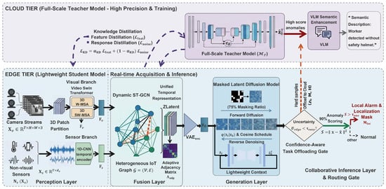
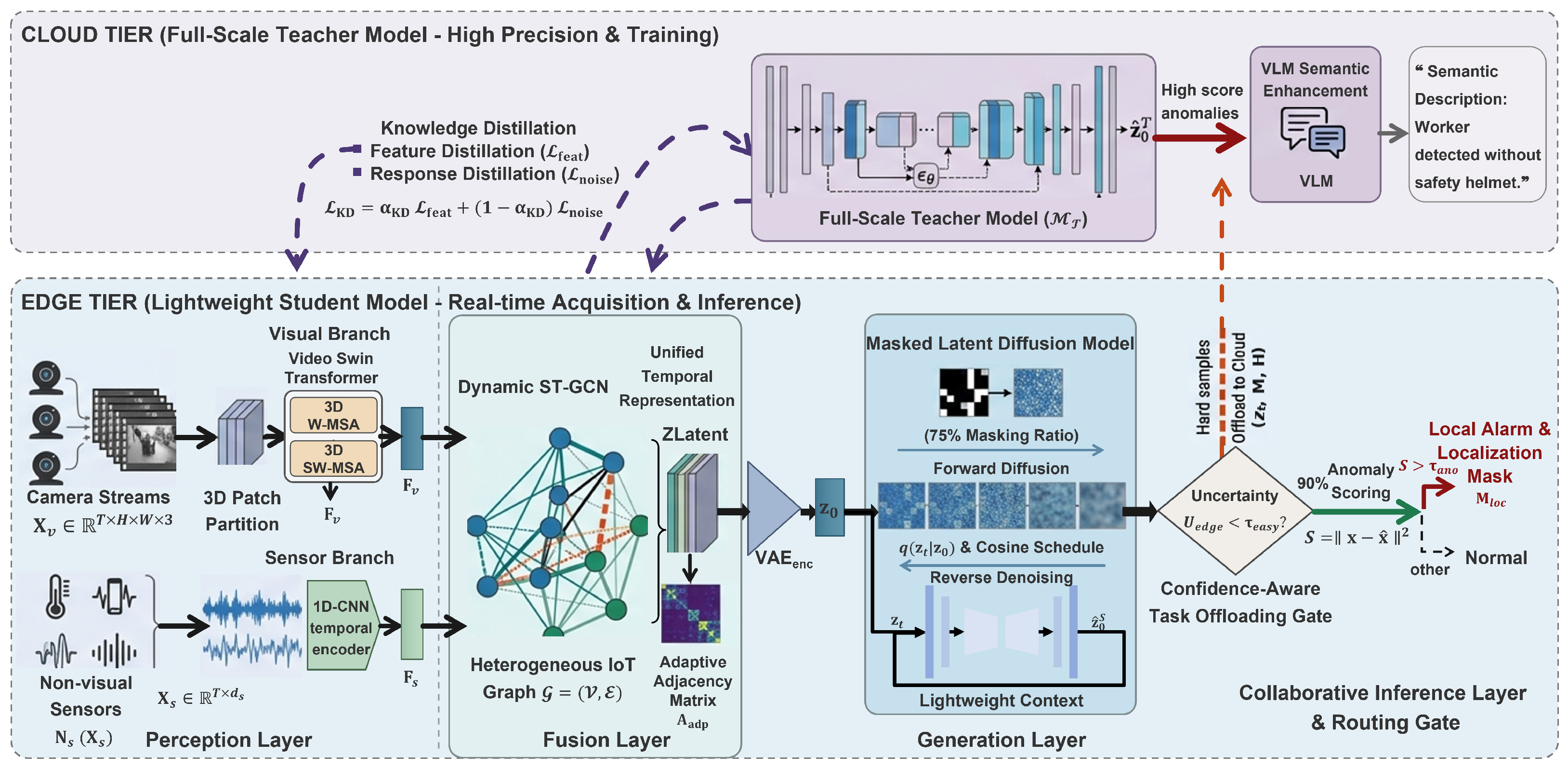
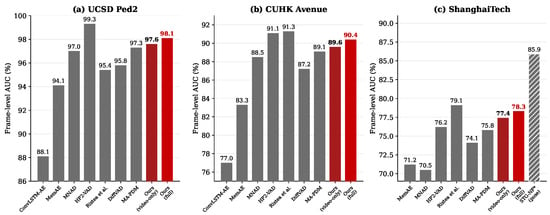
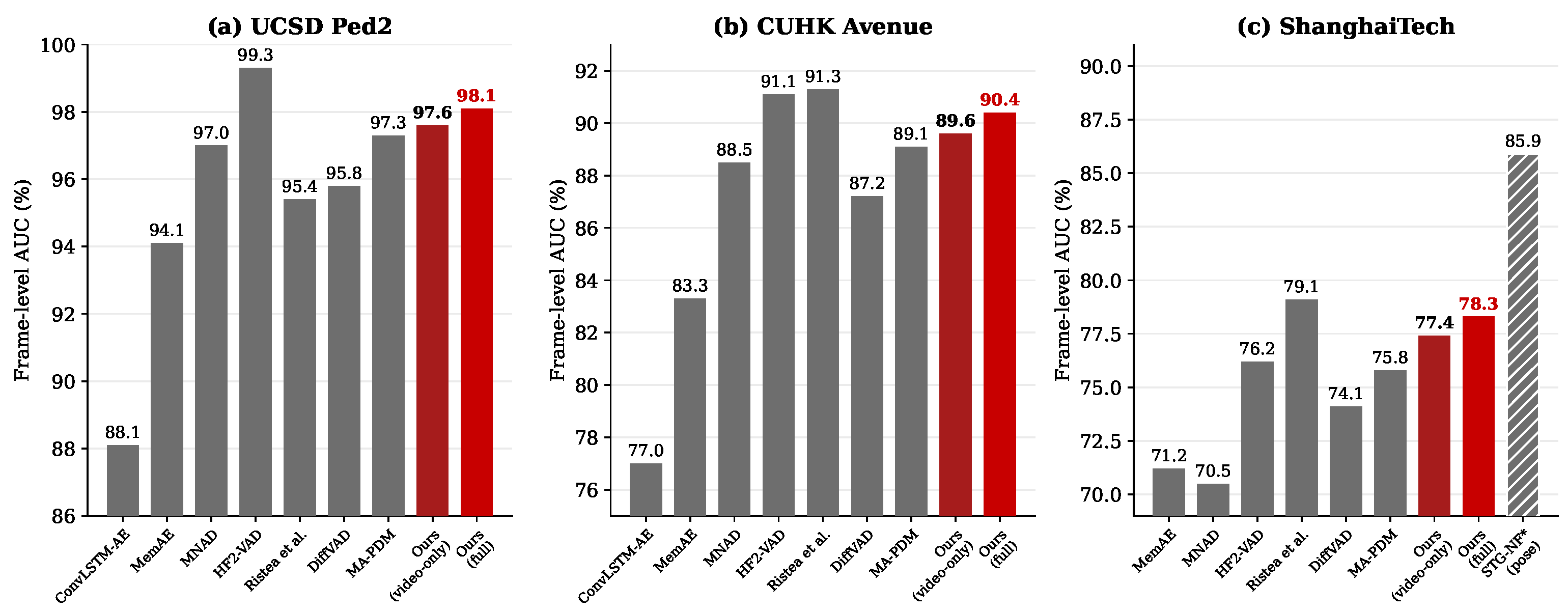
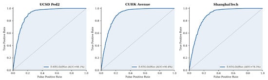
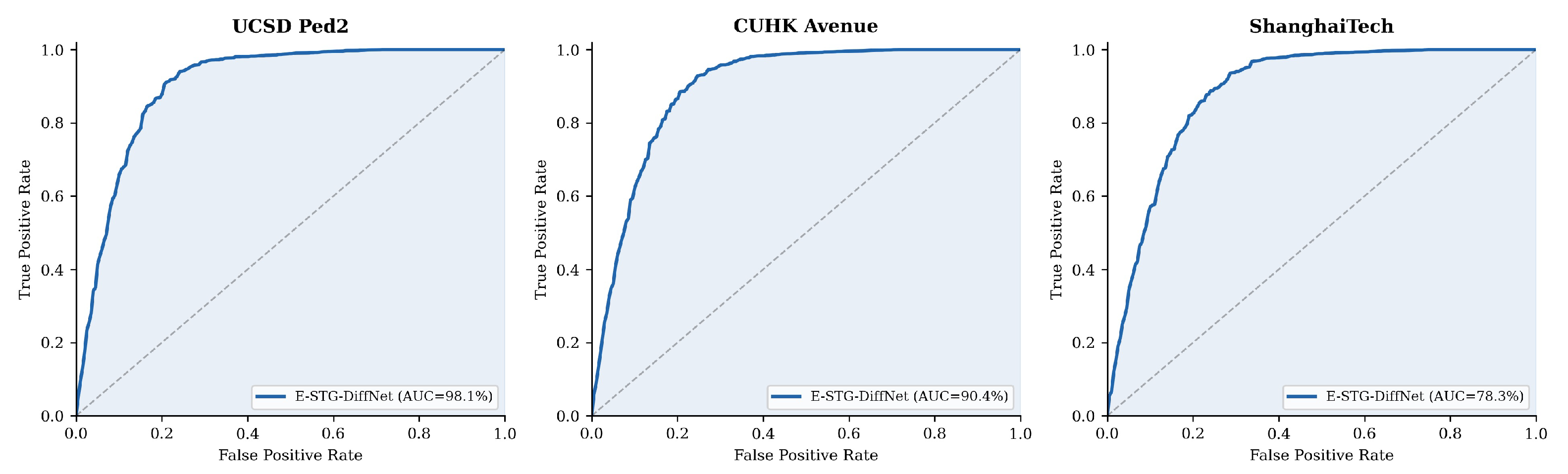
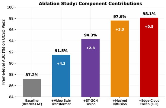
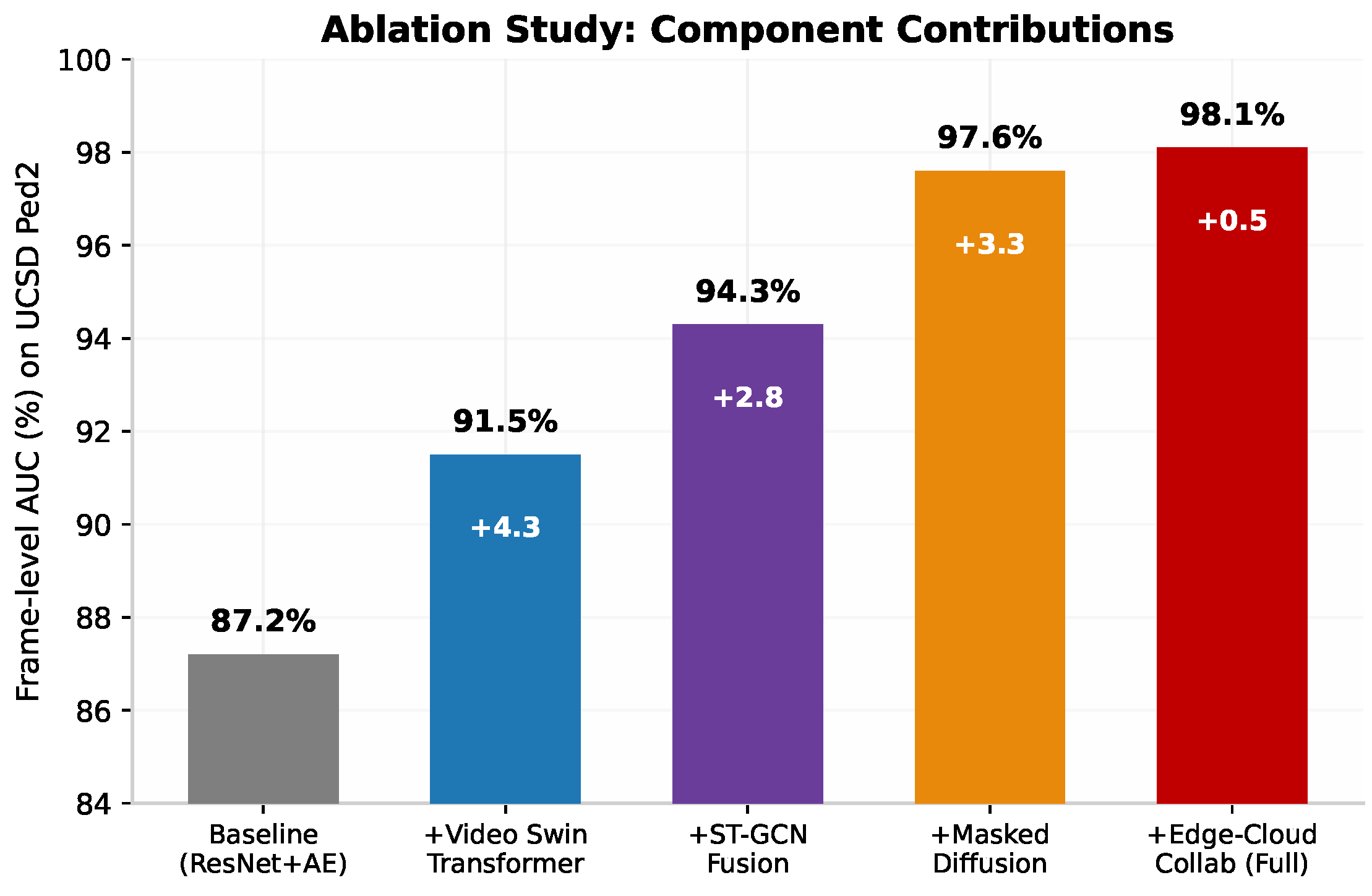
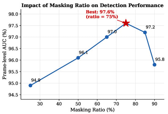
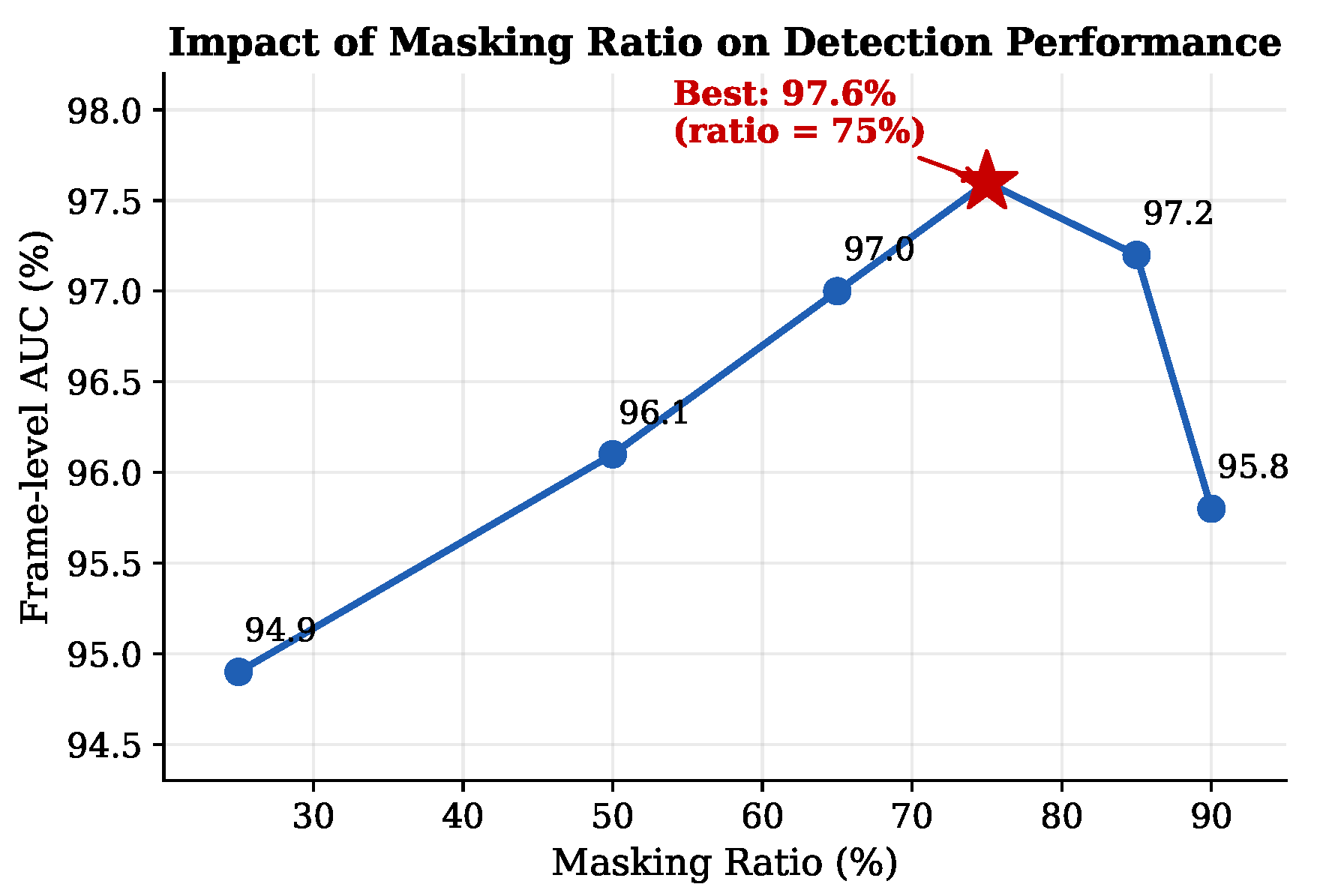
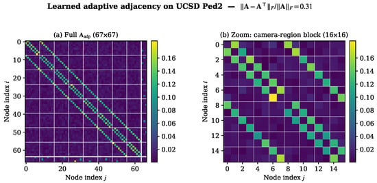
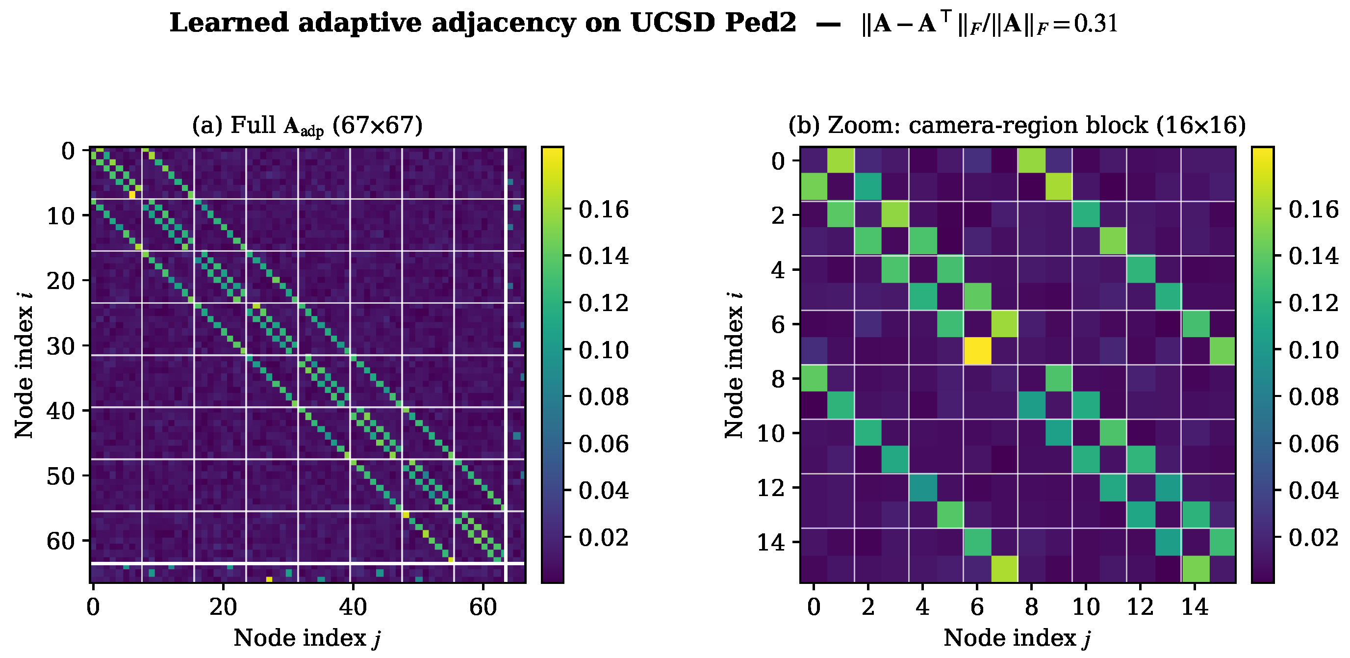
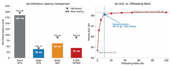
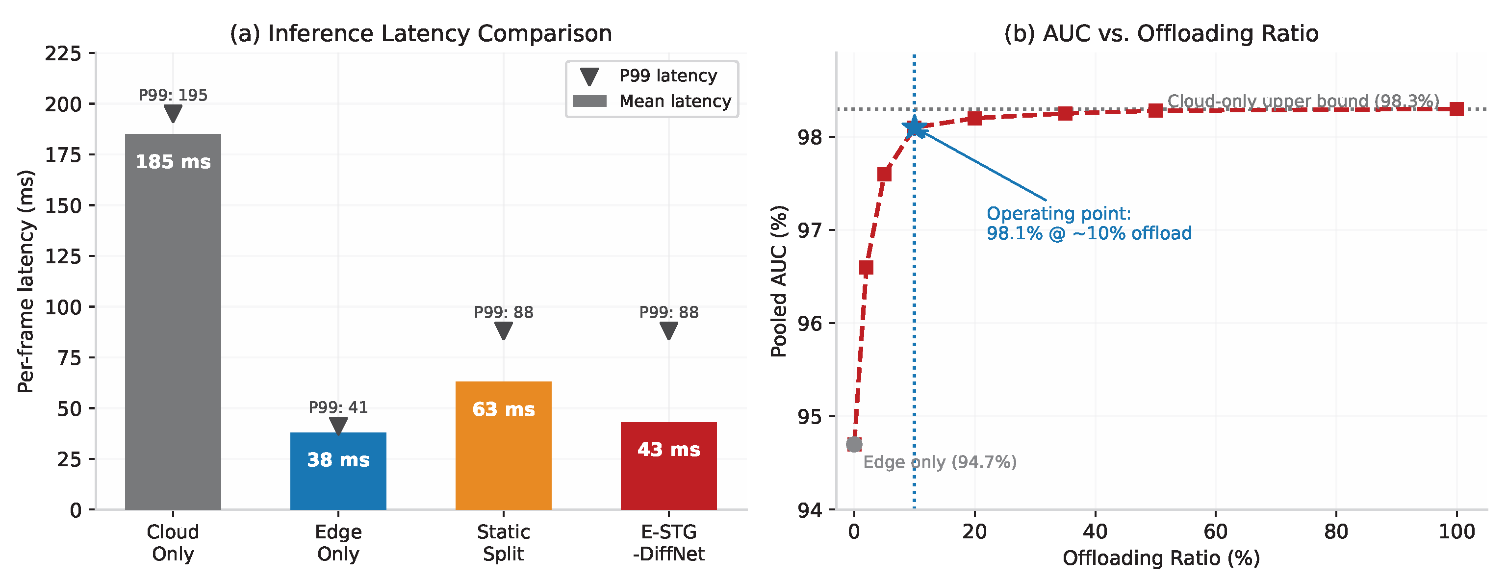
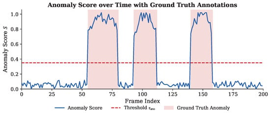
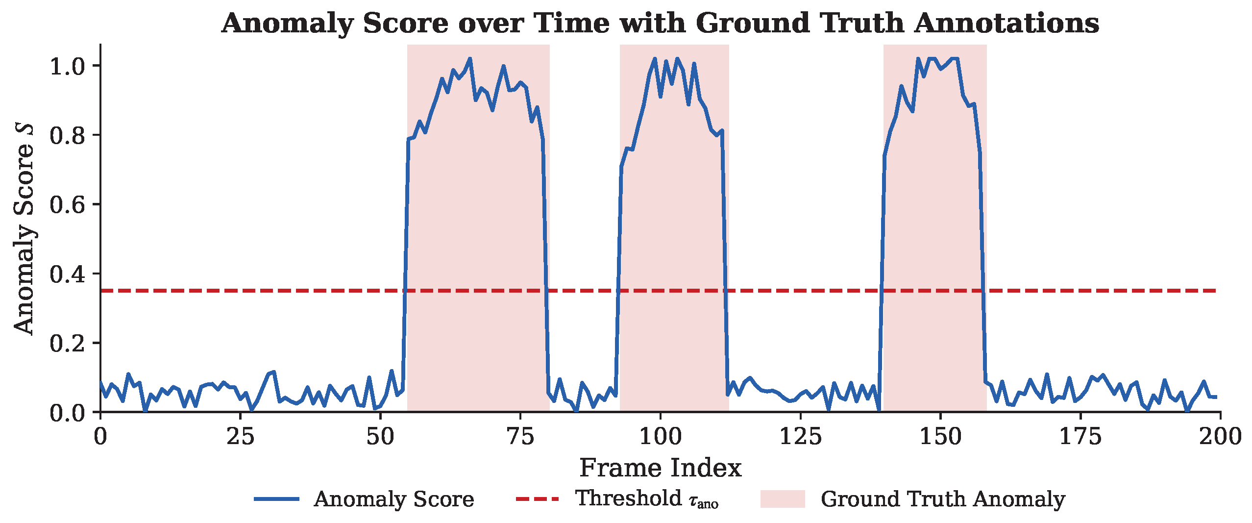
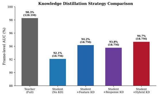
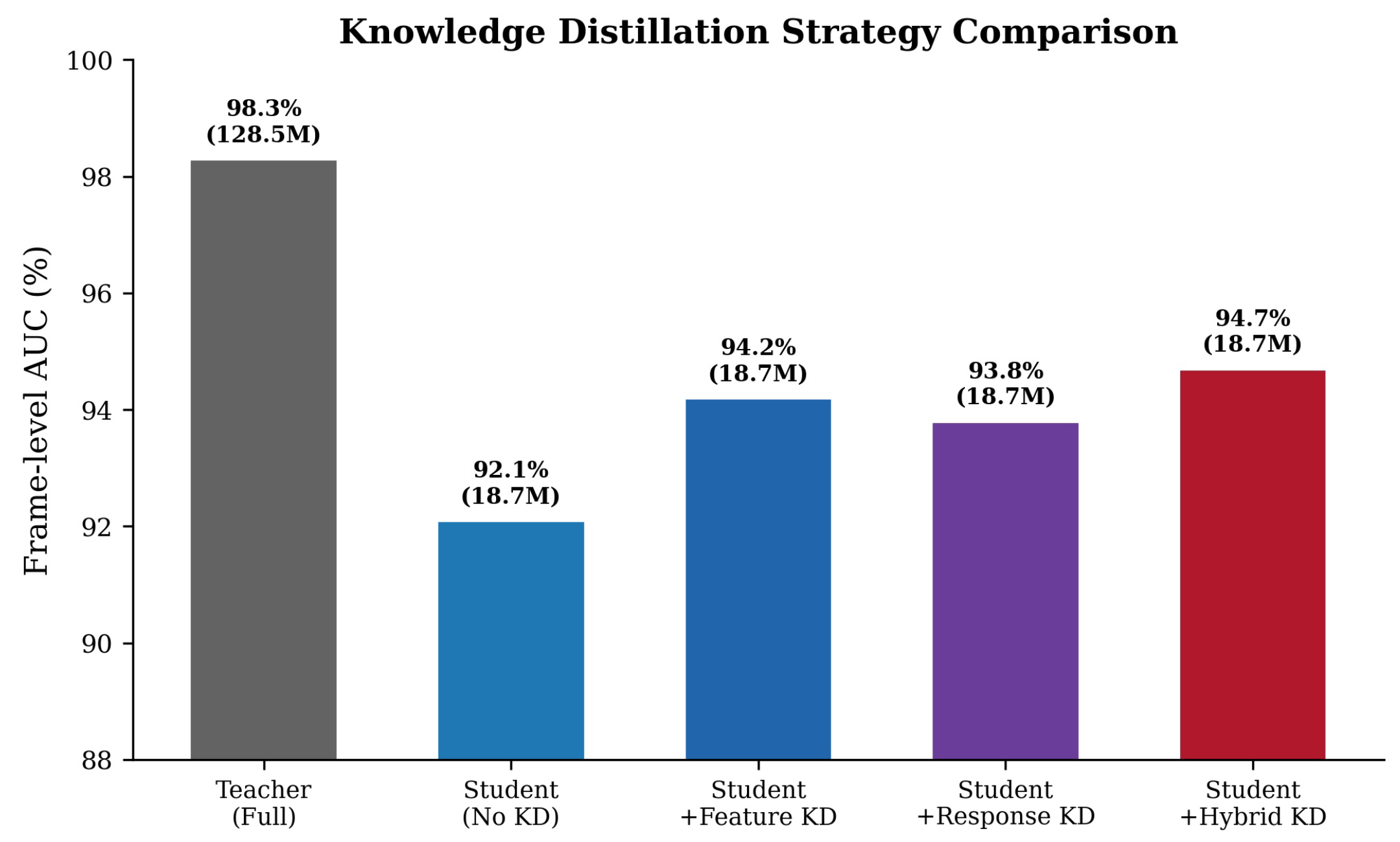
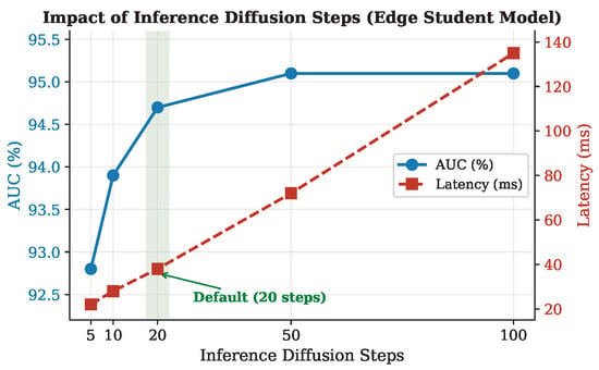
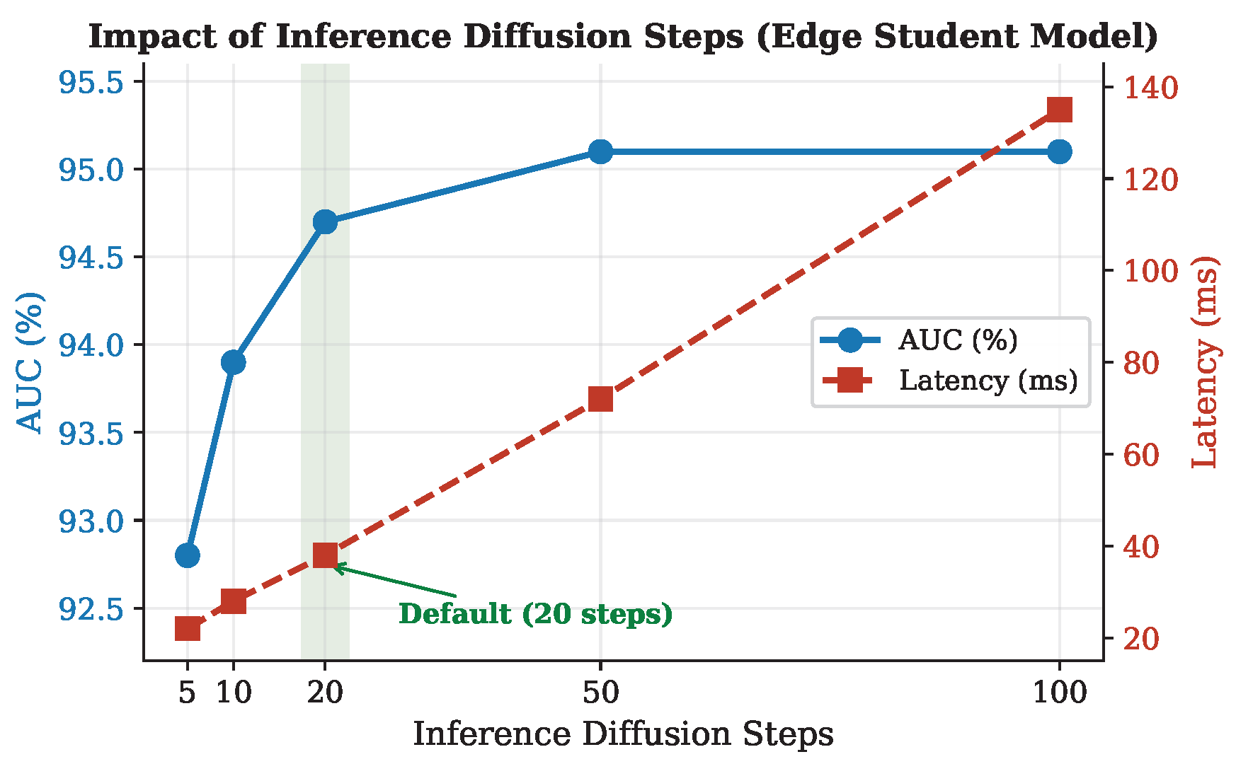

Disclaimer/Publisher’s Note: The statements, opinions and data contained in all publications are solely those of the individual author(s) and contributor(s) and not of MDPI and/or the editor(s). MDPI and/or the editor(s) disclaim responsibility for any injury to people or property resulting from any ideas, methods, instructions or products referred to in the content. |
© 2026 by the authors. Licensee MDPI, Basel, Switzerland. This article is an open access article distributed under the terms and conditions of the Creative Commons Attribution (CC BY) license.