Operational Meaning of the Mandelstam–Tamm Time Scale in a Spin-1/2 Clock. Comment on Georgiev, D.D. Time–Energy Uncertainty Relation in Nonrelativistic Quantum Mechanics. Symmetry 2024, 16, 100

Abstract

Georgiev’s analysis of a freely precessing spin correctly emphasizes that the Mandelstam–Tamm quantity $\mathsf{\Delta }T=\mathsf{\Delta }\widehat{A}/|\mathrm{d}⟨\widehat{A}⟩/\mathrm{d}t|$ is not the variance of a time operator. He concludes, however, that its divergence near the extrema of the clock signal is devoid of physical meaning and that $\mathsf{\Delta }T$ does not disclose how well the system measures the passage of time. For the same projective ${\widehat{\sigma }}_x$ readout, we show that $\mathsf{\Delta }T$ equals the inverse square root of the classical Fisher information in one binary outcome at regular operating points. Its divergence at submaximal-coherence extrema therefore identifies a loss of local sensitivity in the selected readout, not an infinite variance of physical time; a complementary ${\widehat{\sigma }}_y$ measurement remains informative. This interpretation also separates Georgiev’s exactly known tick–tock period from the statistical precision with which a tick can be located. It preserves his warning against a time-operator interpretation while qualifying his stronger conclusion that the Mandelstam–Tamm scale lacks physical content.

1. Scope of the Comment

Georgiev usefully distinguishes the external time parameter from a time operator. He considers the standard Mandelstam–Tamm relation [1], and we agree that this is not a Robertson relation between time and energy as canonical observables. Our target is Georgiev’s narrower inference: he takes the time dependence of the Mandelstam–Tamm scale $\mathsf{\Delta }T$ to disqualify it as a measure of clock quality, and he contrasts its divergence at the extrema of the clock signal with the exactly known interval between consecutive extrema to conclude that it is not a meaningful representation of time.

Georgiev derives the binary outcome probabilities of the spin readout, but does not treat them as a statistical model for estimating t or consider their Fisher information. This omission matters because asking how well a clock measures time is operationally asking how well its outcomes distinguish nearby values of t; Fisher information is the standard local measure of that distinction and controls estimator precision through the Cramér–Rao bound [2]. We therefore read Georgiev’s probabilities as a time-parameterized model, identify $\mathsf{\Delta }T$ with its inverse Fisher sensitivity, compare the selected readout with the quantum information fixed by $\mathsf{\Delta }E$, and then revisit his divergence and tick–tock arguments. This route does not promote time to an observable; it supplies the missing readout-level meaning.

2. The Spin Clock and the Disputed Inference

Georgiev considers the following Hamiltonian, initial state, normalization, and coherence parameter in his Equations (20), (23) and (31):

$$\widehat{H}={\displaystyle \frac{\hslash \omega }{2}}{\widehat{\sigma }}_z,|\mathsf{\Psi }\left(0\right)⟩={\alpha }_1|{\uparrow }_z⟩+{\alpha }_2|{\downarrow }_z⟩,C=2|{\alpha }_1\left|\right|{\alpha }_2|,$$

where $|{\alpha }_1{|}^2+{\left|{\alpha }_2\right|}^2=1$ and C is the ${\ell }_1$ norm of energy coherence. For this pure qubit, C is also the transverse Bloch-vector length. Georgiev’s Equations (29) and (41) give

$$\mathsf{\Delta }\widehat{H}={\displaystyle \frac{1}{2}}\hslash \omega C.$$

and

$$⟨{\widehat{\sigma }}_x⟩=2\left[\mathrm{Re}\left({\alpha }_1{\alpha }_2^{*}\right)\cos \left(\omega t\right)+\mathrm{Im}\left({\alpha }_1{\alpha }_2^{*}\right)\sin \left(\omega t\right)\right],$$

Substitution of his Equations (42) and (44) into the definition in Equation (45) yields Georgiev’s Equation (46):

$$\mathsf{\Delta }T={\displaystyle \frac{\mathsf{\Delta }{\widehat{\sigma }}_x}{\left|\frac{\mathrm{d}}{\mathrm{d}t}⟨{\widehat{\sigma }}_x⟩\right|}}={\displaystyle \frac{\left|{\alpha }_1^2{\mathrm{e}}^{-\mathrm{i}\omega t}-{\alpha }_2^2{\mathrm{e}}^{\mathrm{i}\omega t}\right|}{2\omega \left|\mathrm{Re}\left({\alpha }_1{\alpha }_2^{*}\right)\sin \left(\omega t\right)-\mathrm{Im}\left({\alpha }_1{\alpha }_2^{*}\right)\cos \left(\omega t\right)\right|}}.$$

Here $\omega >0$ denotes the angular frequency. For convenience let

$${\alpha }_1{\alpha }_2^{*}=\left|{\alpha }_1{\alpha }_2\right|{\mathrm{e}}^{\mathrm{i}\varphi },\vartheta =\omega t-\varphi .$$

Equations (41)–(44) of Ref. [3] then give

$$\begin{array}{cc}\hfill \mathsf{\Delta }{\widehat{\sigma }}_x& =\left|{\alpha }_1^2{\mathrm{e}}^{-\mathrm{i}\omega t}-{\alpha }_2^2{\mathrm{e}}^{\mathrm{i}\omega t}\right|=\sqrt{1-{⟨{\widehat{\sigma }}_x⟩}^2}=\sqrt{1-C^2{\cos }^2\vartheta },\hfill \\ \hfill ⟨{\widehat{\sigma }}_x⟩& =C\cos \vartheta ,\hfill \\ \hfill \left|{\displaystyle \frac{\mathrm{d}}{\mathrm{d}t}}⟨{\widehat{\sigma }}_x⟩\right|& =\omega C\left|\sin \vartheta \right|.\hfill \end{array}$$

Note that the time argument of $⟨{\widehat{\sigma }}_x⟩$ is suppressed in the notation, although $⟨{\widehat{\sigma }}_x⟩$ remains time-dependent.

Hence

$$\mathsf{\Delta }T={\displaystyle \frac{\sqrt{1-C^2{\cos }^2\vartheta }}{\omega C\left|\sin \vartheta \right|}}.$$

(1)

Equation (1) is an algebraic rewriting of Georgiev’s Equation (46). For $0<C<1$, it diverges at $\vartheta =k\pi$, where the signal is extremal. For $C=1$, the numerator and denominator cancel away from those points, yielding $1/\omega$, as in his Equation (48); exactly at an extremum, the defining ratio is $0/0$ and only its interior limit is finite. These algebraic facts are not in dispute. The issue is their interpretation.

3. The Time Scale Is an Inverse Fisher Sensitivity

The starting point of our analysis is Georgiev’s Equation (51) [3], which expresses the instantaneous standard deviation of an observable $\widehat{A}$ in terms of the rate of change of its expectation value and the characteristic time $\mathsf{\Delta }T\left(t\right)$,

$$\mathsf{\Delta }\widehat{A}\left(t\right)=\left|{\displaystyle \frac{\mathrm{d}}{\mathrm{d}t}}⟨\widehat{A}⟩\right|\left(t\right)\mathsf{\Delta }T\left(t\right).$$

(2)

Immediately after Equation (2), Georgiev interprets $\mathsf{\Delta }T\left(t\right)$ as an instantaneous “hypothetical time duration that would have been taken by the quantum observable moving with a constant speed equal to the instantaneous rate of change $\left|{\displaystyle \frac{\mathrm{d}}{\mathrm{d}t}}⟨\widehat{A}⟩\right|\left(t\right)$ until a distance equal to the instantaneous standard deviation $\mathsf{\Delta }\widehat{A}\left(t\right)$ would have been traversed.” ([3], p. 9) Because the signal accelerates and decelerates, he concludes that $\mathsf{\Delta }T\left(t\right)$ does not disclose how well the system measures the passage of time, in contrast with the constant $\mathsf{\Delta }E$. We now apply the estimation route stated above to show why that conclusion is too strong.

A projective measurement of ${\widehat{\sigma }}_x$ returns $m=\pm 1$, not the expectation value $⟨{\widehat{\sigma }}_x⟩$ itself. Georgiev’s projector probabilities in Equations (39) and (40) can be written as

$$p_m\left(t\right)={\displaystyle \frac{1}{2}}+m\left[\mathrm{Re}\left({\alpha }_1{\alpha }_2^{*}\right)\cos \left(\omega t\right)+\mathrm{Im}\left({\alpha }_1{\alpha }_2^{*}\right)\sin \left(\omega t\right)\right]={\displaystyle \frac{1+m⟨{\widehat{\sigma }}_x⟩}{2}},m=\pm 1.$$

Whenever $0<p_m<1$, the classical Fisher information per projective measurement about the parameter t is

$$\begin{array}{cc}\hfill F_x\left(t\right)& =\sum _{m=\pm 1}{\displaystyle \frac{{\left[\frac{\mathrm{d}}{\mathrm{d}t}{p}_m\left(t\right)\right]}^2}{p_m\left(t\right)}}={\displaystyle \frac{{\left[\frac{\mathrm{d}}{\mathrm{d}t}⟨{\widehat{\sigma }}_x⟩\right]}^2}{1-{⟨{\widehat{\sigma }}_x⟩}^2}}\hfill \\ \hfill & ={\displaystyle \frac{{\omega }^2{C}^2{\sin }^2\vartheta }{1-C^2{\cos }^2\vartheta }}.\hfill \end{array}$$

(3)

The Fisher information quantifies the local statistical distinguishability of the outcome distributions at neighbouring values of t [2]. A large $F_x\left(t\right)$ means that a small change of time appreciably changes the probabilities $p_m\left(t\right)$; $F_x\left(t\right)=0$ means that this selected readout is insensitive to time to first order. The Fisher information is calculated from the time-dependent outcome probabilities of a specified measurement. It is therefore a property of the statistical readout model $p_m\left(t\right)$, not the expectation value of a quantum observable and not, by itself, the variance of a time estimator.

At a locally identifiable operating point, where $F_x\left(t\right)>0$, a binary Pauli outcome obeys $\mathsf{\Delta }{\widehat{\sigma }}_x=\sqrt{1-{⟨{\widehat{\sigma }}_x⟩}^2}$ and Equations (1) and (3) give the exact identity

$$\begin{array}{|c|}\hline \mathsf{\Delta }T\left(t\right)={\displaystyle \frac{1}{\sqrt{F_x\left(t\right)}}}\\ \hline\end{array}.$$

(4)

Thus Georgiev’s Equation (51) has a direct statistical meaning for his chosen readout: $\mathsf{\Delta }T$ is its inverse local sensitivity to a change of t. It is neither the variance of a time operator nor the elapsed duration of a single run. Its phase dependence instead describes how the information about t available from the ${\widehat{\sigma }}_x$ measurement changes during the spin precession.

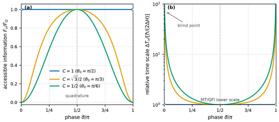
At a submaximal-coherence extremum, $0<C<1$ and $\vartheta =k\pi$, one has ${\displaystyle \frac{\mathrm{d}}{\mathrm{d}t}}{p}_m=F_x=0$. The divergence $\mathsf{\Delta }T=\infty$ expresses loss of first-order sensitivity; it is not an infinite variance of physical time. The probabilities of the ${\widehat{\sigma }}_x$ outcomes change only to second order in a small displacement from the extremum and are identical for opposite displacements.

Georgiev is nevertheless right that $\mathsf{\Delta }E$ has a different status. To make this distinction precise, we introduce the quantum Fisher information $F_Q$. At a fixed value of t, $F_Q$ is the maximum classical Fisher information obtainable from the time-dependent quantum state by optimizing over all possible measurements. It therefore quantifies the greatest local sensitivity to t available in the state before a particular readout is selected [4,5].

For the pure state undergoing Georgiev’s unitary evolution,

$$F_Q=4\left(⟨\dot{\mathsf{\Psi }}|\dot{\mathsf{\Psi }}⟩-{\left|⟨\mathsf{\Psi }|\dot{\mathsf{\Psi }}⟩\right| }^2\right)={\displaystyle \frac{4{\left(\mathsf{\Delta }\widehat{H}\right)}^2}{{\hslash }^2}}={\omega }^2{C}^2$$

(5)

where $|\dot{\mathsf{\Psi }}⟩\equiv {\displaystyle \frac{\mathrm{d}}{\mathrm{d}t}}|\mathsf{\Psi }\left(t\right)⟩$.

For mixed states undergoing unitary evolution, one generally has $F_Q\le 4{\left(\mathsf{\Delta }\widehat{H}\right)}^2/{\hslash }^2$, and the inequality can be strict. Returning to Georgiev’s pure-state model, at regular operating points one finds

$$F_Q-F_x={\displaystyle \frac{{\omega }^2{C}^2(1-C^2){\cos }^2\vartheta }{1-C^2{\cos }^2\vartheta }}\ge 0.$$

(6)

The nonnegative difference $F_Q-F_x$ quantifies the local timing information available in the quantum state but not accessed by the selected ${\widehat{\sigma }}_x$ measurement. When $F_x=F_Q$, the measurement is locally optimal; when $F_x=0<F_Q$, the state remains sensitive to t, but the ${\widehat{\sigma }}_x$ measurement fails to reveal that sensitivity to first order.

Consequently, at regular operating points with $F_x\left(t\right)>0$,

$$\mathsf{\Delta }T\mathsf{\Delta }\widehat{H}={\displaystyle \frac{\hslash }{2}}{\displaystyle \frac{\sqrt{1-C^2{\cos }^2\vartheta }}{\left|\sin \vartheta \right|}}={\displaystyle \frac{\hslash }{2}}\sqrt{{\displaystyle \frac{F_Q}{F_x}}}\ge {\displaystyle \frac{\hslash }{2}}.$$

(7)

Thus the Mandelstam–Tamm inequality is the information hierarchy $F_x\le F_Q$: the selected readout cannot contain more information about the time translation than the state itself. In this precise sense, the constant $\mathsf{\Delta }E$ fixes the best sensitivity allowed by the state, while the phase-dependent $\mathsf{\Delta }T$ describes how much of that sensitivity Georgiev’s selected ${\widehat{\sigma }}_x$ measurement actually accesses. The two quantities answer different questions, so the variability of one does not make it meaningless.

For N independently and identically prepared states, Fisher information adds. At a locally identifiable regular point with $F_x\left(t\right)>0$, any locally unbiased estimator therefore obeys

$$\mathrm{Var}\left(\widehat{t}\right)\ge {\displaystyle \frac{1}{N{F}_x\left(t\right)}}={\displaystyle \frac{\mathsf{\Delta }{T}^2}{N}}.$$

(8)

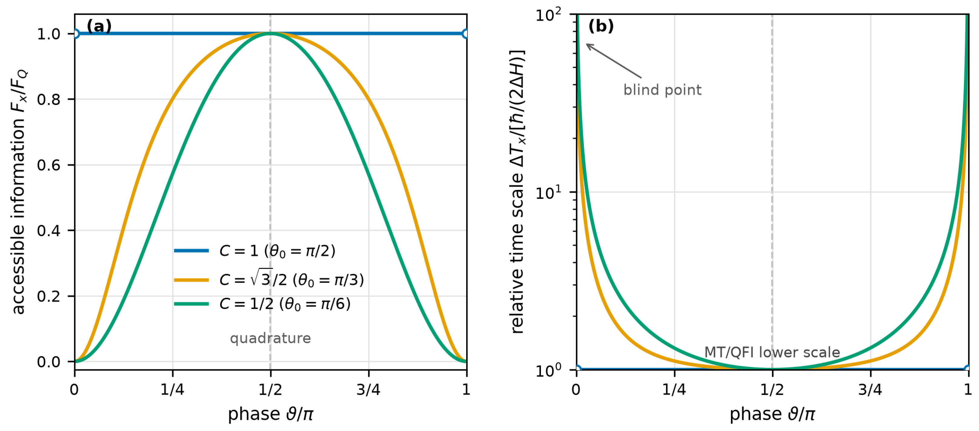
Thus $\mathsf{\Delta }T/\sqrt{N}$ is the local Cramér–Rao sensitivity scale, which can be approached asymptotically by an efficient estimator under the usual regularity conditions. The corresponding statement about estimation uncertainty is therefore expressed by Equation (8), not by $\mathsf{\Delta }T$ alone. Finite samples, estimator bias, and global ambiguities arising from the periodicity of the signal require separate treatment [6,7]. Figure 1 summarizes the accessible information and the corresponding relative time scale over one half-period.

Figure 1. Temporal sensitivity of Georgiev’s ${\widehat{\mathsf{\sigma }}}_{\mathit{x}}$ clock. We take ${\mathsf{\alpha }}_{\mathbf{1}}{\mathsf{\alpha }}_{\mathbf{2}}^{*}$ real and positive, so that $\mathsf{\vartheta }=\mathsf{\omega }\mathit{t}$. Panel (a) shows the accessible fraction ${\mathit{F}}_{\mathit{x}}/{\mathit{F}}_{\mathit{Q}}$; panel (b) shows $\mathsf{\Delta }\mathit{T}/[\hslash /\left(\mathbf{2}\mathsf{\Delta }\widehat{\mathit{H}}\right)]=\sqrt{{\mathit{F}}_{\mathit{Q}}/{\mathit{F}}_{\mathit{x}}}$. At $\mathsf{\omega }\mathit{t}=\mathsf{\pi }/\mathbf{2}$, the maximum-slope (quadrature) point, the ${\widehat{\mathsf{\sigma }}}_{\mathit{x}}$ readout attains the quantum Fisher-information bound ${\mathit{F}}_{\mathit{x}}={\mathit{F}}_{\mathit{Q}}$ for every $\mathit{C}>\mathbf{0}$. For $\mathit{C}<\mathbf{1}$, ${\mathit{F}}_{\mathit{x}}$ vanishes at the extrema and the relative time scale diverges. Open circles for $\mathit{C}=\mathbf{1}$ denote interior limits at the nonregular endpoints.

4. Divergences and Georgiev’s Tick–Tock Argument

Georgiev draws his strongest conclusion after Equations (52)–(54). At a maximum or minimum of $⟨{\widehat{\sigma }}_x⟩$, $\mathsf{\Delta }T$ diverges for $C<1$, whereas the interval between consecutive extrema is exactly $\delta t=\pi /\omega$. He argues that $\mathsf{\Delta }T$ would therefore “wrongly predict” an infinite standard deviation of time and concludes that it is not a meaningful representation of time. This comparison puts together two different quantities.

For $0<C<1$ at $\vartheta =k\pi$, $F_x=0$ while $F_Q>0$. The divergence of $\mathsf{\Delta }T$ means that the selected ${\widehat{\sigma }}_x$ measurement has no first-order sensitivity to a small time displacement from the extremum. It does not imply that external time has a statistical variance, nor does it make the known period $\pi /\omega$ uncertain. Estimation exactly there is nonregular because the leading change of the ${\widehat{\sigma }}_x$ outcome probabilities is quadratic and does not determine on which side of the extremum the system lies.

The complementary readout has

$$F_y\left(t\right)={\displaystyle \frac{{\omega }^2{C}^2{\cos }^2\vartheta }{1-C^2{\sin }^2\vartheta }}.$$

At an extremum of $⟨{\widehat{\sigma }}_x⟩$, $F_y=F_Q$; conversely, the ${\widehat{\sigma }}_x$ readout is optimal at $\cos \vartheta =0$ for every $C>0$. Thus the divergence identified by Georgiev is readout-specific, not a disappearance of temporal information from the state. Operationally, a clock can switch to the complementary quadrature near a ${\widehat{\sigma }}_x$ extremum; without prior phase knowledge, the same idea requires a local or adaptive measurement strategy.

Georgiev’s Equations (52)–(54) relate the energy gap to the separation between consecutive “tick” and “tock” extrema:

$$\begin{array}{cc}\hfill \omega & ={\displaystyle \frac{|E_1-E_2|}{\hslash }},\hfill \\ \hfill \delta t& =|t_2-t_1|={\displaystyle \frac{\pi }{\omega }},\hfill \\ \hfill \delta E\delta t& ={\displaystyle \frac{h}{2}},\delta E=|E_1-E_2|.\hfill \end{array}$$

These relations fix the separation between ideal extrema of a signal whose frequency is already known. They do not determine the statistical precision with which an extremum can be located from measurement outcomes. For $C<1$, an extremal expectation value is $⟨{\widehat{\sigma }}_x⟩=\pm C$, whereas one projective outcome remains random, $m=\pm 1$. Locating a tick therefore requires an ensemble of identically prepared spins, repeated runs, or prior synchronization. Even for $C=1$, the endpoint model is nonregular and the ${\widehat{\sigma }}_x$ readout does not distinguish the two signs of a displacement. Periodicity also leaves the cycle number undetermined without coarse timing information. Hence Georgiev’s Equation (53) is fully compatible with a divergent local ${\widehat{\sigma }}_x$-readout scale: the former is a calibrated half-period, while the latter describes the loss of first-order timing information in a specified measurement.

5. Conclusions

Georgiev is correct that $\mathsf{\Delta }T$ is neither a time-operator variance nor an elapsed time produced by a single run. His stronger inference does not follow. In his own ${\widehat{\sigma }}_x$ experiment, $\mathsf{\Delta }T$ is the inverse Fisher sensitivity at regular operating points. Its phase dependence describes the performance of the selected readout, and its divergence identifies a locally blind quadrature; neither conflicts with the exactly calibrated half-period $\delta t=\pi /\omega$. A complementary quadrature can retain the information that the ${\widehat{\sigma }}_x$ readout loses. These qualifications preserve Georgiev’s conceptual warning while replacing physical meaninglessness with a precise, measurement-dependent operational meaning.

References

- Mandelstam, L.; Tamm, I. The Uncertainty Relation between Energy and Time in Non-Relativistic Quantum Mechanics. J. Phys. (USSR) 1945, 9, 249–254. [Google Scholar]
- Paris, M.G.A. Quantum Estimation for Quantum Technology. Int. J. Quantum Inf. 2009, 7, 125–137. [Google Scholar] [CrossRef] [Scilit]
- Georgiev, D.D. Time–Energy Uncertainty Relation in Nonrelativistic Quantum Mechanics. Symmetry 2024, 16, 100. [Google Scholar] [CrossRef] [Scilit]
- Braunstein, S.L.; Caves, C.M. Statistical Distance and the Geometry of Quantum States. Phys. Rev. Lett. 1994, 72, 3439–3443. [Google Scholar] [CrossRef] [Scilit]
- Braunstein, S.L.; Caves, C.M.; Milburn, G.J. Generalized Uncertainty Relations: Theory, Examples, and Lorentz Invariance. Ann. Phys. 1996, 247, 135–173. [Google Scholar] [CrossRef] [Scilit]
- Tsang, M. Ziv–Zakai Error Bounds for Quantum Parameter Estimation. Phys. Rev. Lett. 2012, 108, 230401. [Google Scholar] [CrossRef] [Scilit]
- Meyer, J.J.; Khatri, S.; Stilck França, D.; Eisert, J.; Faist, P. Quantum Metrology in the Finite-Sample Regime. PRX Quantum 2025, 6, 030336. [Google Scholar] [CrossRef] [Scilit]
Disclaimer/Publisher’s Note: The statements, opinions and data contained in all publications are solely those of the individual author(s) and contributor(s) and not of MDPI and/or the editor(s). MDPI and/or the editor(s) disclaim responsibility for any injury to people or property resulting from any ideas, methods, instructions or products referred to in the content. |
© 2026 by the author. Licensee MDPI, Basel, Switzerland. This article is an open access article distributed under the terms and conditions of the Creative Commons Attribution (CC BY) license.