


Abstract
Financial time series are characterized by high volatility, nonstationarity, nonlinear dynamics, and multiscale fluctuations, which pose significant challenges to accurate stock price forecasting. In multivariate financial forecasting, financial variables may exhibit symmetric and asymmetric characteristics in their temporal fluctuations and structural dependencies across different time scales. Understanding these characteristics is relevant to the analysis of symmetry and asymmetry in financial time series. Modeling multiscale temporal patterns and inter-variable dependencies is therefore important for improving forecasting performance. To address these challenges, this study proposes a hybrid CEEMDAN–IGOA–TCN–iTransformer framework for multivariate stock price prediction. First, Complete Ensemble Empirical Mode Decomposition with Adaptive Noise (CEEMDAN) is employed to decompose financial time series into intrinsic mode functions and residual components, facilitating multiscale feature extraction. Second, a population-based hyperparameter optimization procedure is employed to select key model hyperparameters based on validation performance. Third, a TCN–iTransformer architecture is constructed, in which the Temporal Convolutional Network (TCN) extracts local temporal features and multiscale patterns, while the iTransformer models dependencies among financial input variables through its inverted attention mechanism. Finally, the extracted features are integrated to generate the predicted stock closing price. Experiments were conducted on three Chinese A-share stock datasets, representing Ping An Insurance, BOE Technology Group, and Arcplus Group. The proposed framework achieved test-set RMSE values of 0.8987, 0.0656, and 0.6717, respectively, with a corresponding arithmetic mean RMSE of 0.5453 across the three datasets. Comparative experiments and ablation studies were conducted to evaluate the forecasting performance and contributions of the framework’s components. The findings indicate that the proposed approach can provide accurate one-step-ahead closing-price predictions under the investigated experimental conditions, while its performance and generalizability remain dependent on the characteristics of the evaluated datasets.
1. Introduction
Financial time series forecasting has long been one of the most challenging and important research topics in quantitative finance, financial engineering, and artificial intelligence [1,2]. Accurate prediction of stock prices and market movements plays a crucial role in portfolio optimization, risk management, and investment decision-making [3]. However, financial markets are characterized by high volatility, nonlinearity, nonstationarity, and noise, making it extremely difficult to model the underlying dynamics of asset prices effectively [4]. The efficient market hypothesis further suggests that market prices incorporate available information rapidly, thereby increasing the complexity of financial forecasting tasks [5].
Traditional statistical approaches, such as the Autoregressive Integrated Moving Average (ARIMA) and Generalized Autoregressive Conditional Heteroskedasticity (GARCH) models, have been extensively applied to financial forecasting problems [6]. Although these methods perform well under specific assumptions, they generally struggle to capture the nonlinear dependencies and complex temporal structures inherent in financial time series [7]. With the rapid development of machine learning and deep learning techniques, various neural network models, including Recurrent Neural Networks (RNN), Long Short-Term Memory (LSTM), and Gated Recurrent Unit (GRU), have been introduced into financial forecasting [8]. These methods significantly improve prediction performance by learning nonlinear patterns directly from historical data [9]. Nevertheless, recurrent architectures often suffer from gradient vanishing, limited parallel computation capability, and difficulties in modeling long-range dependencies [10].
Recently, Transformer-based architectures have demonstrated remarkable success in sequence modeling tasks [11]. Owing to their self-attention mechanisms and parallel processing capabilities, Transformers can effectively capture long-term dependencies and global contextual information [12]. Consequently, numerous Transformer variants, including Informer, Autoformer, PatchTST, and iTransformer, have been successfully applied to financial forecasting problems [13,14]. Among them, iTransformer achieves superior performance by modeling variables as independent tokens and learning inter-variable dependencies through an inverted attention mechanism [15]. Despite these advances, existing forecasting frameworks still face several critical challenges, including the presence of nonstationary and noisy financial signals, the sensitivity of deep learning models to hyperparameter configurations, and the insufficient modeling of local temporal dynamics. These limitations motivate the development of more robust hybrid forecasting frameworks.
First, raw financial time series exhibit strong nonstationarity and contain substantial noise components, which may degrade the learning capability of deep neural networks [16]. To address this issue, signal decomposition methods have been widely adopted [17]. In particular, Complete Ensemble Empirical Mode Decomposition with Adaptive Noise (CEEMDAN) has shown superior ability in decomposing complex financial sequences into several intrinsic mode functions with different frequency characteristics [18]. By separating high-frequency noise and low-frequency trend information, CEEMDAN effectively improves the predictability of financial time series and has been successfully integrated with LSTM, Informer, and other forecasting models [19]. This multiscale decomposition strategy provides more informative and structured inputs for subsequent forecasting models.
Second, existing Transformer architectures often focus primarily on global dependency modeling while neglecting local temporal patterns and multi-scale dynamics that are essential in financial markets [20,21]. Temporal Convolutional Networks (TCNs), with their causal convolution and dilated convolution mechanisms, provide an effective way to capture local temporal dependencies and multiscale features [22]. Therefore, integrating TCN with Transformer architectures enables complementary modeling of both local temporal dynamics and global dependency relationships, thereby enabling more comprehensive temporal feature representation for financial forecasting tasks [23].
Third, since the predictive performance of deep learning models is highly sensitive to hyperparameter configurations, efficient hyperparameter optimization has become an essential component for improving forecasting accuracy and model generalization. Metaheuristic optimization algorithms provide an efficient alternative for hyperparameter optimization [24]. The Grasshopper Optimization Algorithm (GOA) is a swarm intelligence optimization method that has demonstrated excellent global search capability and robustness in solving complex optimization problems [25]. However, the original GOA suffers from slow convergence and a tendency to become trapped in local optima [26]. To address these limitations, several improved variants of GOA have been proposed by incorporating strategies such as Levy flight, opposition-based learning, chaotic initialization, and nonlinear control mechanisms [27]. Among them, the Improved Grasshopper Optimization Algorithm (IGOA) has exhibited superior optimization performance and has been successfully applied to parameter optimization problems in forecasting models [28]. Therefore, integrating the Improved Grasshopper Optimization Algorithm into deep learning forecasting frameworks provides an effective strategy for automatically searching the optimal hyperparameter combinations, improving convergence efficiency, avoiding local optima, and enhancing model generalization [29].
From the perspective of symmetry, financial time series may exhibit both symmetric and asymmetric characteristics in their temporal fluctuations and inter-variable relationships. Symmetry generally refers to the preservation of certain structural properties under specified transformations, whereas asymmetry indicates that such properties are not preserved. In financial markets, upward and downward price movements may exhibit different volatility characteristics, and the predictive relationships among financial variables may vary across market conditions and temporal scales. These characteristics highlight the importance of investigating structural relationships in multivariate financial forecasting. Although the proposed framework does not explicitly impose symmetry constraints, its multiscale decomposition and variable-wise attention mechanisms provide a means of learning complex temporal and inter-variable dependencies that may contain symmetric or asymmetric patterns.
Although substantial progress has been achieved, existing studies generally address only one or two aspects of financial forecasting. To the best of our knowledge, few existing studies have combined CEEMDAN, an improved swarm intelligence optimization algorithm, TCN, and iTransformer into a unified hybrid forecasting framework for stock price prediction. Consequently, there remains a need for an end-to-end hybrid architecture capable of jointly addressing the nonstationarity, multiscale characteristics, and complex temporal dependencies of financial time series. Motivated by these observations, this study proposes a novel hybrid forecasting framework termed CEEMDAN–IGOA–TCN–iTransformer for financial time series prediction. The proposed framework consists of three sequential stages: causal signal decomposition, hyperparameter optimization, and hybrid closing-price forecasting. First, CEEMDAN is employed to decompose the raw stock price series into multiple intrinsic mode functions, thereby mitigating nonstationarity and enhancing multiscale feature representation. Second, the Improved Grasshopper Optimization Algorithm (IGOA) is employed to automatically optimize the key hyperparameters of the forecasting framework based on validation performance. Third, a hybrid TCN–iTransformer architecture is constructed, in which TCN captures local temporal patterns and multiscale dependencies, while iTransformer models long-range inter-variable relationships through its inverted attention mechanism. Finally, the model directly predicts the next-day closing price based on the learned temporal features and inter-variable dependencies.
The primary contributions of this study are summarized as follows:
- We propose a novel CEEMDAN–IGOA–TCN–iTransformer hybrid forecasting framework that integrates signal decomposition, intelligent hyperparameter optimization, local temporal feature extraction, and global dependency modeling to effectively address the nonstationarity, multiscale characteristics, and complex temporal dependencies of financial time series.
- We integrate the Improved Grasshopper Optimization Algorithm (IGOA) into the proposed forecasting framework to automatically optimize key hyperparameters based on validation performance, reducing the need for manual hyperparameter selection.
- The proposed framework integrates CEEMDAN-based multiscale decomposition with the complementary strengths of TCN and iTransformer to enhance feature representation and temporal dependency modeling for financial time series forecasting.
- Experiments on three Chinese A-share datasets demonstrate that the proposed framework achieved favorable forecasting performance compared with the selected deep learning and hybrid forecasting baselines under the investigated experimental conditions.
The remainder of this paper is organized as follows. Section 2 introduces the theoretical foundations of CEEMDAN, IGOA, TCN, and iTransformer. Section 3 presents the proposed CEEMDAN–IGOA–TCN–iTransformer framework together with its hyperparameter settings. Section 4 presents the experimental design, comparative evaluations, convergence analysis, and ablation studies. Finally, Section 5 concludes the paper and outlines future research directions.
2. Theoretical Basis
2.1. CEEMDAN
To effectively characterize the nonlinear, nonstationary, and multiscale fluctuation characteristics of stock price time series, this study employs Complete Ensemble Empirical Mode Decomposition with Adaptive Noise (CEEMDAN) to perform adaptive multiscale decomposition of the original financial signals. Built upon Empirical Mode Decomposition (EMD) [30], CEEMDAN incorporates an ensemble averaging strategy and an adaptive noise injection mechanism to recursively extract intrinsic mode functions (IMFs) at different frequency scales, thereby decomposing complex financial time series into multiple physically meaningful components. Compared with the traditional Ensemble Empirical Mode Decomposition (EEMD) method, CEEMDAN effectively alleviates the problem of mode mixing through recursive residual updating and adaptive noise adjustment, resulting in improved decomposition stability and uniqueness.
Specifically, multiple realizations of Gaussian white noise are first added to the original signal, and EMD is performed on each noise-assisted signal. The first-order IMF is then obtained by ensemble averaging the corresponding decomposition results. Subsequently, the residual signal is iteratively updated, and the decomposition procedure is recursively repeated until the stopping criterion is satisfied or only the final trend component remains. Consequently, the original financial time series can be represented as the sum of multiple IMFs and a residual term, providing a multiscale representation that ranges from high-frequency noise to low-frequency trend components. This decomposition process effectively reduces signal complexity while providing structured and informative inputs for the subsequent deep learning forecasting model.
Let the original signal be denoted as (x(t)). The CEEMDAN decomposition procedure is formulated as follows. First, multiple realizations of Gaussian white noise are added to the original signal, and EMD is performed on each noise-assisted signal. The ensemble average of the first intrinsic mode function is expressed as;
where denotes extracting the first mode, is white noise, and is the noise amplitude.
Then, compute the first residual:
Continue performing adaptive noise-assisted decomposition on the residual to obtain the second IMF:
Repeat the above process until the residual becomes a monotonic function or can no longer be decomposed. Finally, we obtain:
In the empirical implementation, CEEMDAN was performed using a causal, expanding-window decomposition procedure. Specifically, at each forecasting origin t, the decomposition was independently applied to the historical closing-price observations available up to time t. Only the terminal IMF values and residual component were retained as the decomposition features for the corresponding time point. No future observations were incorporated into the decomposition process, thereby avoiding look-ahead bias associated with full-series decomposition.
2.2. Improved Grasshopper Optimization Algorithm (IGOA)
The Grasshopper Optimization Algorithm (GOA) is a swarm intelligence optimization algorithm inspired by the foraging behavior of grasshopper populations. It achieves global optimization by simulating the exploration and exploitation behaviors of grasshoppers in nature [31]. However, the original GOA still exhibits several limitations when solving complex high-dimensional optimization problems, such as financial time series modeling and deep learning hyperparameter optimization. Specifically, it is prone to premature convergence, suffers from a reduced convergence rate during the later stages of optimization, lacks sufficient population diversity, and relies heavily on random parameter control. To overcome these limitations, the Improved Grasshopper Optimization Algorithm (IGOA) is adopted in this study. By incorporating an adaptive exploration–exploitation balancing strategy together with an enhanced global search mechanism, IGOA effectively improves convergence accuracy, optimization stability, and robustness, thereby enhancing its optimization capability for complex nonconvex problems. The specific hyperparameter search ranges, optimization settings, and fitness evaluation criteria used in the experiments are provided in Section 4.2 to ensure reproducibility.
To increase population diversity and improve global search capability, IGOA initializes the population using a Logistic chaotic mapping strategy. This initialization approach provides a more uniformly distributed initial population, strengthens the global exploration capability at the early stage of optimization, and effectively reduces the risk of premature convergence.
where denotes the chaotic sequence value, μ is the system control parameter (usually set to 4 to ensure chaotic characteristics), represents the position of the i-th individual in the j-th dimension, and , are the lower and upper bounds of the search space, respectively.
Moreover, by introducing an adaptive exploration probability function, a dynamic balance between exploration and exploitation during the search process is achieved, enabling the algorithm to automatically adjust its search strategy at different iteration stages.
where p(t) denotes the exploration probability at t-th iteration, and are the minimum and maximum exploration probabilities. T is the maximum number of iterations, and is the current iteration number. This mechanism makes the algorithm tend toward global search in the early stage and gradually shift to local exploitation in the later stage.
In the exploration phase, individuals are updated guided jointly by a random individual and the best solution to enhance global search capability.
where , used to control search randomness.
In the exploitation phase, individuals perform local search around the current best solution, and Lévy flight is introduced to enhance the ability to escape local optima.
where is the convergence factor, is the disturbance weight, and is the population mean.
The elite retention strategy is used to preserve the best solution from being destroyed, thereby improving convergence stability.
2.3. Temporal Convolutional Network (TCN)
2.3.1. Input Representation
Temporal Convolutional Network (TCN) is a deep learning architecture specifically designed for time-series modeling. By employing a structured convolutional framework, TCN is capable of simultaneously capturing both short-term and long-term temporal dependencies, demonstrating excellent modeling stability and representation capability in financial time-series forecasting [32]. Compared with traditional recurrent neural networks (RNNs) and their variants, such as Long Short-Term Memory (LSTM) and Gated Recurrent Unit (GRU), TCN eliminates the need for recursive state propagation by adopting a purely convolutional architecture. This design effectively mitigates the gradient vanishing and gradient explosion problems commonly encountered during long-sequence training, while also providing superior parallel computing capability and higher computational efficiency.
The primary advantage of TCN lies in its ability to construct a large receptive field through stacked causal and dilated convolutional layers while strictly preserving the temporal causality of sequential data. Such an architectural design enables hierarchical representation learning of multiscale temporal features, allowing the network to simultaneously capture local short-term fluctuations and long-term evolutionary trends across multiple time scales. Consequently, TCN provides a robust feature extraction framework for modeling the complex temporal dynamics inherent in financial time-series data, thereby establishing a solid foundation for subsequent forecasting models.
Causal convolution ensures that the output at time step only depends on the current and previous inputs , thereby preventing future information leakage. The convolution operation can be expressed as follows:
Where denotes the kernel size and represents the convolution weights. This mechanism satisfies the temporal causality requirement of stock market forecasting tasks. The formulation is given (as illustrated in Figure 1). Causal Convolution mechanism and its mathematical formulation. Figure 1:
Figure 1.
Causal Convolution mechanism and its mathematical formulation. The colored grids represent feature-map positions, with different shades used to visually distinguish regions involved in the convolution operation.
2.3.2. Dilated Convolution
To effectively model long-range dependencies in sequential data, TCN introduces a dilated convolution mechanism based on causal convolution. By employing a dilation factor , dilated convolution expands the receptive field of the network and enables efficient modeling of dependencies across long temporal spans. The computation process can be formulated as follows:
This structure enables the receptive field of the model to grow exponentially with network depth, thereby achieving the capability to capture long-range dependency patterns across multiple cycles without significantly increasing the number of parameters or computational complexity. Meanwhile, owing to its convolution-based architecture, TCN maintains highly parallelized computation characteristics, providing superior training efficiency and scalability compared with recurrent architectures.
In financial time-series modeling, this mechanism allows the model to simultaneously capture short-term fluctuation patterns and long-term trend evolution features with a limited number of layers, thereby constructing a unified multi-scale representation space (as illustrated in Figure 2).
Figure 2.
Illustration of the computational mechanism of causal and dilated convolutions in TCN. Dashed lines indicate selected connections, different colors distinguish convolutional layers and feature regions, and ellipses denote omitted intermediate time steps.
2.3.3. Residual Connection
To improve the training stability of deep networks and facilitate efficient gradient propagation, TCN incorporates a residual connection structure, which enables direct information transmission across layers through identity mapping. By directly connecting the input to the output, residual connections allow information and gradients to propagate through deep networks without obstruction, thereby improving the trainability and stability of the model. The residual mapping can be formulated as follows:
where denotes the nonlinear transformation module composed of convolutional operations, normalization, and nonlinear activation functions. The residual structure effectively alleviates the gradient degradation problem encountered in deep network training, thereby improving convergence stability and generalization capability. Meanwhile, it preserves both the original input features and the high-level abstract representations, enabling more comprehensive feature learning.
Through the synergistic integration of causal convolution, dilated convolution, and residual connections, the TCN simultaneously preserves strict temporal causality while efficiently capturing the multiscale dynamic characteristics of financial time series. Consequently, it provides stable, low-noise, and highly discriminative temporal feature representations for subsequent high-level sequence modeling modules (as illustrated in Figure 3).
Figure 3.
Structure of the Temporal Convolutional Network (TCN) Residual Block. Arrows indicate information flow, colors distinguish different operations, and the black and red circles denote the skip-connection input and residual addition, respectively.
2.4. iTransformer
Conventional Transformer architectures treat time steps as the fundamental units for self-attention modeling. The self-attention mechanism can be formulated as [33,34]:
where , , and denote the query, key, and value matrices, respectively, and represents the dimensionality of the key vectors. This modeling paradigm implicitly assumes that the temporal dimension serves as the primary carrier of predictive information [35,36]. However, in financial time series, the temporal dimension is highly susceptible to nonstationary fluctuations and noise interference, which may result in unstable learning of the underlying structural dependencies among variables (as illustrated in Figure 4).
Figure 4.
Architecture of the iTransformer. (a) Variable embedding from raw multivariate time series. (b) Multivariate attention mechanism for variable-wise dependency modeling. (c) Feed-forward network for feature transformation. (d) Temporal LayerNorm for feature normalization across time steps. Arrows indicate feature and variate dimensions or information flow; different colors distinguish variable representations; and symbols denote normalization, attention, and residual operations.
Unlike conventional Transformer architectures, iTransformer reconstructs the input representation by shifting the attention mechanism from the temporal dimension to the variable dimension, thereby explicitly modeling structural dependencies among variables. Let the feature representation extracted by the TCN be denoted as:
where is the number of variables and This the sequence length. In iTransformer, each variable is treated as an independent token, and a variable-wise self-attention mechanism is employed to learn the structural correlations among different variables. This design enables the model to explicitly capture complex interactions among heterogeneous financial variables, such as stock prices, trading volumes, and technical indicators, thereby providing a more informative representation for subsequent stock price forecasting.
3. Model Construction
3.1. CEEMDAN–IGOA–TCN–iTransformer Framework
The proposed forecasting framework consists of four core components: a Complete Ensemble Empirical Mode Decomposition with Adaptive Noise (CEEMDAN)-based data preprocessing module, a Temporal Convolutional Network (TCN)-based temporal modeling branch, an iTransformer-based variable structure modeling branch, and an Improved Grasshopper Optimization Algorithm (IGOA)-based outer-layer optimization module. These four components cooperate to achieve data preprocessing, effective temporal feature extraction, structural dependency modeling, and adaptive hyperparameter optimization. Before feature learning, CEEMDAN is employed to preprocess the original stock price series, reducing noise and improving the quality of the input data for subsequent temporal and structural feature learning.
Specifically, the TCN branch employs causal convolution and dilated convolution to construct multiscale local receptive fields while strictly preserving temporal causality. This design enables the model to effectively capture short-term fluctuations and medium-term evolutionary trends in stock price series, while providing robust feature representations for highly noisy and nonstationary financial signals.
Meanwhile, the iTransformer branch performs explicit variable-wise structural modeling by applying a self-attention mechanism along the variable dimension rather than the temporal dimension. This architecture enables the model to learn dynamic structural dependencies and interaction patterns among heterogeneous financial variables, such as stock prices, trading volumes, and technical indicators, thereby facilitating comprehensive global modeling of inter-variable relationships and high-order feature interactions.
From the perspective of symmetry and asymmetry, the proposed framework provides a multiscale representation of financial time series and models structural dependencies among input variables. CEEMDAN separates fluctuations at different frequency scales, while TCN extracts temporal patterns and iTransformer learns inter-variable interactions. These complementary mechanisms allow the forecasting model to represent heterogeneous dependency structures that may exhibit symmetric or asymmetric characteristics. However, symmetry is not explicitly enforced or independently quantified in the present architecture.
Furthermore, the Improved Grasshopper Optimization Algorithm (IGOA) serves as an outer-layer intelligent optimization framework that is exclusively responsible for the global optimization of model architecture parameters and critical hyperparameters. Specifically, IGOA jointly optimizes three key hyperparameters of the forecasting network, namely the iTransformer embedding dimension, dropout rate, and learning rate. By leveraging swarm intelligence-based search, IGOA selects the hyperparameter configuration based on validation performance, without directly participating in neural network training. It is worth noting that IGOA is completely decoupled from the neural network training process, participating neither in forward propagation nor in gradient-based parameter updates.
Overall, the proposed framework integrates CEEMDAN-based data preprocessing, temporal dynamic modeling, variable structure modeling, and intelligent hyperparameter optimization into a unified forecasting framework. Under the proposed framework, CEEMDAN-based data preprocessing, local temporal feature extraction, and variable-wise dependency modeling are integrated to provide a unified representation for financial time series forecasting. As illustrated in Figure 5, the neural forecasting architecture consists of the TCN and iTransformer modules, whereas CEEMDAN and IGOA serve as the preprocessing and hyperparameter optimization components of the overall framework, respectively.
Figure 5.
Overall architecture of the proposed CEEMDAN–IGOA–TCN–iTransformer forecasting framework. Arrows indicate the direction of data and feature flow, as well as the connections between model components and training-related operations.
3.2. Hyperparameter Settings of the CEEMDAN–IGOA–TCN–iTransformer Framework
To ensure a fair evaluation and facilitate reproducibility, the key hyperparameters of the proposed CEEMDAN–IGOA–TCN–iTransformer framework are summarized in Table 1, Table 2 and Table 3. The parameter settings of the Improved Grasshopper Optimization Algorithm (IGOA), which is employed to optimize the hyperparameters of the forecasting framework, are provided in Table 1. These settings were determined based on extensive preliminary experiments and empirical validation to achieve a favorable balance among forecasting accuracy, convergence stability, and computational efficiency.
Table 1.
Hyperparameter Settings of the Improved Grasshopper Optimization Algorithm (IGOA).
Table 2.
Network Configuration of the Temporal Convolutional Network (TCN).
Table 3.
Principal Hyperparameter Settings of the iTransformer Module.
The architectural configuration of the Temporal Convolutional Network (TCN) is summarized in Table 2. The TCN employs an input sequence length of 128, 32 convolutional channels, a kernel size of 3, and three temporal convolutional layers. The dilation factors of the three layers are set to 1, 2, and 4, respectively. The dropout rate is determined through the hyperparameter optimization procedure.
The principal hyperparameters of the iTransformer module are listed in Table 3. The architecture employs four attention heads, two Transformer layers, and a feed-forward dimension of 256. The embedding dimension and dropout rate are determined through the hyperparameter optimization procedure, with search ranges of 64–96 and 0.05–0.08, respectively. The final model is trained for 60 epochs using the selected hyperparameter configuration. The embedding dimension, dropout rate, and learning rate were optimized by IGOA, whereas the remaining architectural parameters were fixed before training.
4. Empirical Design and Results Analysis
4.1. Data Sources and Sample Construction
This study selects three stock datasets, namely Ping An Insurance, BOE Technology Group A, and Arcplus Group, as the experimental samples, which are denoted as Sample A, Sample B, and Sample C, respectively. Each dataset contains variables such as trading date, opening price, highest price, lowest price, closing price, price change rate, amplitude, trading volume, trading amount, and turnover rate, which can reflect stock market conditions from the perspectives of price volatility, trading activity, and market liquidity. The detailed characteristics and chronological partitioning of the three datasets are presented in Table 4.
Table 4.
Dataset Characteristics and Chronological Data Partitioning.
To ensure the comparability of experimental results, one-step-ahead closing price forecasting was adopted as the prediction objective. A sliding-window scheme with a window length of 128 trading days was used to construct the supervised learning samples in chronological order. After preprocessing and sliding-window sample construction, 2352 valid supervised learning samples were obtained from each dataset. These samples were chronologically divided into training, validation, and testing sets at a ratio of 70%, 15%, and 15%, respectively, without random shuffling. Specifically, 1646 samples were allocated to the training set, 353 to the validation set, and 353 to the testing set. During the feature engineering stage, the fundamental OHLCV variables were retained, while a series of technical indicators, including returns, intraday amplitude, open–close price spread, moving averages, rolling volatility, volume moving averages, and the Relative Strength Index (RSI), were further incorporated to enhance the model’s capability of capturing local fluctuations and long-term trend patterns.
Considering the high level of noise and strong nonstationarity inherent in stock price series, Complete Ensemble Empirical Mode Decomposition with Adaptive Noise (CEEMDAN) was employed to perform adaptive multiscale decomposition of the closing price sequence. To prevent look-ahead bias, a causal, prefix-based decomposition strategy was adopted rather than applying CEEMDAN to the entire dataset before chronological partitioning. At each forecasting origin t, CEEMDAN was applied exclusively to the historical closing price sequence available up to time t, without incorporating any subsequent observations. Multiple intrinsic mode functions (IMFs), together with a residual component, were extracted and combined with technical indicator features as inputs to the proposed deep forecasting framework. Furthermore, the feature and target scalers were fitted using only the initial chronological training portion of the data. The fitted scalers were then applied to the validation and testing sets without refitting. This preprocessing procedure preserves the chronological information structure of the financial time series and prevents future observations from entering the forecasting inputs.
4.2. Experimental Environment and Parameter Settings
All experiments were conducted using Python 3.11.14 with PyTorch 2.12.1 as the deep learning framework. The computing device was selected automatically according to hardware availability. On compatible macOS hardware, the Metal Performance Shaders (MPS) backend was used; otherwise, CUDA or CPU execution was selected. The final model was trained for a fixed number of epochs, with the validation loss monitored throughout the training process. The loss values from all training epochs were retained for visualization, and early stopping was not employed. After training, the model state corresponding to the lowest validation loss was restored for final evaluation.
For the CEEMDAN decomposition, the parameters were configured as trials = 8, epsilon = 0.01, and = 4. The input sequence length of the TCN was set to 128, with a convolution kernel size of 3, while dilated convolutions were adopted to enlarge the temporal receptive field and capture multiscale temporal dependencies. The iTransformer employed a variable-wise self-attention mechanism to explicitly model the structural dependencies among multiple financial variables. Furthermore, the Improved Grasshopper Optimization Algorithm (IGOA) was utilized as the outer-loop optimization framework to jointly optimize three key hyperparameters: the iTransformer embedding dimension, dropout rate, and learning rate. The fitness function was defined as the mean squared error (MSE) calculated on the validation dataset in the scaled target space, and the optimization objective was to minimize this validation MSE.
To improve the reproducibility of the proposed IGOA-based hyperparameter optimization procedure, the search ranges and optimization settings are explicitly reported in Table 5. The iTransformer embedding dimension () was selected from the discrete set {64, 80, 96}, whereas the dropout rate and learning rate were searched within the continuous intervals [0.05, 0.08] and [0.0003, 0.0005], respectively. The IGOA population size was set to 3, with a maximum of 2 iterations. During the IGOA search stage, each candidate configuration was evaluated for 12 training epochs using the validation MSE as the fitness criterion. After selecting the optimal configuration, the final model was retrained for 60 epochs using the complete training procedure. Boundary clipping and an elitism strategy were adopted during optimization, with the random seed set to 42.
Table 5.
Hyperparameter Search Space and Optimization Settings of IGOA.
4.3. Evaluation Metrics
To comprehensively evaluate the forecasting performance of the proposed model, four widely used evaluation metrics, namely the Root Mean Square Error (RMSE), Mean Absolute Error (MAE), Mean Absolute Percentage Error (MAPE), and the Coefficient of Determination (R2), were adopted. Specifically, RMSE and MAE measure the absolute deviation between the predicted and actual values, with lower values indicating higher prediction accuracy. MAPE quantifies the relative prediction error in percentage terms, providing an intuitive assessment of forecasting performance across different price scales. R2 evaluates the goodness of fit by measuring the proportion of variance in the actual stock prices explained by the forecasting model. The combined use of these complementary metrics provides a multidimensional assessment of the forecasting accuracy of the proposed framework under the investigated experimental conditions.
4.4. Comparison with Mainstream Forecasting Models
To validate the effectiveness of the proposed model, five representative baseline models, namely CNN–LSTM, BiLSTM, LSTM, GRU, and Transformer, were selected for comparative experiments. The average RMSE was calculated as the arithmetic mean of the RMSE values obtained from the three datasets (Samples A, B, and C). All prediction errors were evaluated on the original closing-price scale after inverse normalization. The average forecasting performance of these models across the three stock datasets is summarized in Table 6. As shown in Table 6, the proposed CEEMDAN–IGOA–TCN–iTransformer framework achieved the lowest average RMSE (0.5453), MAE (0.3433), and MAPE (1.6950%), together with the highest average R2 (0.9578) among the compared models across the three datasets. Among the five baseline models, BiLSTM exhibited the lowest average RMSE of 1.1572, while GRU achieved the lowest average MAE of 0.6722 and MAPE of 3.6129%. Compared with BiLSTM, the proposed framework reduced the average RMSE by approximately 52.88%. The comparison of average RMSE values is further illustrated in Figure 6. Overall, these results indicate that the proposed framework outperformed the selected recurrent neural networks, convolutional–recurrent hybrid architecture, and standard Transformer model in terms of average forecasting accuracy under the investigated experimental conditions.
Table 6.
Comparison of the Average Forecasting Performance of Benchmark Models.
Figure 6.
Comparison of the Average RMSE of Benchmark Models. The proposed model is highlighted in blue, while the benchmark models are shown in gray.
For Sample A, the forecasting results are presented in Figure 7. The proposed model achieved an RMSE of 0.8987, an MAE of 0.6493, a MAPE of 1.1166%, and an R2 of 0.9724. Compared with the five benchmark models, the proposed framework achieved the best performance across all four metrics, reducing RMSE by approximately 30.55% relative to the best-performing baseline, BiLSTM. These results demonstrate its effectiveness in one-step-ahead stock price forecasting.
Figure 7.
Comparison of Forecasting Curves of Benchmark Models on Sample A.
For Sample B, the forecasting results are presented in Figure 8. The proposed framework achieved the lowest RMSE, MAE, and MAPE, together with the highest R2, among the five benchmark models on Sample B, demonstrating its effectiveness in one-step-ahead stock price forecasting.
Figure 8.
Comparison of Forecasting Curves of Benchmark Models on Sample B.
For Sample C, the forecasting results are presented in Figure 9. The proposed framework achieved the lowest RMSE, MAE, and MAPE, together with the highest R2, among the five benchmark models on Sample C, demonstrating its effectiveness in one-step-ahead stock price forecasting.
Figure 9.
Comparison of Forecasting Curves of Benchmark Models on Sample C.
4.5. Comparison with Hybrid Forecasting Model
Considering the widespread application of hybrid deep learning architectures in stock price forecasting, seven representative hybrid models were selected for comparative evaluation. Their average forecasting performance across the three datasets is summarized in Table 7. The proposed CEEMDAN–IGOA–TCN–iTransformer framework achieved the best average performance among the evaluated hybrid models across all four evaluation metrics, with an average RMSE of 0.5453, an average MAE of 0.3433, an average MAPE of 1.6950%, and an average R2 of 0.9578. Among the hybrid baseline models, CNN–BiGRU achieved the lowest average RMSE of 1.0718. Compared with CNN–BiGRU, the proposed framework reduced the average RMSE by approximately 49.12%. The comparison is further illustrated in Figure 10, highlighting the effectiveness of the proposed framework in one-step-ahead stock price forecasting.
Table 7.
Comparison of the Average Forecasting Performance of Hybrid Forecasting Models.
Figure 10.
Comparison of the Average RMSE of Hybrid Forecasting Models. The proposed model is highlighted in blue, while the benchmark models are shown in gray.
The forecasting errors of different hybrid models across the three datasets are further compared in Figure 11, Figure 12 and Figure 13. The proposed model achieved the lowest RMSE among the evaluated hybrid models on each of the three datasets (Samples A, B, and C), indicating its advantage in terms of RMSE under the investigated experimental conditions.
Figure 11.
Comparison of the RMSE of Hybrid Forecasting Models on Sample A. The proposed model is highlighted in blue, while the benchmark models are shown in gray.
Figure 12.
Comparison of the RMSE of Hybrid Forecasting Models on Sample B. The proposed model is highlighted in blue, while the benchmark models are shown in gray.
Figure 13.
Comparison of the RMSE of Hybrid Forecasting Models on Sample C. The proposed model is highlighted in blue, while the benchmark models are shown in gray.
4.6. Training Process and Convergence Stability Analysis
To evaluate the convergence behavior of different forecasting models, the validation loss curves of the proposed framework and eleven benchmark models were compared. For Sample A, the validation loss curves of different models are presented in Figure 14. The proposed CEEMDAN–IGOA–TCN–iTransformer maintained a relatively low validation loss from the early training stage and exhibited a stable convergence trend throughout the remaining epochs. For Sample B and Sample C, the corresponding validation loss curves are shown in Figure 15 and Figure 16, respectively. The proposed model exhibited relatively low validation loss and limited fluctuations during training, suggesting favorable convergence stability under the investigated experimental settings.
Figure 14.
Comparison of Validation Loss Curves of Benchmark Models on Sample A.
Figure 15.
Comparison of Validation Loss Curves of Benchmark Models on Sample B.
Figure 16.
Comparison of Validation Loss Curves of Benchmark Models on Sample C.
Furthermore, early stopping was not employed; all models were trained for a fixed number of epochs. The model parameters corresponding to the lowest validation loss were restored after training. The validation loss curves indicate that the proposed framework maintained relatively stable convergence behavior throughout the training process.
4.7. Ablation Study and Structural Contribution Analysis
To evaluate the contribution of each component, four ablation variants were constructed by individually removing CEEMDAN, IGOA, TCN, and iTransformer. Their average forecasting performance across the three datasets is summarized in Table 8. The complete framework achieved the lowest average RMSE of 0.5453, outperforming all ablation variants. Among the ablation models, w/o iTransformer achieved the lowest average RMSE of 1.4050, while removing TCN resulted in the highest average RMSE of 2.2477. The comparison is further illustrated in Figure 17. These results indicate that all four components contribute to the forecasting performance of the proposed framework under the investigated experimental conditions.
Table 8.
Comparison of the Average Forecasting Performance in the Ablation.
Figure 17.
Comparison of the Average RMSE in the Ablation Study. The proposed model is highlighted in blue, while the ablation models are shown in gray.
For Sample A, the comparison results of different ablation models are presented in Figure 18, while the corresponding validation loss curves are shown in Figure 19. The complete CEEMDAN–IGOA–TCN–iTransformer framework achieved the lowest RMSE of 0.8987. Removing CEEMDAN, IGOA, TCN, and iTransformer increased the RMSE to 1.8251, 1.6646, 3.4387, and 1.3393, respectively. Among these variants, removing TCN resulted in the largest forecasting error. These results indicate that all four components contribute to the predictive performance of the complete framework on Sample A.
Figure 18.
Comparison of the RMSE of Ablation Models on Sample A. The proposed model is highlighted in blue, while the ablation models are shown in gray.
Figure 19.
Comparison of Validation Loss Curves of Ablation Models on Sample A.
For Sample B, the RMSE comparison and validation loss curves of the ablation models are presented in Figure 20, and the corresponding validation loss curves are shown in Figure 21. The complete framework achieved the lowest RMSE of 0.0656. Removing CEEMDAN, IGOA, TCN, and iTransformer increased the RMSE to 0.1430, 0.1213, 0.1253, and 0.1001, respectively. The largest performance degradation occurred when CEEMDAN was removed, indicating its importance for forecasting accuracy on Sample B.
Figure 20.
Comparison of the RMSE of Ablation Models on Sample B. The proposed model is highlighted in blue, while the ablation models are shown in gray.
Figure 21.
Comparison of Validation Loss Curves of Ablation Models on Sample B.
For Sample C, the comparison results of different ablation models are presented in Figure 22, while the corresponding validation loss curves are shown in Figure 23. The complete framework achieved the lowest RMSE of 0.6717. Removing CEEMDAN, IGOA, TCN, and iTransformer increased the RMSE to 3.6643, 4.2431, 3.1789, and 2.7755, respectively. Among these variants, removing IGOA resulted in the largest forecasting error. These findings further support the contribution of the four components to the forecasting performance of the proposed framework.
Figure 22.
Comparison of the RMSE of Ablation Models on Sample C. The proposed model is highlighted in blue, while the ablation models are shown in gray.
Figure 23.
Comparison of Validation Loss Curves of Ablation Models on Sample C.
To further evaluate the forecasting performance of the proposed framework, the predicted closing prices of the complete model and four ablation variants were compared with the actual closing prices across the three datasets. The corresponding prediction curves for Samples A, B, and C are presented in Figure 24, Figure 25 and Figure 26. The proposed model generally follows the actual price trajectories more closely than the ablation variants, indicating that the integration of CEEMDAN, IGOA, TCN, and iTransformer contributes to improved forecasting accuracy.
Figure 24.
Comparison of Actual and Predicted Closing Prices of Ablation Models on Sample A.
Figure 25.
Comparison of Actual and Predicted Closing Prices of Ablation Models on Sample B.
Figure 26.
Comparison of Actual and Predicted Closing Prices of Ablation Models on Sample C.
4.8. Computational Efficiency Analysis
To evaluate the computational efficiency of the proposed CEEMDAN–IGOA–TCN–iTransformer framework, we compared its training time, inference latency, memory consumption, and number of trainable parameters with those of the baseline and ablation models under the same experimental environment. The results for Samples A, B, and C are presented in Table 9, Table 10 and Table 11. In these tables, Train (s) denotes the final neural network training time in seconds, Infer (ms) represents the average neural network inference latency per test sample in milliseconds, and Memory (MB) denotes the peak observed increase in process resident set size (RSS) during neural network inference relative to the pre-inference baseline, rather than the total memory footprint of the complete forecasting framework.
Table 9.
Computational Efficiency Comparison of the Proposed Model and Baseline Models on Sample A.
Table 10.
Computational Efficiency Comparison of the Proposed Model and Baseline Models on Sample B.
Table 11.
Computational Efficiency Comparison of the Proposed Model and Baseline Models on Sample C.
As shown in Table 9, Table 10 and Table 11, the proposed model required 57.04 s, 62.73 s, and 59.00 s for final neural network training on Samples A, B, and C, respectively. Although these training times were higher than those of lightweight models such as LSTM and CNN-LSTM, they were substantially lower than those of GRU, CNN-BiGRU, and TCN-BiGRU. The proposed model contained 156,097, 195,873, and 156,097 trainable parameters across the three datasets, respectively. These results indicate that the proposed architecture involves greater model complexity than conventional recurrent networks but maintains a moderate final-stage training cost relative to the evaluated baselines.
The training time was measured for the final neural network training stage, while inference latency was calculated as the average inference time per test sample and reported in milliseconds. The number of trainable parameters was used to characterize model complexity. All models were evaluated under the same experimental environment using a consistent timing protocol. In addition, inference-stage process memory usage was assessed using a unified monitoring procedure. Specifically, the peak process memory increase was calculated as the maximum observed increase in process resident set size (RSS) relative to the memory level recorded immediately before inference. This metric reflects the additional process-level memory observed during neural network inference rather than the total memory consumption of the complete framework.
Regarding inference efficiency, the proposed model achieved average inference latencies of 0.2875 ms, 0.2637 ms, and 0.2764 ms per test sample on Samples A, B, and C, respectively. Although these values were higher than those of lightweight models such as LSTM and CNN-LSTM, they remained below 0.3 ms per sample across all three datasets.
Regarding memory consumption, the proposed model exhibited peak process memory increases of 4.7969 MB, 5.2656 MB, and 4.8125 MB on Samples A, B, and C, respectively. These observed memory increases were generally higher than those of several lightweight baseline models, suggesting additional inference-stage memory overhead under the investigated experimental setting. However, the proposed model did not consistently exhibit the highest memory increase among all evaluated models. For example, CNN-LSTM showed a higher observed memory increase on Sample A. Overall, the results indicate that the proposed framework involves additional computational and memory overhead compared with simpler architectures, highlighting the trade-off between architectural complexity and computational efficiency.
It should be noted that the reported training times correspond to the final neural network training stage and do not include the additional computational overhead associated with causal CEEMDAN decomposition and IGOA-based hyperparameter optimization. Similarly, the reported inference latencies reflect neural network inference only and exclude the time required for causal CEEMDAN feature generation. Therefore, these measurements should not be interpreted as the total end-to-end computational cost of the complete framework. A comprehensive assessment of end-to-end computational overhead, including preprocessing, hyperparameter optimization, and peak memory consumption during the complete training and deployment pipeline, remains an important direction for future investigation.
4.9. Financial Performance Evaluation
Although the primary objective of the proposed CEEMDAN–IGOA–TCN–iTransformer framework is to improve stock closing price prediction accuracy rather than optimize trading decisions, an additional financial evaluation was conducted to examine the potential economic implications of its forecasts. Specifically, a simple long-only trading strategy was constructed using the predicted next-day closing prices. A long position was taken when the predicted closing price exceeded the current closing price; otherwise, the strategy remained in cash. A transaction cost of 0.1% was applied whenever the portfolio position changed. Cumulative return, annualized return, Sharpe ratio, maximum drawdown, and the number of position changes were calculated to evaluate the simulated trading performance. The number of trades was defined as the total number of position changes, including entries into and exits from the long position, during the backtesting period. The Sharpe ratio was calculated assuming a zero risk-free rate and 252 trading days per year. A buy-and-hold strategy was included as a benchmark. The backtest assumes that the trading signal generated using the information available at the close of day t can be executed at the same closing price . This idealized assumption does not account for possible execution delays. Therefore, the reported results should be interpreted as supplementary evidence of the potential economic relevance of the forecasts under simplified simulation assumptions, rather than as directly executable trading performance.
As shown in Table 12, the financial performance of the prediction-based trading strategy varied considerably across the three datasets. For Sample A, the strategy achieved a cumulative return of 0.5326%, slightly exceeding the buy-and-hold return of 0.4957%. However, the Sharpe ratio was only 0.1336, with a maximum drawdown magnitude of 21.17%, indicating limited risk-adjusted performance. For Sample B, the strategy generated a cumulative return of −13.1636%, compared with −8.6956% for the buy-and-hold benchmark, and exhibited a negative Sharpe ratio of −0.6089. For Sample C, the strategy achieved a cumulative return of 110.2184% and a Sharpe ratio of 1.3962. Nevertheless, the magnitude of its maximum drawdown reached 41.36%, and its cumulative return remained substantially below the buy-and-hold benchmark of 380.2679%. These results indicate that the economic performance of the prediction-based strategy is highly dependent on the characteristics of the underlying dataset.
Table 12.
Supplementary Financial Evaluation of the Proposed Model Across Three Datasets.
Although the proposed framework is designed to improve stock price forecasting accuracy, the supplementary financial evaluation indicates that improvements in prediction accuracy do not necessarily translate into superior trading profitability. This difference arises because the model is trained to minimize forecasting errors rather than directly optimize investment returns or risk-adjusted performance. Furthermore, the simulated trading outcomes are affected by trading rules, transaction costs, and execution assumptions. Therefore, the financial evaluation is intended to provide additional insights into the economic relevance of the forecasts rather than demonstrate the superiority of the proposed framework as a trading strategy. Future research may investigate the integration of price forecasting with more sophisticated trading decision-making and risk management mechanisms.
4.10. Robustness Analysis Across Market Regimes
To further investigate the forecasting performance of the proposed CEEMDAN–IGOA–TCN–iTransformer framework under different market conditions, an additional market-regime analysis was conducted using the independent test sets. The test observations were divided into bullish and bearish trend regimes, as well as low-, normal-, and high-volatility regimes. The forecasting performance was evaluated separately for each regime using the root mean square error (RMSE), mean absolute error (MAE), and directional accuracy (DA). This analysis aims to examine whether the prediction accuracy remains consistent across different market environments and to identify potential limitations under adverse market conditions.
Market regimes were identified retrospectively using historical closing prices within the independent test sets. Two separate dimensions of market conditions were considered: trend regimes and volatility regimes. Bullish and bearish trend conditions were determined according to the sign of the trailing 20-trading-day return, calculated as the percentage change in actual closing prices over 20 trading days. Volatility conditions were measured using the 20-trading-day rolling standard deviation of daily returns. Observations with rolling volatility below the 25th percentile were classified as low-volatility periods, while those above the 75th percentile were classified as high-volatility periods. The remaining observations were assigned to the normal-volatility regime. Since the rolling indicators required 20 prior observations, the first 20 test samples were excluded from the regime-based evaluation, leaving 333 valid observations out of 353 test samples for each dataset. The regime classifications were used exclusively for evaluating the existing out-of-sample predictions and did not influence model training or hyperparameter optimization.
As shown in Table 13, the forecasting performance varies across market regimes and datasets. For Sample A, the RMSE values under bearish and bullish conditions were 0.8578 and 0.9089, respectively, indicating relatively similar absolute prediction errors. Sample B also exhibited comparable RMSE values across the two regimes, with 0.0632 under bearish conditions and 0.0615 under bullish conditions. In contrast, Sample C showed a more pronounced difference, with RMSE increasing from 0.2316 under bearish conditions to 0.8429 under bullish conditions. These results indicate that the proposed model can generate forecasts under both rising and falling market conditions, although its prediction accuracy is not uniform across different assets and market regimes.
Table 13.
Forecasting Performance Across Bullish and Bearish Market Regimes.
Table 14 presents the forecasting performance across different volatility regimes. For all three datasets, the lowest RMSE values were observed under low-volatility conditions, whereas the highest RMSE values occurred during high-volatility periods. Specifically, the RMSE increased from 0.6672 to 1.2589 for Sample A, from 0.0357 to 0.0897 for Sample B, and from 0.1114 to 1.2680 for Sample C when moving from low- to high-volatility conditions. These findings suggest that forecasting errors tend to increase as market volatility rises. Moreover, directional accuracy varied across volatility regimes without exhibiting a consistent improvement pattern. Therefore, although the proposed framework was evaluated across different volatility environments, its forecasting performance remains sensitive to market fluctuations, particularly during highly volatile periods.
Table 14.
Forecasting Performance Across Different Volatility Regimes.
It should be noted that the independent test periods used in this study do not overlap with the COVID-19 market shock period (February–April 2020). Consequently, a separate out-of-sample evaluation during this historical crisis was not available under the current chronological data-splitting protocol. The present market-regime analysis therefore focuses on rising and falling trends and different volatility conditions within the available test periods. Although these analyses provide additional evidence regarding the model’s performance under heterogeneous market conditions, its generalization ability during major financial crises remains to be investigated in future research.
4.11. Multi-Horizon Forecasting Analysis
To further evaluate the forecasting capability of the proposed CEEMDAN–IGOA–TCN–iTransformer framework across different prediction horizons, additional multi-horizon forecasting experiments were conducted. In this study, the term multivariate forecasting refers to the use of multiple financial input variables to predict a single target variable, namely the stock closing price. Although the primary experiments focused on one-step-ahead forecasting, the additional experiments extended the prediction horizons to three and five trading days ahead. These experiments aimed to investigate how forecasting accuracy changes as the prediction horizon increases and to assess the applicability of the proposed framework to short-term multi-horizon stock price forecasting.
For a forecasting horizon of h trading days, the prediction target was defined as the closing price at , using only the historical financial information available up to . Three forecasting horizons were evaluated: . The supplementary multi-horizon model was jointly trained to predict closing prices at three horizons, , while the quantitative results reported in this study focus on the 1-, 3-, and 5-day forecasting horizons. The forecasting performance was evaluated using four commonly adopted regression metrics: root mean squared error (RMSE), mean absolute error (MAE), mean absolute percentage error (MAPE), and the coefficient of determination (R2). In addition, a naive persistence forecasting method was introduced as a reference baseline. This method assumes that the future closing price remains equal to the most recently observed closing price, expressed as follows: , where denotes the observed closing price at , and represents the naive forecast for . This baseline provides a straightforward benchmark for assessing whether the proposed framework can improve upon the persistence of historical stock prices. The experimental results for all three datasets are presented in Table 15.
Table 15.
Forecasting Performance of the Proposed Framework and Naive Persistence Baseline Across Different Prediction Horizons.
As shown in Table 15, the forecasting accuracy of the proposed framework generally decreased as the prediction horizon increased across all three datasets. For Sample A, the RMSE increased from 1.0428 for one-day-ahead forecasting to 1.7876 and 2.2595 for the three-day and five-day forecasting horizons, respectively. Meanwhile, the corresponding R2 decreased from 0.9641 to 0.8260. For Sample B, the RMSE increased from 0.0712 to 0.1459, accompanied by a decrease in R2 from 0.9011 to 0.5780. Similarly, for Sample C, the RMSE increased from 0.4495 to 1.5694, while R2 decreased from 0.9894 to 0.9118. These findings indicate that forecasting errors increase with the prediction horizon, reflecting the greater uncertainty and complexity associated with predicting stock prices over longer time intervals.
A comparison with the naive persistence baseline reveals that the relative performance of the proposed framework varies across datasets and forecasting horizons. For Samples A and B, the naive baseline achieved slightly lower RMSE values than the proposed framework across all three forecasting horizons. For Sample C, the proposed framework achieved lower RMSE values at the one-day and five-day forecasting horizons, whereas the naive baseline performed better at the three-day horizon. Although the proposed framework achieved relatively high R2 values for several forecasting tasks, these results indicate that it does not consistently outperform the naive persistence baseline. This observation highlights the importance of evaluating complex deep learning architectures against simple forecasting benchmarks, particularly in financial time-series prediction, where short-term price persistence can provide a strong reference.
The results also reveal differences in forecasting difficulty across the three datasets. Sample C maintained relatively high R2 values across all three forecasting horizons, whereas Sample B exhibited a more pronounced decline in predictive performance as the horizon increased. Specifically, the R2 of Sample B decreased from 0.9011 for one-day-ahead forecasting to 0.5780 for five-day-ahead forecasting. These differences suggest that the forecasting performance of the proposed framework is influenced not only by the prediction horizon but also by the characteristics of the underlying financial time series. Consequently, forecasting performance should be assessed across multiple datasets and prediction horizons rather than relying exclusively on one-step-ahead results.
It should be noted that the one-day-ahead results reported in the supplementary multi-horizon experiment differ from those obtained in the primary one-step-ahead experiment because the two experiments employ different output structures and optimization objectives. Specifically, the primary experiment employs a single-output model optimized exclusively for one-day-ahead closing-price forecasting, whereas the supplementary multi-horizon experiment jointly predicts closing prices at three forecasting horizons (1, 3, and 5 trading days). Consequently, the one-day-ahead results obtained from the supplementary experiment are not directly interchangeable with those reported in the primary experiment. The multi-horizon results are therefore presented as supplementary evidence rather than as a replacement for the primary one-step-ahead evaluation.
To further illustrate the forecasting behavior of the proposed framework, Figure 27, Figure 28 and Figure 29 present the actual closing prices and the corresponding predictions generated by the proposed model and the naive persistence baseline across one-day, three-day, and five-day forecasting horizons for all three datasets. These visual comparisons complement the quantitative results reported in Table 15 and provide additional insights into the model’s ability to capture price movements over different forecasting horizons. As the forecasting horizon increases, deviations between predicted and actual prices generally become more pronounced, highlighting the increasing difficulty of multi-step stock price forecasting.
Figure 27.
Comparison of actual and predicted closing prices for Sample A under one-day, three-day, and five-day forecasting horizons.
Figure 28.
Comparison of actual and predicted closing prices for Sample B under one-day, three-day, and five-day forecasting horizons.
Figure 29.
Comparison of actual and predicted closing prices for Sample C (Arcplus Group) under one-day, three-day, and five-day forecasting horizons.
Overall, the multi-horizon forecasting experiments provide additional evidence regarding the applicability and limitations of the proposed CEEMDAN–IGOA–TCN–iTransformer framework. The model maintained relatively high predictive accuracy for several short-term forecasting tasks, but its forecasting errors generally increased as the prediction horizon extended. Furthermore, its performance relative to the naive persistence baseline was not consistently superior, indicating that satisfactory one-step-ahead forecasting accuracy does not necessarily translate into improved multi-horizon forecasting performance. Future research will investigate horizon-specific model optimization, adaptive forecasting strategies, and additional financial information to improve forecasting accuracy and generalization across different prediction horizons.
4.12. Chapter Summary
The comparative experiments with selected deep learning and hybrid forecasting models indicate that the proposed CEEMDAN–IGOA–TCN–iTransformer framework achieved favorable forecasting accuracy across the three evaluated stock datasets. The training process analysis and ablation studies further provide evidence of its convergence behavior and the contributions of individual components.
The ablation results suggest that CEEMDAN-based multiscale decomposition, IGOA-based hyperparameter optimization, TCN-based temporal feature extraction, and iTransformer-based variable dependency modeling contribute to the forecasting performance of the complete framework. However, the magnitude of these contributions varies across datasets.
Overall, the results support the effectiveness of the proposed framework for one-step-ahead closing-price forecasting on the three evaluated datasets. Nevertheless, the market-regime analysis indicates that its prediction accuracy varies across assets and market conditions, particularly under high-volatility regimes. Furthermore, the multi-horizon analysis shows that the proposed framework does not consistently outperform the naive persistence baseline across different forecasting horizons.
5. Conclusions
To improve the forecasting accuracy and stability of stock price prediction under complex market conditions, this study proposes a CEEMDAN–IGOA–TCN–iTransformer hybrid forecasting framework integrating multiscale signal decomposition, hyperparameter optimization, local temporal modeling, and variable dependency modeling. Specifically, CEEMDAN is employed to decompose stock price series into multiscale components, TCN extracts local temporal features, and iTransformer models dependencies among financial variables. A population-based optimization procedure is further employed to select key model hyperparameters based on validation performance.
Experimental results on three Chinese A-share stock datasets demonstrate that the proposed framework achieved the lowest average RMSE of 0.5453, outperforming the selected conventional deep learning and hybrid forecasting models. The comparative experiments indicate that integrating multiscale decomposition with temporal convolution and variable-level attention can improve one-step-ahead closing-price forecasting accuracy under the investigated experimental conditions.
The ablation study further demonstrated the contribution of each component. Removing CEEMDAN, IGOA, TCN, or iTransformer increased forecasting errors across all three datasets, although the magnitude of performance degradation varied among datasets. In particular, removing TCN, CEEMDAN, and IGOA resulted in the largest RMSE increases for Samples A, B, and C, respectively. These findings suggest that the four components provide complementary contributions to the forecasting performance of the complete framework.
Furthermore, the multi-horizon forecasting experiments showed that prediction errors generally increased as the forecasting horizon extended from one to five trading days. Although the proposed framework maintained relatively high predictive accuracy in several cases, it did not consistently outperform the naive persistence baseline, indicating the need for further improvements in multi-horizon forecasting performance.
Additional market-regime analysis revealed that forecasting performance varied across market trends and volatility conditions, with higher volatility generally associated with increased prediction errors. These findings highlight the sensitivity of the proposed framework to changing market conditions.
From the perspective of symmetry and asymmetry, this study highlights the relevance of multiscale temporal structures and inter-variable dependencies in financial forecasting. The integration of CEEMDAN, TCN, and iTransformer provides a framework for representing complex financial relationships that may exhibit symmetric or asymmetric characteristics. Nevertheless, the present study focuses on forecasting accuracy rather than the explicit identification or quantitative evaluation of symmetry. Future research could investigate symmetry-aware representations and examine whether explicitly modeling symmetric and asymmetric market behaviors further improves forecasting robustness.
Furthermore, the independent test periods did not cover the COVID-19 market shock, limiting conclusions regarding its effectiveness during major financial crises. Future research will incorporate additional information, including macroeconomic indicators, industry-specific factors, market sentiment, and financial news. Rolling-window validation will also be employed to assess the adaptability and robustness of the proposed framework under changing market conditions, while periodic model retraining will be investigated separately.
Author Contributions
Conceptualization, H.W.; methodology, H.W. and L.L.; software, L.L.; validation, L.L. and R.W.; formal analysis, H.W., L.L. and R.W.; investigation, H.W. and R.W.; resources, R.W.; data curation, H.W.; writing—original draft preparation, L.L.; writing—review and editing, L.L., R.W. and Y.D.; visualization, L.L. and Y.D.; supervision, Y.D.; project administration, H.W.; funding acquisition, H.W. and L.L. All authors have read and agreed to the published version of the manuscript.
Funding
This research was funded by the Basic Scientific Research Project of the Department of Education of Liaoning Province, project entitled “Generative AI in Multimodal Risk Scenario Simulation and Dynamic Emergency Decision-Making”, Grant No. LJ212510149011.
Data Availability Statement
The datasets generated and/or analyzed during the current study are available from the corresponding author upon reasonable request.
Acknowledgments
During the preparation of this manuscript, the authors used ChatGPT (OpenAI, GPT-5.5) solely for English language editing and improving the clarity and readability of the manuscript. All scientific content, experimental design, data analysis, results, and conclusions were developed, verified, and approved by the authors. The authors carefully reviewed and edited all AI-assisted output and take full responsibility for the content of this publication.
Conflicts of Interest
The authors declare no conflicts of interest. The funders had no role in the design of the study; in the collection, analysis, or interpretation of data; in the writing of the manuscript; or in the decision to publish the results.
References
- Cao, J.; Li, Z.; Li, J. Financial time series forecasting model based on CEEMDAN and LSTM. Phys. A 2018, 519, 127–139. [Google Scholar] [CrossRef] [Scilit]
- Huang, N.E.; Shen, Z.; Long, S.R.; Wu, M.C.; Shih, H.H.; Zheng, Q.; Yen, N.-C.; Tung, C.C.; Liu, H.H. The empirical mode decomposition and the hilbert spectrum for nonlinear and non-stationary time series analysis. Proc. Math. Phys. Eng. Sci. 1998, 454, 903–995. [Google Scholar] [CrossRef] [Scilit]
- Ren, X.; Sun, R.; Jiang, Z.; Stefanidis, A.; Liu, H.; Su, J. Time series is not enough: Financial transformer reinforcement learning for portfolio management. Neurocomputing 2025, 647, 130451. [Google Scholar] [CrossRef] [Scilit]
- Dong, Z.; Zhou, Y. A novel hybrid model for financial forecasting based on CEEMDAN-SE and ARIMA-CNN-LSTM. Mathematics 2024, 12, 2434. [Google Scholar] [CrossRef] [Scilit]
- Malkiel, B.G.; Fama, E.F. Efficient capital markets: A review of theory and empirical work. J. Finance 1970, 25, 383–417. [Google Scholar] [CrossRef] [Scilit]
- Mishra, A.K.; Renganathan, J.; Gupta, A. Volatility forecasting and assessing risk of financial markets using multi-transformer neural network based architecture. Eng. Appl. Artif. Intell. 2024, 133, 108223. [Google Scholar] [CrossRef] [Scilit]
- Zhao, C.; Hu, P.; Yao, X. Exploiting experience accumulation in stock price prediction with continual learning. Appl. Soft Comput. 2025, 170, 112658. [Google Scholar] [CrossRef] [Scilit]
- Mutinda, J.K.; Geletu, A. Stock market index prediction using CEEMDAN-LSTM-BPNN-decomposition ensemble model. J. Appl. Math. 2025, 2025, 7706431. [Google Scholar] [CrossRef] [Scilit]
- Zhao, Z.; Huang, J.; Xue, Y. Comparative Analysis of ARIMA and Transformer-Based Models for Gold Price Forecasting. Acad. J. Manag. Soc. Sci. 2025, 13, 764–773. [Google Scholar] [CrossRef] [Scilit]
- Shi, T.; Shide, K. A comparative analysis of LSTM, GRU, and transformer models for construction cost prediction with multidimensional feature integration. J. Asian Archit. Build. Eng. 2026, 25, 634–649. [Google Scholar] [CrossRef] [Scilit]
- Zhou, H.; Zhang, S.; Peng, J.; Zhang, S.; Li, J.; Xiong, H.; Zhang, W. Informer: Beyond efficient transformer for long sequence time-series forecasting. Proc. AAAI Conf. Artif. Intell. 2021, 35, 11106–11115. [Google Scholar] [CrossRef] [Scilit]
- Fischer, T.; Sterling, M.; Lessmann, S. Fx-spot predictions with state-of-the-art transformer and time embeddings. Expert Syst. Appl. 2024, 249, 123538. [Google Scholar] [CrossRef] [Scilit]
- Zhu, M.; Qi, H.; Ni, S.; Liu, Y. MSGformer: A hybrid multi-scale graph–transformer architecture for unified short- and long-term financial time series forecasting. Electronics 2025, 14, 2457. [Google Scholar] [CrossRef] [Scilit]
- Feng, L.; Sinchai, A. Time series forecasting using transfer learning with an attention-revamped transformer: A case study of financial instruments. Arab. J. Sci. Eng. 2025, 50, 19569–19595. [Google Scholar] [CrossRef] [Scilit]
- Mou, S.; Xue, Q.; Chen, J.; Takiguchi, T.; Ariki, Y. MM-iTransformer: A multimodal approach to economic time series forecasting with textual data. Appl. Sci. 2025, 15, 1241. [Google Scholar] [CrossRef] [Scilit]
- Zhang, Y.; Peng, Y.; Song, Y. Realized volatility forecasting for stocks and futures indices with rolling CEEMDAN and machine learning models. Comput. Econ. 2024, 66, 1215–1268. [Google Scholar] [CrossRef] [Scilit]
- Li, X.; Chen, S.; Qiao, X.; Zhang, M.; Zhang, C.; Zhao, F. Multi-perspective learning based on transformer for stock price trend. Int. J. Comput. Intell. Syst. 2025, 18, 44. [Google Scholar] [CrossRef] [Scilit]
- Gao, M.C. StockCI: A hybrid model integrating CEEMDAN and informer for enhanced long-term stock price forecasting. Complex Intell. Syst. 2025, 12, 74. [Google Scholar] [CrossRef] [Scilit]
- Shen, Y.; Dai, J.; Wang, M.; Arce, G.R. Stock price trend forecasting based on multi-channel complementary network with CEEMDAN decomposition and transformer residual prediction. Expert Syst. Appl. 2026, 299, 130028. [Google Scholar] [CrossRef] [Scilit]
- Tian, G.; Huang, T.; Peng, C.; Yang, Y.; Wen, S. BiMT-TCN: A cutting-edge hybrid model for enhanced stock price prediction. Knowl.-Based Syst. 2025, 329, 114263. [Google Scholar] [CrossRef] [Scilit]
- Bao, W.; Cao, Y.; Yang, Y.; Wen, S. Long short-term financial time series forecasting based on residual multiscale TCN sparse expert network and informer. IEEE Trans. Neural Netw. Learn. Syst. 2025, 36, 19200–19209. [Google Scholar] [CrossRef] [Scilit]
- Shen, C.; Wu, J. Research on credit risk of listed companies: A hybrid model based on TCN and DilateFormer. Sci. Rep. 2025, 15, 2599. [Google Scholar] [CrossRef] [Scilit]
- Chen, Y.; Ye, N.; Zhang, W.; Fan, J.; Mumtaz, S.; Li, X. Meta-LSTR: Meta-learning with long short-term transformer for futures volatility prediction. Expert Syst. Appl. 2025, 265, 125926. [Google Scholar] [CrossRef] [Scilit]
- Wei, L.; Wenlv, Y.; Tong, L.; Guangyu, H.; Tengteng, R. A multi-strategy improved grasshopper optimization algorithm for solving global optimization and engineering problems. Int. J. Comput. Intell. Syst. 2024, 17, 182. [Google Scholar] [CrossRef] [Scilit]
- Saremi, S.; Mirjalili, S.; Lewis, A. Grasshopper optimisation algorithm: Theory and application. Adv. Eng. Softw. 2017, 105, 31–47. [Google Scholar] [CrossRef] [Scilit]
- Luo, J.; Chen, H.; Zhang, Q.; Xu, Y.; Huang, H.; Zhao, X. An improved grasshopper optimization algorithm with application to financial stress prediction. Appl. Math. Model. 2018, 64, 654–668. [Google Scholar] [CrossRef] [Scilit]
- Peng, Q.; Hongping, H.; Zhengmin, Y. The improved grasshopper optimization algorithm and its applications. Sci. Rep. 2021, 11, 23733. [Google Scholar] [CrossRef] [Scilit]
- Hu, H.; Xia, X.; Luo, Y.; Zhang, C.; Nazir, M.S.; Peng, T. Development and application of an evolutionary deep learning framework of LSTM based on improved grasshopper optimization algorithm for short-term load forecasting. J. Build. Eng. 2022, 57, 104975. [Google Scholar] [CrossRef] [Scilit]
- Song, Y.; Zhang, Y.; Huang, J.; Yang, A. Volatility and value-at-risk forecasting using BERT and transformer models incorporating investors’ textual sentiments. Finance Res. Lett. 2025, 85, 108210. [Google Scholar] [CrossRef] [Scilit]
- Su, Y.; Wang, Z.; Dong, Z.; Hua, X.; Ye, T.; Song, Z.; Shao, Y. Frequency-aware ultra-short-term wind power forecasting using CEEMDAN–VMD–SE and transformer–GRU networks. Energy 2025, 338, 138715. [Google Scholar] [CrossRef] [Scilit]
- Xie, Y.; Liu, J.Z.; Zeng, D.L.; Hu, Y.; Li, R.L.; Zhu, Y.S. A dynamic hybrid model of supercritical once-through boiler-turbine unit including recirculation mode and once-through mode. Energy 2024, 309, 132941. [Google Scholar] [CrossRef] [Scilit]
- Alsamraee, S.A.; Khanna, S. A hybrid transformer–TCN–GRU based model for thermal load forecasting of a large university campus. Energy 2026, 344, 140114. [Google Scholar] [CrossRef] [Scilit]
- Jiang, S.; Zhang, H.; Chen, Z.; Sun, Y.; Liu, X. Physics-based feature enhancement method and physics constraint transformer model for multi-step tool wear and RUL prediction. CIRP J. Manuf. Sci. Technol. 2026, 65, 179–206. [Google Scholar] [CrossRef] [Scilit]
- Liu, Z.; Hu, Y.; Li, Z. Transformer-based surrogate models for predicting flow velocities in downstream approach channels of multi-line ship locks. J. Hydrol. 2026, 668, 134994. [Google Scholar] [CrossRef] [Scilit]
- Ma, X.; Wang, L.; Wu, C.; Zhang, X.; Liu, X. Study on Prediction of Particle Migration at Interburden Boundaries in Ore-Drawing Process Based on Improved Transformer Model. Processes 2026, 14, 366. [Google Scholar] [CrossRef] [Scilit]
- Fan, J.; Yu, G.A.; Zhao, M.; Zong, H. MCPT-CAF-BiGRU: A multi-scale CNN and ProbSparse-masked transformer model with cross-attention fusion and BiGRU for hourly wind speed forecasting. Expert Syst. Appl. 2026, 307, 131081. [Google Scholar] [CrossRef] [Scilit]
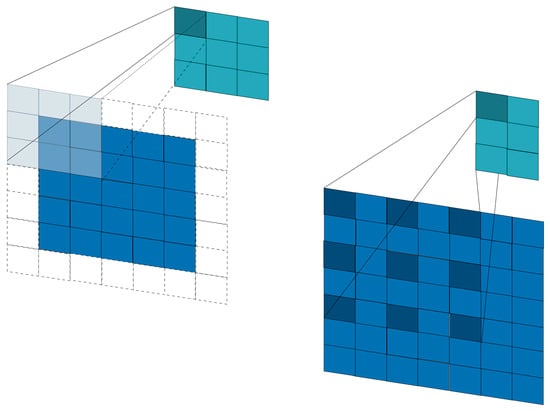
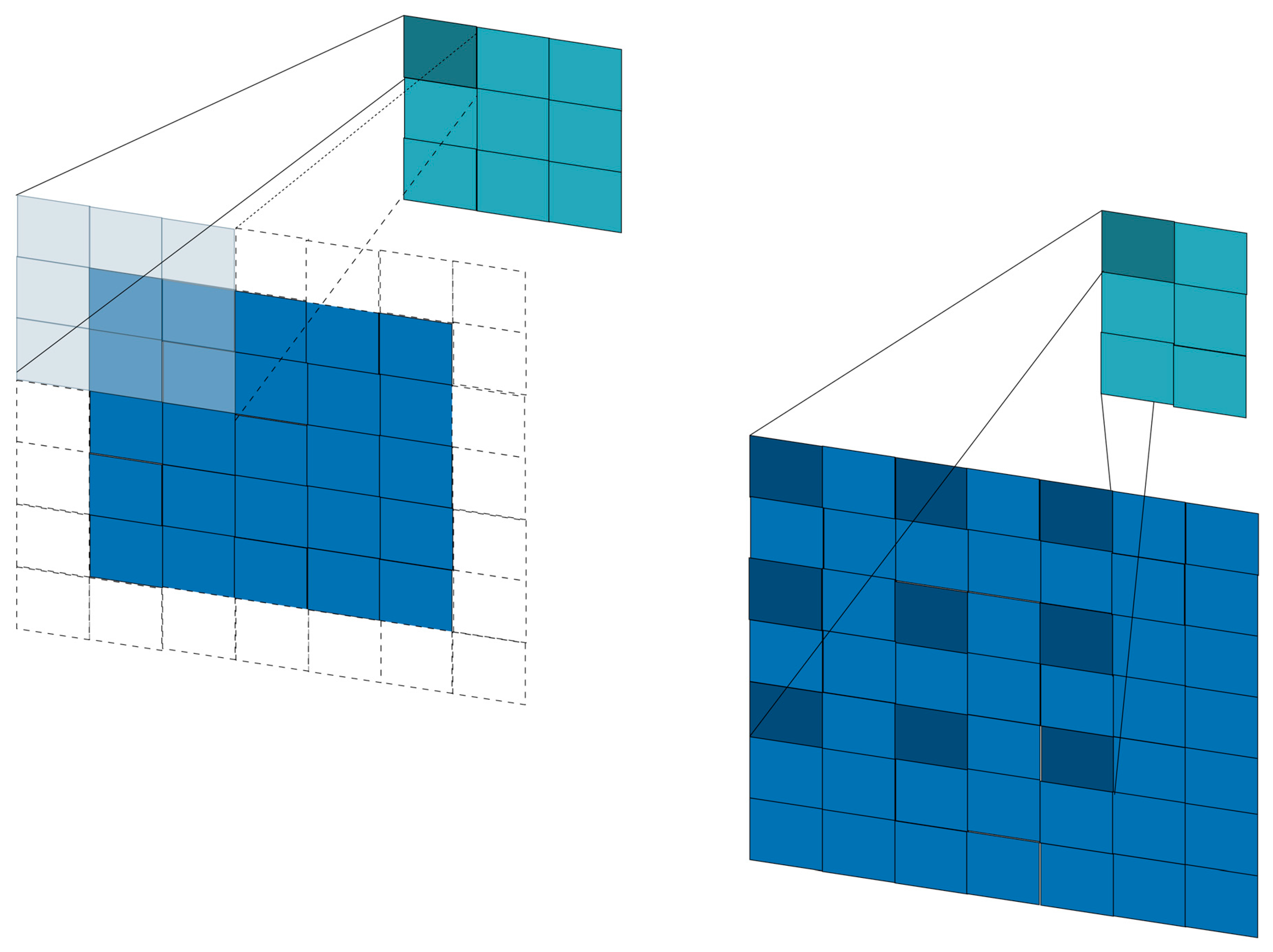
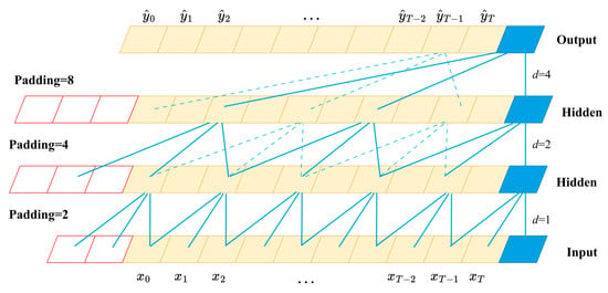
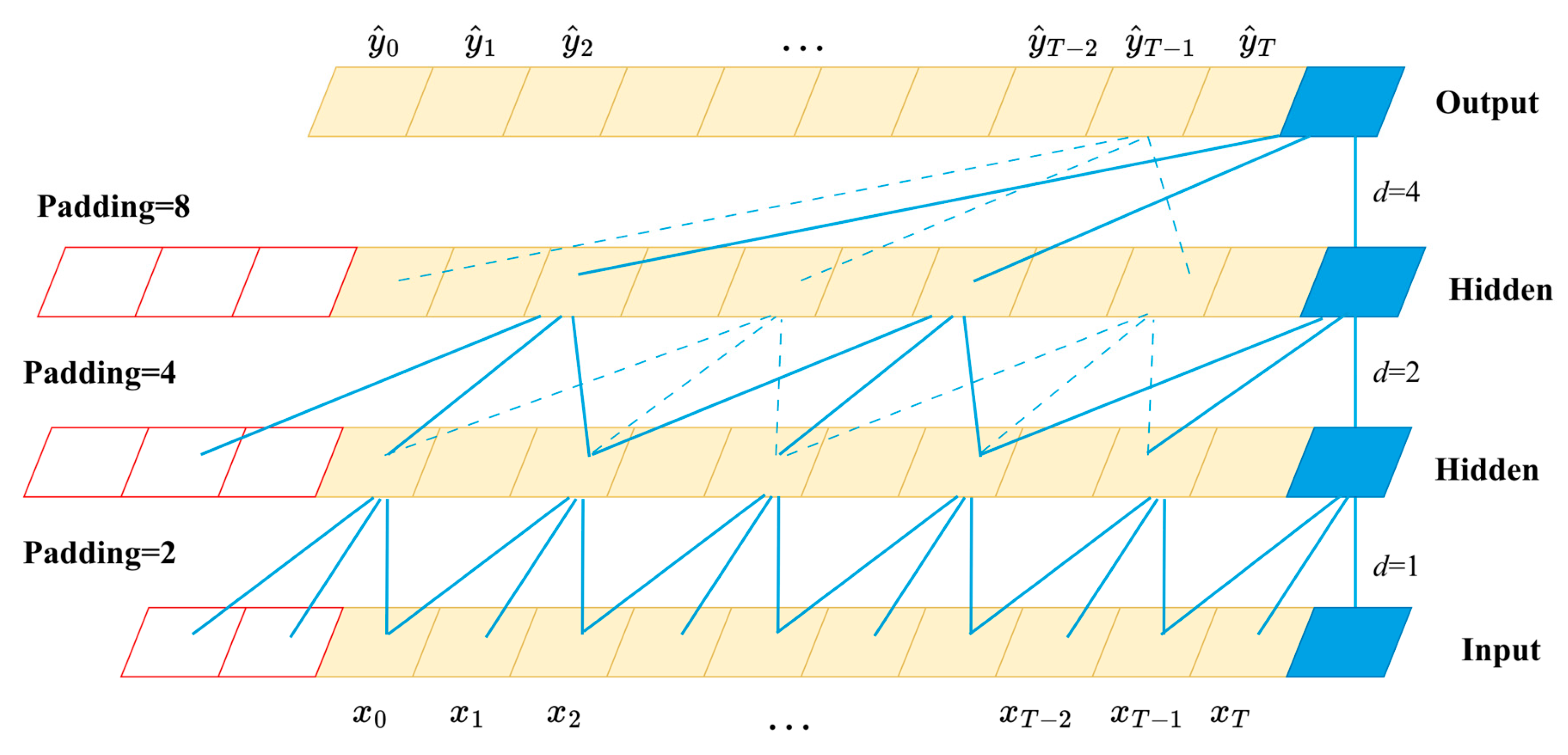
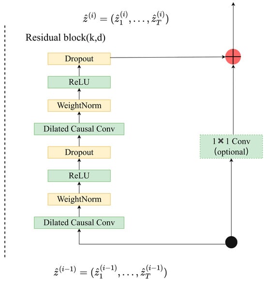
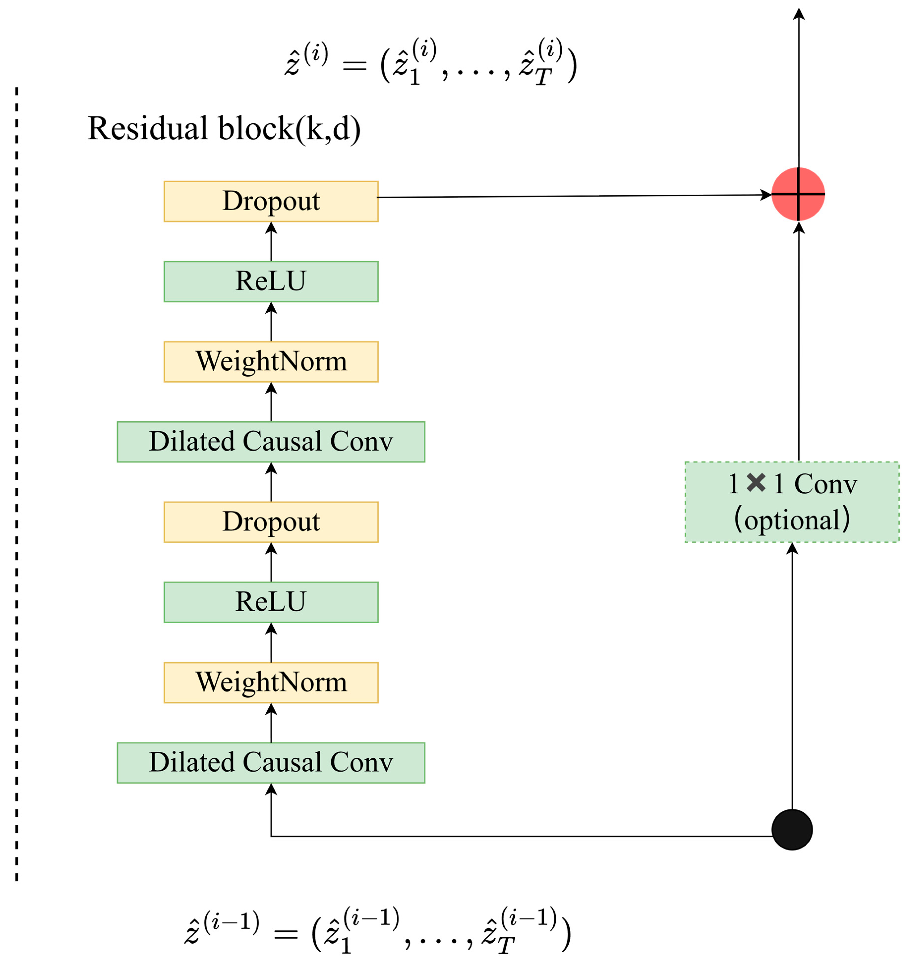
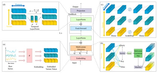
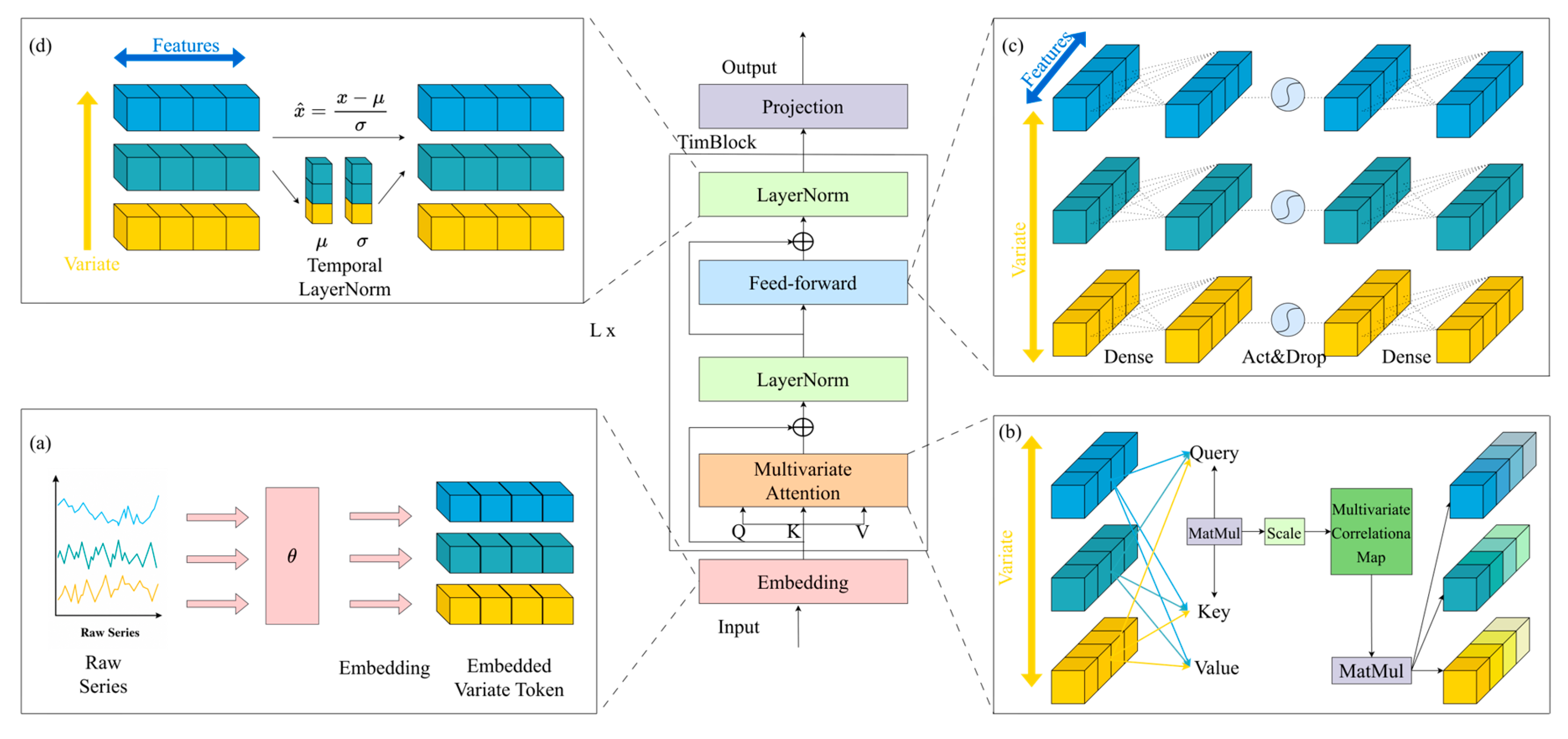
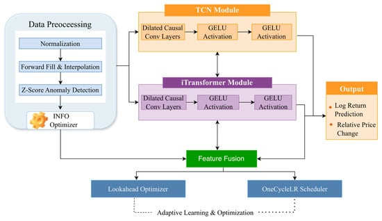
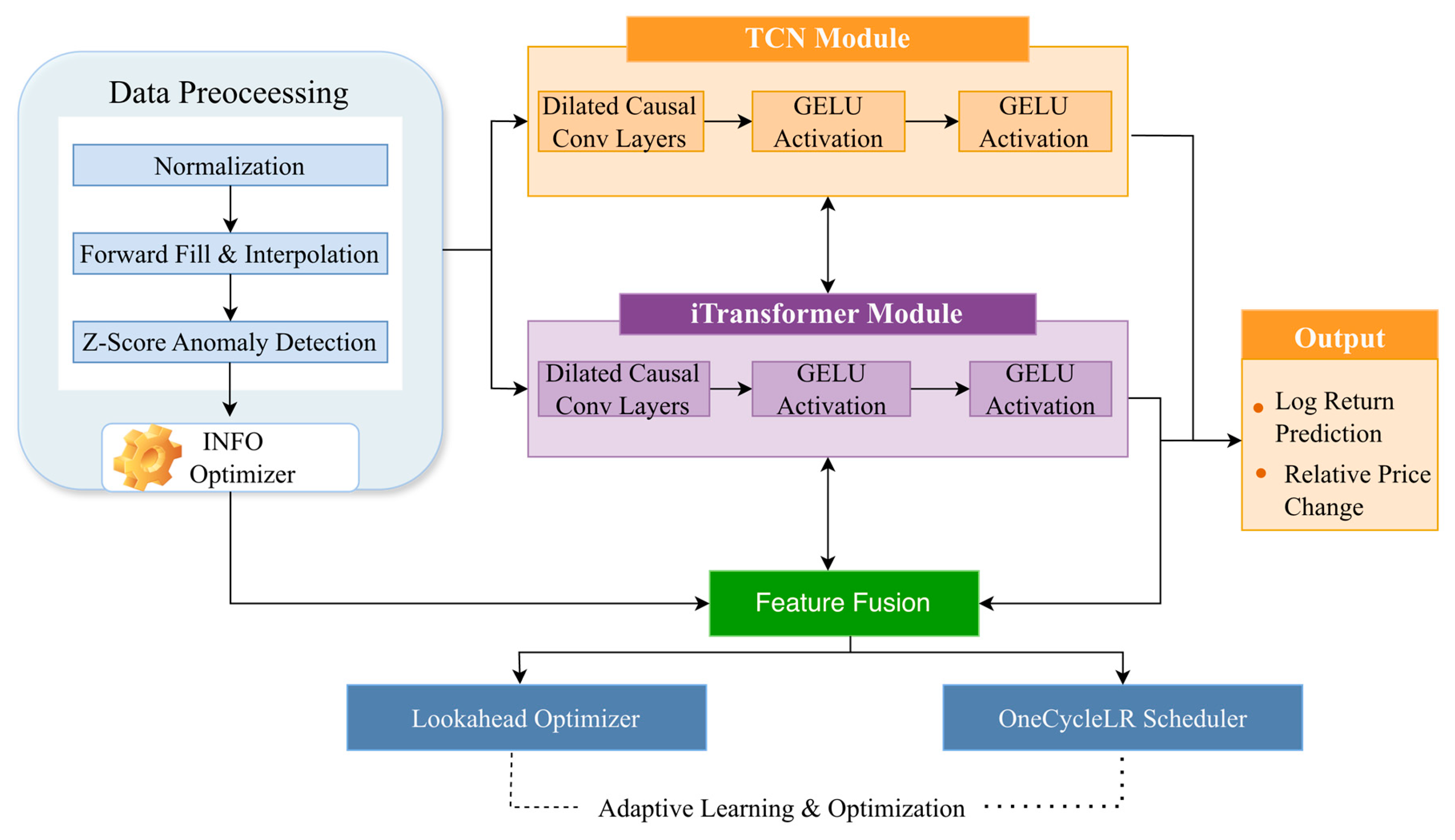
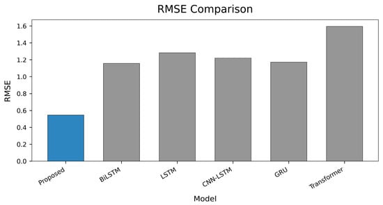
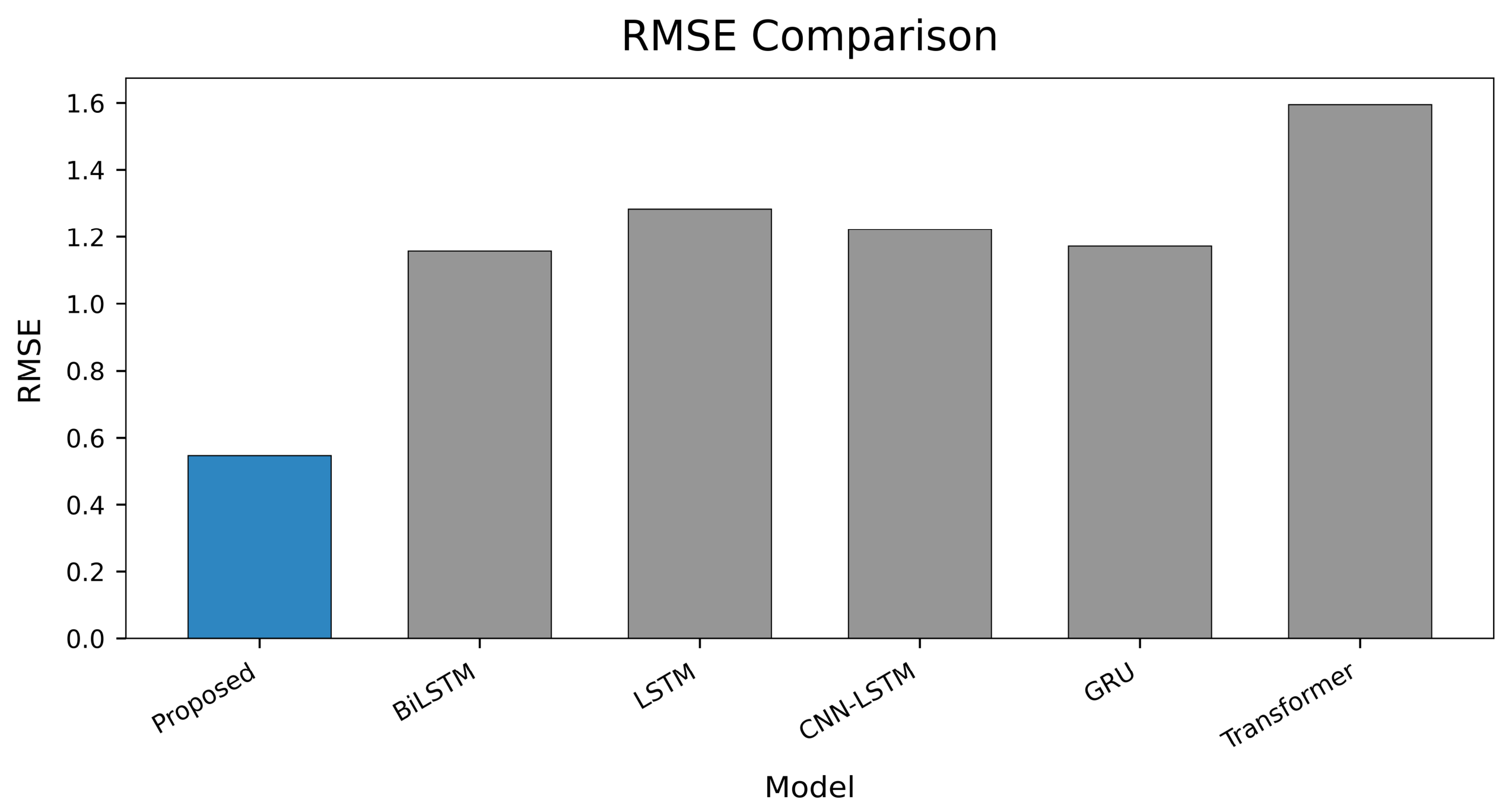
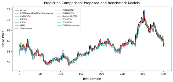
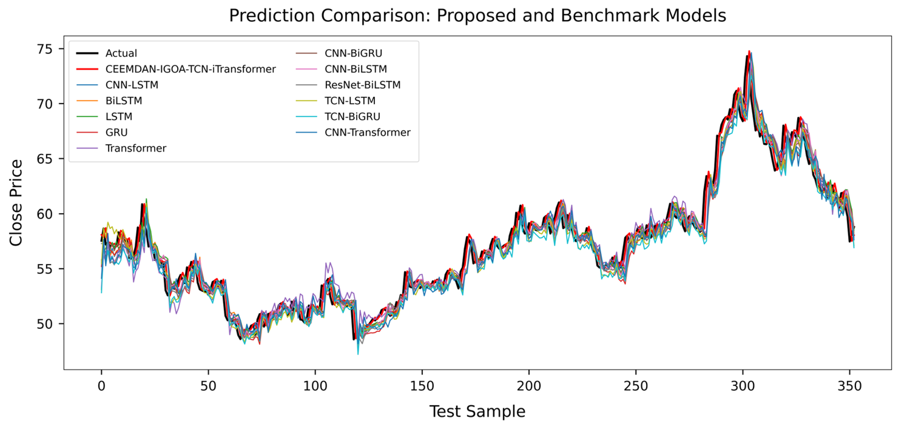
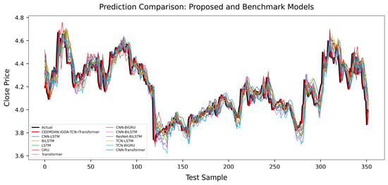
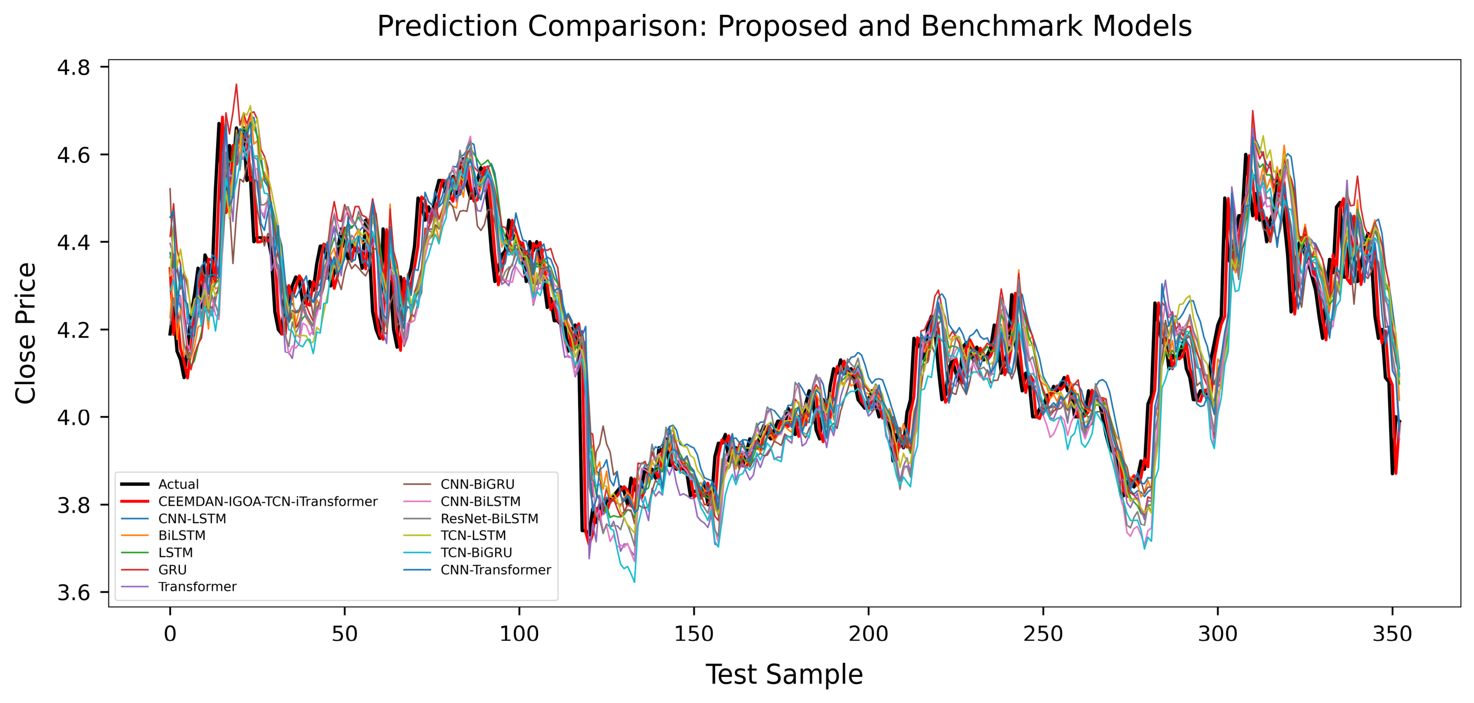
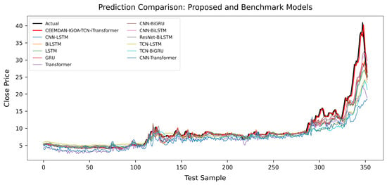
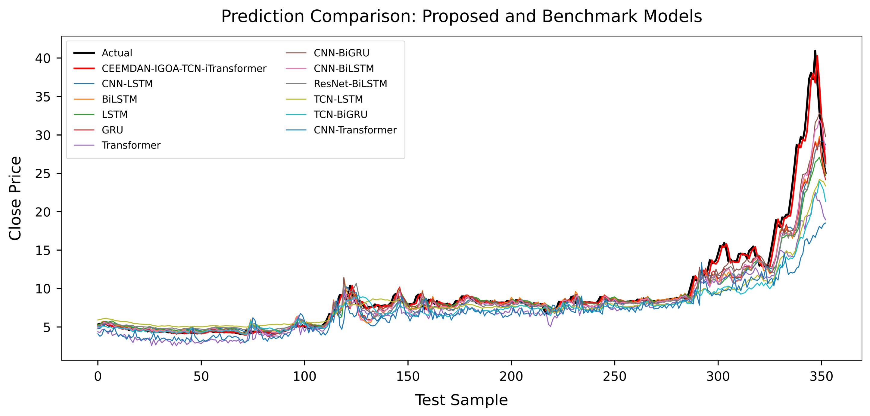
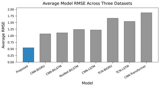
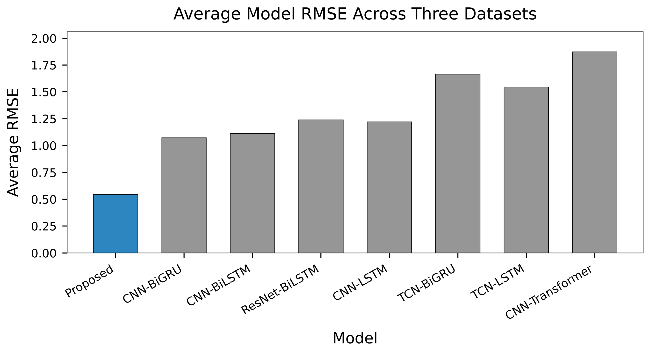
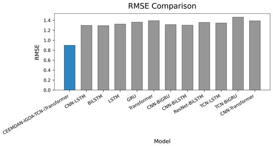
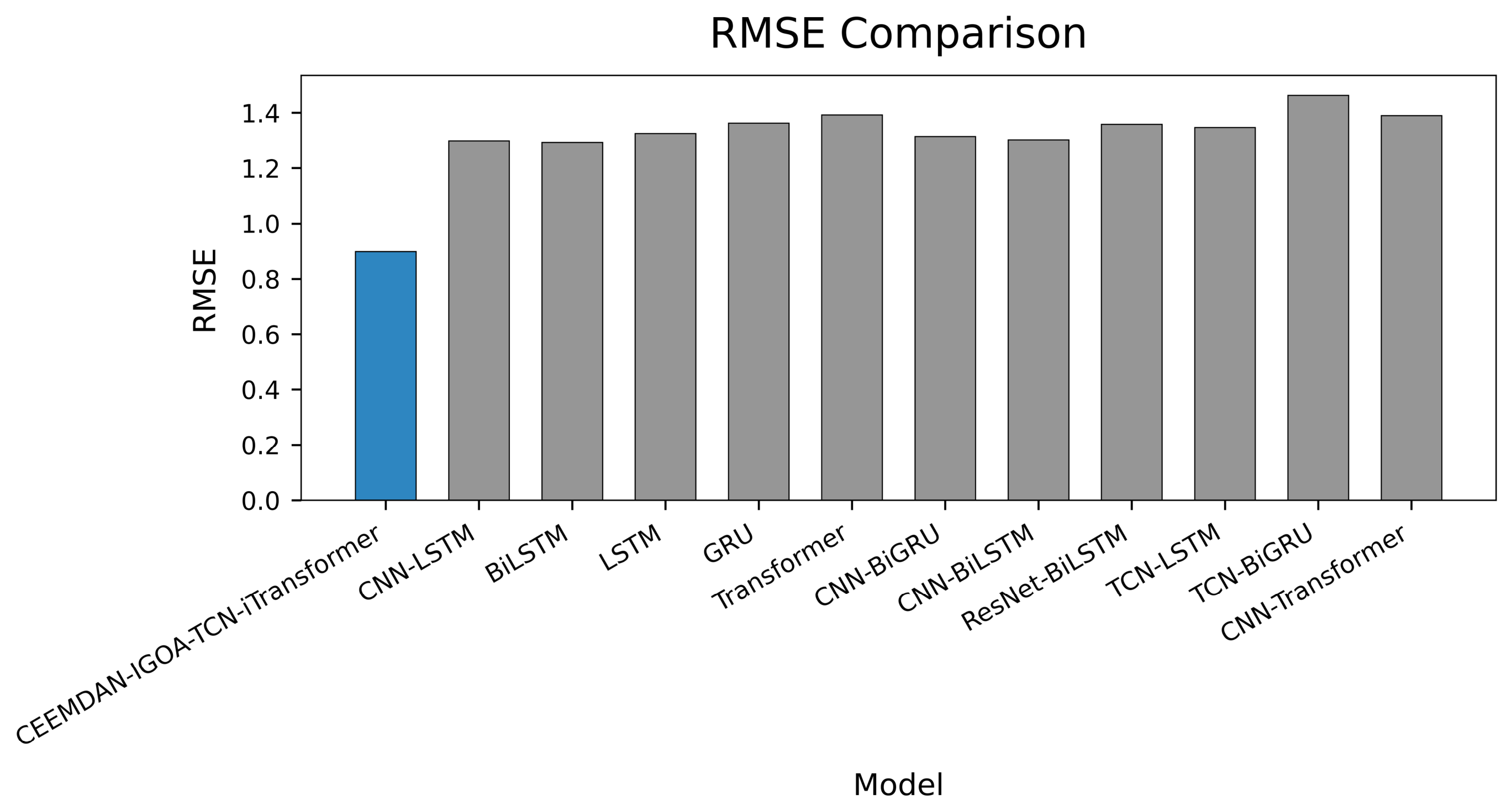
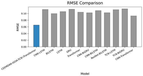
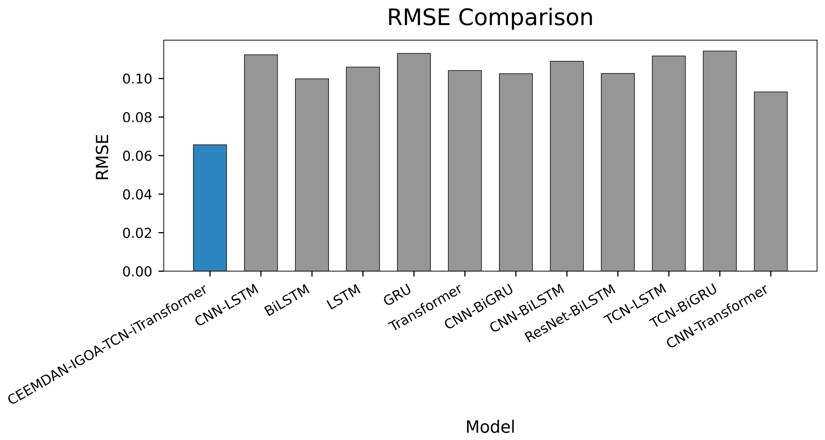
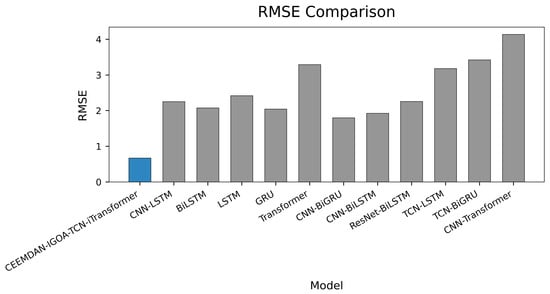
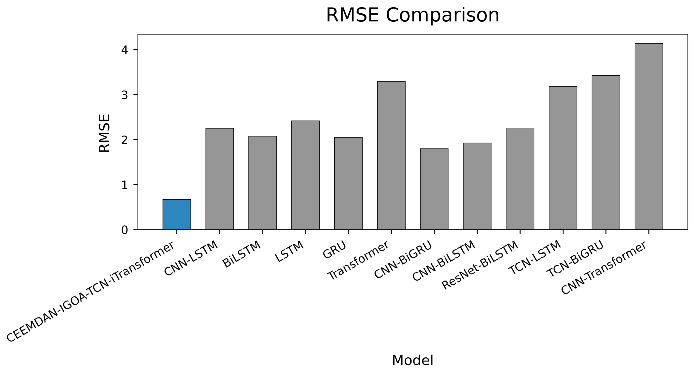
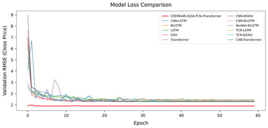
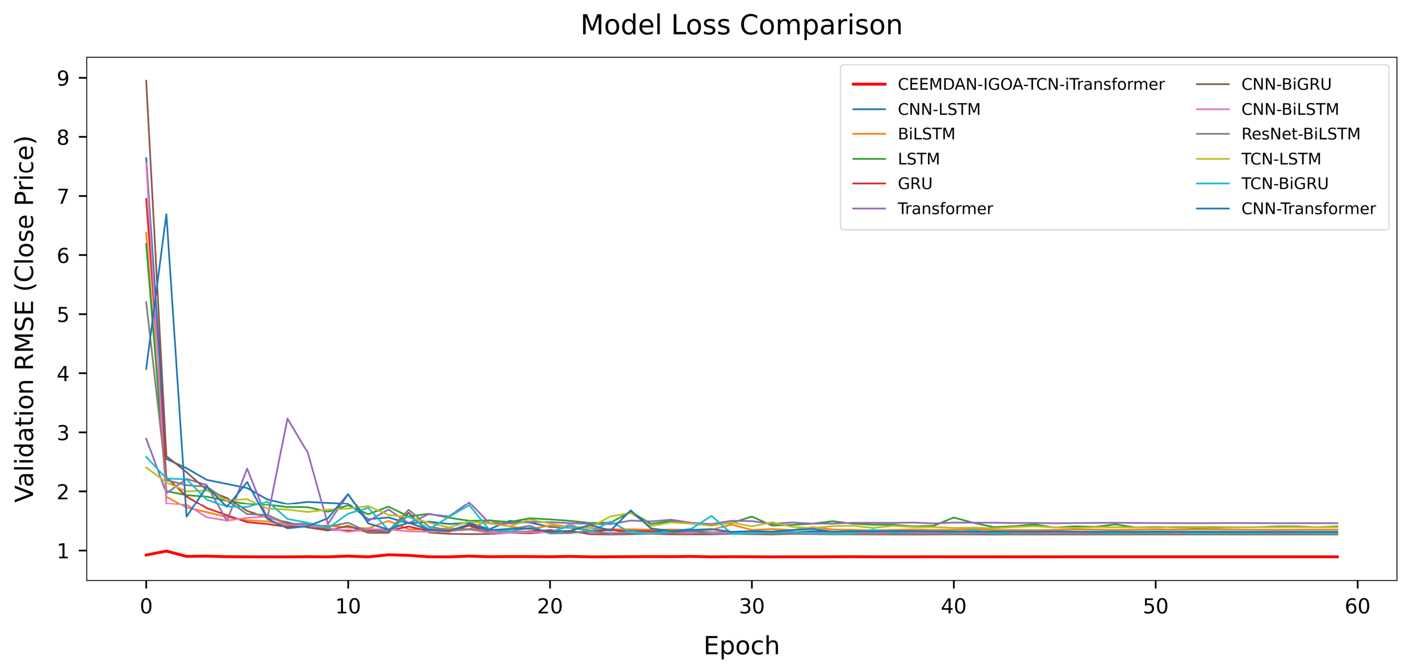
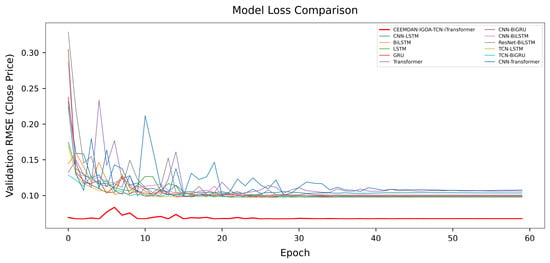
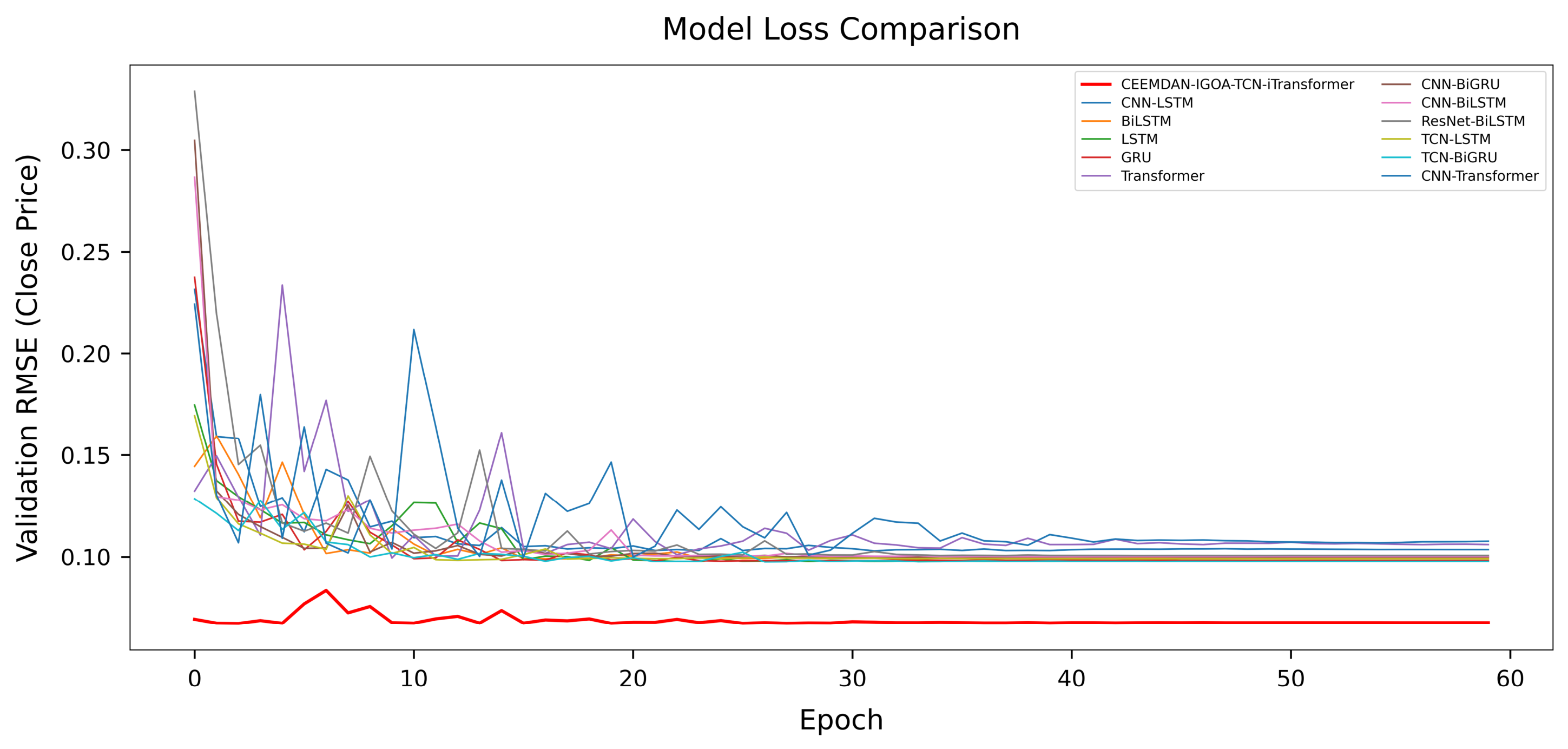
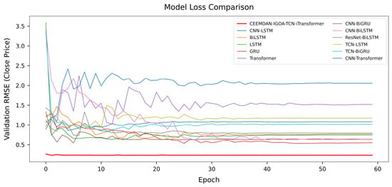
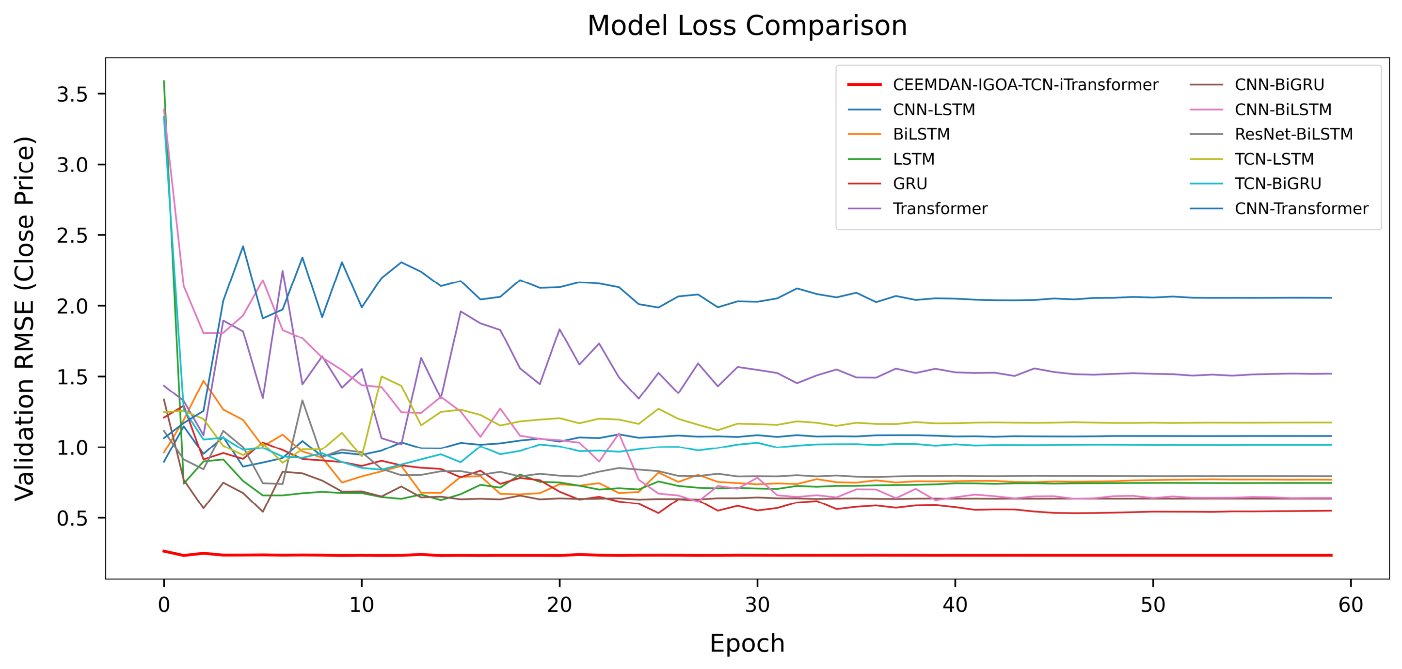
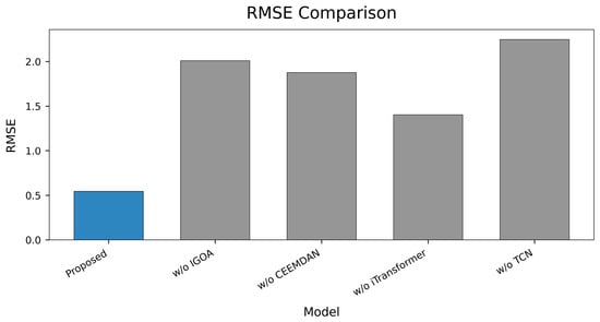
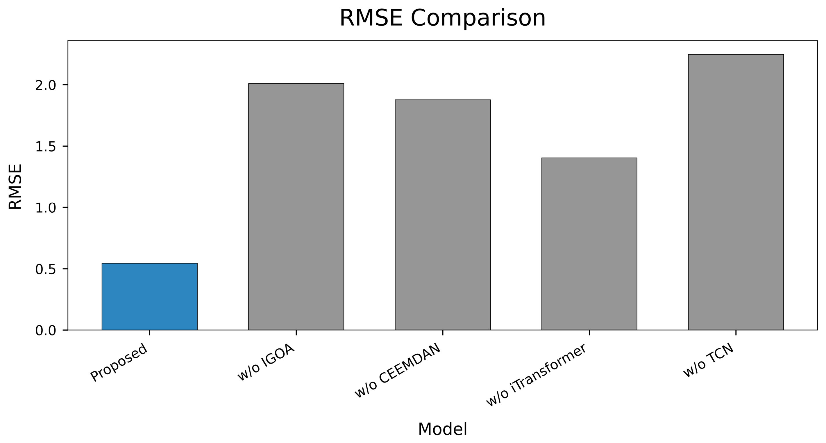
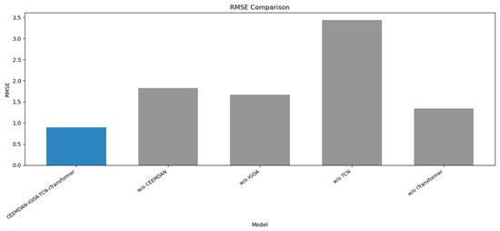
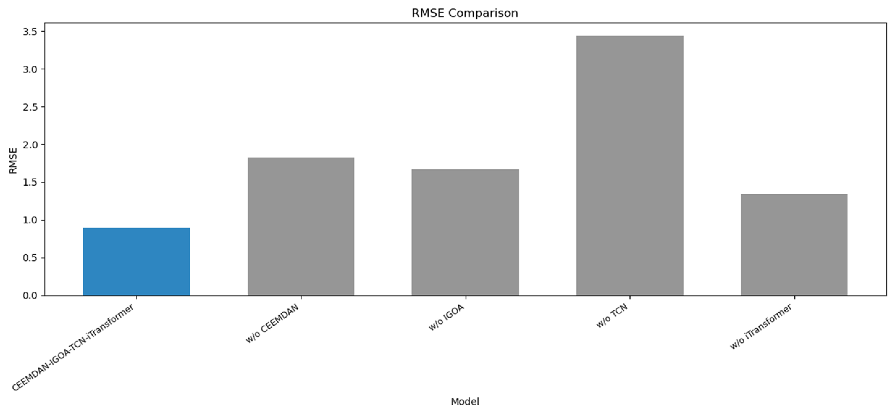
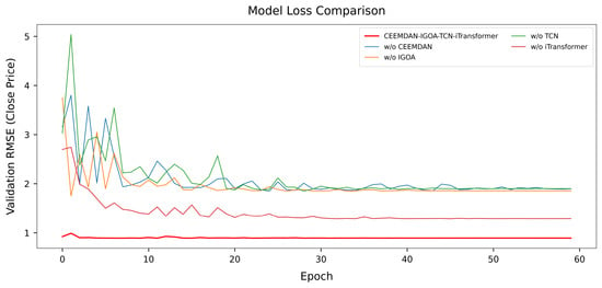
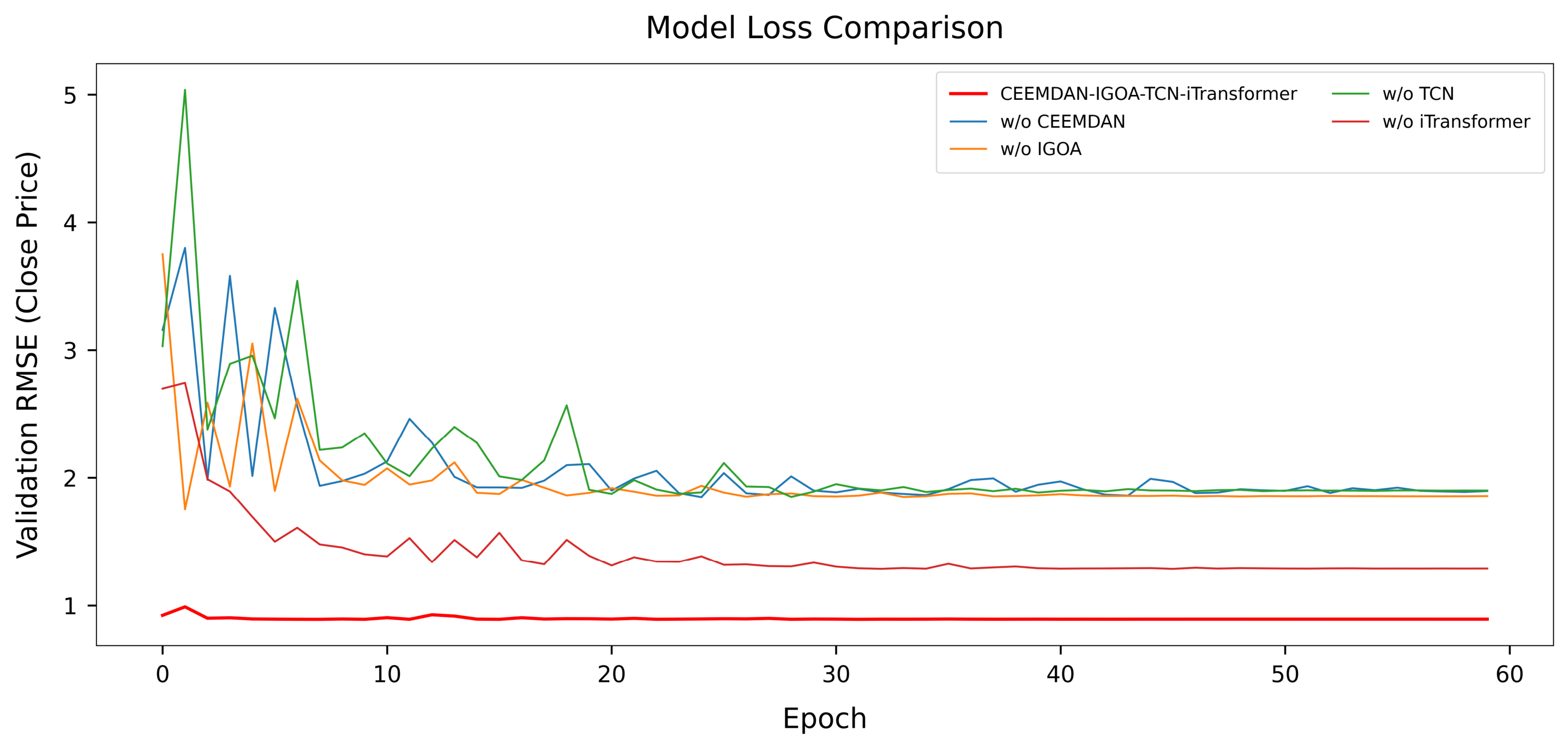
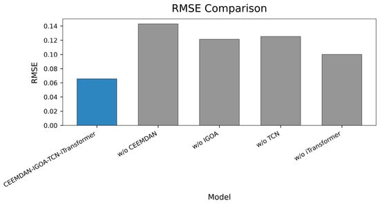
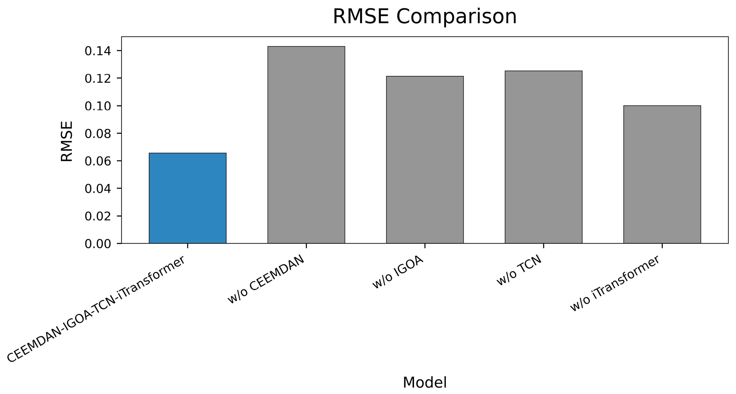
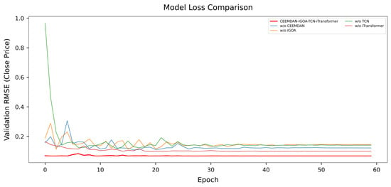
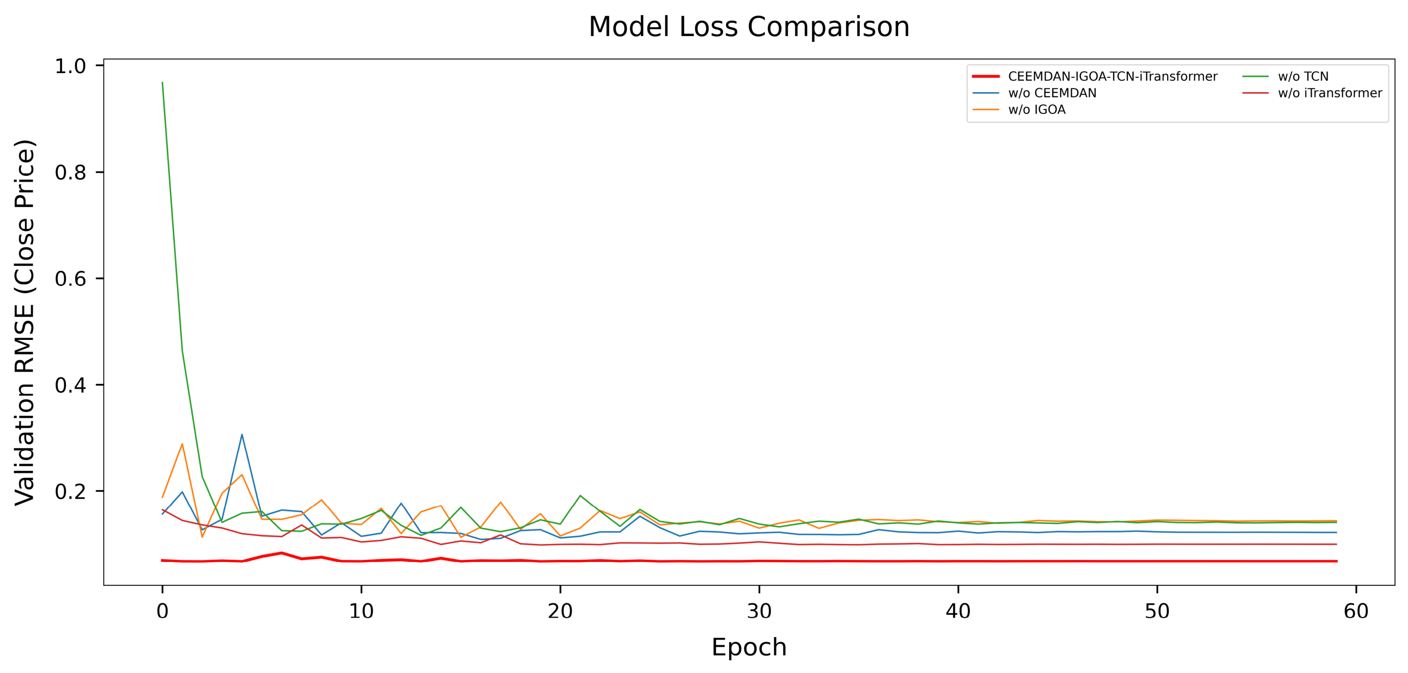
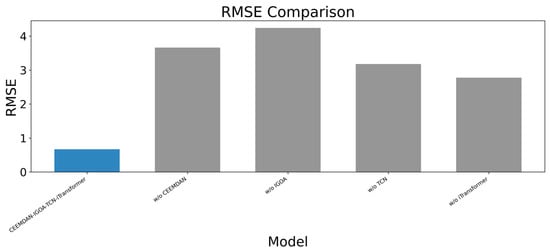
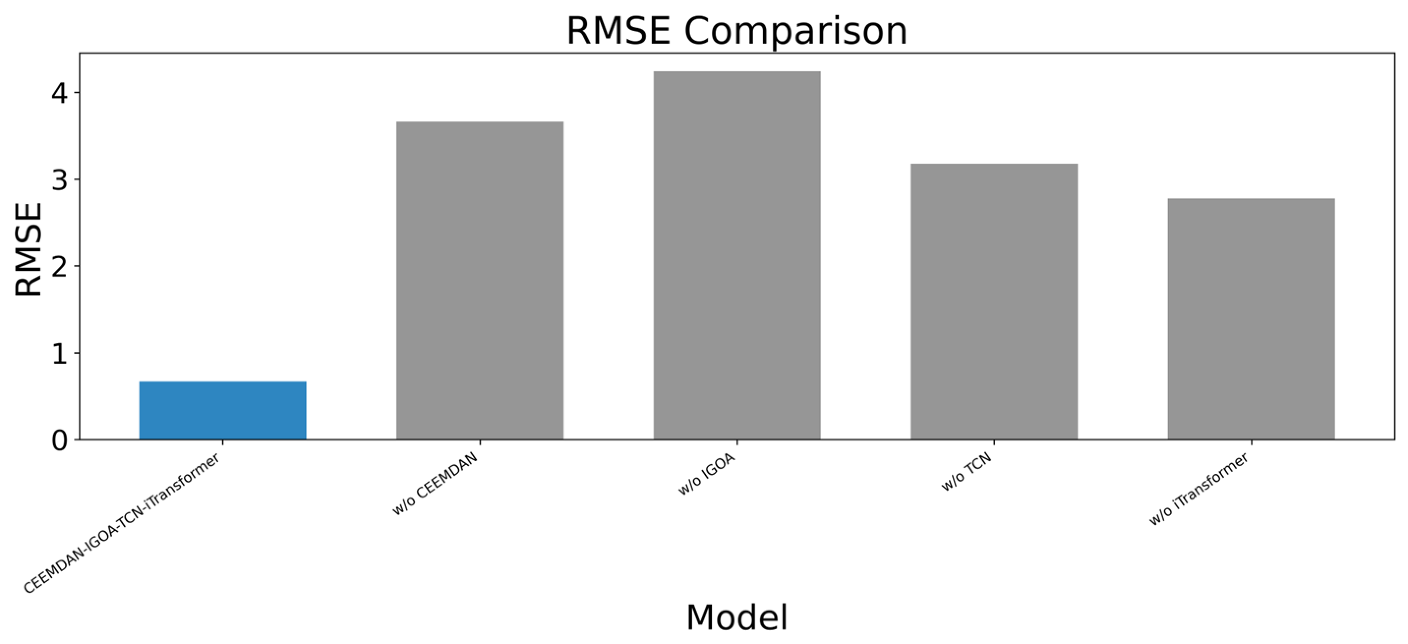
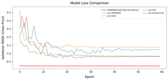
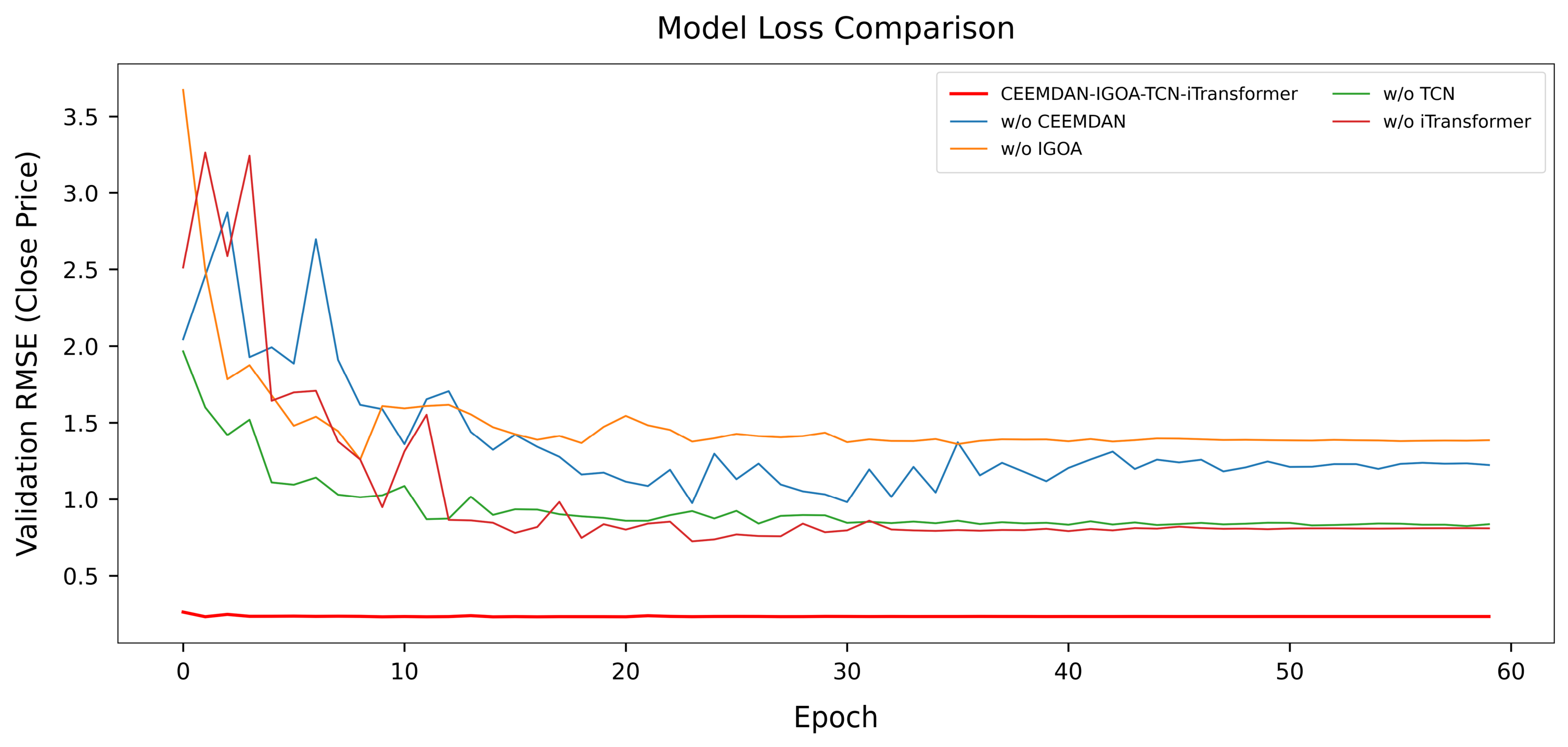
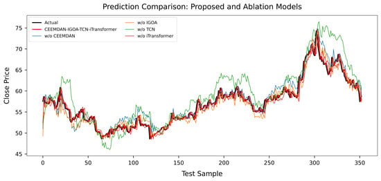
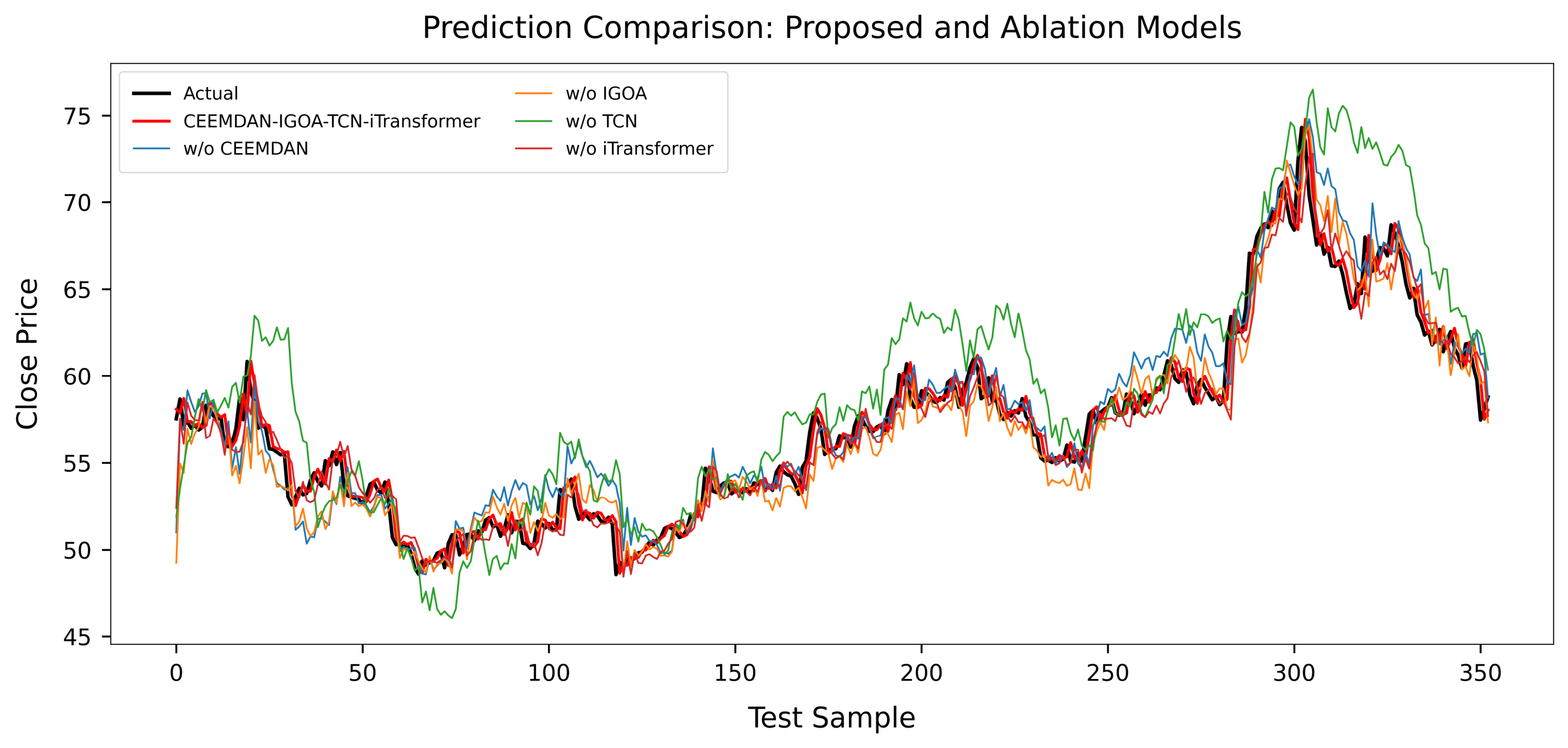
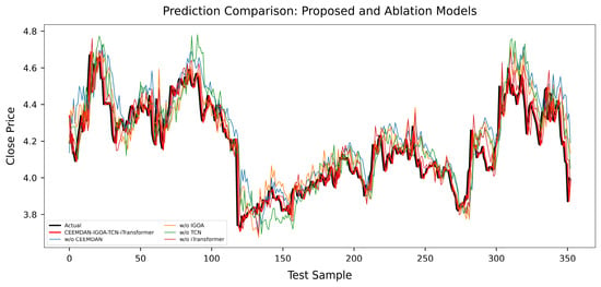
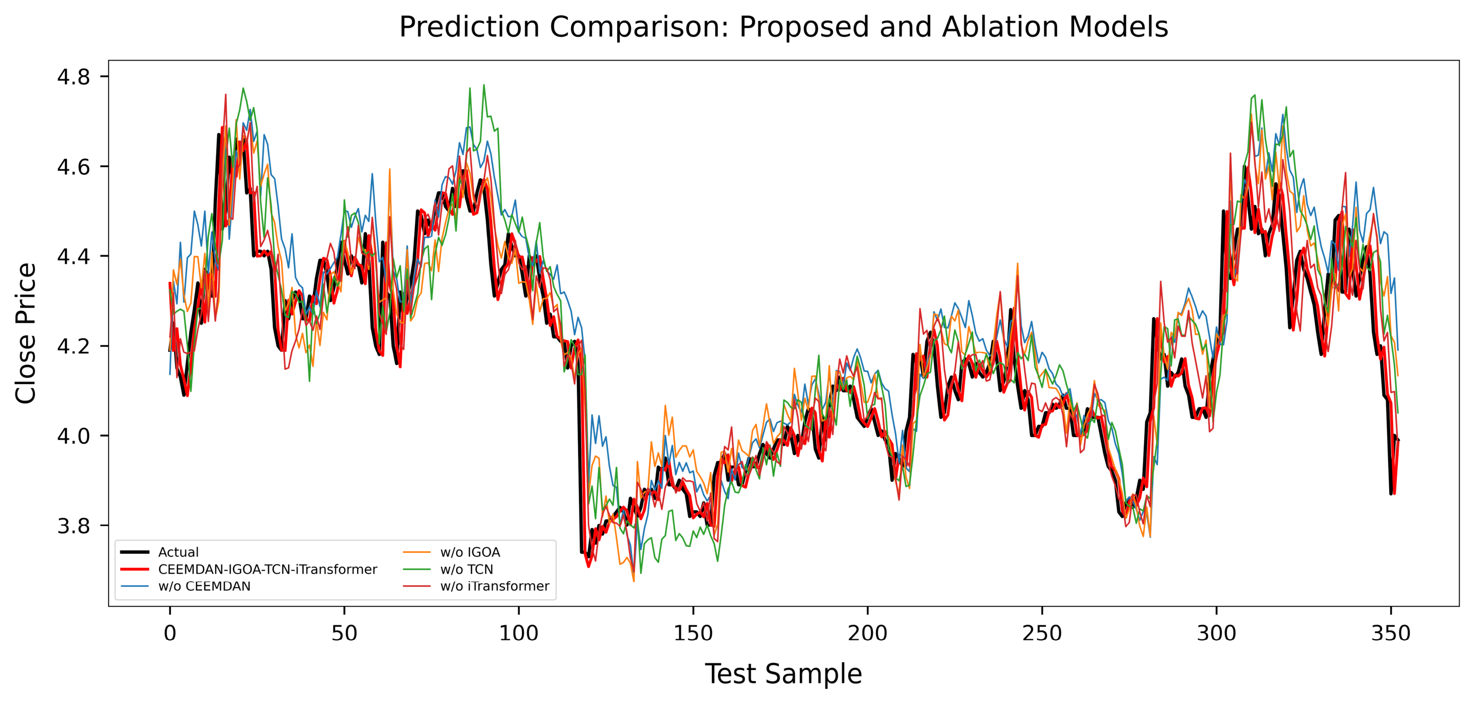
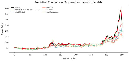
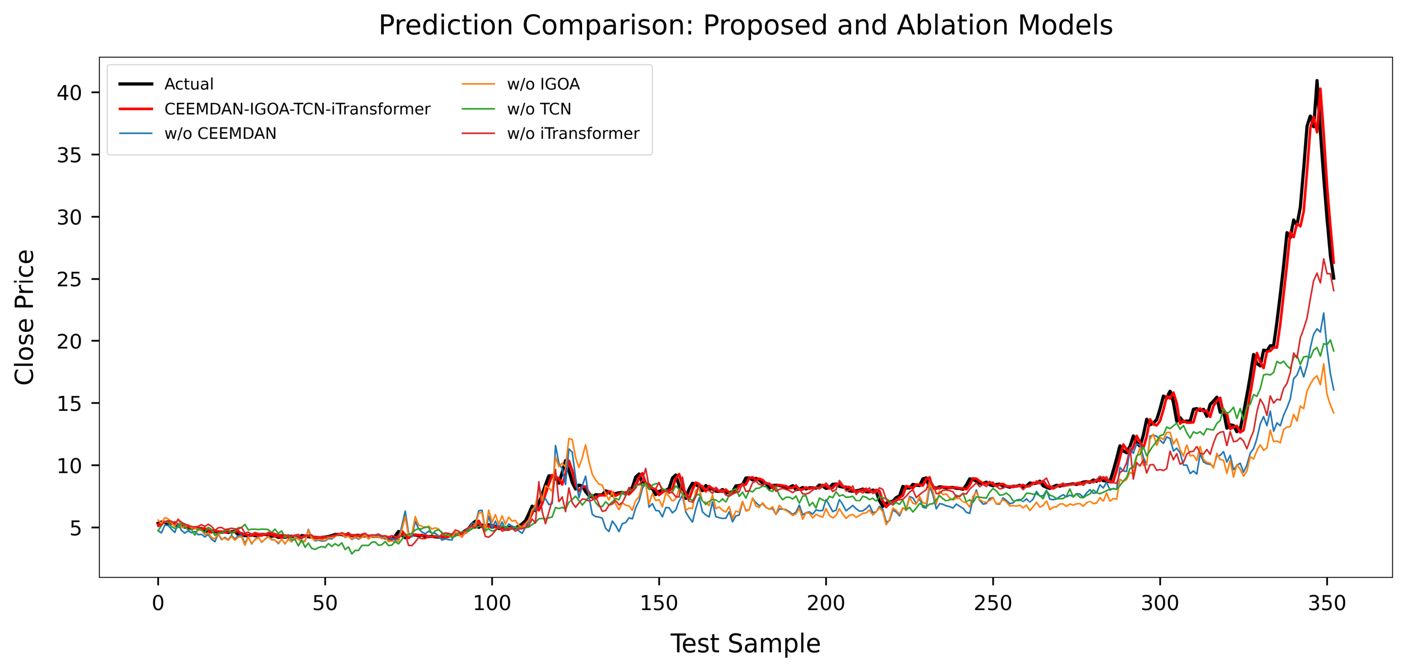
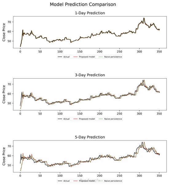
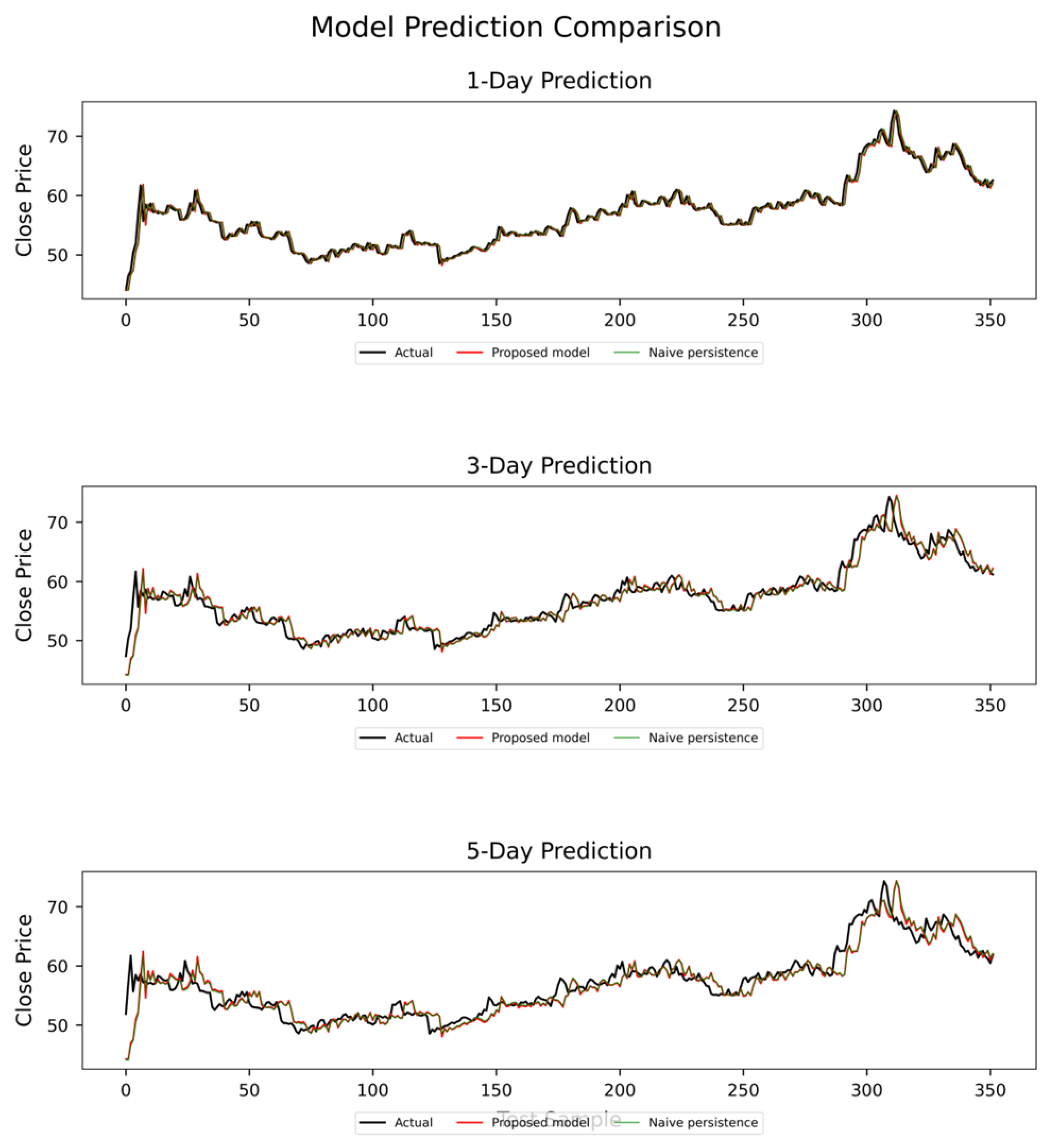
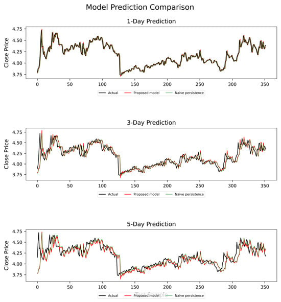
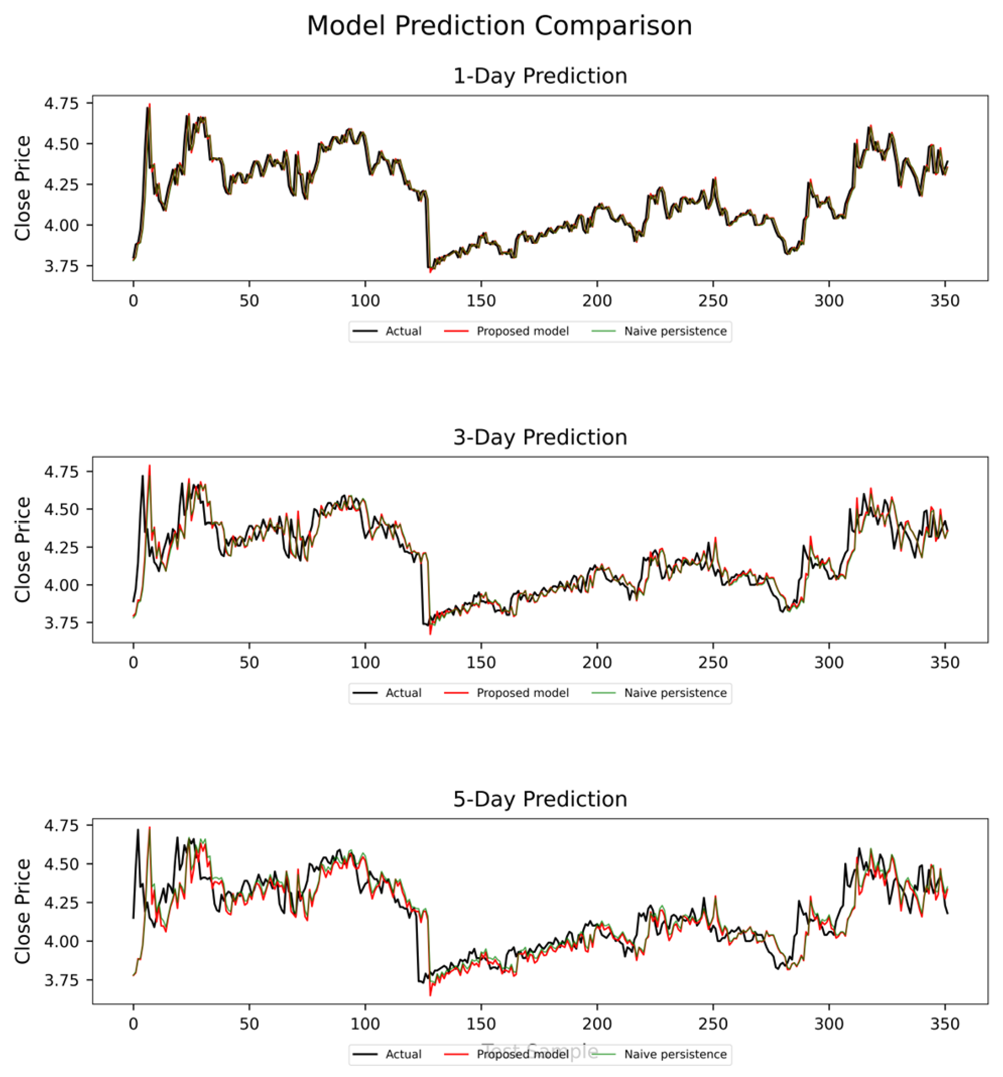
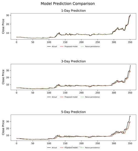
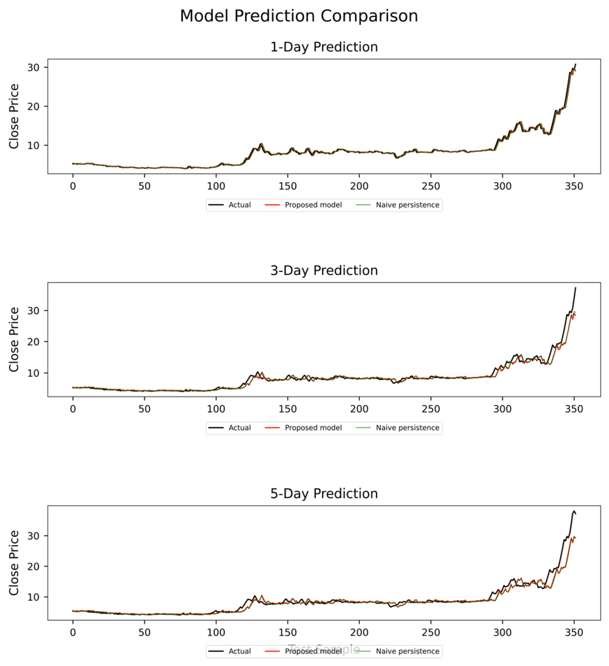

Disclaimer/Publisher’s Note: The statements, opinions and data contained in all publications are solely those of the individual author(s) and contributor(s) and not of MDPI and/or the editor(s). MDPI and/or the editor(s) disclaim responsibility for any injury to people or property resulting from any ideas, methods, instructions or products referred to in the content. |
© 2026 by the authors. Licensee MDPI, Basel, Switzerland. This article is an open access article distributed under the terms and conditions of the Creative Commons Attribution (CC BY) license.